Water-like Anomalies of Core-Softened Fluids: Dependence on the Trajectories in ($P\rho T$) Space

Abstract

In the present article we carry out a molecular dynamics study of the core-softened system and show that the existence of the water-like anomalies in this system depends on the trajectory in $P-\rho-T$ space along which the behavior of the system is studied. For example, diffusion and structural anomalies are visible along isotherms, but disappears along the isochores and isobars, while density anomaly exists along isochors. We analyze the applicability of the Rosenfeld entropy scaling relations to this system in the regions with the water-like anomalies. It is shown that the validity of the of Rosenfeld scaling relation for the diffusion coefficient also depends on the trajectory in the $P-\rho-T$ space along which the kinetic coefficients and the excess entropy are calculated.

I I. Introduction

It is well known that some liquids (for example, water, silica, silicon, carbon, and phosphorus) show an anomalous behavior in the vicinity of their freezing lines deben2003 ; bul2002 ; angel2004 ; book ; book1 ; deben2001 ; netz ; stanley1 ; ad1 ; ad2 ; ad3 ; ad4 ; ad5 ; ad6 ; ad7 ; ad8 ; errington ; errington2 . The water phase diagrams have regions where a thermal expansion coefficient is negative (density anomaly), self-diffusivity increases upon compression (diffusion anomaly), and the structural order of the system decreases with increasing pressure (structural anomaly) deben2001 ; netz . The regions where these anomalies take place form nested domains in the density-temperature deben2001 (or pressure-temperature netz ) planes: the density anomaly region is inside the diffusion anomaly domain, and both of these anomalous regions are inside a broader structurally anomalous region. It is reasonable to relate this kind of behavior to the orientational anisotropy of the potentials, however, a number of studies demonstrate waterlike anomalies in fluids that interact through spherically symmetric potentials 8 ; 9 ; 10 ; 11 ; 12 ; 13 ; 14 ; 15 ; 16 ; 17 ; 18 ; 19 ; 20 ; bar2 ; 21 ; 22 ; 23 ; 24 ; 25 ; 26 ; barb2008-1 ; barb2008 ; FFGRS2008 ; RS2002 ; RS2003 ; FRT2006 ; GFFR2009 ; fr1 ; fr2 .

As it was mentioned above, three types of anomalies are the most discussed in literature with respect to the core-softened fluids - diffusion anomaly, density anomaly and structural anomaly. Here we briefly discuss these anomalies.

If we consider a simple liquid (for, example, Lennard-Jones liquid), and trace the diffusion along an isotherm we find that the diffusion decreases under densification. This observation is intuitively clear - if density increases the free volume decreases and the particles have less freedom to move. However, some substances have a region in density - temperature plane where diffusion grows under densification. This is called anomalous diffusion region which reflects the contradiction of this behavior with the free volume picture described above. This means that diffusion anomaly involves more complex mechanisms which will be discussed below.

The second anomaly mentioned above is density anomaly. It means that density increases upon heating or that the thermal expansion coefficient becomes negative. Using the thermodynamic relation $\left(\partial P/\partial T\right)_{V}=\alpha_{P}/K_{T}$, where $\alpha_{P}$ is a thermal expansion coefficient and $K_{T}$ is the isothermal compressibility and taking into account that $K_{T}$ is always positive and finite for systems in equilibrium not at a critical point, we conclude that density anomaly corresponds to minimum of the pressure dependence on temperature along an isochor. This is the most convenient indicator of density anomaly in computer simulation.

The last anomaly we discuss here is structural anomaly. Initially this anomaly was introduced via order parameters characterizing the local order in liquid. However, later on the local order was also related to excess entropy of the liquid which is defined as the difference between the entropy and the ideal gas entropy at the same $(\rho,T)$ point: $S_{ex}=S-S_{id}$. In normal liquid excess entropy is monotonically decaying function of density along an isotherm while in anomalous liquids it demonstrates increasing in some region. This allows to define the boundaries of structural anomaly at given temperature as minimum and maximum of excess entropy.

The problem of anomalous behavior of core-softened fluids was widely discussed in literature (see, for example, the recent review fr1 ). It was shown that for some systems the anomalies take place while for others does not. In this respect the question of criteria of anomalous behavior appearance remains the central one. However, another important point is still lacking in the literature - the behavior of anomalies along different thermodynamic trajectories. Here we call as ”trajectory” a set of points belonging to some path in $(P,\rho,T)$ space. For example, the set of points belonging to the same isotherm we call as ”isothermal trajectory” or shortly isotherm.

In our previous work we showed werostr that anomalies can exist along some trajectories while along others the liquid behaves as a simple one. Taking into account this result, it is interesting to study the behavior of the quantities demonstrating anomalies along the different physically significant trajectories (isotherms, isochors, isobars and adiabats). This investigation will allow to get deeper understanding of the relations between anomalous behavior and thermodynamic parameters of the system which spread light on the connection between thermodynamic, structural and dynamic properties of liquids.

II II. System and Methods

The simplest form of core-softened potential is the so called Repulsive Step Potential which is defined as following:

$$\Phi(r)=\left\{\begin{array}[]{lll}\infty,&r\leq d\\ \varepsilon,&d<r\leq\sigma\\ 0,&r>\sigma\end{array}\right.$$ (1)

where $d$ is the diameter of the hard core, $\sigma$ is the width of the repulsive step, and $\varepsilon$ its height. In the low-temperature limit $\tilde{T}\equiv k_{B}T/\varepsilon<<1$ the system reduces to a hard-sphere systems with hard-sphere diameter $\sigma$, whilst in the limit $\tilde{T}>>1$ the system reduces to a hard-sphere model with a hard-sphere diameter $d$. For this reason, melting at high and low temperatures follows simply from the hard-sphere melting curve $P=cT/\sigma^{\prime 3}$, where $c\approx 12$ and $\sigma^{\prime}$ is the relevant hard-sphere diameter ($\sigma$ and $d$, respectively). A changeover from the low-$T$ to high-$T$ melting behavior should occur for $\tilde{T}={\mathcal{O}}(1)$. The precise form of the phase diagram depends on the ratio $s\equiv\sigma/d$. For large enough values of $s$ one should expect to observe in the resulting melting curve a maximum that should disappear as $s\rightarrow 1$. The phase behavior in the crossover region may be very complex, as shown in FFGRS2008 ; GFFR2009 .

In the present simulations we have used a smoothed version of the repulsive step potential (Eq. (1)), which has the form:

$$\Phi(r)=\left(\frac{d}{r}\right)^{n}+\frac{1}{2}\varepsilon\left(1-\tanh\left(k_{0}\left(r-\sigma_{s}\right)\right)\right)$$ (2)

where $n=14,k_{0}=10$. We have considered $\sigma_{s}=1.35$. Here and below we refer to this potential as to smooth Repulsive Shoulder System (RSS).

In the remainder of this paper we use the dimensionless quantities: $\tilde{{\bf r}}\equiv{\bf r}/d$, $\tilde{P}\equiv Pd^{3}/\varepsilon,$ $\tilde{V}\equiv V/Nd^{3}\equiv 1/\tilde{\rho}$. As we will only use these reduced variables, we omit the tildes.

In Refs. FFGRS2008 ; GFFR2009 , phase diagrams of repulsive-step models were reported for $\sigma_{s}=1.15,1.35,1.55,1.8$. To determine the phase diagram at non-zero temperature, we performed NVT MD simulations combined with free-energy calculations. For equilibration rescaling of the velocities was used, for sampling we used NVE ensemble monitoring the stability of the temperature. In all cases, periodic boundary conditions were used. The number of particles varied between 250, 500 and 864. No system-size dependence of the results was observed. The system was equilibrated for $5\times 10^{6}$ MD time steps. Data were subsequently collected during $3\times 10^{6}\delta t$ where the time step $\delta t=5\times 10^{-5}$.

In order to map out the phase diagram of the system, we computed its Helmholtz free energy using thermodynamic integration: the free energy of the liquid phase was computed via thermodynamic integration from the dilute gas limit book_fs , and the free energy of the solid phase was computed by thermodynamic integration to an Einstein crystal book_fs ; fladd . In the MC simulations of solid phases, data were collected during $5\times 10^{4}$ cycles after equilibration. To improve the statistics (and to check for internal consistency) the free energy of the solid was computed at many dozens of different state-points and fitted to multinomial function. The fitting function we used is $a_{p,q}T^{p}V^{q}$, where $T$ and $V=1/\rho$ are the temperature and specific volume and powers $p$ and $q$ are connected through $p+q\leq N$. The value N we used for the most of calculations is 5. For the low-density FCC phase N was taken equal to 4, since we had less data points. The transition points were determined using a double-tangent construction.

The region where thermodynamic anomalies are expected is situated close to the region where the system undergoes structural arrest. As a consequence, proper sampling of the phase space can be problematic. To overcome this problem we used parallel tempering book_fs . Instead of simulating a single system, we consider $n$ systems, each running in the NVT ensemble at a different temperature. Systems at high temperatures go easily over potential barriers and systems at low temperatures sample the local free energy minima. The idea of parallel tempering is to attempt Monte Carlo temperature swaps between the systems at different temperatures. If the low and high temperatures are far apart, the probability to accept such a swap move is quite low. For this reason, we use a range of ’intermediate’ temperatures. During a parallel tempering simulation, we generate equilibrium configurations for the system at all the temperatures in the simulation. In most cases, we used 8 temperatures and tried to swap them 40 times. This simulation took almost 24 hours running on 8 processors in parallel at the Joint Supercomputing Center of Russian Academy of Sciences.

Fig. 1 shows the phase diagrams that we obtain from the free-energy calculations for $\sigma_{s}=1.35$. In fact, the phase diagrams for $\sigma_{s}=1.15,1.35,1.55,1.8$ were already reported in Refs. FFGRS2008 ; GFFR2009 . We show these phase diagrams here too because they provide the “landscape” in which possible “water” anomalies should be positioned.

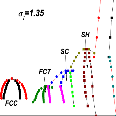
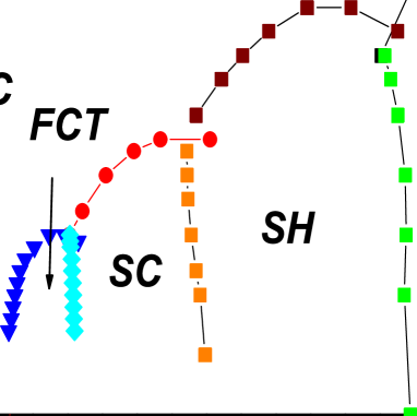
Figure 1: (Color online). Phase diagram of the system of particles interacting through the potential (2) with $\sigma_{s}=1.35$ in $\rho-T$ and $P-T$ planes.

Fig. 1(a) shows the phase diagram of the system with $\sigma_{s}=1.35$ in the $\rho-T$ plane. There is a clear maximum in the melting curve at low densities. The phase diagram consists of two isostructural FCC domains corresponding to close packing of the small and large spheres separated by a sequence of structural phase transitions. This phase diagram was discussed in detail in our previous publication FFGRS2008 ; GFFR2009 . It is important to note that there is a region of the phase diagram where we have not found any stable crystal phase. The results of Ref.  FFGRS2008 suggest that a glass transition occurs in this region with $T_{g}=0.079$ at $\rho=0.53$. The apparent glass-transition temperature is above the melting point of the low-density FCC and FCT phases. If, indeed, no other crystalline phases are stable in this region, the “glassy” phase that we observe would be thermodynamically stable. This is rather unusual for one-component liquids. In simulations, glassy behavior is usually observed in metastable mixtures, where crystal nucleation is kinetically suppressed. One could argue that, in the glassy region, the present system behaves like a “quasi-binary” mixture of spheres with diameters $d$ and $\sigma_{s}$ and that the freezing-point depression is analogous to that expected in a binary system with a eutectic point: there are some values of the diameter ratio such that crystalline structures are strongly unfavorable and the glass phase could then be stable even at very low temperatures. The glassy behavior in the reentrant liquid disappears at higher temperatures.

III III. Results and discussion

III.1 Diffusion anomaly

The diffusion anomaly of the RSS was discussed in several our previous articles. In the Refs. FFGRS2008 and GFFR2009 we showed that the diffusion anomaly takes place at the shoulder width $\sigma_{1}=1.35$ while in the work weros the breakdown of the Rosenfeld scaling for this system was demonstrated. Further discussion of the Rosenfeld scaling was reported in the work werostr . The main idea of this paper is that the anomalous diffusion behavior present along low-temperature isotherms while along isochors diffusion coefficient is monotonous. As a result, Rosenfeld scaling is valid along isochors and high-temperature isotherms, however, it breaks down for the isotherms with anomalies. It means that appearance or not of anomalies at some trajectory can cause physically different behavior of the system. As a result, following different trajectories, we can or can not observe some effects. It is of particular importance since experimental works deal mostly with isobars and isotherms while theoretical studies - with isochors and isotherms. Taking this into account, one can expect that some of the effects observed along isobars are not visible along isotherms and isochors which makes us confused while comparing experimental results with theoretical predictions. Here we extend the study of anomalies to four different physically meaningful trajectories: isotherms, isochors, isobars and adiabats.

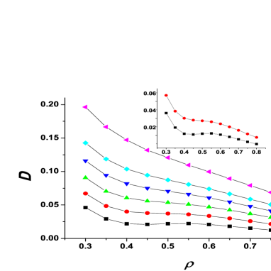
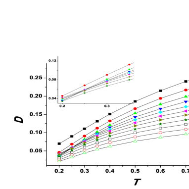
Figure 2: (Color online). Diffusion coefficient of the RSS system along (a) isotherms and (b) isochors. The insets show (a) the low temperature isotherms and (b) low temperature region of some isochors.

Fig. 2(a) shows the diffusion coefficient of RSS system along a set of isotherms for $\sigma_{1}=1.35$. One can see that the diffusion coefficient demonstrates anomalous behavior for the temperatures below $T=0.25$. However, if we look at the Fig. 2(b) where the same diffusion coefficient data are arranged along isochors we do not observe anomalies - the diffusion is a monotonous function of temperature along isochors. However, some of the isochors cross. One can see from the inset that the cross of the isochors corresponds to the densities between $\rho=0.4$ and $\rho=0.6$. Comparing it to the isotherms we see that this is the region of anomalous diffusion. It means that even if we do not see nonmonotonous behavior of diffusion along isochors we can identify the presence of anomaly from crossing of the isochors. However, this method seems to be technically more difficult since we need to measure many points belonging to different isochors rather then one isotherm.

Isothermal and isochoric behavior of diffusion in anomalous region have already been discussed in our previous publication werostr and we give these plots here for the sake of completeness. Fig. 3(a) shows the diffusion coefficient along a set of isobars as a function of density. The diffusion coefficient is again monotonous. The slope of the curves is always negative. However, as it can be seen from the inset, the slope approaches infinity at low diffusions at pressures $P=2.0$ and $P=2.5$. This corresponds to densities $0.45-0.55$ inside the anomalous region. One can imagine that if we lower the temperatures along these isobars we can observe change of the slope to positive one, however, we do not have data for these temperatures.

Fig. 3(b) shows the diffusion coefficient along isobars as a function of temperature. The situation is analogous to the case of isochors: the curves are monotonous, however, they intersect at low temperatures, corresponding to anomalous region (see the inset in Fig. 3(b)). It means that if we have the diffusion coefficient along isobars we can identify the presence of anomalies by monitoring the intersections of the curves. However, by the reasons discussed above this method is not practically convenient.

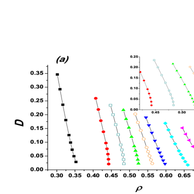
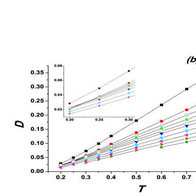
Figure 3: (Color online). Diffusion coefficient of the RSS system along isobars as a function of (a) density and (b) temperature. The insets show anomalous regions in the corresponding coordinates.

The last physically meaningful trajectory considered in the present work is the adiabat. This trajectory is defined as constant entropy curve. The entropy is calculated as following. We compute excess free energy by integrating the equation of states: $\frac{F_{ex}}{Nk_{B}T}=\frac{F-F_{id}}{Nk_{B}T}=\frac{1}{k_{B}T}\int_{0}^{\rho}\frac{P(\rho^{\prime})-\rho^{\prime}k_{B}T}{\rho^{\prime 2}}d\rho^{\prime}$. The excess entropy can be computed via $S_{ex}=\frac{U-F_{ex}}{Nk_{B}T}$. The total entropy is $S=S_{ex}+S_{id}$, where the ideal gas entropy is $\frac{S_{id}}{Nk_{B}}=\frac{3}{2}\ln(T)-\ln(\rho)+\ln(\frac{(2\pi mk_{B})^{3/2}e^{5/2}}{h^{3}})$. The last term in this expression is constant and is not accounted in our calculations.

The behavior of entropy itself will be discussed below. Here we give the diffusion coefficients along the adiabats (Fig. 4 (a)-(c)).

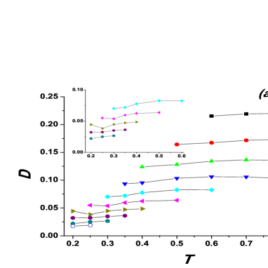
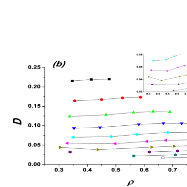
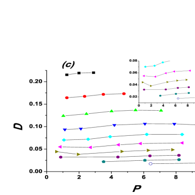
Figure 4: (Color online). Diffusion coefficient of the RSS system along adiabats as a function of (a) temperature, (b) density, and (c) pressure. The insets show anomalous regions in the corresponding coordinates.

One can see from the Fig. 4 (a)-(c) that the anomaly takes place along adiabats in all possible coordinates (look, for example, $S=-4.0$ adiabat). It means that in case of adiabatic trajectory one can identify the anomalous region monitoring any of three thermodynamic variables ($P,\rho,T$). However, this trajectory is rather difficult to realize in simulation or experiment.

III.2 Density Anomaly

As we mentioned above density anomaly corresponds to appearance of a minima on isochors of the system. The isochors are shown in the Fig. 5(a). It is evident from the figure that some of the isochors do demonstrate minima. The location of the minimum in the $\rho-T$ plane is shown in Fig. 5(b). One can see from this figure that the region of the density anomaly is located inside the region of the diffusion anomaly which is consistent with the general picture corresponding to water.

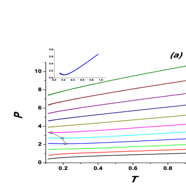
Figure 5: (Color online). (a) A set of isochors of RSS. The stars show the location of minimum. The inset enlarges the $\rho=0.45$ isochor. (b) The location of the minima on isochors in $\rho-T$ plane.

If we turn to the shape of the isobars themselves, that is the dependence of temperature on density at fixed pressure we do not find any traces of anomalies there (Fig.  6). Like in the case of diffusion, the curves have negative slope which approaches zero at low temperatures and densities corresponding to anomalous regime. However, the curve remains monotonous which means that there is no sign of density anomaly along isobars.

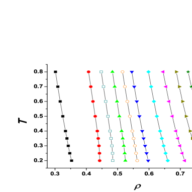
Figure 6: (Color online). A set of isobars of RSS.

Figs.  7(a) and (b) show adiabats of the RSS in $\rho-T$ and $P-T$ coordinates. Interestingly, the curves are again monotonic, but the slope of the curves at low and high densities (pressures) is very different. At the same time the middle density (pressure) curves demonstrate a continues change from the high slope (low-density regime) to low slope (high-density) regime. It allows to conclude that even if adiabats show monotonous behavior one can easily identify the location of anomalous region by the slope change of the curves.

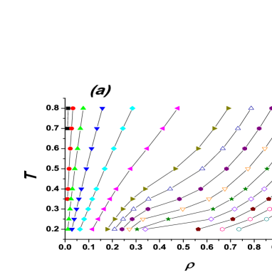
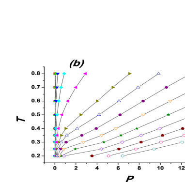
Figure 7: (Color online). Adiabats of the RSS in (a) density - temperature and (b) pressure - temperature coordinates.

III.3 Structural Anomaly

Structural anomaly region can be bounded by using the local order parameters or by excess entropy minimum and maximum. Here we apply the definition via excess entropy.

The behavior of excess entropy is qualitatively analogous to the behavior of diffusion coefficient. Because of this we briefly describe it here noting that most of the conclusions about diffusion coefficient along different trajectories can be applied to excess entropy as well.

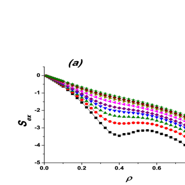
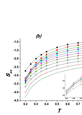
Figure 8: (Color online). Excess entropy of RSS fluid along (a) isotherms and (b) isochors.

Figs. 8(a) and (b) show the excess entropy along isotherms and isochors. Like for the diffusion coefficient, excess entropy demonstrates anomalous grows in some density range at low temperatures. At the same time excess entropy is monotonous along isochors. However, the curves for different isochors cross which indicates the presence of anomaly.

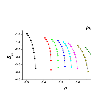
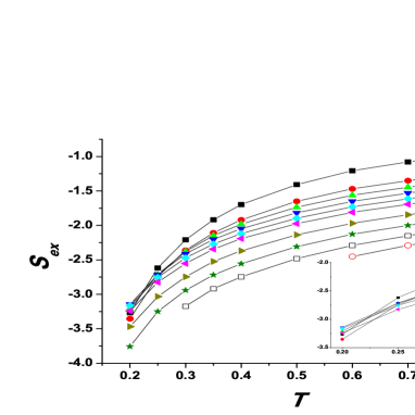
Figure 9: (Color online). Excess entropy of RSS fluid along isobars as a function of (a) density and (b) temperature. The inset in (b) shows the cross of the curves at low temperatures.

The excess entropy along isobars is monotonically decreasing function of density and monotonically increasing function of temperature. However, the curves cross at low temperatures indicating the presence of anomalies as it was discussed for the case of diffusion.

It is important to note that the range of densities of structural anomalies is wider then the one of diffusion anomaly which is consistent with the literature data for core-softened systems.

To summarize this section, we emphasize that the anomalous behavior can be seen only along some particular trajectories in $(P,\rho,T)$ space. For example, diffusion and structural anomalies are visible along isotherms while density anomaly - along isochors. Other meaningful trajectories (isobars and adiabats) can identify the presence of anomalies via crossing of the curves, but they do not allow easily identify the boundaries of the anomalous region.

IV IV. Rosenfeld scaling

In 1977 Rosenfeld proposed a connection between thermodynamic and dynamical properties of liquids ros1 ; ros2 . The main Rosenfeld’s statement claims that the transport coefficients are exponential functions of the excess entropy. In order to write the exponential relations Rosenfeld introduced reduction of the transport coefficients by some macroscopic parameters of the system. For the case of diffusion coefficient one writes: $D^{*}=D\frac{\rho^{1/3}}{(k_{B}T/m)^{1/2}}$, where $m$ is the mass of the particles. The Rosenfeld scaling rule can be written as:

$$D^{*}=A\cdot e^{BS_{ex}},$$ (3)

where $A$ and $B$ are constants.

In his original works Rosenfeld considered hard spheres, soft spheres, Lennard-Jones system and one-component plasma ros1 ; ros2 . After that the excess entropy scaling was applied to many different systems including core-softened liquids errington ; errington2 ; india1 ; indiabarb ; weros , liquid metals liqmet1 ; liqmet2 , binary mixtures binary1 ; binary2 , ionic liquids india2 ; ionicmelts , network-forming liquids india1 ; india2 , water buldwater , chain fluids chainfluids and bounded potentials weros ; klekelberg ; klekelberg1 .

In our recent publication weros ; werostr we showed that for the case of the core-softened fluids the applicability of Rosenfeld relation depends on the trajectory. In particular, Rosenfeld relation is applicable along isochors, but it is not applicable along isotherms.

The breakdown of the Rosenfeld relation along isotherms can be seen from the following speculation. The regions of different anomalies do not coincide with each other. In particular, in the case of core-softened fluids the diffusion anomaly region is located inside the structural anomaly one. It means that there are some regions where the diffusion is still normal while the excess entropy is already anomalous. But this kind of behavior can not be consistent with the Rosenfeld scaling law.

However, from this speculation it follows that the Rosenfeld scaling should hold true along the trajectories which do not contain anomalies, i.e. isochors and isobars. In our recent publication werostr we considered the Rosenfeld relation along isotherms and isochors. Here we bring these trajectories for the sake of completeness and add the verification of the Rosenfeld relation along isobars (Fig.  10(a) - (c)). One can see that the Rosenfeld relation does break down along isotherms which is consistent with the speculation above. At the same time it holds true along both isochors and isobars which is consistent with the monotonous behavior of both diffusion coefficient and excess entropy along these trajectories.

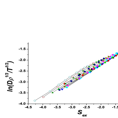
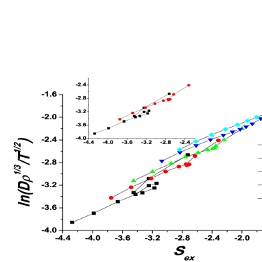
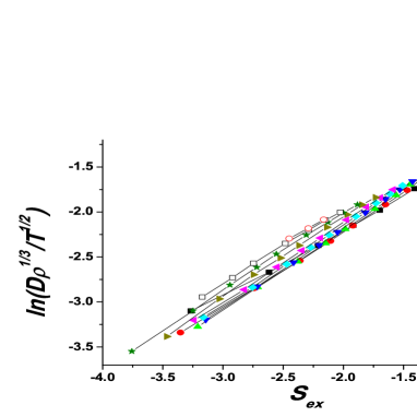
Figure 10: (Color online). Rosenfeld relation for RSS along (a) isochors, (b) isotherms, and (c) isobars.

This observation makes evident that Rosenfeld relation is valid only along the trajectories without anomalous behavior.

V V. Conclusions

In conclusion, in the present article we carry out a molecular dynamics study of the core-softened system (RSS) and show that the existence of the water-like anomalies in this system depends on the trajectory in $P-\rho-T$ space along which the behavior of the system is studied. For example, diffusion and structural anomalies are visible along isotherms, but disappears along the isochores and isobars, while density anomaly exists along isochors. We analyze the applicability of the Rosenfeld entropy scaling relations to this system in the regions with the water-like anomalies. It is shown that the validity of the of Rosenfeld scaling relation for the diffusion coefficient also depends on the trajectory in the $P-\rho-T$ space along which the kinetic coefficients and the excess entropy are calculated. In particular, it is valid along isochors and isobars, but it breaks down along isotherms. The breakdown of the Rosenfeld relation along isotherms can be explained in the following way. The regions of different anomalies do not coincide with each other. In particular, in the case of core-softened fluids the diffusion anomaly region is located inside the structural anomaly one. It means that there are some regions where the diffusion is still normal while the excess entropy is already anomalous. But this kind of behavior can not be consistent with the Rosenfeld scaling law.

- (1) P. Debenedetti, J. Phys.: Condens. Matter 15, R1669 (2003).
- (2) S. V. Buldyrev, G. Franzese, N. Giovambattista, G. Malescio, M. R. Sadr-Lahijany, A. Scala, A. Skibinsky, and H. E. Stanley, Physica A 304, 23 (2002).
- (3) C. A. Angell, Annu. Rev. Phys. Chem. 55, 559 (2004).
- (4) P. G. Debenedetti, Metastable Liquids: Concepts and Principles (Princeton University Press, Princeton, 1998).
- (5) V. V. Brazhkin. S. V. Buldyrev, V. N. Ryzhov, and H. E. Stanley [eds], New Kinds of Phase Transitions: Transformations in Disordered Substances [Proc. NATO Advanced Research Workshop, Volga River] (Kluwer, Dordrecht, 2002).
- (6) J. R. Errington and P. G. Debenedetti, Nature (London) 409, 18 (2001).
- (7) P.A. Netz, F.V. Starr, H.E. Stanley, and M.C. Barbosa, J. Chem. Phys. 115, 318 (2001).
- (8) O. Mishima and H. E. Stanley, Nature 396, 329 (1998).
- (9) C.A. Angell, E.D. Finch, and P. Bach, J. Chem. Phys. 65, 3063 (1976).
- (10) H. Thurn and J. Ruska, J. Non-Cryst. Solids 22, 331 (1976).
- (11) G.E. Sauer and L.B. Borst, Science 158, 1567 (1967).
- (12) F.X. Prielmeier, E.W. Lang, R.J. Speedy, H.-D. Lüdemann, Phys. Rev. Lett. 59, 1128 (1987).
- (13) F.X. Prielmeier, E.W. Lang, R.J. Speedy, H.-D. Lüdemann, B. Bunsenges, Phys. Chem. 92, 1111 (1988).
- (14) L. Haar, J. S. Gallagher, G. S. Kell, NBS/NRC Steam Tables. Thermodynamic and Transport Properties and Computer Programs for Vapor and Liquid States of Water in SI Units, Hemisphere Publishing Co., Washington DC, 1984, pp. 271-276.
- (15) A. Scala, F. W. Starr, E. LaNave, F. Sciortino and H. E. Stanley, Nature 406, 166 (2000).
- (16)
- (17) J. R. Errington, Th. M. Truskett, J. Mittal, J. Chem. Phys. 125, 244502 (2006).
- (18) J. Mittal, J. R. Errington, Th. M. Truskett J. Chem. Phys. 125, 076102 (2006).
- (19) Pol Vilaseca and Giancarlo Franzese, arXiv: 1005.1041v1.
- (20) Pol Vilaseca and Giancarlo Franzese, J. Chem. Phys., 133, 084507 (2010).
- (21) P. C. Hemmer and G. Stell, Phys. Rev. Lett. 24, 1284(1970).
- (22) G. Stell and P. C. Hemmer, J. Chem. Phys. 56, 4274 (1972).
- (23) G. Malescio, J. Phys.: Condens. Matter 19, 07310 (2007).
- (24) E.Velasco, L. Mederos, G. Navascues, P. C. Hemmer, and G. Stell, Phys. Rev. Lett. 85, 122 (2000).
- (25) P. C. Hemmer, E.Velasko, L. Mederos, G. Navascues, and G. Stell, J. Chem. Phys. 114, 2268 (2001).
- (26) M. R. Sadr-Lahijany, A. Scala, S. V. Buldyrev and H. E. Stanley, Phys. Rev. Lett. 81, 4895 (1998).
- (27) M. R. Sadr-Lahijany, A. Scala, S. V. Buldyrev and H. E. Stanley, Phys. Rev. E 60, 6714 (1999).
- (28) P. Kumar, S. V. Buldyrev, F. Sciortino, E. Zaccarelli, and H. E. Stanley, Phys. Rev. E 72, 021501 (2005).
- (29) L. Xu, S. V. Buldyrev, C. A. Angell, and H. E. Stanley, Phys. Rev. E 74, 031108 (2006).
- (30) E. A. Jagla, J. Chem. Phys. 111, 8980 (1999); E. A. Jagla, Phys. Rev. E 63, 061501 (2001).
- (31) F. H. Stillinger and D. K. Stillinger, Physica (Amsterdam) 244A, 358 (1997).
- (32) A. B. de Oliveira, P. A. Netz, T. Colla, and M. C. Barbosa, J. Chem. Phys. 124, 084505 (2006).
- (33) A. B. de Oliveira, P. A. Netz, T. Colla, and M. C. Barbosa, J. Chem. Phys. 125, 124503 (2006).
- (34) P. A. Netz, S. Buldyrev, M. C. Barbosa and H. E. Stanley, Phys. Rev. E 73, 061504 (2006).
- (35) A. B. de Oliveira, M. C. Barbosa, and P. A. Netz, Physica A 386, 744 (2007).
- (36) J. Mittal, J. R. Errington, and T. M. Truskett, J. Chem. Phys. 125, 076102 (2006).
- (37) H. M. Gibson and N. B. Wilding, Phys. Rev. E 73, 061507 (2006).
- (38) P. Camp, Phys. Rev. E 71, 031507 (2005).
- (39) A. B. de Oliveira, G. Franzese, P. A. Netz, and M. C. Barbosa, J. Chem. Phys. 128, 064901 (2008).
- (40) L. Xu, S. Buldyrev, C. A. Angell, and H. E. Stanley, Phys. Rev. E 74, 031108 (2006).
- (41) A. B. de Oliveira, P. A. Netz, and M. C. Barbosa, Euro. Phys. J. B 64, 481 (2008).
- (42) A. B. de Oliveira, P. A. Netz, and M. C. Barbosa, arXiv:0804.2287v1.
- (43) Yu. D. Fomin, N. V. Gribova, V. N. Ryzhov, S. M. Stishov, and Daan Frenkel, J. Chem. Phys. 129, 064512 (2008).
- (44) V. N. Ryzhov and S. M. Stishov, Zh. Eksp. Teor. Fiz. 122, 820 (2002)[JETP 95, 710 (2002)].
- (45) V. N. Ryzhov and S. M. Stishov, Phys. Rev. E 67, 010201(R) (2003).
- (46) Yu. D. Fomin, V. N. Ryzhov, and E. E. Tareyeva, Phys. Rev. E 74, 041201 (2006).
- (47) N. V. Gribova, Yu. D. Fomin, Daan Frenkel, V. N. Ryzhov, Phys. Rev. E 79, 051202 (2009).
- (48) Daan Frenkel and Berend Smit, Understanding molecular simulation (From Algorithms to Applications), 2nd Edition (Academic Press), 2002.
- (49) D. Frenkel and A. J. Ladd, J. Chem. Phys. 81, 3188 (1984).
- (50) Ya. Rosenfeld, Phys. Rev. A, 15, 2545 (1977).
- (51) Ya. Rosenfeld, J. Phys.: Condens. Matter 11, 5415 (1999).
- (52) R. Sharma, S. N. Chakraborty, and Ch. Chakravartya J. Chem. Phys. 125, 204501 (2006).
- (53) A. B. de Oliveira, E. A. Salcedo Torres, Ch. Chakravarty, M. C. Barbosa, arXiv:1002.3781 (2010).
- (54) Yu. D. Fomin, V. N. Ryzhov, and N. V. Gribova, Phys. Rev. E 81,061201 (2010).
- (55) A. Samanta, Sk. Musharaf Ali, S. K. Ghosh, J. Chem. Phys. 123, 084505 (2005).
- (56) J. J. Hoyt, Mark Asta, and Babak Sadigh, Phys. Rev. Lett. 85, 594 (2000).
- (57) A. Samanta, Sk. Musharaf Ali, and S. K. Ghosh, Phys. Rev. Lett. 87, 245901 (2001).
- (58) A. Samanta, Sk. Musharaf Ali, and S. K. Ghosh, Phys. Rev. Lett. 92, 145901 (2004).
- (59) M. Agarwal, A. Ganguly, and Ch. Chakravarty J. Phys. Chem. B, 113, 15284 (2009).
- (60) M. Agarwal and Ch. Chakravarty, Phys. Rev. E, 79, 030202(R) (2009).
- (61) Zh. Yan, S. V. Buldyrev, and H. Eu. Stanley, Phys. Rev. E, 78, 051201 (2008).
- (62) T. Goel, Ch. N. Patra, T. Mukherjee, and Ch. Chakravarty, J. Chem Phys. 129, 164904 (2008).
- (63) W.P. Krekelberg, T. Kumar, J. Mittal, J.R. Errington and T.M. Truskett, Phys. Rev. E 79 031203 (2009).
- (64) M. J. Pond, W. P. Krekelberg, V. K. Shen, J. R. Errington and Th. M. Truskett, J. Chem. Phys. 131, 161101 (2009).
- (65) Yu. D. Fomin and V.N. Ryzhov, arXiv:1008.0939v1 (2010).