A Systematic Study of Electronic Structure from Graphene to Graphane

Abstract

While graphene is a semi-metal, a recently synthesized hydrogenated graphene called graphane, is an insulator. We have probed the transformation of graphene upon hydrogenation to graphane within the framework of density functional theory. By analyzing the electronic structure for eighteen different hydrogen concentrations, we bring out some novel features of this transition. Our results show that the hydrogenation favours clustered configurations leading to the formation of compact islands. The analysis of the charge density and electron localization function (ELF) indicates that as hydrogen coverage increases the semi-metal turns into a metal showing a delocalized charge density, then transforms into an insulator. The metallic phase is spatially inhomogeneous in the sense, it contains the islands of insulating regions formed by hydrogenated carbon atoms and the metallic channels formed by contiguous bare carbon atoms. It turns out that it is possible to pattern the graphene sheet to tune the electronic structure. For example removal of hydrogen atoms along the diagonal of the unit cell yielding an armchair pattern at the edge gives rise to a band gap of 1.4 eV. We also show that a weak ferromagnetic state exists even for a large hydrogen coverage whenever there is a sublattice imbalance in presence of odd number of hydrogen atoms.

I Introduction

Carbon is regarded as one of the most versatile elements in the periodic table forming a wide variety of structures such as three dimensional sp³ bonded solids like diamond, sp² hybridized two dimensional systems like graphene and novel nano structures like fullerenes and nanotubes. The electronic structure and the physical properties of these carbon based materials are turning out to be exotic smalley . Although the existence and the properties of three dimensional allotrope, graphite containing weakly coupled stacks of graphene layers were well known wallace , the experimental realization of a monolayer graphene, brought forth a completely different set of novel properties gaim ; castro-phys . The triangular bipartite lattice of graphene leads to the electronic structure having a linear dispersion near the Dirac points. The low energy behaviour of such two dimensional electrons in graphene has been a subject of intense experimental and theoretical activity exploring the electronic, magnetic, mechanical, transport properties etc. For a recent review the reader is referred to Castro Neto et. al.  castro .

Although graphene is considered as a prime candidate for many applications, the absence of a band gap is a worrisome feature for the applications to the solid state electronic devices. In the past, several routes have been proposed to open a band gap route1 ; route2 ; route3 . The most interesting one is the recent discovery of a completely hydrogenated graphene sheet named as graphane. Graphane was first predicted by Sofo et. al. sofo on the basis of electronic structure calculations and has been recently synthesized by Elias et. al.  elias . The experimental work also showed that the process of hydrogenation is reversible, making graphane a potential candidate for hydrogen storage systems. Since upon hydrogenation, graphene, a semi-metal turns into an insulator, it is a good candidate for investigating the nature of metal insulator transition (MIT).

There are few reports investigating the electronic structure of graphene sheets as a function of hydrogen coverage leading to the opening of a bandgap. Most of these are restricted to a small number of hydrogen atoms. The electronic structure of hydrogen adsorbed on graphene has been investigated using density functional theory (DFT) by Boukhvalov et. al.boukhvalov and Casolo et. al. casolo . Their results support the use of graphene as a hydrogen storage material. Their work also shows that the thermodynamically and kinetically favoured structures are those that minimize the sublattice imbalance. Flores et. al. have investigated the role of hydrogen-frustration in graphane like structures using ab-initio methods and reactive classical molecular dynamics flores . The stability trends in small clusters of hydrogen on graphene have been discussed in a recent review roman . A recent work by Zhou et. al. zhou predicted a new ordered ferromagnetic state obtained by removing hydrogen atoms from one side of the plane of graphane. Recently, Wu et. al. Wu have reported implications of selective hydrogenation by designing an array of triangular carbon domains separated by hydrogenated strips. The electronic structure of the interface between graphene and the hydrogenated part has been investigated by Schmidt and Loss sc-loss . They show the existence of edge states for zigzag interface having strong spin orbit interaction. An interesting experimental work using scanning tunnelling microscopy, by Hornekær et.al horneka1 ; horneka2 demonstrates clustering of hydrogen atoms on graphite surface. The work shows that there is vanishingly small adsorption barrier for hydrogen in the vicinity of already adsorbed hydrogen atoms. The question of the effect of defect on the electronic structure of atomic hydrogen has been addressed by Duplock et.al dup within the density functional theory. They show that the electronic gap state associated with the adsorbed hydrogen is very sensitive to the presence of defect such as Stone-Wales defect. The localization behaviour of disordered graphene by hydrogenation has been reported within the tight binding formalism bang . The potential of hydrogenated graphene nanoribbons for spintronics applications has been investigated within DFT, by Soriano et.al soriano . The defect and disorder induced magnetism in graphene (including adsorbed hydrogen as a defect) has been studied by Yazyev, Yazyev and Helm mostly using Hubbard Hamiltonian and DFT ya1 ; ya2 ; ya3 . Theoretical investigations have also been carried out for a single hydrogen defect on graphane sheet using GW method GW , and for one and two vacancies in graphane pujari using DFT. It has been shown that interaction between adatoms in hydrogenated graphene is long range and its nature is dependant on which sublattice the adatoms reside shy . The result suggests that the adatoms tend to aggregate. A very recent work explores a formation of quantum dots as small island of graphene in graphane host singh-nm .

In the present work, we investigate some aspects of graphene - graphane transition by probing the electronic structure of hydrogenated graphene. The objective of our work is to understand the evolution of the electronic structure upon hydrogenation and gain some insight into the way band gap opens. Therefore we have carried out extensive calculations for eighteen different hydrogen coverages between graphene (0% hydrogen coverage) and graphane (100% hydrogen coverage) within the framework of DFT. Our results suggest that the hydrogenation in graphene takes place via clustering of hydrogens. Analysis based on density of states (DOS) indicates that before the gap opens (as a function of hydrogen coverage) the hydrogenated graphene sheet acquires a metallic character. This metallic state is spatially inhomogeneous in the sense, it consists of insulating regions of hydrogenated carbon atoms surrounded by the conducting channels formed by the bare carbon atoms. We also show that it is possible to tune the electronic structure by the selective decoration of hydrogen atoms to achieve semiconducting or metallic state.

In the next section we present the computational details, followed by results and discussions.

II Computational Details

The calculations have been performed using a plane-wave projector augmented wave method based code, VASP vasp . The generalized gradient approximation as proposed by Perdew, Burke and Ernzerhof gga2 has been used for the exchange-correlation potential. The convergence of binding energies with respect to the size of the supercell has been checked using three different sizes, viz., 5 $\times$ 5, 6 $\times$ 6 and 7 $\times$ 7 containing 50, 72 and 98 carbon atoms for the case of 50% hydrogen coverage. The binding energy per atom changes by about 0.05 eV (a percentage change of 0.06%) in going from 5 $\times$ 5 to 7 $\times$ 7. Therefore we have chosen a 5 $\times$ 5 unit cell for the coverage upto 50% of hydrogen and 6 $\times$ 6 for the higher coverages. This choice is consistent with the one used by Lebègue et.al GW . In order to obtain adequate convergence in the density of states, we have carried out calculations on different $k$ grids. It was found that at least 9 $\times$ 9 $k$ grid was required during geometry optimization for an acceptable convergence. However, a minimum of 17 $\times$ 17 $k$ grid was necessary for obtaining an accurate DOS. The convergence criterion used for the total energy and the force are 10^-5 eV and 0.005 eV/Å respectively.

All the calculations have been performed on the chair conformer configuration where hydrogen atoms are attached to carbon atoms alternatively on opposite sides of the plane. This is known to be a lower energy configuration as compared to the boat conformer sofo ; GW .

III Results and discussion

Table 1: Shifted binding energies (BE) for different configuration of 20% coverage (10H + 50C). The binding energy of the most stable structure is the reference(zero) level. The more negative binding energy means more unstable structure.

20% Hydrogen Coverage
Configuration	BE (total cell) (eV)
Random placement of hydrogens	-9.32
Five hydrogen pairs placed separately	-4.29
Hydrogens placed along the diagonal of the cell	-2.85
Two clusters of seven and three hydrogens	-2.15
A single hydrogen isolated from the cluster of nine hydrogens	-1.77
One compact cluster	0.0

In order to decide the minimum energy positions for hydrogen atoms, following procedure has been adopted. Upto 20% coverage of hydrogen, we have carried out the geometry optimization for two different configurations of hydrogen atoms, first by placing the hydrogen atoms randomly and second by placing the hydrogen atoms contiguously, so as to form a compact cluster of hydrogenated carbon atoms. It turns out that, in all the cases, the configuration forming the compact cluster of the hydrogen atoms is energetically favoured. In order to assess the relative stability of different patterns we have calculated six different patterns for 20% coverage case as shown in table 1. The binding energy of the most stable structure is the reference level. The more negative binding energy means more unstable structure.

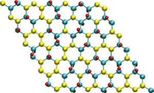
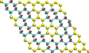
(a)                                            (b)

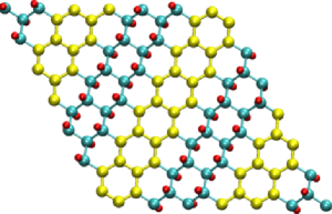
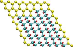
(c)                                            (d)

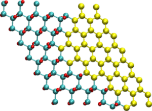
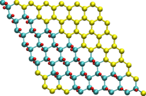
(e)                                            (f)

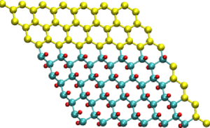
(g)

Figure 1: (Colour online) Different hydrogen decorations for 50% concentration. In figure, yellow (in print light shaded) balls are bare carbon atoms, turquoise (in print darker shades) balls are hydrogenated carbons and red (in print dark small) balls are hydrogen atoms.

We note that the compact cluster configuration is the lowest in energy and is lower by 0.9 eV/H atom compared to the energy of the configuration with randomly placed hydrogen atoms. Thus our geometry optimization shows a preference for hydrogens to decorate the graphene lattice in a contiguous and compact manner. In order to assess the validity of this process for the larger coverages and to understand the influence of different edge patterns like zigzag and arm chair, we have considered seven different patterns for 50% coverage, as shown in figure 1. These calculations have been carried out on a larger unit cell containing 98 atoms of carbon. Although a compact cluster configuration is energetically preferred one, there are different ways in which the hydrogens can be placed yielding a compact geometry. The seven cases considered are : 1) Randomly distributed hydrogens (figure 1(a)), 2) A chain of bare carbon atoms (figure 1(b)), 3) Three separated clusters as shown in (figure 1(c)), 4) A single cluster having zigzag interface and with one line of bare carbon atoms at the two side edges (figure 1(d)), 5) A mixture of armchair and zigzag pattern at the interface (figure 1(e)), 6) A armchair pattern at the interface (figure 1(f)) and 7) A zigzag pattern at the interface (figure 1(g)).

Table 2: Shifted binding energies (BE) for different configuration of 50% coverage as shown in figure 1. The binding energy of the most stable structure is the reference(zero) level. The more negative binding energy means more unstable structure.

50% Hydrogen Coverage on 98 Carbon cell
Configuration	BE (total cell) (eV)
Random placement of hydrogens (figure 1(a))	-23.29
Chain of connecting bare Carbon atoms (figure 1(b))	-3.65
Three separated islands (figure 1(c))	-3.25
Zigzag interface with a line of bare carbon atoms at the two side edges (figure 1(d))	-2.46
Compact mixed (zigzag & armchair) interface (figure 1(e))	-1.66
Compact armchair interface (figure 1(f))	-1.43
Compact zigzag interface (figure 1(g))	0.0

In the zigzag case each hexagonal ring at the edge has three hydrogenated carbons and three empty carbons. An armchair pattern consists of only two hydrogenated carbons at the edge. The binding energies for all these seven structures (shown in figure 1) are compared in the table 2. Even among the islands, the ‘most compact’ one (having minimum surface area of covered hydrogens) has the highest binding energy. By the most compact, we mean an island of hydrogenated carbons which covers the minimum area. We have discussed more details about the zigzag and arm chair patterned configurations in section III.2.

The tendency to form the compact cluster can be understood by noting that the hydrogen atom placed on the top of an bare carbon atom pulls up the carbon atom above the plane by 0.33 Å and deforms the surrounding lattice points also. Therefore it costs less energy to place an extra hydrogen atom nearest to the existing cluster, since the number of strained bonds is less compared to the case where the hydrogen atom is placed away from the cluster. In the latter case the entire neighbourhood is deformed. Our results are consistent with the work of Hornekær et al  horneka1 .

Table 3: Shifted binding energies (BE) (eV) and the magnetic moments($\mu_{B}$) of 4 hydrogen vacancies. The binding energy of the most stable structure is the reference(zero) level. The more negative binding energy means more unstable structure.

92% Hydrogen Coverage (4 vacancies)
Configuration	BE (total cell)	Magnetic Moment
Random	-5.50	4.0
3H on one hexagon and 1 on other	-2.09	1.82
2H pairs placed on different hexagons	-0.11	nil
Compact single island	0.0	nil

We have also carried out a similar analysis for the case of four hydrogen vacancies in graphane. The calculations for various configurations have been carried out with spin polarization. The calculated binding energies and the magnetic moments are tabulated in table 3. The four configurations considered are 1) 4 hydrogen atoms removed randomly, 2) 3 hydrogen atoms removed from one hexagon and 1 from other, 3) 2 hydrogen atom pairs removed from different hexagons and 4) 4 hydrogens removed from a single hexagon (compact). We observe that the structure having a compact form of vacancies has the highest binding energy. The magnetic moment is about 2 for the lattice imbalance case. It is fruitful to recall Lieb’s theorem which states that for a bipartite lattice (one electron per site) the spin S of the ground state is 1/2 $\times$ (the lattice imbalance) lieb . The magnetic moment seen in the case of random placement is just the sum of the isolated moments of hydrogen atoms, essentially a non interacting case.

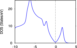
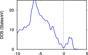
(a) Graphene                           (b) 4% hydrogen

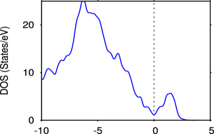
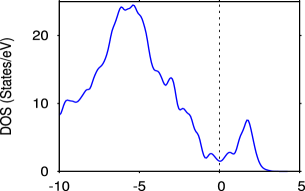
(c) 16% hydrogen                           (d) 20% hydrogen

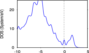
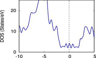
(e) 30% hydrogen                           (f) 50% hydrogen

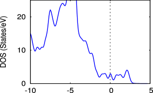
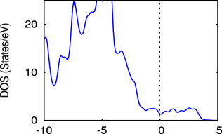
(g) 60% hydrogen                           (h) 70% hydrogen

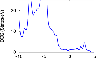
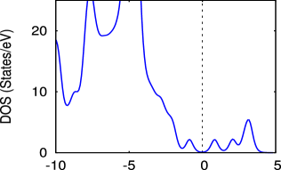
(i) 80% hydrogen                           (j) 85% hydrogen

Figure 2: (Colour online) The total DOS for hydrogenated graphene for various hydrogen concentrations below 90%. The zero of the energy is taken at the Fermi level and is marked by a vertical line. X axis denotes $E-E_{f}$.

Now we discuss the total DOS for different hydrogen coverages which are shown in figure 2 and 3. All the DOS are for the non spin polarised cases. The geometry used is for the minimum energy configuration (compact cluster of hydrogen atoms). In both the figures the plots are shown in a restricted region to enhance the clarity near the Fermi energy. The effect of addition of a small concentration of hydrogen in the V-shape DOS near E_f can be seen from figure (2(b) to 2(d)). It can be noted that the characteristic V shape valley seen in figure 2(a) is due to peculiar sp² bonded carbon atoms in graphene, and the addition of hydrogen atoms immediately distorts the symmetry producing the deformation in the DOS. Thus in this region, the DOS is modified by additional localized $\sigma$-p_z bonds between the hydrogen and carbon.

As the hydrogen coverage increases there is a significant increase in the value of DOS at the Fermi level. The process of hydrogenation is accompanied by the change in the geometry. The hydrogenated carbon atoms are now moved out of the graphene plane, in turn the lattice is distorted and the symmetry is broken. As a consequence, more and more $k$ points in the Brillouin zone contribute to the DOS near Fermi level, the increase being rather sharp after 20% coverage. The region ranging from 30% coverage to about 60% coverage is characterized by the finite DOS of the order of 2.5/eV near the Fermi energy. As we shall discuss this region can be described as having metallic character with delocalized charge density.

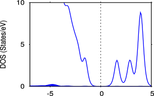
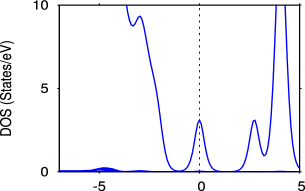
(a) 92% hydrogen                           (b) 94% hydrogen

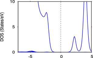
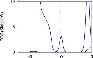
(c) 96% hydrogen                           (d) 98% hydrogen

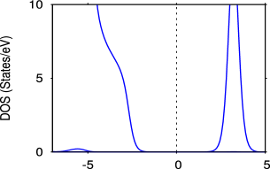
(e) Graphane

Figure 3: (Colour online) The total DOS for hydrogenated graphene for various hydrogen concentrations above 90%. The zero of the energy is taken at the Fermi level and is marked by a vertical line. X axis denotes $E-E_{f}$.

Now we complete the discussion of DOS by presenting the cases of hydrogen coverages greater than 90%. In figure 3 we show the density of states obtained by the removal of one - four hydrogen atoms in a unit cell containing fifty carbon atoms. Clearly one and three hydrogen vacancies (i.e 98% hydrogen and 94% hydrogen respectively) induce states on the Fermi level while two and four hydrogen vacancies (i.e 96% hydrogen and 92% hydrogen respectively) do not induce any state at the Fermi level (See the discussion of hydrogen imbalance later). For a small number of vacancies these are $\pi$ bonded states localized on bare carbon atoms.

In summary, it is possible to discern, rather broadly, three regions of hydrogen coverage. A low concentration region, where the DOS undergo the distortions due to loss of lattice symmetry of the system, intermediate concentration region where a metallic-like phase is seen and a vary high concentration region where most of the carbon atoms are hydrogenated and vacancy gives rise to midgap states.

As discussed before, our calculations show the presence of localized states in the DOS for a very low hydrogen coverage as well as for very high hydrogen coverage (midgap states). These DOS show a pattern of peak or a valley at E_f (in case of low coverage) and at the centre of the gap (in case of high coverage). The reasons can be attributed to the existence of sublattice imbalance. If the difference of hydrogen atoms on the two sides of the sheet is odd then it leads to a peak. Hence by adding impurities one by one to graphane we get a sequence of midgap states. This is in consistent with the work of Casolo et al  casolo . Interestingly this feature is also retained for the intermediate coverages of hydrogen (where we get a finite DOS at the Fermi level) when the sub lattice imbalance of hydrogen is one, e.g., in figure 2(e), 2(f) and 2(g), we see the peaks at Fermi level. As we shall see in section III.1 this feature has an implication for the magnetic behaviour of the system.

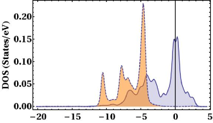
Figure 4: (Colour online) Site projected DOS for hydrogenated carbon sites (dotted line) and bare carbon sites (continuous line) for hydrogen coverage of 40%. Almost all the contribution comes from the $p_{z}$ which has been showed in the figure. Note that only bare carbon atoms contribute to the DOS at Fermi level.

In order to bring out the difference between the local electronic structure of the bare carbon atoms and the hydrogenated carbon atoms, we have analyzed the site projected DOS for all the cases. In figure 4, we show site projected DOS for 40% hydrogen coverage depicting the contributions from a hydrogenated carbon site and a bare carbon site. Quite clearly, the contribution around the Fermi level comes from the $p_{z}$ orbitals of bare carbon atoms only. This is a general feature for all the systems investigated. It may be emphasized that in pure graphene all the carbon atoms contribute to a single $k$ point (Dirac point). In contrast to this, upon hydrogenation, only bare carbon atoms contribute to the DOS at Fermi energy, and they do so at many $k$ points of the Brillouin zone. As the concentration increases further (above 80%), there are too few bare carbon atoms available for the formation of delocalized $\pi$ bonds. The value of DOS approaches zero and a gap is established with a few mid gap states.

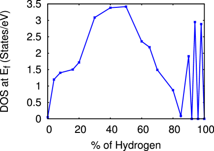
Figure 5: (Colour online) Variation of the value of DOS at the Fermi level as a function of hydrogen coverage.

The evolution towards the metallic state can be better appreciated by examining the variation in the value of DOS at the Fermi level which is shown in figure 5. A clear rise in DOS is seen after 20% hydrogen concentration peaking around 3.5 eV at 50% concentration. This rise is due to the increasing number of $k$ points contributing to the Fermi level, as inferred from the analysis of the individual bands. Evidently, over a significant range of concentration, the value at Fermi level is more than 2/eV. The decline seen after 60% is because of the reduction in the number of bare carbon atoms. The character of the DOS changes after about 80%. The value of the DOS at the Fermi level oscillates between zero and some finite value. It is most convenient to describe this region as graphane with defects by the removal of a few hydrogen atoms giving rise to mid gap states. The nature and the placement of the induced states is dependent on the number of hydrogen atoms removed.

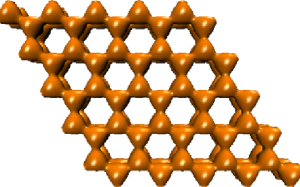
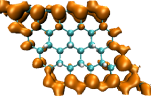
(a) Graphene                           (b) 40% hydrogen

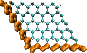
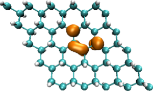
(c) 70% hydrogen                           (d) 92% hydrogen

Figure 6: (Colour online) Isosurfaces of charge densities of bands near the Fermi level (see text). For comparison, the charge density of graphene at Dirac point is also shown.

It may be emphasized that the presence of states around the Fermi level giving finite DOS does not guarantee that the system is metallic unless we examine the nature of localization of the individual states. Therefore we have examined the energy resolved charge densities of the states near the Fermi level and the electron localization function (ELF). The energy resolved charge densities are obtained by summing the charge densities of all the k points contributing in the small energy region near E_f. Therefore, the charge densities shown in (figure 6) for 40%, 70% and 92% hydrogen coverages specifically brings out the nature of the states near E_f. A particularly striking feature is the formation of two spatially separated regions as seen in figure 6(b) and 6(c). The hydrogenated regions hardly contribute to the charge density giving rise to the insulating regions surrounded by the $\pi$ bonded bare carbon atoms forming conducting regions. This feature is also seen for the higher concentrations upto 70%. It may be emphasized that the topology in this range of concentrations (30%-70%) shares a common feature namely, there is a contiguous region formed by the bare carbon atoms. It may be pointed out that the contiguous charge density is attributed to the favoured configuration of compact cluster formation . The change in the character of the state at 90% and above is also evident in figure 6(d). There are insufficient number of bare carbon atoms to form contiguous regions. As a consequence, these carbon atoms form localized bonds giving rise to mid gap states noted earlier.

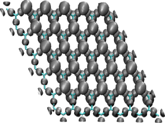
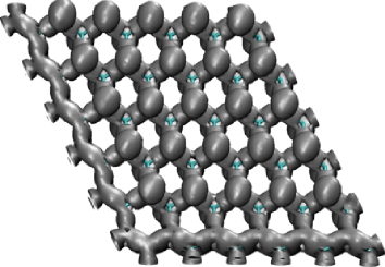
(a)                                            (b)

Figure 7: (Colour online) ELF plots with two different isosurface values for 70% hydrogen concentration. Figure (a) shows for isosurface value 0.75 and figure (b) shows for isosurface value 0.62 .

The degree of delocalization of an electron of the system can be understood by examining the electron localization function as follows. For a single determinantal wave function built from Kohn-Sham orbitals, $\psi_{i}$, the ELF is defined as, becke

$$\chi_{{\rm ELF}}=[1+{(D/D}_{h}{)}^{2}]^{-1},$$ (1)

where

$$D_{h} = (3/10){(3{\pi}^{2})}^{5/3}{\rho}^{5/3},$$ (2)

$$D = (1/2)\sum_{i}{\ |{\bm{\nabla}\psi_{i}}|}^{2}-(1/8){|{\bm{\nabla}\rho}|}^{2}/\rho,$$ (3)

with $\rho\equiv\rho({\bf r})$ being the electron density. D is the excess local kinetic energy density due to Pauli repulsion and D_h is the Thomas–Fermi kinetic energy density. The numerical values of $\chi_{{\rm ELF}}$ are conveniently normalized to a value between zero and unity. A value of 1 represents a perfect localization of the charge, while the value for the uniform electron gas is 0.5. Typically, the existence of an isosurface of a high value of $\chi_{{\rm ELF}}$ say, $\geq 0.70$, signifies a localized bond.

We have examined the isosurfaces of ELF for various values between 0.5 and 1.0. The isosurface for a typical value 0.75, is shown in figure 7(a) for 70% coverage. It can be seen that for this high value isosurface exists mainly along carbon-hydrogen bonds ($\sigma$-p_z). The existence of localized $\sigma$ bonds between the bare carbon atoms can also be noticed. In figure 7(b) we show the isosurface for the value of 0.62. The figure shows a continuous surface covering all the bare carbon atoms. This signifies the delocalized nature of the charge density arising out of $\pi$ bonds formed by p_z orbitals. We have analyzed the ELF for all the coverages. The above features are seen for the coverages from 30% to 80%. Thus the analysis of ELF confirms the delocalized nature of the charge density near the Fermi level for the concentration from 30% to 80%.

III.1 Magnetism

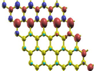
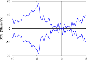
(a)                                            (b)

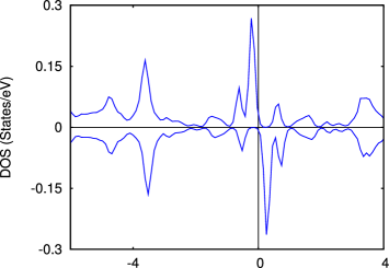
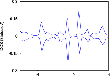
(c)                                            (d)

Figure 8: (Colour online) (a) Spin density, (b) total DOS, (c) and (d) site projected ($p_{z}$ only) DOS for two bare carbon atoms from two different sublattices. X axis of the plots denotes $E-E_{f}$. This figure is for 50% hydrogen coverage.

The existence of a peak at Fermi level in the non spin polarized calculation is an indication of Stoner instability that may lead to a more stable spin polarized solution. As an example we have analyzed the case of 50% hydrogen coverage which shows a peak in the DOS at the Fermi level. When we allow spin polarization in our calculations, indeed we find a stable ferromagnetic solution, e.g., for 50% hydrogen coverage we get a total magnetic moment $\sim$ 1 $\mu_{B}$ per unit cell as reflected in the spin density plot shown in figure 8(a). However, the exchange splitting seen on the bare carbon atoms is rather small and is expected to survive only at a very low temperature. This fragile nature of magnetism is clearly indicated by the collapse of magnetic moment with a smearing width of 0.08 eV. The site projected DOS for two bare carbon atoms belonging to two different sublattices along with the spin density plots are shown in figure (8(c) and 8(d)). Carbon atom belonging to one sublattice shows a spin-polarized behaviour whereas the other sublattice carbon atom has an energy gap in the electronic spectrum. This sublattice effect is similar to what is observed in case of graphene nanoribbons bhandary .

III.2 Tuning the electronic structure with hydrogenation

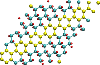
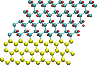
(a)                                            (b)

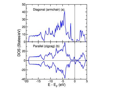
(c)

Figure 9: (Colour online) Decoration of hydrogen (a) along the diagonal of the unit cell and (b) along the edge of the unit cell. In figure, yellow (in print light shaded) balls are bare carbon atoms, turquoise (in print darker shades) balls are hydrogenated carbons and red (in print dark small) balls are hydrogen atoms. (c) DOS plots for the two cases. The lone atoms seen are from repeating super cells

Now we bring in another interesting aspect of hydrogenation brought out by our calculations. Our results indicate that it is possible to pattern the graphene lattice with hydrogen and tune the electronic structure. In figure 9(a), the patterning is done by removing the hydrogen atoms along the diagonal of the unit cell where as in figure 9(b) the hydrogen atoms are removed parallel to one edge of the unit cell. The horizontal pattern is more stable than the diagonal pattern by 0.04 eV/H atom. The corresponding DOS are shown in figure 9(c) where a dramatic difference is seen. The diagonal pattern shows a clear band gap of 1.4 eV whereas the horizontal pattern shows finite DOS along with a magnetic solution. A close inspection of the geometry reveals an analogy with graphene nano ribbons (GNR). The diagonal pattern resembles an armchair GNR with a chain of hexagons while the horizontal pattern is analogous to a zigzag GNR with a width of 3 rows in this particular case. The corresponding DOS also resemble the electronic structure of an armchair (zigzag) GNR with a semiconducting (metallic) nature Loui . It is a reasonable conjecture that the band gaps of the patterned system can be tuned by controlling the width of the bare carbon channels analogous to the case of armchair GNR where the band gap decreases as the width of GNR is increased.

IV Concluding Remarks

In conclusion, our detailed density functional investigations have revealed some novel features of graphene-graphane metal-insulator transition. As the hydrogen coverage increases, graphene with a semi metallic character turns first into a metal and then to an insulator. Hydrogenation of graphene pulls the carbon atom out of the plane breaking the symmetry of pure graphene. As a consequence, many $k$ points in the Brillouin zone contribute to the DOS at the Fermi level giving rise to a metallic system. The metallic phase has some unusual characteristics: the sheet shows two distinct regions, a conducting region formed by bare carbon atoms and embedded into this region are the non conducting islands formed by the hydrogenated carbon atoms. The onslaught of insulating state occurs when there are insufficient numbers of bare carbon atoms to form connecting channels. This also means that the transition to insulating phase depends on the distribution of hydrogen atoms and will occur when the continuous channels are absent. The present work opens up the possibility of using partially hydrogenated graphene having designed patterns of conducting channels along with insulating barriers for the purpose of devices. Our results also show that it is possible to design a pattern of hydrogenation so as to yield a semiconducting sheet with a band gap much lower than that of graphane. Finally we may note that the calculation of conductivity in such a disordered system is a complex issue. The present study focusses on the evolution of the density of states to understand the change in the character of single particle orbitals as a function of hydrogen coverage. An obvious extension of this work is the study of transport properties to have a more vivid picture.

References

- [1] R.E. Smalley. Rev. Mod. Phys., 69:723, 1997.
- [2] P. R. Wallace. Phys. Rev., 71:622, 1947.
- [3] A. K. Geim and K. Novesolov. Nat. Mater., 6:183, 2007.
- [4] A. H. Castro Neto, F. Guinea, and N. M. R. Peres. Physics World., 19:33, 2006.
- [5] A. H. Castro Neto, F. Guinea, N. M. R. Peres, K. S. Novoselov, and A. K. Geim. Rev. Mod. Phys., 81:109–62, 2009.
- [6] R. M. Ribeiro, N. M. R. Peres, J. Coutinho, and P. R. Briddon. Phys. Rev. B, 78:075442, 2008.
- [7] E. Bekyarova, M. E. Itkis, P. Ramesh, C. Berger, M. Spinkle, W. A. De Heer, and R. C. Haddon. J. Am. Chem. Soc., 131:1336, 2009.
- [8] P. A. Denis, R. Faccio, and A. W. Mombru. ChemPhysChem, 10:715, 2009.
- [9] J. O. Sofo, A. S. Chaudhari, and G. D. Barber. Phys. Rev. B., 75:153401, 2007.
- [10] D. C. Elias, R. R. Nair, T. M. G. Mohiuddin, S. V. Morozov, P. Blake, M. P. Halsall, A. C. Ferrari, D. W. Boukhvalov, M. I. Katsnelson, A. K. Geim, and K. S. Novoselov. Science, 323:610–613, 2009.
- [11] D. W. Boukhvalov, M. I. Katsnelson, and A. I. Lichtenstein. Phys Rev B, 77:035427, 2008.
- [12] S. Casolo, O. M. Løvvik, R. Martinazzo, and G. F. Tantardini. J. Chem. Phys., 130:054704, 2009.
- [13] M Z S Flores, P A S Autreto, S B Legoas, and D S Galvao. Nanotechnology, 20:465704, 2009.
- [14] T Roman, W A Diño, H Nakanishi, and H Kasai. Journal of Physics: Condensed Matter, 21:474219, 2009.
- [15] J. Zhou, Q. Wang, Q. Sun, X. S. Chen, Y. Kawazoe, and P. Jena. Nano Letters, 9:3867–3870, 2009.
- [16] Menghao Wu, Xiaojun Wu, Yi Gao, and Xiao Cheng Zeng. The Journal of Physical Chemistry C, 114:139–142, 2010.
- [17] Manuel J. Schmidt and Daniel Loss. Phys. Rev. B, 81:165439, 2010.
- [18] L. Hornekær, E. Rauls, W. Xu, Ž. Šljivančanin, R. Otero, I. Stensgaard, E. Lægsgaard, B. Hammer, and F. Besenbacher. Phys. Rev. Lett., 97:186102, 2006.
- [19] L. Hornekær, Ž. Šljivančanin, W. Xu, R. Otero, E. Rauls, I. Stensgaard, E. Lægsgaard, B. Hammer, and F. Besenbacher. Phys. Rev. Lett., 96:156104, 2006.
- [20] Elizabeth J. Duplock, Matthias Scheffler, and Philip J. D. Lindan. Phys. Rev. Lett., 92:225502, 2004.
- [21] Junhyeok Bang and K. J. Chang. Phys. Rev. B, 81:193412, 2010.
- [22] D. Soriano, F. Muñoz Rojas, J. Fernández-Rossier, and J. J. Palacios. Phys. Rev. B, 81:165409, 2010.
- [23] Oleg V Yazyev. Reports on Progress in Physics, 73:056501, 2010.
- [24] Oleg V. Yazyev. Phys. Rev. Lett., 101:037203, 2008.
- [25] Oleg V. Yazyev and Lothar Helm. Phys. Rev. B, 75:125408, 2007.
- [26] S. Lebègue, M. Klintenberg, O. Eriksson, and M. I. Katsnelson. Phys. Rev. B., 79:245117, 2009.
- [27] Bhalchandra S. Pujari and D. G. Kanhere. The Journal of Physical Chemistry C, 113:21063–21067, 2009.
- [28] Andrei V. Shytov, Dmitry A. Abanin, and Leonid S. Levitov. Phys. Rev. Lett., 103:016806, 2009.
- [29] Abhishek K. Singh, Evgeni S. Penev, and Boris I. Yakobson. ACS Nano, 4:3510–3514, 2010.
- [30] G. Kresse and J. Furthmüller. Phys. Rev. B, 54:11169, 1996.
- [31] J. P. Perdew, K. Burke, and M. Ernzerhof. Phys. Rev. Lett., 78:1396, 1997.
- [32] Elliott H. Lieb. Phys. Rev. Lett., 62:1201–1204, 1989.
- [33] A. D. Becke and K. E. Edgecombe. The Journal of Chemical Physics, 92:5397–5403, 1990.
- [34] Sumanta Bhandary, Olle Eriksson, Biplab Sanyal, and Mikhail I. Katsnelson. Phys. Rev. B, 82:165405, 2010.
- [35] Young-Woo Son, Marvin L. Cohen, and Steven G. Louie. Phys. Rev. Lett., 97:216803, 2006.
- [36] W. Humphrey, A. Dalke, and K. Schulten. J. Molecular Graphics, 14:33–38, 1996.
- [37] Anton Kokalj. Computational Materials Science, 28:155 – 168, 2003.