Lattice Boltzmann study on Kelvin-Helmholtz instability: the roles of velocity and density gradients

Abstract

A two-dimensional lattice Boltzmann model with 19 discrete velocities for compressible fluids is proposed. The fifth-order Weighted Essentially Non-Oscillatory (5th-WENO) finite difference scheme is employed to calculate the convection term of the lattice Boltzmann equation. The validity of the model is verified by comparing simulation results of the Sod shock tube with its corresponding analytical solutions. The velocity and density gradient effects on the Kelvin-Helmholtz instability (KHI) are investigated using the proposed model. Sharp density contours are obtained in our simulations. It is found that, the linear growth rate $\gamma$ for the KHI decreases with increasing the width of velocity transition layer ${D_{v}}$ but increases with increasing the width of density transition layer ${D_{\rho}}$. After the initial transient period and before the vortex has been well formed, the linear growth rates, $\gamma_{v}$ and $\gamma_{\rho}$, vary with ${D_{v}}$ and ${D_{\rho}}$ approximately in the following way, $\ln\gamma_{v}=a-bD_{v}$ and $\gamma_{\rho}=c+e\ln D_{\rho}({D_{\rho}}<{D_{\rho}^{E}})$, where $a$, $b$, $c$ and $e$ are fitting parameters, and ${D_{\rho}^{E}}$ is the effective interaction width of density transition layer. When ${D_{\rho}}>{D_{\rho}^{E}}$ the linear growth rate $\gamma_{\rho}$ does not vary significantly any more. One can use the hybrid effects of velocity and density transition layers to stabilize the KHI. Our numerical simulation results are in general agreement with the analytical results [L. F. Wang, et al., Phys. Plasma 17, 042103 (2010)].

I Introduction

As a mesoscopic approach and a bridge between the molecular dynamics method at the microscopic level and the conventional numerical method at the macroscopic level, the lattice Boltzmann (LB) method Succi-Book has been successfully applied to various fields during the past two decades, ranging from the multiphase system Yeomans ; XGL1 ; Sofonea-multiphase , magnetohydrodynamics Chensy-PRL-1991 ; Succi-PRA-1991 ; CICP-2008 , reaction-diffusion system reactive-1 ; reactive-2 ; reactive-3 , compressible fluid dynamics Sunch-PRE-1998 ; Katato ; Watari ; Xu-compressible ; Xu-compressible-2 ; Xu-compressible-3 ; QuKun ; HYL , simulations of linear and nonlinear partial differential equations PDE-1 , etc. Its popularity is mainly owed to its kinetic nature kinetic nature , which makes the physics at mesoscopic scale can be incorporated easily. As a result, this approach contains more physical connotation than Navier-Stokes or Euler equations based on the continuum hypothesis. Its popularity is also owed to its linear convection term, easy implementation of boundary conditions, simple programming and high efficiency in parallel computing, etc.

The Kelvin-Helmholtz instability (KHI) occurs when two fluids flow with different tangential velocities KH-BOOK . Under the condition of the KHI, small perturbations along the interface between two fluids undergo linear PFA-1993 ; PF-1982 ; PF-1980 ; wang-pop-2009 ; wang-pop-2010 and nonlinear growth stages PRL-1999 ; PRL-2002 ; PRE-2004 ; POP-2005 ; wang-epl-2009 , and may evolve into turbulent mixing through nonlinear interactions. The KHI has attracted much attention because of its significance in both fundamental research and engineering applications HEDP . On the one hand, in fundamental research, KHI is of great importance in the fields of turbulent mixing turbulent , supernovae dynamics supernovae-1 ; supernovae-2 ; supernovae-3 , and the interaction of the solar wind with the earth’s magnetosphere earth magnet , etc. On the other hand, in engineering applications, the KHI plays a key role in small-scale mixing of Rayleigh-Taylor (RT) pop-2010-2 ; epl-2010-2 and Richtmyer-Meshkov (RM) instabilities in inertial confinement fusion (ICF) ICF-3 ; ICF-4 ; ICF-book . In the final regime of RT and RM instabilities, KHI is initiated due to the shear velocity difference at the spike tips KH-RM-RT , and, therefore, the appearance of the KHI aggravates the development of final nonlinearity of RT instability or RM instability, and quickens the process of fluid flock mixing round the interface.

In the present work, we propose a two-dimensional LB mode to simulate the KHI. The model consists of 19 discrete velocities in six directions and allows to recover the compressible Euler equations in the continuum limit. Actually, this phenomenon has been studied extensively by many researchers using experimental measurements, theoretical analysis and more recently by numerical simulations during the past decades KH-BOOK ; wang-pop-2009 ; wang-pop-2010 ; wang-epl-2009 ; HEDP ; turbulent . Those results indicate that the evolution of KHI depends on the density ratio, viscosities, surface tension, compressibility and others. Although the basic behavior of the KHI has been studied extensively, to the best of our knowledge, the use of the LB method to investigate the evolution of this phenomenon is still very limited. In this paper, with the LB method we focus on the velocity and the density gradient effects on KHI. The rest of the paper is organized as follows. In Section II, using the Chapman-Enskog analysis, we show that the current model can recover the Euler equations in the continuum limit. The numerical scheme and the validation of the model will be performed in Section III. In Section IV, we show numerical simulation results on the KHI for various widths of velocity and density transition layers. Both the two kinds of gradients effects are investigated carefully. Finally, in Section V conclusions and discussions are drawn.

II Formulation of the LB model

The model described here is inspired by the previous work of Watari and Tsutahara Watari , which is based on a multispeed approach and where the truncated local equilibrium distribution uses global coefficients.

II.1 Designing of the discrete velocity model

In the present study, we will propose a finite difference LB (FDLB) model for compressible flows. Within this scheme, the physical symmetry of hydrodynamic systems can be more conveniently recovered by the use of discrete velocity model with high spatial isotropy. For completeness, let us start with the standard LB equation, an exact lattice-based dynamical equation expressed in terms of particle streaming and the Bhatnagar-Gross-Krook (BGK) collision operator

$$f_{i}^{{}^{\prime}}(\mathbf{r}^{{}^{\prime}}+\mathbf{v}_{i}^{{}^{\prime}}\Delta t^{{}^{\prime}},t^{{}^{\prime}}+\Delta t^{{}^{\prime}})-f_{i}^{{}^{\prime}}(\mathbf{r}^{{}^{\prime}},t^{{}^{\prime}})=-\frac{1}{\tau^{{}^{\prime}}/\Delta t^{{}^{\prime}}}(f_{i}^{{}^{\prime}}-f_{i}^{(0)^{\prime}})\text{,}$$ (1)

where $f_{i}^{{}^{\prime}}$ is the distribution function along the $i$ direction, $f_{i}^{(0)^{\prime}}$ is its corresponding equilibrium distribution function, $\mathbf{r}^{{}^{\prime}}$ is the spatial coordinate, $\mathbf{v}_{i}^{{}^{\prime}}$ is the particle velocity in the $i$ direction, $\Delta t^{{}^{\prime}}$ is the time step, and $\tau^{{}^{\prime}}$ is relaxation time determining the viscosity of fluid. For the standard LB method, all the particle velocities are restricted to those that exactly link the lattice sites in unit time. In other words, there is a banding of discretizations of space and time, which is an inconvenience in the use of the standard LB model to study the thermohydrodynamic problems.

The standard LB equation can be approximately expressed as the discrete velocity Boltzmann equation

$$\frac{\partial f_{ki}^{{}^{\prime}}}{\partial{{t}^{{}^{\prime}}}}+\mathbf{v}_{ki}^{{}^{\prime}}\cdot\frac{\partial f_{ki}^{{}^{\prime}}}{\partial{{\mathbf{r}}^{{}^{\prime}}}}=-\frac{1}{{{\tau}^{{}^{\prime}}}}(f_{ki}^{{}^{\prime}}-f_{ki}^{(0)^{\prime}})\text{,}$$ (2)

where $\mathbf{v}_{ki}^{{}^{\prime}}$ represents the discrete velocity model, subscript $k$ indicates the $k$th group of the particle velocities whose speed is $v_{k}^{{}^{\prime}}$. Eq.(2) may be written in a dimensionless form by choosing three independent reference variables, the characteristic flow length scale $L_{0}$, the reference speed $c_{s}$ and the reference density $\rho_{0}$. The characteristic time $t_{0}$ can be expressed as $t_{0}=L_{0}/c_{s}$. With these reference variables, we have the following dimensionless variables

$$t=\frac{{{t}^{{}^{\prime}}}}{{{t}_{0}}}\text{, }r=\frac{{{r}^{{}^{\prime}}}}{{{r}_{0}}},\text{ }{{v}_{ki}}=\frac{v_{ki}^{{}^{\prime}}}{{{c}_{s}}}\text{, }{{f}_{ki}}=\frac{f_{ki}^{{}^{\prime}}}{{{\rho}_{0}}},\text{ }\tau=\frac{{{\tau}^{{}^{\prime}}}}{{{t}_{0}}}\text{.}$$ (3)

Consequently, we have the following dimensionless lattice Boltzmann equation

$$\frac{{\partial f_{ki}}}{{\partial t}}+\mathbf{v}_{ki}.\frac{\partial}{{\partial\mathbf{r}}}f_{ki}=-\frac{{1}}{\tau}(f_{ki}-f_{ki}^{{(0)}})\text{.}$$ (4)

To formulate a FDLB model, the next step is to chose an appropriate dimensionless discrete velocity model $\mathbf{v}_{ki}$. For a discrete velocity model described by

$$\mathbf{v}_{0}=0\text{, }\mathbf{v}_{ki}=v_{k}[\cos(\frac{{i2\pi}}{N})\text{,}\sin(\frac{{i2\pi}}{N})]\text{,}$$ (5)

the $n$th rank tensor is defined as

$$T_{\alpha_{1}\alpha_{2}...\alpha_{n}}^{(n)}=\sum\limits_{i=1}^{n}{v_{i\alpha_{1}}}v_{i\alpha_{2}}...v_{i\alpha_{n}}\text{,}$$ (6)

where $\alpha_{1}$, $\alpha_{2}$,…,$\alpha_{n}$ indicate either the $x$ or $y$ component. The tensor is isotropic if it is invariant under the coordinate rotation and the reflection. As for being isotropic, the odd rank tensors should be zero and the even rank tensors should be the sum of all possible products of Kronecker delta. In this study, the discrete velocity model with $N=6$ is used to construct a FDLB model. For this discrete velocity model it is easy find that the odd rank tensors are zero, and the even rank tensors generally have the following forms

$$\sum\limits_{i{=1}}^{{6}}{v_{ki\alpha}}v_{ki\beta}=3v_{k}^{2}\delta_{\alpha\beta}\text{,}$$ (7)

$$\sum\limits_{i{=1}}^{{6}}{v_{ki\alpha}}v_{ki\beta}v_{ki\gamma}v_{ki\chi}=\frac{{3}}{{4}}v_{k}^{4}\Delta_{\alpha\beta\gamma\chi}\text{,}$$ (8)

where

$$\Delta_{\alpha\beta\gamma\chi}{=}\delta_{\alpha\beta}\delta_{\gamma\chi}+\delta_{\alpha\gamma}\delta_{\beta\chi}+\delta_{\alpha\chi}\delta_{\beta\gamma}\text{.}$$ (9)

Therefore, this discrete velocity model is isotropic up to, at least, its fifth rank tensor.

II.2 Recovering of the Euler equations

The macroscopic density $\rho$, momentum $\rho\mathbf{u}$ and temperature $T$ are calculated as the moments of the local equilibrium distribution function

$$\sum\limits_{ki}{f_{ki}^{(0)}}\left(\begin{array}[]{l}1\\ \mathbf{v}_{ki}\\ \frac{1}{2}(\mathbf{v}_{ki}-\mathbf{u})^{2}\end{array}\right)=\left(\begin{array}[]{l}\rho\\ \rho\mathbf{u}\\ \rho T=P\end{array}\right)\text{.}$$ (10)

Besides the moments in Eq.(10), Chapman-Enskog analysis indicates the following additional ones are needed to satisfy in order to recover the hydrodynamic equations at Euler level

$$\sum\limits_{ki}{v_{ki\alpha}v_{ki\beta}}f_{ki}^{{(0)}}=P\delta_{\alpha\beta}+\rho u_{\alpha}u_{\beta}\text{,}$$ (11)

$$\sum\limits_{ki}{\frac{{1}}{{2}}v_{ki}^{{2}}}v_{ki\alpha}f_{ki}^{{(0)}}=u_{\alpha}({2}P+\frac{{1}}{{2}}\rho u^{{2}})\text{.}$$ (12)

To perform the Chapman-Enskog expansion on the two sides of Eq.(4), we introduce expansions

$$f_{ki}=f_{ki}^{(0)}+\epsilon f_{ki}^{(1)}+\epsilon^{2}f_{ki}^{(2)}+\cdot\cdot\cdot\text{,}$$ (13)

$$\frac{\partial}{{\partial t}}=\epsilon\frac{\partial}{{\partial t_{0}}}+\epsilon^{2}\frac{\partial}{{\partial t_{1}}}+\cdot\cdot\cdot\text{,}$$ (14)

$$\frac{\partial}{{\partial r_{\alpha}}}=\epsilon\frac{\partial}{{\partial r_{1\alpha}}}\text{,}$$ (15)

where $\epsilon\ll 1$ is the Knudsen number. The introducing of $\epsilon$ is equivalent to stipulating that the gas is dominated by large collision frequency. The $f_{ki}^{(0)}$ is the zeroth order, $f_{ki}^{(1)}$, $\frac{\partial}{{\partial t_{0}}}$ and $\frac{\partial}{{\partial r_{1\alpha}}}$ are the first order, $f_{ki}^{(2)}$ and $\frac{\partial}{{\partial t_{1}}}$ are the second order terms of the Knudsen number $\epsilon$. Substituting Eqs.(13)-(15) into Eq.(4) and comparing the coefficients of the same order of $\epsilon$ give

$$\epsilon^{1}:\frac{{\partial f_{ki}^{(0)}}}{{\partial t_{0}}}+\frac{\partial}{{\partial r_{1\alpha}}}(f_{ki}^{(0)}v_{ki\alpha})=-\frac{1}{\tau}f_{ki}^{{(1)}}\text{,}$$ (16)

$$\epsilon^{2}:\frac{{\partial f_{ki}^{(0)}}}{{\partial t_{1}}}+\frac{{\partial f_{ki}^{(1)}}}{{\partial t_{0}}}+\frac{\partial}{{\partial r_{1\alpha}}}(f_{ki}^{(1)}v_{ki\alpha})=-\frac{1}{\tau}f_{ki}^{{(2)}}\text{,}$$ (17)

$$\epsilon^{j}:\frac{{\partial f_{ki}^{(0)}}}{{\partial t_{j-1}}}+\frac{{\partial f_{ki}^{(1)}}}{{\partial t_{j-2}}}+...\frac{{\partial f_{ki}^{(j-1)}}}{{\partial t_{0}}}+\frac{\partial}{{\partial r_{1\alpha}}}(f_{ki}^{(j-1)}v_{ki\alpha})=-\frac{1}{\tau}f_{ki}^{{(j)}}\text{.}$$ (18)

Summing Eq.(16) over $k,i$ gives

$$\frac{{\partial}\rho}{{\partial t_{0}}}+\frac{\partial}{{\partial r_{1\alpha}}}(\rho u_{\alpha})=0\text{.}$$ (19)

Summing Eq.(18) over $k,i$ gives

$$\frac{{\partial}\rho}{{\partial t_{j-1}}}=0\mathrm{,}{(}j\geq 2{)}\text{.}$$ (20)

Using Eq.(14) and Eq.(15) gives

$$\frac{{\partial}\rho}{{\partial t}}+\frac{\partial}{{\partial r_{\alpha}}}(\rho u_{\alpha})=0\text{.}$$ (21)

It is clear that the continuity equation can be derived at any order of $\epsilon$. Performing the operator $\sum\limits_{ki}{v_{ki\alpha}}$ to the two sides of Eq.(16) gives

$$\frac{\partial}{{\partial t}_{0}}(\rho u_{\alpha})+\frac{\partial}{{\partial r_{1\beta}}}[\rho(T\delta_{\alpha\beta}+u_{\alpha}u_{\beta})]=0\text{.}$$ (22)

Performing the operator $\sum\limits_{ki}{v_{ki\alpha}}$ to the two sides of Eq.(17) gives

$$\frac{\partial}{{\partial t}_{1}}(\rho u_{\alpha})=0\text{.}$$ (23)

Using Eq.(14) and Eq.(15) gives the moment equation at the Euler level

$$\frac{\partial}{{\partial t}}(\rho u_{\alpha})+\frac{\partial}{{\partial r_{\beta}}}[\rho(T\delta_{\alpha\beta}+u_{\alpha}u_{\beta})]=0\text{.}$$ (24)

Performing operator $\sum\limits_{ki}{v_{ki}^{{2}}/2}$ to both sides of Eq.(16) gives

$$\frac{\partial}{{\partial t}_{0}}[n(T+\frac{{u^{2}}}{2})]+\frac{\partial}{{\partial r_{1\beta}}}[\rho u_{\beta}(2T+\frac{{u^{2}}}{2})]=0\text{.}$$ (25)

Performing operator $\sum\limits_{ki}{v_{ki}^{{2}}/2}$ to both sides of Eq.(17) gives

$$\frac{\partial}{{\partial t}_{1}}[n(T+\frac{{u^{2}}}{2})]=0\text{.}$$ (26)

Using Eq.(14) and Eq.(15) gives the energy equation at the Euler level

$$\frac{\partial}{{\partial t}}[n(T+\frac{{u^{2}}}{2})]+\frac{\partial}{{\partial r_{\beta}}}[\rho u_{\beta}(2T+\frac{{u^{2}}}{2})]=0\text{.}$$ (27)

II.3 Formulation of the discrete equilibrium distribution function

We now formulat the discrete equilibrium distribution function based on the discrete velocity model with $N=6$. The requirement Eq.(12) contains up to the third order of the flow velocity $u$. It is reasonable to expand the local equilibrium distribution $f_{ki}^{{(0)}}$ in polynomial of the flow velocity up to the third order

$$f_{ki}^{(0)} = \frac{\rho}{{2\pi T}}\exp[-\frac{{v_{k}^{2}}}{{2T}}]\exp[-\frac{{u^{2}-2uv_{k}}}{{2T}}]$$ (28)

$$= \rho F_{k}[(1-\frac{{u^{2}}}{{2T}})+\frac{{v_{ki\varepsilon}u_{\varepsilon}}}{T}(1-\frac{{u^{2}}}{{2T}})+\frac{{v_{ki\varepsilon}v_{ki\eta}u_{\varepsilon}u_{\eta}}}{{2T^{2}}}$$

$$+\frac{{v_{ki\varepsilon}v_{ki\eta}v_{ki\xi}u_{\varepsilon}u_{\eta}u_{\xi}}}{{6T^{3}}}]+\cdot\cdot\cdot\text{,}$$

where

$$F_{k}=\frac{1}{{2\pi T}}\exp[-\frac{{v_{k}^{2}}}{{2T}}]$$ (29)

is a function of temperature $T$ and particle velocity ${v_{k}}$. The truncated equilibrium distribution function $f_{ki}^{(0)}$ contains the third rank tensor of the particle velocity and the requirement Eq.(11) contains the second rank tensor. Thus, the discrete velocity model should have an isotropy up to its fifth rank tensor. So the discrete velocity model with $N=6$ is an appropriate choice.

To numerically calculate the equilibrium distribution function, one needs first calculate the global factor $F_{k}$. It should be noted that $F_{k}$ can not be calculated directly from its definition Eq.(29). It should take values in such a way that satisfies Eqs.(10)-(12).

To satisfy the first equation in Eq.(10), we require

$$\sum\limits_{ki}{F_{k}}=1\text{,}$$ (30)

$$\sum\limits_{ki}{F_{k}v_{ki\varepsilon}v_{ki\eta}u_{\varepsilon}u_{\eta}}=Tu^{2}\text{.}$$ (31)

To satisfy the second equation in Eq.(10), we require

$$\sum\limits_{ki}{F_{k}v_{ki\alpha}}v_{ki\varepsilon}u_{\varepsilon}=Tu_{\alpha}\text{,}$$ (32)

$$\sum\limits_{ki}{F_{k}v_{ki\alpha}v_{ki\varepsilon}v_{ki\eta}v_{ki\xi}u_{\varepsilon}u_{\eta}u_{\xi}}=3T^{2}u^{2}u_{\alpha}\text{.}$$ (33)

To satisfy the third equation in Eq.(10), we require

$$\sum\limits_{ki}{F_{k}\frac{v{{}_{k}^{2}}}{2}}=T\text{,}$$ (34)

$$\sum\limits_{ki}{F_{k}\frac{{v_{k}^{2}}}{2}v_{ki\varepsilon}v_{ki\eta}u_{\varepsilon}u_{\eta}}=2T^{2}u^{2}\text{.}$$ (35)

To satisfy Eq.(11), we require

$$\sum\limits_{ki}{F_{k}v_{ki\alpha}}v_{ki\beta}=T\delta_{\alpha\beta}\text{,}$$ (36)

$$\sum\limits_{ki}{F_{k}v_{ki\alpha}v_{ki\beta}v_{ki\varepsilon}v_{ki\eta}u_{\varepsilon}u_{\eta}}=T^{2}(u^{2}\delta_{\alpha\beta}+2u_{\alpha}u_{\beta})\text{.}$$ (37)

To satisfy Eq.(12), we require

$$\sum\limits_{ki}{F_{k}\frac{{v_{k}^{2}}}{2}}v_{ki\alpha}v_{ki\varepsilon}u_{\varepsilon}=2T^{2}u_{\alpha}\text{,}$$ (38)

$$\sum\limits_{ki}{F_{k}\frac{{v_{k}^{2}}}{2}v_{ki\alpha}v_{ki\varepsilon}v_{ki\eta}v_{ki\xi}u_{\varepsilon}u_{\eta}}u_{\xi}=9T^{3}u^{2}u_{\alpha}\text{.}$$ (39)

If further consider the isotropic properties of the discrete velocity model, the above ten requirements reduce to four ones. Requirement Eq.(30) gives

$$\sum\limits_{ki}{F_{k}=1}\text{.}$$ (40)

Requirements Eqs.(31),(32),(34),(36) give

$$\sum\limits_{k}{F_{k}v_{k}^{2}=}\frac{{T}}{3}\text{.}$$ (41)

Requirements Eqs.(33),(35),(37),(38) give

$$\sum\limits_{k}{F_{k}v_{k}^{4}=}\frac{4}{3}{T}^{2}\text{.}$$ (42)

Requirement Eq.(39) gives

$$\sum\limits_{k}{F_{k}v_{k}^{6}=}8{T}^{3}\text{.}$$ (43)

To satisfy the above four requirements, four particle velocities ${v_{k}}$ are necessary. We choose a zero speed ${v_{0}=0}$, and other three nonzero ones. Eqs.(40)-(43) are easily solved to the following solution

$$F_{k}=\frac{{24T^{3}-4(v_{k+1}^{2}+v_{k+2}^{2})T^{2}+v_{k+1}^{2}v_{k+2}^{2}T}}{{3v_{k}^{2}(v_{k}^{2}-v_{k+1}^{2})(v_{k}^{2}-v_{k+2}^{2})}}\text{,}$$ (44)

$$F_{0}=1-6(F_{1}+F_{2}+F_{3})\text{,}$$ (45)

with

$$k+l=\left\{\begin{array}[]{l}k+l\text{, \ \ \ \ {\ }if }k+l\leq 3\text{;}\\ k+l-3\text{, if }k+l>3\text{.}\end{array}\right.l=1\text{, }2\text{.}$$ (46)

The FDLB scheme breaks the binding of discretizations of space and time and makes the particle speeds more flexible. As far as a simulation being stably conducted, the specific values of ${v_{1}}$, ${v_{2}}$ and ${v_{3}}$ do not affect the accuracy of the results. The flexibility can be used to obtain the temperature range as wide as possible. In our simulations we set ${v_{1}=1}$, ${v_{2}=2}$ and ${v_{3}=3}$.

Moreover, it should be noted that the physical process described by the LB model has an intrinsic viscosity which is linearly related to the relaxation time $\tau$. The Euler equations or the Navier-Stokes equations are only approximations of the LB modeling in the continuum limit. In our case, we ensure only that the LB model recovers the correct Euler equations when the Knudsen number is zero.

III Spatiotemporal discretizations and verification of the model

III.1 Time and space discretizations

In this section, we will confirm validity of the model by conducting numerical simulations. Here the time derivative is calculated using the forward Euler FD scheme. Spatial derivatives in convection term $\mathbf{v}_{ki}.\frac{\partial}{{\partial\mathbf{r}}}f_{ki}$ are calculated using fifth order Weighted Essentially Non-Oscillatory (5th-WENO) FD scheme WENO-5th .

The WENO scheme is an improvement of the Essentially Non-Oscillatory (ENO) scheme, which changes the method of choosing smooth stencil with logical judgment into weighted average of all stencils, thereby improving the accuracy, the computational efficiency, and the adaptability for compressible flows containing shock waves, contact discontinuities, etc.

The basic idea of the ENO scheme is to use the “smoothest" stencil among several candidates to approximate the numerical fluxes to a high order accuracy, and at the same time, to avoid spurious oscillations near shocks. The ENO scheme is uniformly high order accurate, robust, and there is essentially no oscillation near shock waves ENO . However, this scheme has several drawbacks that can be improved by WENO scheme. For example, compared to WENO scheme, the ENO scheme is less accurate in smooth regions, and the numerical flux is not as smooth as that of the WENO scheme. For WENO scheme, instead of approximating the numerical flux using only one of the candidate stencils, it uses all candidate stencils through a convex combination. The contribution of each stencil to the final approximation of the numerical flux is determined by a weight, which can be defined in such a way that in smooth regions it approaches certain optimal weights to achieve a higher order of accuracy, while in regions near discontinuities, the stencils which contain the discontinuities are assigned a nearly zero weight WENO-5th . As a result, the accuracy can be improved to the optimal order (in Ref. WENO-4th , a $r$th order ENO scheme has been improved to a ($r+1$)th WENO scheme, and in Ref. WENO-5th the ($r+1$)th WENO scheme has been further improved to a ($2r-1$)th WENO scheme) in smooth regions and the essentially non-oscillatory property near discontinuities can be maintained.

Now we spell out the details of the 5th-WENO scheme. To be specific, the discrete evolution equation of distribution function $f_{ki,I}^{n+1}$ is

$$f_{ki,I}^{n+1} = f_{ki,I}^{n}-\frac{{\partial(v_{ki\alpha}f_{ki,I}^{n})}}{{\partial r_{\alpha}}}\Delta t-\frac{{1}}{\tau}(f_{ki,I}^{n}-f_{ki,I}^{n,{(0)}})\Delta t$$

$${=} f_{ki,I}^{n}-\frac{1}{{\Delta r_{\alpha}}}\left({h_{i,I+1/2}-h_{i,I-1/2}}\right)\Delta t-\frac{{1}}{\tau}(f_{ki,I}^{n}-f_{ki,I}^{n,{(0)}})\Delta t\text{,}$$ (47)

where the superscripts $n,n+1$ indicate the consecutive two iteration steps, $I$ is the index of lattice node, $\Delta t$ is the time step, and ${h_{i,I+1/2}}$ is the numerical flux and can be defined as a convex combination

$$h_{i,I+1/2}=\omega_{1}h_{i,I+1/2}^{1}+\omega_{2}h_{i,I+1/2}^{2}+\omega_{3}h_{i,I+1/2}^{3}\text{.}$$ (48)

Under the condition ${v_{ki\alpha}\geq 0}$, interpolation functions $h_{i,I+1/2}^{q}(q=1$, $2$, $3)$ are given by

$$h_{i,I+1/2}^{1}=\frac{1}{3}F_{i,I-2}-\frac{7}{6}F_{i,I-1}+\frac{{11}}{6}F_{i,I}\text{,}$$ (49)

$$h_{i,I+1/2}^{2}=-\frac{1}{6}F_{i,I-1}+\frac{5}{6}F_{i,I}+\frac{1}{3}F_{i,I+1}\text{,}$$ (50)

$$h_{i,I+1/2}^{3}=\frac{1}{3}F_{i,I}+\frac{5}{6}F_{i,I+1}-\frac{1}{6}F_{i,I+2}\text{,}$$ (51)

where $F_{i,I}={v_{ki\alpha}f_{ki,I}}$.

The weighting factors $\omega_{q}$ reflect the smooth degree of the template. They can be defined as follows

$$\omega_{q}=\frac{{\tilde{\omega}_{q}}}{{\tilde{\omega}_{1}+\tilde{\omega}_{2}+\tilde{\omega}_{3}}}\text{, }\tilde{\omega}_{q}=\frac{{\delta_{q}}}{{\left({10^{-6}+\sigma_{q}}\right)^{2}}}\text{,}$$ (52)

where ${\delta_{1}=1/10}$, ${\delta_{2}=3/5}$ and ${\delta_{3}=3/10}$ are the optimal weights. The small value ${10^{-6}}$ is added to the denominator to avoid dividing by zero. The coefficients ${\sigma_{q}}$ in Eq.(52) are the smoothness indicators, and can be obtained by

$$\sigma_{1}=\frac{{13}}{{12}}(F_{i,I-2}-2F_{i,I-1}+F_{i,I})^{2}+\frac{1}{4}(F_{i,I-2}-4F_{i,I-1}+3F_{i,I})^{2}\text{,}$$ (53)

$$\sigma_{2}=\frac{{13}}{{12}}(F_{i,I-1}-2F_{i,I}+F_{i,I+1})^{2}+\frac{1}{4}(F_{i,I-1}-F_{i,I+1})^{2}\text{,}$$ (54)

$$\sigma_{3}=\frac{{13}}{{12}}(F_{i,I}-2F_{i,I+1}+F_{i,I+2})^{2}+\frac{1}{4}(3F_{i,I}-4F_{i,I+1}+F_{i,I+2})^{2}\text{.}$$ (55)

Similarly, under the condition ${v_{ki\alpha}<0}$, a mirror image procedure of the procedure from Eqs.(48) to (55) can be carried out.

III.2 Numerical test: one-dimensional Sod shock tube

The validity of the formulated LB model is verified through a one-dimensional Riemann problem, the Sod shock tube SOD . This is a classical test in the research of compressible flows, which contains the shock wave, the rarefaction wave and the contact discontinuity.

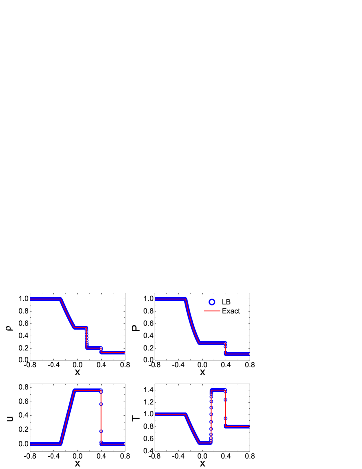
Figure 1: (Color online) Comparisons between LB results and exact ones for the one-dimensional Sod problem, where $t=0.2$.

For the problem considered, the initial condition is described by

$$\left\{\begin{array}[]{l}\left.{(\rho}\text{{, }}{u}\text{{, }}{v}\text{{, }}{T)}\right|_{L}=(1.0\text{, }0.0\text{, }0.0\text{, }1.0)\text{{,} \ \ \ }x\leq 0\text{;}\\ \left.{(\rho}\text{{, }}{u}\text{{, }}{v}\text{{, }}{T)}\right|_{R}=(0.125\text{, }0.0\text{, }0.0\text{, }0.8)\text{, \ }x>0\text{.}\end{array}\right.$$ (56)

Subscript “$L$" and “$R$" indicate macroscopic variables at the left and right sides of the discontinuity. The size of grid is $\Delta x=\Delta y=10^{-3}$, time step and relaxation time are $\Delta t=\tau=10^{-5}$.

The periodic boundary conditions are taken in the $y$ direction. In the $x$ direction, we set

$$f_{ki\text{,}-2\text{,}t}=f_{ki\text{,}-1\text{,}t}=f_{ki\text{,}0\text{,}t}=f_{ki\text{,}1\text{,}t=0}^{(0)}\text{,}$$ (57)

where $-2$, $-1$ and $0$ are the indexes of ghost nodes on the left side. Such a boundary condition means that the system at the boundaries keeps at their corresponding equilibrium states and the macroscopic quantities on the boundary nodes keep their initial values QuKun ; HYL ,

$$(\rho\text{, }u\text{, }v\text{, }P)_{I=-2\text{,}t}=(\rho\text{, }u\text{, }v\text{, }P)_{I=-1\text{,}t}=(\rho\text{, }u\text{, }v\text{, }P)_{I=0\text{,}t}=(\rho\text{, }u\text{, }v\text{, }P)_{I=1\text{,}t=0}\text{.}$$ (58)

On the right boundary, we can do in a similar way. The boundary conditions in the $x$-direction are also referred to as the supersonic inflow boundary conditions QuKun . Eq.(57) and Eq.(58) may be referred to as the microscopic and the macroscopic boundary conditions, respectively, which are consistent with each other.

It is worth noting that when the external environment is in equilibrium the boundary conditions for the FDLB model are essentially the same as those in traditional computational fluid dynamics (CFD). When the external environment is not in equilibrium, the non-equilibrium part $f_{ki\text{,}I}^{(neq)}$ can be obtained from the inner lattice nodes via the extrapolation method. That nonequilibrium effects can be incorporated from boundary conditions is a merit of LB method over the traditional CFD.

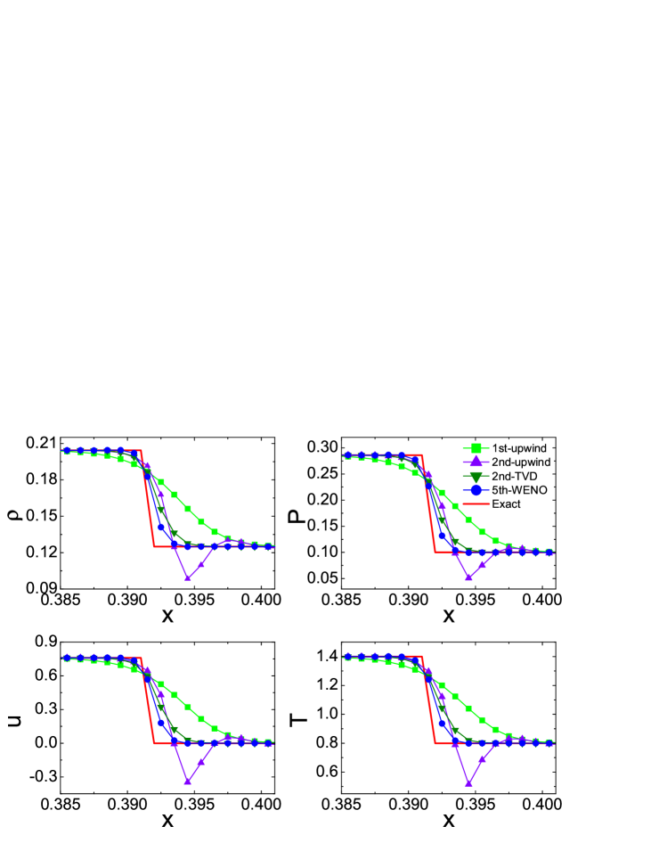
Figure 2: (Color online) Local details of the profiles near the shock wave for Sod shock problem at $t=0.2$. The 1st-upwind scheme, the 2nd-upwind scheme, the 2nd-TVD scheme, and the 5th-WENO scheme are adopted in spatial discretization for comparisons.

Figure 1 shows the computed density, pressure, velocity, and temperature profiles at $t=0.2$, where the circles are for simulation results and solid lines are for analytical solutions. The two sets of results have a satisfying agreement. Figure 2 enlarges the part containing the shock wave for a closing view. The first-order upwind (1st-upwind) scheme, the second order upwind (2nd-upwind) scheme, the second order total variation diminishing (2nd-TVD) scheme NND , and the 5th-WENO scheme are adopted in spatial discretization for comparisons. One can see that the 1st-upwind scheme has a strong “smoothing effect" and gives a very smeared solution with excessive numerical dissipation. Compared to the former, the 2nd-upwind scheme has a weak “smoothing effect", but it introduces the unphysical oscillations at discontinuities. The 2nd-TVD scheme effectively eliminates the spurious numerical oscillations at discontinuities, while the numerical dissipation may need to be reduced further. However, with the 5th-WENO scheme, not only the spurious numerical oscillations at discontinuities are effectively refrained but also the numerical dissipation is severely curtailed. With an increase in the order of the schemes, fewer nodes are needed to capture the shock waves. The widths of the shock waves are spread over only about three to four grid cells with the 5th-WENO scheme, which shows that the LB model with the WENO scheme has a high ability to capture shocks for this test.

IV Effects of velocity and density gradients on KHI

At the initial linear increasing stage of KHI, the amplitude $\eta$ of perturbation evolves according to the following relation, $\eta=\eta_{0}e^{\gamma t}$, where $\gamma$ is the growth coefficient and is dependent on the gradient of tangential velocity and gradient of density around the interface ICF-book . In other words, $\gamma$ is dependent on the width of velocity transition layer $D_{v}$ and width of density transition layer $D_{\rho}$. In this section, we discuss separately the KHI in three cases, (i) $D_{v}$ is variable and $D_{\rho}$ is fixed, (ii) $D_{\rho}$ is variable and $D_{v}$ is fixed, (iii) both $D_{\rho}$ and $D_{v}$ are variable. The increasing rate $\gamma$ for case (i), (ii) and (iii) are referred to as $\gamma_{v}$, $\gamma_{\rho}$ and $\gamma_{R}$, respectively. We numerically obtain $\gamma_{v}$, $\gamma_{\rho}$ and $\gamma_{R}$ via fitting the curves of $\ln E_{x}|_{\max}(t)$ versus the time $t$, where $E_{x}|_{\max}(t)$ is the maximum of $E_{x}(x,y,t)$ in the whole computational domain, $E_{x}(x,y,t)=\rho(x,y,t)u^{2}(x,y,t)/2$ is the perturbed kinetic energy at the position ($x$, $y$) at each time step $t$.

IV.1 Linear growth rate and velocity gradient effect

The initial configurations in our simulation are described by

$$\rho(x)=\frac{{\rho_{L}+\rho_{R}}}{2}-\frac{{\rho_{L}-\rho_{R}}}{2}\tanh(\frac{x}{{D_{\rho}}})\text{,}$$ (59)

$$v(x)=\frac{{v_{L}+v_{R}}}{2}-\frac{{v_{L}-v_{R}}}{2}\tanh(\frac{x}{{D_{v}}})\text{,}$$ (60)

$$P_{L}=P_{R}=P\text{,}$$ (61)

where ${D_{\rho}}$ and ${D_{v}}$ are the widths of density and velocity transition layers. The velocity(density) is discontinuous at $x=0$ when ${D_{v}=0}$(${D_{\rho}=0}$). ${\rho_{L}=5.0}$(${\rho_{R}=2.0}$) is the density away from the interface of the left(right) fluid. ${v_{L}=0.5}$(${v_{R}=-0.5}$) is the velocity away from the interface in $y$-direction of the left(right) fluid and $P_{L}$($P_{R}$)$=2.5$ is the pressure in the left(right) side. The Mach numbers of the left side and the right side of the simulation domain are $0.5$ and $0.32$, respectively. Hence the flow speed $v_{0}$ is subsonic and the system can be approximately thought of as “incompressible". The whole calculation domain is a rectangle with length $0.6$ and height $0.2$, which is divided into $600\times 200$ uniform meshes. A simple velocity perturbation in the $x$-direction is introduced to trigger the KH rollup and it is in the following form

$$u=u_{0}\sin(ky)\exp(-kx)\text{,}$$ (62)

where $u_{0}=0.02$ is the amplitude of the perturbation. Here, $k$ is the wave number of the initial perturbation, and is set to be $10\pi$. The time step is $\Delta t=10^{-5}$. Extensive studies indicate that viscosity will damp the evolution of the KHI. However, for the KHI in some cases, for example, in ICF, effects of the viscosity are generally negligible. Therefore, throughout the simulations, $\tau$ is set to be $10^{-5}$ to reduce the physical viscosity. Boundary conditions for the simulations of KHI are as below. Periodic boundary conditions are used in the $y$-direction. In the horizontal direction, we adopt the outflow (zero gradient) boundary conditions, which are widely used by other authors to simulate the KHI outflow-KHI-1 ; outflow-KHI-2 ; outflow-KHI-3 . For the outflow boundary conditions, the zeroth-order extrapolation is used QuKun . According to this boundary conditions, at the left side, we set

$$(\rho\text{, }u\text{, }v\text{, }P)_{I=-2\text{,}t}=(\rho\text{, }u\text{, }v\text{, }P)_{I=-1\text{,}t}=(\rho\text{, }u\text{, }v\text{, }P)_{I=0\text{,}t}=(\rho\text{, }u\text{, }v\text{, }P)_{I=1\text{,}t}\text{.}$$ (63)

and at the right side

$$(\rho\text{, }u\text{, }v\text{, }P)_{I=N_{x}+3\text{,}t}=(\rho\text{, }u\text{, }v\text{, }P)_{I=N_{x}+2\text{,}t}=(\rho\text{, }u\text{, }v\text{, }P)_{I=N_{x}+1\text{,}t}=(\rho\text{, }u\text{, }v\text{, }P)_{I=N_{x}\text{,}t}\text{,}$$ (64)

where $I=-2$, $-1$, $0$ and $N_{x}+1$, $N_{x}+2$, $N_{x}+3$ are the indexes of left and the right ghost nodes, respectively.

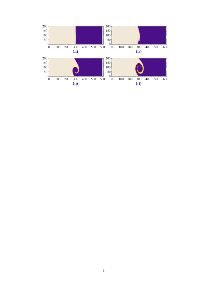
Figure 3: (Color online) Density evolutions of KHI simulated using the LB model, where $D_{v}=4$ and ${D_{\rho}=8}$, $t=0.1$ in (a), $t=0.3$ in (b), $t=0.5$ in (c), and $t=0.7$ in (d).

Figure 3 shows the temporal evolution of the density field for ${D_{v}=4}$ and ${D_{\rho}=8}$ at four different times. It is clear that at $t=0.3$ the interface is wiggling due to the initial perturbation and the velocity shear. After the initial linear growth stage, there is a nicely rolled vortex developing around the initial interface. A larger vortex is observed in the snapshot at $t=0.7$, and a mixing layer is expected to be formed around the initial interface. The interface is continuous and smooth, which indicates the LB model has a good capturing ability of interface deformation.

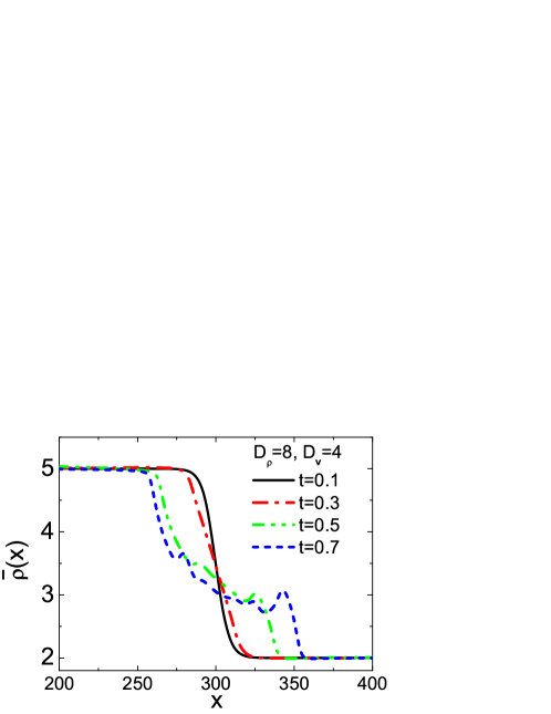
Figure 4: (Color online) Averaged density profiles along the $x$-axis at $t=0.1$ (solid line), $t=0.3$ (dash dot line), $t=0.5$ (dash dot dot line), and $t=0.7$ (short dash line) for ${D_{\rho}=8}$ and ${D_{v}=4}$.

To quantitatively describe the characteristics of the vortex or the mixing layer, in Fig.4 we plot the averaged density profile $\overline{\rho}(x)$ against the $x$-axis at $t=0.1$, $0.3$, $0.5$ and $0.7$. The averaged density in the mixing layer is defined as

$$\overline{\rho}(x)=\frac{1}{L}\int_{0}^{L}{\rho(x,y)dy}\text{.}$$ (65)

The averaged density profiles vary from being smooth to being irregular. The thickness of the mixing layer and the amplitude of the density oscillation increase with time. The zig-zags in the profiles indicate the transfer of fluids from the dense to the rarefactive regions and the irregularity in the mixing layer.

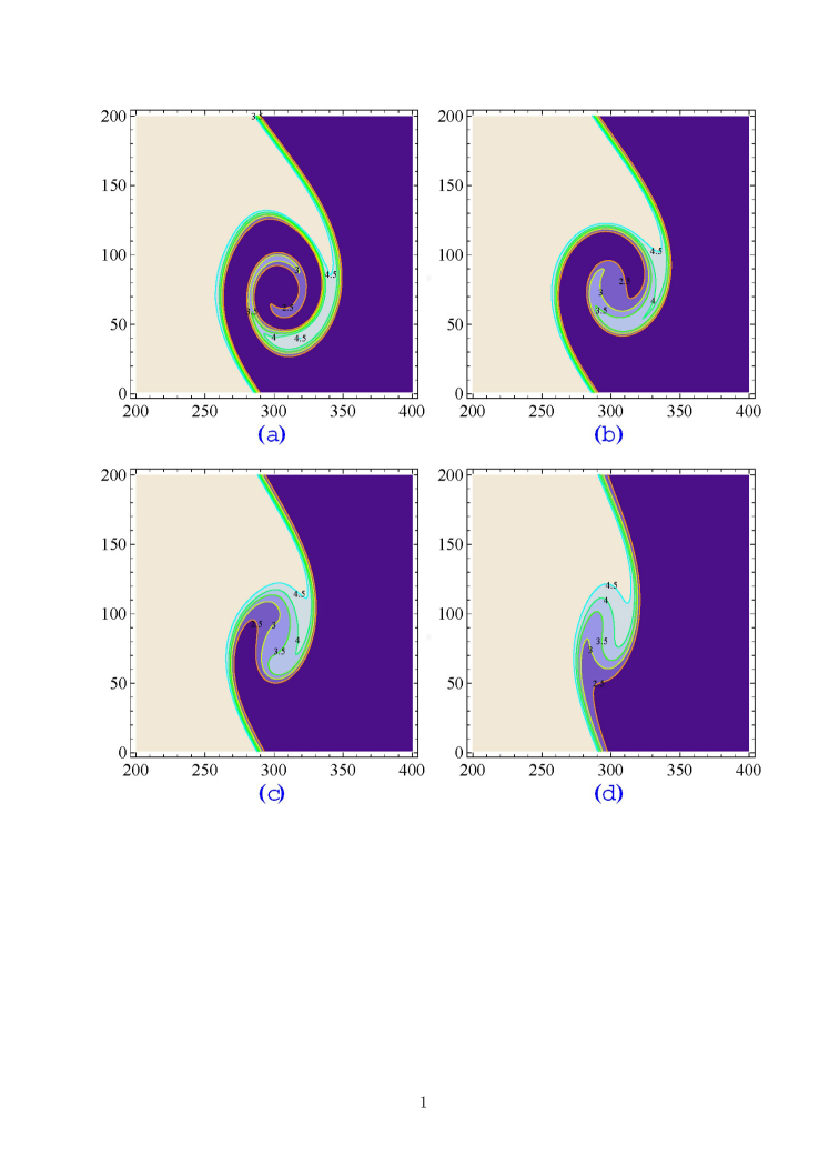
Figure 5: (Color online) Vortices in the mixing layer as a function of ${D_{v}}$ at $t=0.6$, where ${D_{v}=4}$ in (a), ${D_{v}=8}$ in (b), ${D_{v}=12}$ in (c), and ${D_{v}=16}$ in (d). The density transition layer ${D_{\rho}}$ is fixed to be $8$.

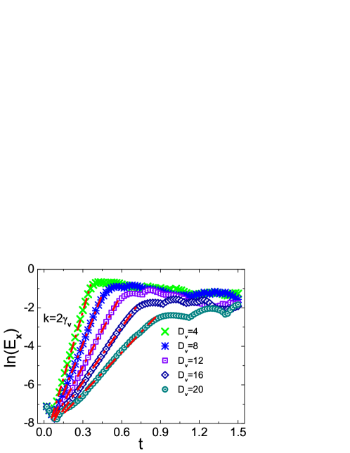
Figure 6: (Color online) Time evolution of the perturbed peak kinetic energy $E_{x}|_{\max}$ along the $x$-axis in $\ln$-linear scale for various widths of velocity transition layer. The dash-dotted lines represent the linear fits to the initial linear growth regimes.

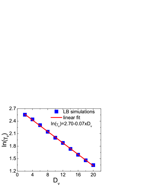
Figure 7: (Color online) Linear growth rate as a function of the width ${D_{v}}$ of velocity transition layer.

To consider the velocity gradient effect, the simulations with various ${D_{v}}$ have been performed and the density maps for ${D_{v}=4}$, ${8}$, ${12}$, and $16$ with five contour lines at $t=0.6$ are plotted in Fig.5. We see that the width of the velocity transition layer can significantly affect the evolution of KHI. For fixed density gradient and velocity difference, the larger the value of $D_{v}$, i.e., the wider the initial transition zone, the weaker the KHI, and the later the vortex appears. In Fig.5(a) and Fig.5(b), the appearance of large vortices demonstrates that the evolution is embarking on the nonlinear stage. While in Fig.5(c) and Fig.5(d), the width of the mixing layers is rapidly decreased by the increase of ${D_{v}}$ and the evolution is in the weakly nonlinear stage. Figures 5(a)-(d) show that a wider velocity transition zone has a better stabilization effect on KHI.

Taking the logarithm of the perturbed peak kinetic energy $E_{x}|_{\max}$ of each time step, the exponential growth manifests itself as a linear slope ek ; ek2 ; ek3 (see Fig.6). Therefore, $\gamma$ can be obtained from the slope of a linear function fitted to the initial growth stage. We note in this respect that $E_{x}\propto$ $u^{2}\propto\left(e^{\gamma t}\right)^{2}$ grows at twice the rate of the KHI, namely $k=2\gamma$, where $k$ is the slope of the linear fit. The peak kinetic energy $E_{x}|_{\max}$ can represent the interacting strength of two different fluids. It is clear from Fig.6 that the logarithm of the perturbed kinetic energy first grows linearly in time and then arrives at a nonlinear saturation procedure at late times.

For a fixed ${D_{v}}$ and ${D_{\rho}}$, $E_{x}|_{\max}$ increases with time $t$ during the linear growth stage. However, at the same time, the larger the value of $D_{v}$, the smaller the perturbed peak kinetic energy $E_{x}|_{\max}$. This means when the transition layer becomes wider, the evolution of the density field becomes slower. Moreover, we find that the dependence of $\gamma_{v}$ on $D_{v}$ can be fitted by a logarithmic function with the form

$$\ln\gamma_{v}=a-bD_{v}\text{,}$$ (66)

with $a=2.70$ and $b=0.07$ as displayed in Fig.7. The numerical simulation result is in general agreement with the analytical results (see Eq.(18) and Fig.3 in recent work of Wang, et al. wang-pop-2010 ). In the classical case, the linear growth rate is $\gamma_{c}=k\sqrt{\rho_{1}\rho_{2}}(v_{1}-v_{2})/(\rho_{1}+\rho_{2})\propto\Delta v$, where $\Delta v$ is the shear velocity difference. A wider transition layer decreases the local or the effective shear velocity difference $\Delta{v}$, which results in a smaller linear growth rate, a smaller saturation energy, and a longer linear growth time $t_{lin}$.

IV.2 Linear growth rate and density gradient effect

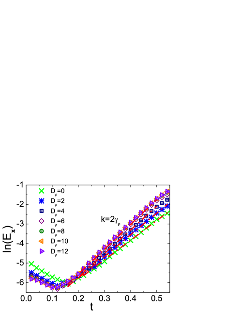
Figure 8: (Color online) Time evolution of the logarithm of the peak kinetic energy $E_{x}|_{\max}$ along the $x$-axis for various widths of density transition layers.

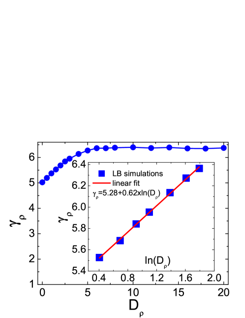
Figure 9: (Color online) Linear growth rate as a function of the width ${D}_{\rho}$ of density transition layer.

In this subsection, the density gradient effect is investigated in a similar way. The initial conditions are described as, $({\rho_{L}}$, ${v_{L}}$, $P_{L})=(5.0$, $0.5$, $1.5)$ and $({\rho_{R}}$, ${v_{R}}$, $P_{R})=(1.25$, $-0.5$, $1.5)$. Parameters are set to be $dx=dy=0.002$, $\Delta t=10^{-5}$. Figure 8 shows time evolution of the logarithm of the peak kinetic energy $E_{x}|_{\max}$ along the $x$-axis with various widths of density transition layers. It is seen in Fig.8, for fixed width $D_{v}$ of velocity transition layer and fixed density difference, the linear growth rate first increases with the width $D_{\rho}$ of density transition layer. But when ${D_{\rho}}>6$, the linear growth rate does not vary significantly any more (see Fig.8 for details), which indicates the effective interaction width of $D_{\rho}$ is less than that of $D_{v}$. Moreover, we find when ${D_{\rho}}<6$, the dependence of $\gamma_{\rho}$ on $D_{\rho}$ can be fitted by the following equation

$$\gamma_{\rho}=c+e\ln D_{\rho}\text{,}$$ (67)

with $c=5.28$ and $e=0.62$ as shown in the legend of Fig.9. The numerical simulation results are also in general agreement with the analytical results (see Fig.2 in previous work by Wang, et al. wang-pop-2009 , Eq.(18) and Fig.2 in recent work of Wang, et al. wang-pop-2010 ). In the classical case, the square of the linear growth rate is $\gamma_{c}^{2}=k^{2}\rho_{1}\rho_{2}(v_{1}-v_{2})^{2}/(\rho_{1}+\rho_{2})^{2}\propto(1-A^{2})\Delta v^{2}$, where $A=(\rho_{1}-\rho_{2})/(\rho_{1}+\rho_{2})$ is the Atwood number. A wider density transition zone reduces the Atwood number around the interface. Then in the process of exchanging momentum in the direction normal to the interface, the perturbation can obtain more energy from the shear kinetic energy than in cases with sharper interfaces. Therefore, a wider density transition layer increases the linear growth rate of the KHI.

IV.3 Hybrid effects of velocity and density gradients

In practical systems, at the interface of two fluids with a tangential velocity difference, both the velocity and the density gradients exist. The wider velocity transition layer decreases the linear growth rate of the KHI, but the wider density transition layer strengthens it. Consequently, there is a competition between these two gradient effects. In this section, we investigate how these two effects compete with each other. For convenience, we introduce a coefficient $R=D_{\rho}/D_{v}$ to analyze the combined effect. The linear growth rate at various velocity and density gradients for $R=0.5$, $1$, $2$, and $5$ are illustrated in Fig.10.

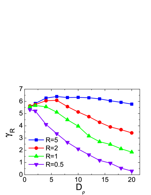
Figure 10: (Color online) The linear growth rate versus the width of density transition layer for $R=0.5$, $1$, $2$, and $5$. The initial density, shear velocity and pressure of the two fluids are $({\rho_{L}}$, ${v_{L}}$, $P_{L})=(5.0$, $0.5$, $1.5)$ and $({\rho_{R}}$, ${v_{R}}$, $P_{R})=(1.25$, $-0.5$, $1.5).$

As shown in Fig.10, on the whole, the hybrid effect of velocity and density transition layers reduces the linear growth rate $\gamma_{R}$. Only at small $D_{\rho}$ and when $R>1$, the hybrid effect of velocity and density transition layers makes larger the linear growth rate. This indicates that the effective interaction width of the velocity transition layer ${D_{v}^{E}}$ is wider than that of density transition layer ${D_{\rho}^{E}}$.

For a fixed value of $R$ ($>1$), when $D_{\rho}$ is small, the transfer efficiency of kinetic energy between neighboring layers increases with decreasing the density gradient, so the linear growth rate increases with $D_{\rho}$ and reaches a peak. When $D_{\rho}$ is greater than the peak value, the stabilizing effect of velocity transition layer becomes more significant and stronger than the destabilizing effect of the density transition layer, which leads to the decreasing of linear growth rate with $D_{\rho}$, as shown in Fig.10 of $R=1$, $2$, and $5$ cases. However, when $R<1$, the linear growth rate decreases monotonically with $D_{\rho}$, no matter it is small or large.

V Conclusions and discussions

In this paper, a two-dimensional LB model with 19 discrete velocities in six directions is proposed. The model allows to recover the compressible Euler equations in the continuum limit. With the introduction of the 5th-WENO FD scheme, the unphysical oscillations at discontinuities are effectively suppressed and the numerical dissipation is severely curtailed. The validity of the model is verified by its application to the Sod shock tube, and excellent agreement between the simulation results and the analytical solutions can be found.

Using the proposed LB model, the velocity and density gradient effects on the KHI have been studied. The averaged density profiles, and the peak kinetic energy are used to quantitatively describe the evolution of KHI. It is found that evolution of the KHI is damped with increasing the width of velocity transition layer but is strengthened with increasing the width of density transition layer. After the initial transient period and before the vortex has been well formed, the linear growth rates, $\gamma_{v}$ and $\gamma_{\rho}$, vary with ${D_{v}}$ and ${D_{\rho}}$ approximately in the following way, $\ln\gamma_{v}=a-bD_{v}$ and $\gamma_{\rho}=c+e\ln D_{\rho}({D_{\rho}}<{D_{\rho}^{E}})$, where $a$, $b$, $c$ and $e$ are fitting parameters and ${D_{\rho}^{E}}$ is the effective interaction width of density transition layer. When ${D_{\rho}}>{D_{\rho}^{E}}$ the growth rate $\gamma_{\rho}$ goes to nearly a constant and the destabilizing effect of density gradient on KHI is fixed. These can be understood as follows. As noted above, in the classical case, the square of the linear growth rate is $\gamma_{c}^{2}=k^{2}\rho_{1}\rho_{2}(v_{1}-v_{2})^{2}/(\rho_{1}+\rho_{2})^{2}\propto(1-A^{2})\Delta v^{2}$. The wider velocity transition layer reduces the the local velocity difference $\Delta v$ and the wider density transition zone reduces the local Atwood number $A$. Therefore, the linear growth rate can be decreased by ${D_{v}}$ but made larger by $D_{\rho}$. In practical system, both the two transition layers exist and there is a competition between these two gradient effects. One can use the hybrid effects of density and velocity transition layers to stabilize the KHI. By incorporating an appropriate equation of state, or equivalently, a free energy functional, or an external force, the present model may be used to simulate the liquid-vapor transition and the surface tension effects on KHI.

References

- (1) S. Succi, The Lattice Boltzmann Equation for Fluid Dynamics and Beyond, (Oxford University Press, New York, 2001).
- (2) M. R. Swift, W. R. Osborn, and J. M. Yeomans, Phys. Rev. Lett. 75, 830 (1995); G. Gonnella, E. Orlandini, and J. M. Yeomans, Phys. Rev. Lett. 78, 1695 (1997); A. J. Wagner and J. M. Yeomans, Rev. Lett. 80, 1429 (1998); D. Marenduzzo, E. Orlandini, and J. M. Yeomans, Phys. Rev. Lett. 92, 188301 (2004).
- (3) Aiguo Xu, G. Gonnella, and A. Lamura, Phys. Rev. E 67, 056105 (2003); Phys. Rev. E 74, 011505 (2006); Physica A 331, 10 (2004); Physica A 344, 750 (2004); Physica A 362, 42 (2006); Aiguo Xu, G. Gonnella, A. Lamura, G. Amati, and F. Massaioli, Europhys. Lett. 71, 651 (2005).
- (4) V. Sofonea and K. Mecke, Eur. Phys. J. B 8, 99 (1999); V. Sofonea, A. Lamura, G. Gonnella, and A. Cristea, Phys. Rev. E 70, 046702 (2004); G. Gonnella, A. Lamura, and V. Sofonea, Phys. Rev. E 76, 036703 (2007); A. Cristea, G. Gonnella, A. Lamura, and V. Sofonea, Commun. Comput. Phys. 7, 350 (2010).
- (5) S. Y. Chen, H. D. Chen, D. Martinez, and W. Matthaeus, Phys. Rev. Lett. 67, 3776 (1991).
- (6) S. Succi, M. Vergassola and R. Benzi, Phys. Rev. A 43, 4521 (1991).
- (7) G. Vahala, B. Keating, M. Soe, J. Yepez, L. Vahala, J. Carter, and S. Ziegeler, Comm. Comp. Phys. 4, 624 (2008).
- (8) J. Yepez, Int. J. Mod. Phys. C 12, 1285 (2001).
- (9) G. P. Berman, A. A. Ezhov, D. I. Kamenev, and J. Yepez, Phys. Rev. A 66, 012310 (2002).
- (10) K. Furtado and J. M. Yeomans, Phys. Rev. E 73, 066124 (2006).
- (11) C. H. Sun, Phys. Rev. E 58, 7283 (1998).
- (12) T. Kataoka and M. Tsutahara, Phys. Rev. E 69, 035701(R) (2004); Phys. Rev. E 69, 056702 (2004).
- (13) M. Watari and M. Tsutahara, Phys. Rev. E 67, 036306 (2003); Phys. Rev. E 70, 016703 (2004).
- (14) Aiguo Xu, Europhys. Lett. 69, 214 (2005); Phys. Rev. E 71, 066706 (2005); Prog. Theor. Phys. (Suppl.) 162, 197 (2006).
- (15) Yanbiao Gan, Aiguo Xu, Guangcai Zhang, Xijun Yu, and Yingjun Li, Physica A 387, 1721 (2008).
- (16) Feng Chen, Aiguo Xu, Guangcai Zhang, Yingjun Li, and Sauro Succi, Europhys. Lett. 90, 54003 (2010).
- (17) K. Qu, C. Shu, and Y. T. Chew, Phys. Rev. E 75, 036706 (2007).
- (18) Q. Li, Y. L. He, Y. Wang, and W. Q. Tao, Phys. Rev. E 76, 056705 (2007); Q. Li, Y. L. He, Y. Wang, and G. H. Tang, Phys. Lett. A 373, 2101 (2009); Y. Wang, Y. L. He, T. S. Zhao, G. H. Tang, and W. Q. Tao, Int. J. Mod. Phys. C 18, 1961 (2007).
- (19) J. Y. Zhang and G. W. Yan, Phys. Rev. E 81, 066705 (2010); Chaos 20, 023129 (2010).
- (20) Q. F. Wu and W. F. Chen, DSMC method for heat chemical nonequilibrium flow of high temperature rarefied gas, (National Defence Science and Technology University Press, Beijing, 1999), (in Chinese).
- (21) S. Chandrasekhar, Hydrodynamic and Hydromagnetic Stability, (Oxford University, London, 1961).
- (22) J. S. Walker, G. Talmage, S. H. Brown, and N. A. Sondergaard, Phys. Fluids A 5, 1466 (1993).
- (23) H. H. Bau, Phys. Fluids 25, 1719 (1982).
- (24) J. W. Miles, Phys. Fluids 23, 1719 (1980).
- (25) L. F. Wang, C. Xue, W. H. Ye, and Y. J. Li, Phys. Plasma 16, 112104 (2009).
- (26) L. F. Wang, W. H. Ye, and Y. J. Li, Phys. Plasma 17, 042103 (2010).
- (27) A. Miura, Phys. Rev. Lett. 83, 1586 (1999).
- (28) R. Blaauwgeers, V. B. Eltsov, G. Eska, A. P. Finne, R. P. Haley, M. Krusius, J. J. Ruohio, L. Skrbek, and G. E. Volovik, Phys. Rev. Lett. 89, 155301 (2002).
- (29) G. Bodo, A. Mignone, and R. Rosner, Phys. Rev. E 70, 36304 (2004).
- (30) W. Horton, J. C. Perez, T. Carter, and R. Bengtson, Phys. Plasmas 12, 22303 (2005).
- (31) L. F. Wang, W. H. Ye, Z. F. Fan, Y. J. Li, X. T. He, and M. Y. Yu, Europhys. Lett. 86, 15002 (2009).
- (32) R. P. Drake, High-Energy-Density Physics: Fundamentals, Inertial Fusion and Experimental Astrophysics, (Springer, New York, 2006).
- (33) M. Lesieur, Turbulence in Fluids, (Kluwer Academic Publishers, Dordrecht, 1997).
- (34) V. N. Gamexo, A. M. Khokhlo, E. S. Oran, A. Y. Chtchelkanova, and R. O. Rosenberg, Science 299, 77 (2003).
- (35) A. Burrows, Nature (London) 430, 727 (2000).
- (36) K. Nomoto, K. Iwamoto, and N. Kishimoto, Science 276, 1378 (1997).
- (37) H. Hasegawa, M. Fujimoto, T. D. Phan, H. R me, A. Balogh, M. W. Dunlop, C. Hashimoto, and R. TanDokoro, Nature (London) 430, 755 (2004).
- (38) L. F. Wang, W. H. Ye, and Y. J. Li, Phys. Plasma 17, 052305 (2010).
- (39) L. F. Wang, W. H. Ye, Z. F. Fan, and Y. J. Li, Europhys. Lett. 90, 15001 (2010).
- (40) B. A. Remington, R. P. Drake, H. Takabe, and D. Arnett, Phys. Plasmas 7, 1641 (2000).
- (41) B. A. Remington, R. P. Drake, and D. D. Ryutov, Rev. Mod. Phys. 78 755 (2006).
- (42) S. Atzeni and J. Merer-ter-Vehn, The Physics of Inertial Fusion, (Oxford University Press, New York, 2004).
- (43) G. Chimonas, Phys. Fluids 29, 2061 (1986).
- (44) G. S. Jiang and C. W. Shu, J. Comput. Phys. 126, 202 (1996).
- (45) C. W. Shu and S. Osher, J. Comput. Phys. 77, 439 (1988).
- (46) X. D. Liu, S. Osher, and T. Chan, J. Comput. Phys. 115, 200 (1994).
- (47) G. A. Sod, J. Comput. Phys. 27, 1 (1978).
- (48) H. X. Zhang, Acta Aerodyn. Sin. 6, 143 (1988).
- (49) R. Keppens and G. T ah, Phys. Plasma 6, 1461 (1999).
- (50) M. Perucho, M. Hanasz, J. M. Marti, and J. A. Miralles, Phys. Rev. E 75, 056312 (2007).
- (51) L. F. Wang, A. P. Teng, W. H. Ye, C. Xue, Z. F. Fan, and Y. J. Li, Commun. Theor. Phys. 52, 694, 056312 (2009).
- (52) U. V. Amerstorfer, N. V. Erkaev, U. Taubenschuss, and H. K. Biernat, Phys. Plasma 17, 072901 (2010).
- (53) Ashwin J. and R. Ganesh, Phys. Rev. Lett. 104, 215003 (2010).
- (54) M. Obergaulinger, M. A. Aloy, and E. Müller, A&A 515, A30 (2010).