Order thresholding

Abstract

A new thresholding method, based on L-statistics and called order thresholding, is proposed as a technique for improving the power when testing against high-dimensional alternatives. The new method allows great flexibility in the choice of the threshold parameter. This results in improved power over the soft and hard thresholding methods. Moreover, order thresholding is not restricted to the normal distribution. An extension of the basic order threshold statistic to high-dimensional ANOVA is presented. The performance of the basic order threshold statistic and its extension is evaluated with extensive simulations.

T1Supported in part by NSF Grants SES-0318200 and DMS-08-05598.

and

1 Introduction

It is well known that, when testing against a high-dimensional alternative, omnibus tests designed to detect any departure from the null hypothesis have low power. Neyman’s (1937) truncation idea, though motivated by a different type of problem, served as the spring board for the development of modern related approaches. Soft and hard thresholding were introduced in the context of nonparametric function estimation using wavelets by Donoho and Johnstone (1994). Johnstone and Silverman (2004) elaborate on a number of additional applications of thresholding including image processing, model selection, and data mining. Beran (2004) considered applications to the one-way ANOVA design. Spokoiny (1996), Fan (1996) and Fan and Lin (1998) consider applications of thresholding methods to testing problems. Fan (1996) found that hard thresholding outperforms both soft thresholding and adaptive Neyman’s truncation.

This paper proposes a new thresholding method based on $L$-statistics, which is termed order thresholding. Order thresholding allows great flexibility in the choice of the threshold parameter, can be used for distributions other than the normal, and extends naturally to factorial design settings.

In the simple context where the $X_{i}$ are independent $N(\theta_{i},1)$, $i=1,\ldots,n$, and we wish to test $H_{0}\dvtx\theta_{1}=\cdots=\theta_{n}=0$ vs. $H_{a}\dvtx\theta_{i}\neq 0$, for some $i$, the hard thresholding and order thresholding test statistics are, respectively,

$$T_{H}(\delta_{n})=\sum_{i=1}^{n}Y_{i}I\{Y_{i}>\delta_{n}\}\quad\mbox{and}\quad T_{L}(k_{n})=\sum_{i=1}^{n}c_{in}Y_{i,n},$$ (1)

where $Y_{i}=X_{i}^{2}$, $Y_{1,n}<\cdots<Y_{n,n}$ are the ordered $Y_{i}$’s, $c_{in}=I(i>n-k_{n})$, and $\delta_{n}$, $k_{n}$ are the corresponding threshold parameters. Thus, $T_{L}(k_{n})$ is an $L$-statistic based on the largest $k_{n}$ squared observations. Conceptually, the connection between hard thresholding and order thresholding is similar to that between type I and type II censoring. The main difference being that the threshold parameters in type I and type II censoring (the cut-off point and the proportion of observations included, resp.) remain fixed, while in the present case they change with the sample size. As we will see, this distinction implies very different asymptotic behavior.

The idea behind both statistics in (1) is similar to that of Neyman’s truncation. Namely, when the “signal” is known to be concentrated in a few locations, the accumulation of stochastic errors has a negative impact on the performance of the procedure based on the chi-square statistic

$$T_{L}(n)=\sum_{i=1}^{n}Y_{i}.$$ (2)

Since the signal locations are not known, the statistics in (1) attempt to minimize the accumulation of noise by focusing on the observations with the largest absolute values. The asymptotic theory for hard thresholding [Fan (1996)] requires several restrictive conditions that prevent its general applicability. For example, the centering and scaling of $T_{H}(\delta_{n})$ in (1) are specific to the normality assumption and to the choice of $\delta_{n}$. Moreover, $\delta_{n}$ is required to tend to infinity at a rate that is specific to the normality assumption. For example, $\delta_{n}$ tending to infinity is clearly not appropriate if the $X_{i}$ have bounded support. (Below, we discuss an application to multiple testing where the $X_{i}$ are uniformly distributed.) Intuitively, if the signal is present in more locations, it is advantageous to lower the value of the hard threshold parameter. The advantage of allowing different values of the threshold parameter is amply illustrated in Johnstone and Silverman (2004). However, the asymptotic theory of $T_{H}(\delta_{n})$ requires the threshold parameter to tend to infinity at specific rates. In particular, it must be of the form $\delta_{n}=2\log(na_{n})$, where $a_{n}=c(\log n)^{-d}$, for $c>0$ and $d>0.5$. Thus, if we let $k_{H}(\delta_{n})$ denote the random number of observations considered in $T_{H}(\delta_{n})$, the asymptotic theory of $T_{H}(\delta_{n})$ requires $E[k_{H}(\delta_{n})]$ to converge to infinity at the rate of

$$\frac{(\log n)^{d}}{\sqrt{\log n+d\log(c^{1/d}(\log n)^{-1})}}$$

or, roughly, $(\log n)^{d-0.5}$. In contrast, the asymptotic theory of $T_{L}(k_{n})$ allows the threshold parameter $k_{n}$ to tend to infinity at any rate.

While the asymptotic theory of $T_{H}(\delta_{n})$ allows some flexibility in the choice of $\delta_{n}$, the convergence of the distribution of $T_{H}(\delta_{n})$ to its limiting distribution is very slow unless $c=1$ and $d=2$ [Fan (1996)]. The following tables show that small departures in the recommended value of $d$, while keeping $c=1$, have significant effect on the level of the test. The results are based on 30,000 simulation runs.

Table 1: Type I errors of $T_{H}(\delta_{n})$ for different values of the hard threshold parameter

	$\bolds{\delta_{n}-2.0}$	$\bolds{\delta_{n}-1.6}$	$\bolds{\delta_{n}-1.2}$	$\bolds{\delta_{n}-0.8}$	$\bolds{\delta_{n}-0.4}$	$\bolds{\delta_{n}}$
$n=50$	0.0003	0.0099	0.0231	0.0341	0.0431	0.0493
$n=100$	0.0101	0.0229	0.0324	0.0390	0.0461	0.0504
$n=200$	0.0231	0.0316	0.0382	0.0439	0.0484	0.0507
$n=500$	0.0327	0.0388	0.0422	0.0465	0.0502	0.0535

Table 2: Type I errors of $T_{H}(\delta_{n})$ for different values of the hard threshold parameter

	$\bolds{\delta_{n}+0.4}$	$\bolds{\delta_{n}+0.8}$	$\bolds{\delta_{n}+1.2}$	$\bolds{\delta_{n}+1.6}$	$\bolds{\delta_{n}+2.0}$
$n=50$	0.0543	0.0588	0.0614	0.0654	0.0663
$n=100$	0.0552	0.0559	0.0597	0.0616	0.0631
$n=200$	0.0539	0.0562	0.0590	0.0601	0.0627
$n=500$	0.0540	0.0563	0.0583	0.0604	0.0623

To fully appreciate the results reported in Table 1, we mention that for $n=500$ the recommended $\delta_{500}$ value is 5.1216, while the value $\delta_{500}-2$ corresponds to $c=1$ and $d=2.5474$. We see that even with this small departure from the recommended value, the achieved alpha level is 0.0327 even with $n=500$. To contrast these results with those of Table 3 for $T_{L}(k_{n})$, note that in Table 3 with $n=500$, $k_{n}$ ranges from 2 to 500, while in Table 1 with $n=500$, the $E[k_{H}(\delta_{n}+h)]$ ranges from 38.63 for $h=-2.0$ to 11.81 for $h=0$. Thus, the deterioration of the achieved alpha levels occurs as $E[k_{H}(\delta_{n})]$ increases over a relatively small range (in each case, the variance of $k_{H}(\delta_{n})$ is slightly smaller than its expected value). In Table 2 with $n=500$, the $E[k_{H}(\delta_{n}+h)]$ ranges from 9.39 for $h=0.4$ to 3.80 for $h=2.0$, and for this range of values the type I error rate does not change much. In both tables with $n=500$, the variance of the binomial random variable $k_{H}(\delta_{n}+h)$ is slightly smaller than its expected value because $P(Y_{i}\leq\delta_{n}+h)>0.92$ for $-2.0\leq h\leq 2.0$. Finally, following a remark by the AE, we note that the slightly liberal $\alpha$ levels of the $T_{L}(k_{n})$ statistic can be corrected by the use of a multiple of a $\chi^{2}$ distribution to approximate its finite sample distribution. Thus, using the approximation $T_{L}(k_{n})\stackrel{{\scriptstyle\cdot}}{{\sim}}b\chi^{2}_{\nu}$, where $b$ and $\nu$ are chosen to match the mean and variance of $T_{L}(k_{n})$, results in the type I error rates shown in Table 4.

Table 3: Type I errors of $T_{L}(k_{n})$ for different values of the order threshold parameter

	$\bolds{[\log^{1/2}n]}$	$\bolds{[\log n]}$	$\bolds{[\log^{3/2}n]}$	$\bolds{[n^{1/2}]}$	$\bolds{[n^{2/3}]}$	$\bolds{[n^{3/4}]}$	$\bolds{[n^{7/8}]}$	$\bolds{n}$
$n=50$	0.0696	0.0685	0.0646	0.0646	0.0635	0.0630	0.0623	0.0626
$n=100$	0.0669	0.0640	0.0606	0.0600	0.0591	0.0577	0.0585	0.0589
$n=200$	0.0667	0.0620	0.0603	0.0589	0.0582	0.0583	0.0555	0.0560
$n=500$	0.0665	0.0631	0.0577	0.0559	0.0536	0.0536	0.0535	0.0547

Table 4: Type I error rates using the approximation $T_{L}(k_{n})\stackrel{{\scriptstyle\cdot}}{{\sim}}b\chi^{2}_{\nu}$

	$\bolds{[\log^{1/2}n]}$	$\bolds{[\log n]}$	$\bolds{[\log^{3/2}n]}$	$\bolds{[n^{1/2}]}$	$\bolds{[n^{2/3}]}$	$\bolds{[n^{3/4}]}$	$\bolds{[n^{7/8}]}$	$\bolds{n}$
$n=50$	0.0565	0.0545	0.0531	0.0531	0.0532	0.0534	0.0540	0.0546
$n=100$	0.0566	0.0540	0.0520	0.0522	0.0519	0.0507	0.0518	0.0520
$n=200$	0.0555	0.0547	0.0536	0.0531	0.0526	0.0523	0.0530	0.0516
$n=500$	0.0589	0.0556	0.0552	0.0530	0.0520	0.0521	0.0508	0.0505

The greater flexibility in the choice of the threshold parameter that the order threshold statistic offers does not come at the expense of the rate with which it converges to its asymptotic distribution. To emphasize this aspect, Figure 1 presents the estimated densities of the hard thresholding (solid lines in the upper panel) and order thresholding test statistics (solid lines in the lower panel), based on 20,000 simulated values of each statistic using $n=200$. The threshold parameters of the hard thresholding and order thresholding test statistics have been chosen so that the average number of observations included in the two statistics are the same in each column. We see that the estimated densities of the order threshold statistic are closer to the standard normal density (dash-dot line) than those of the hard threshold statistic. In particular, the estimated densities in the upper panel show the rapid deterioration of the quality of the normal approximation to the distribution of $T_{H}(\delta_{200})$ as $\delta_{200}$ shifts away from recommended value of $\delta_{200}=2\log(200\log^{-2}200)=3.9271$.

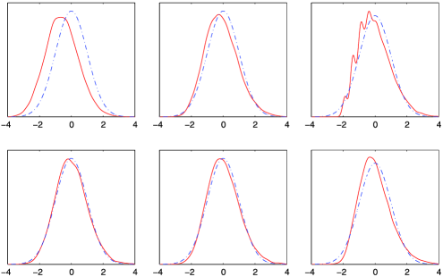
Figure 1: Top panel: estimated densities of $T_{H}(\delta_{200})$ for $\delta_{200}=1.842$, 3.927 and 5.672. Bottom panel: estimated densities of $T_{L}(k_{200})$ for $k_{200}=35$, 10 and 3.

The remaining sections of this paper are organized as follows. In Section 2, we represent a special form of the order statistics using data from an exponential distribution and briefly review the methodology of Chernoff, Gastwirth and Johns (1967). Section 3 develops the order threshold procedure for testing normal means in settings where the number of parameters increases with the sample size, presents simulation results comparing the hard thresholding, a power-enhanced version of the Simes (1986), and order thresholding test statistics, and gives a recommendation for choosing the data-driven value of the threshold parameter. Section 4 extends the order thresholding test procedure to the high-dimensional ANOVA setting [called HANOVA in Fan and Lin (1998)], presents simulation results comparing the power of the classical $F$ and order threshold statistics, and gives a recommendation for a data-driven choice of the order threshold parameter. A discussion summarizing the developments is given in Section 5. Finally, the condensed proofs are given in the Appendix. For detailed proofs, see the archived supplemental material in Kim and Akritas (2010). This is part of the Ph.D. dissertation of the first author.

2 From order statistics to order thresholding: An overview

In the late 1960s when the asymptotic theory of linear combinations of order statistics ($L$-statistics) was developed [cf. Bickel (1967), Chernoff, Gastwirth and Johns (1967), Shorack (1969), Stigler (1969)] the main emphasis was in the estimation of the location parameter. Therefore, the conditions in these papers do not yield automatically the asymptotic distribution of $L$-statistics that assign positive weight to only the largest order statistics. Such $L$-statistics were considered by Nagaraja (1982) in his study of the selection differential for applications to outlier detection. Using results from Hall (1978) and Stigler (1973), he obtained the asymptotic distribution in the extreme and quantile cases, respectively. Here, we will use the conditions from the paper of Chernoff, Gastwirth and Johns (1967), CGJ1967 from now on. Their approach is based on a special representation of the order statistics from the exponential distribution, which we now review.

Let $V_{1},\ldots,V_{n}$ be i.i.d. from the standard exponential distribution, let $V_{1,n}<\cdots<V_{n,n}$ be the corresponding order statistics, and consider the order threshold statistic

$$T_{E,L}(k_{n})=\sum_{i=1}^{n}c_{in}V_{i,n}=\sum_{i=n-k_{n}+1}^{n}V_{i,n}.$$ (3)

The method of CGJ1967 for establishing the asymptotic distribution of $T_{E,L}(k_{n})$ rests on the following well-known property [cf. David and Nagaraja (2003), pages 17 and 18].

Lemma 2.1

The vector of order statistics $(V_{1,n},\ldots,V_{n,n})$ may be represented in distribution by

$$(V_{1,n},\ldots,V_{n,n})\stackrel{{\scriptstyle d}}{{=}}(Y_{1},\ldots,Y_{n}),$$

where

$$Y_{i}=\frac{V_{1}}{n}+\frac{V_{2}}{n-1}+\cdots+\frac{V_{i}}{n-i+1}=\sum_{j=1}^{i}\frac{V_{j}}{n-j+1}.$$

Thus, with $T_{E,L}(k_{n})$ given by (3), it can be represented in distribution as

$$T_{E,L}(k_{n})\stackrel{{\scriptstyle d}}{{=}}\sum_{j=1}^{n}\alpha_{E,jn}(k_{n})V_{j},$$ (4)

where $\alpha_{E,jn}(k_{n})=k_{n}/(n-j+1)$ for $j\leq n-k_{n}$ and $\alpha_{E,jn}(k_{n})=1$ for $j>n-k_{n}$.

Relation (4) expresses $T_{E,L}(k_{n})$ as a linear combination of the independent random variables $V_{1},\ldots,V_{n}$ which enables the use of standard asymptotic results for establishing conditions for its asymptotic distribution. This is given, without proof, in the following.

Theorem 2.1

Let $k_{n},n\geq 1$, be any sequence of integers which satisfies $k_{n}\to\infty$, as $n\to\infty$, and $k_{n}\leq n$, and let $T_{E,L}(k_{n})$ be given in (3). Then we have

$$\quad T_{E,L}^{*}(k_{n})=\frac{T_{E,L}(k_{n})-\sum_{i=1}^{n}\alpha_{E,in}(k_{n})}{\sqrt{\sum_{i=1}^{n}\alpha_{E,in}(k_{n})^{2}}}\stackrel{{\scriptstyle d}}{{\rightarrow}}N(0,1)\qquad\mbox{as }n\to\infty.$$ (5)

In the case where the observations $Y_{i}$, $i=1,\ldots,n$, come from a distribution function $F$, the CGJ1967 approach for obtaining the asymptotic distribution of the order threshold statistic

$$T_{F,L}(k_{n})=\sum_{i=1}^{n}c_{in}Y_{i,n}=\sum_{i=n-k_{n}+1}^{n}Y_{i,n},$$ (6)

where $Y_{1,n}<\cdots<Y_{n,n}$ are the ordered $Y_{i}$’s, is based on the expression $Y_{i,n}=\tilde{H}_{F}(V_{i,n})$, where $\tilde{H}_{F}=F^{-1}\circ G$, and $G$ is the standard exponential distribution function, and the use of Taylor expansion to obtain:

Lemma 2.2 ([Chernoff, Gastwirth and Johns (1967)])

Let $T_{F,L}(k_{n})$ be given by (6). Then,

$$n^{-1}T_{F,L}(k_{n})\stackrel{{\scriptstyle d}}{{=}}\mu_{F,n}(k_{n})+Q_{F,n}(k_{n})+R_{F,n}(k_{n}),$$

where

$$\mu_{F,n}(k_{n}) = \frac{1}{n}\sum_{i=1}^{n}c_{in}\tilde{H}_{F}(\tilde{\nu}_{in}),$$

$$Q_{F,n}(k_{n}) = \frac{1}{n}\sum_{i=1}^{n}\alpha_{F,in}(k_{n})(V_{i}-1)$$

and

$$R_{F,n}(k_{n})=\frac{1}{n}\sum_{i=1}^{n}c_{in}\bigl{\{}\bigl{(}\tilde{H}_{F}(V_{i,n})-\tilde{H}_{F}(\tilde{\nu}_{in})\bigr{)}-(V_{i,n}-\tilde{\nu}_{in})\tilde{H}_{F}^{\prime}(\tilde{\nu}_{in})\bigr{\}}$$

with $\alpha_{F,in}(k_{n})=\frac{1}{n-i+1}\sum_{j=i}^{n}c_{jn}\tilde{H}_{F}^{\prime}(\tilde{\nu}_{jn})$ and $\tilde{\nu}_{in}=\sum_{j=1}^{i}\frac{1}{n-j+1}$.

They then provide conditions under which $Q_{F,n}(k_{n})$ is asymptotically normally distributed and the remainder term, $R_{F,n}(k_{n})$, tends to zero in probability.

3 Single sequence of $N(0,1)$ random variables

In this section, we will apply the approach of CGJ1967 to develop order threshold test procedures for testing the simple hypothesis

$$H_{0}\dvtx\theta_{i}=0\qquad\forall i\quad\mbox{versus}\quad H_{a}\dvtx\mbox{$H_{0}$ is false}$$ (7)

based on a sequence of observations $X_{i},i=1,\ldots,n$, where $X_{i}\sim N(\theta_{i},1)$. The asymptotic null distribution of the order threshold statistic given by (1) is derived in the next subsection, while simulation results comparing the power of the hard threshold statistic, a power-enhanced version of the Simes (1986) statistic, and that of order threshold statistics are presented in Section 3.2. The simulation results suggest that choosing the order threshold parameter equal to the number of the false null hypotheses maximizes the power. Section 3.3 presents a recommendation for a data-driven choice of the order threshold parameter using the idea of Storey (2002, 2003).

3.1 The asymptotic null distribution

Let $X_{i},i=1,\ldots,n$, be standard normal random variables, and let

$$T_{L}(k_{n})=\sum_{i=1}^{n}c_{in}Y_{i,n}=\sum_{i=n-k_{n}+1}^{n}Y_{i,n},$$ (8)

where $Y_{i}=X_{i}^{2}$, $Y_{1,n}<\cdots<Y_{n,n}$ are the ordered $Y_{i}$’s, $c_{in}=I(i>n-k_{n})$, and $k_{n}$ is the order threshold parameter. The approach of CGJ1967 is based on the representation

$$T_{L}(k_{n})\stackrel{{\scriptstyle d}}{{=}}\sum_{i=n-k_{n}+1}^{n}\tilde{H}(V_{i,n}),$$

where $V_{i,n}$, $i=1,\ldots,n$, are the ordered observations from an i.i.d. sequence of $\operatorname{Exp}(1)$ random variables, and

$$\tilde{H}(v)=F^{-1}\circ G(v)$$

with $F(y)=\frac{1}{\sqrt{2\pi}}{\int_{0}^{y}}t^{-1/2}e^{-t/2}\,dt,y>0$, and $G(v)=1-e^{-v}$, $v\geq 0$. Let

$$\mu_{n}(k_{n})=\frac{1}{n}\sum_{i=1}^{n}c_{in}\tilde{H}(\tilde{\nu}_{in}),\qquad\sigma_{n}^{2}(k_{n})=\frac{1}{n}\sum_{i=1}^{n}\alpha_{in}^{2}(k_{n}),$$ (9)

where

$$\alpha_{in}(k_{n}) = \frac{1}{n-i+1}\sum_{j=i}^{n}c_{jn}\tilde{H}^{\prime}(\tilde{\nu}_{jn}),$$

$$\tilde{\nu}_{in} = \sum_{j=1}^{i}\frac{1}{n-j+1}.$$

The term of $\alpha_{in}(k_{n})$ can be re-expressed as $\alpha_{in}(k_{n})=\frac{1}{n-i+1}\sum_{j=n-k_{n}+1}^{n}\tilde{H}^{\prime}(\tilde{\nu}_{jn})$ for $i\leq n-k_{n}$ and $\alpha_{in}(k_{n})=\frac{1}{n-i+1}\sum_{j=i}^{n}\tilde{H}^{\prime}(\tilde{\nu}_{jn})$ for $i>n-k_{n}$ with $\tilde{H}^{\prime}(\tilde{\nu}_{jn})=\frac{e^{-\tilde{\nu}_{jn}}}{f(F^{-1}(1-e^{-\tilde{\nu}_{jn}}))}$ and the function $f$ is the derivative of $F$. With this notation we have the following.

Theorem 3.1

Let $Y_{i}$, $i=1,\ldots,n$, be a sequence of i.i.d. random variables having the central chi-squared distribution with 1 degree of freedom. Let $k_{n},n\geq 1$, be any sequence of integers which satisfies $k_{n}\to\infty$, as $n\to\infty$, and $k_{n}\leq n$. Let $\mu_{n}(k_{n})$ and $\sigma_{n}^{2}(k_{n})$ be as in (9) with $c_{in}=I(i>n-k_{n})$, and let $T_{L}(k_{n})$ be given in (8). Then we have

$$T_{L}^{*}(k_{n})=\frac{T_{L}(k_{n})-n\mu_{n}(k_{n})}{\sqrt{n}\sigma_{n}(k_{n})}\stackrel{{\scriptstyle d}}{{\rightarrow}}N(0,1)\qquad\mbox{as }n\to\infty.$$ (11)

Note that the asymptotic mean of $T_{L}(k_{n})$ is $n\mu_{n}(k_{n})$ and the asymptotic variance of $T_{L}(k_{n})$ is $n\sigma_{n}^{2}(k_{n})$ as $k_{n}$ tends to infinity with $n$.

3.2 Simulations

In this subsection, we compare the empirical power of the order threshold statistic using several values of the threshold parameter with those of the hard threshold and a power-enhanced version of Simes (1986) statistics. The original Simes multiple testing procedure rejects the global hypothesis, $H_{0}^{G}$, that all $H_{0}^{(i)}\dvtx\theta_{i}=0$, $i=1,\ldots,n$, are true if

$$T_{S}=\min_{1\leq i\leq n}\bigl{\{}nP_{(i)}/i\bigr{\}}<\alpha,$$

where $P_{(1)}<\cdots<P_{(n)}$ are the ordered $p$-values of the individual hypotheses, and $\alpha$ is the desired level of significance. A power-enhanced version of the original Simes test procedure uses $\alpha/(1-k_{n}^{\mathrm{opt}}/n)$ instead of $\alpha$, where $k_{n}^{\mathrm{opt}}$ is the number of false null hypotheses.

The simulations reported here use samples of size $n=500$ generated from the normal distribution with variance 1. The threshold parameter $k_{500}$ of the order threshold statistics takes values of 15, 40, 70, 100, 200, 500, as well as a data-driven value, denoted by $\widehat{k}_{500}^{\mathrm{opt}}$, whose description is given in Section 3.3. The empirical power using the approximation $T_{L}(\widehat{k}_{500}^{\mathrm{opt}})\stackrel{{\scriptstyle\cdot}}{{\sim}}b\chi^{2}_{\nu}$ is reported together with that using the normal approximation to $T_{L}(\widehat{k}_{500}^{\mathrm{opt}})$. The hard threshold statistic we consider uses the recommended value of the threshold parameter which is $\delta_{500}=2\log(500\log^{-2}500)=5.1216$. All results are based on 3000 simulation runs. Since the the global hypothesis $H_{0}^{G}$ is the same for all three simulation settings, the type I error rates reported in the last row of Table 5 pertain also to Tables 6 and 7. Note that all achieved

Table 5: Power calculations in Example 3.1

	$\bolds{k_{500}^{\mathrm{opt}}}$	$\bolds{T_{S}}$	$\bolds{T_{H}(5.122)}$	$\bolds{T_{L}(\widehat{k}_{500}^{\mathrm{opt}})}$	$\bolds{b\chi_{\nu}^{2}}$	$\bolds{T_{L}(15)}$	$\bolds{T_{L}(40)}$	$\bolds{T_{L}(70)}$	$\bolds{T_{L}(100)}$	$\bolds{T_{L}(200)}$	$\bolds{T_{L}(500)}$
$H_{1}$	30	0.843	0.944	0.977	0.975	0.976	0.973	0.968	0.960	0.938	0.913
$H_{3}$	28	0.845	0.942	0.978	0.975	0.976	0.975	0.969	0.961	0.937	0.910
$H_{5}$	26	0.840	0.926	0.972	0.970	0.971	0.966	0.956	0.943	0.911	0.879
$H_{7}$	24	0.796	0.893	0.950	0.948	0.949	0.942	0.929	0.915	0.880	0.851
$H_{8}$	23	0.777	0.845	0.933	0.928	0.932	0.915	0.891	0.875	0.818	0.775
$H_{10}$	21	0.764	0.817	0.908	0.900	0.907	0.891	0.868	0.841	0.785	0.744
$H_{11}$	20	0.766	0.792	0.905	0.899	0.906	0.883	0.853	0.832	0.764	0.712
$H_{12}$	19	0.764	0.783	0.903	0.897	0.903	0.873	0.841	0.812	0.751	0.709
$H_{13}$	18	0.750	0.752	0.881	0.875	0.880	0.845	0.804	0.776	0.709	0.662
$H_{14}$	17	0.739	0.734	0.864	0.858	0.869	0.836	0.789	0.760	0.694	0.649
$H_{15}$	16	0.559	0.574	0.724	0.707	0.723	0.671	0.633	0.608	0.541	0.495
$H_{16}$	15	0.526	0.564	0.707	0.693	0.707	0.660	0.611	0.574	0.517	0.484
$H_{17}$	14	0.532	0.529	0.675	0.661	0.677	0.625	0.574	0.542	0.467	0.432
$H_{18}$	13	0.464	0.435	0.584	0.568	0.590	0.534	0.496	0.458	0.404	0.373
$H_{19}$	12	0.483	0.402	0.570	0.556	0.574	0.500	0.459	0.427	0.374	0.347
$H_{20}$	11	0.470	0.380	0.547	0.533	0.551	0.475	0.425	0.395	0.343	0.308
$H_{21}$	10	0.467	0.390	0.555	0.540	0.559	0.490	0.433	0.402	0.341	0.319
$H_{22}$	09	0.460	0.364	0.534	0.515	0.535	0.454	0.402	0.368	0.313	0.281
$H_{23}$	08	0.460	0.362	0.517	0.503	0.522	0.447	0.389	0.351	0.301	0.279
$H_{24}$	07	0.417	0.290	0.450	0.434	0.455	0.375	0.318	0.288	0.248	0.230
$H_{0}^{G}$	00	0.052	0.050	0.059	0.057	0.057	0.054	0.052	0.051	0.052	0.055

Table 6: Power calculations in Example 3.2

	$\bolds{k_{500}^{\mathrm{opt}}}$	$\bolds{T_{S}}$	$\bolds{T_{H}(5.122)}$	$\bolds{T_{L}(\widehat{k}_{500}^{\mathrm{opt}})}$	$\bolds{b\chi_{\nu}^{2}}$	$\bolds{T_{L}(15)}$	$\bolds{T_{L}(40)}$	$\bolds{T_{L}(70)}$	$\bolds{T_{L}(100)}$	$\bolds{T_{L}(200)}$	$\bolds{T_{L}(500)}$
$H_{1}$	30	0.650	0.574	0.759	0.745	0.760	0.699	0.651	0.608	0.548	0.513
$H_{2}$	29	0.680	0.584	0.755	0.741	0.761	0.700	0.649	0.612	0.544	0.504
$H_{3}$	28	0.652	0.565	0.745	0.729	0.747	0.684	0.640	0.602	0.540	0.498
$H_{6}$	25	0.666	0.549	0.728	0.717	0.732	0.667	0.625	0.591	0.521	0.479
$H_{7}$	24	0.677	0.562	0.743	0.729	0.745	0.686	0.632	0.591	0.522	0.482
$H_{8}$	23	0.666	0.536	0.716	0.703	0.724	0.657	0.612	0.569	0.508	0.478
$H_{10}$	21	0.340	0.350	0.449	0.434	0.445	0.418	0.394	0.367	0.333	0.317
$H_{12}$	19	0.351	0.342	0.444	0.426	0.443	0.410	0.383	0.362	0.341	0.305
$H_{13}$	18	0.342	0.330	0.456	0.442	0.450	0.416	0.388	0.367	0.335	0.316
$H_{14}$	17	0.350	0.331	0.448	0.432	0.451	0.412	0.377	0.363	0.325	0.300
$H_{15}$	16	0.337	0.334	0.432	0.416	0.431	0.402	0.375	0.356	0.327	0.307
$H_{16}$	15	0.330	0.294	0.406	0.393	0.403	0.371	0.338	0.319	0.293	0.274
$H_{17}$	14	0.357	0.282	0.399	0.387	0.403	0.352	0.323	0.305	0.267	0.252
$H_{18}$	13	0.325	0.290	0.393	0.378	0.390	0.358	0.329	0.312	0.276	0.261
$H_{19}$	12	0.337	0.296	0.413	0.396	0.412	0.368	0.337	0.314	0.277	0.255
$H_{20}$	11	0.343	0.291	0.399	0.383	0.399	0.349	0.314	0.296	0.270	0.250
$H_{21}$	10	0.346	0.290	0.405	0.391	0.404	0.356	0.321	0.306	0.268	0.248
$H_{22}$	09	0.224	0.198	0.264	0.251	0.262	0.237	0.220	0.208	0.195	0.189
$H_{23}$	08	0.196	0.190	0.257	0.242	0.253	0.228	0.216	0.197	0.191	0.182
$H_{24}$	07	0.207	0.182	0.256	0.245	0.253	0.225	0.212	0.200	0.186	0.179

Table 7: Power calculations in Example 3.3

	$\bolds{k_{500}^{\mathrm{opt}}}$	$\bolds{T_{S}}$	$\bolds{T_{H}(5.122)}$	$\bolds{T_{L}(\widehat{k}_{500}^{\mathrm{opt}})}$	$\bolds{b\chi_{\nu}^{2}}$	$\bolds{T_{L}(15)}$	$\bolds{T_{L}(40)}$	$\bolds{T_{L}(70)}$	$\bolds{T_{L}(100)}$	$\bolds{T_{L}(200)}$	$\bolds{T_{L}(500)}$
$H_{1}$	30	0.674	0.959	0.973	0.970	0.969	0.976	0.982	0.981	0.970	0.962
$H_{3}$	28	0.643	0.954	0.966	0.960	0.955	0.974	0.974	0.973	0.960	0.947
$H_{4}$	27	0.617	0.935	0.957	0.954	0.945	0.965	0.963	0.961	0.950	0.934
$H_{6}$	25	0.598	0.900	0.936	0.931	0.926	0.947	0.943	0.941	0.922	0.903
$H_{8}$	23	0.566	0.872	0.912	0.905	0.902	0.920	0.917	0.911	0.891	0.865
$H_{10}$	21	0.529	0.831	0.877	0.869	0.862	0.889	0.886	0.875	0.849	0.817
$H_{12}$	19	0.509	0.777	0.837	0.828	0.821	0.843	0.833	0.821	0.786	0.753
$H_{13}$	18	0.481	0.740	0.816	0.803	0.802	0.813	0.803	0.785	0.738	0.703
$H_{14}$	17	0.472	0.715	0.785	0.773	0.772	0.784	0.773	0.763	0.710	0.671
$H_{15}$	16	0.448	0.674	0.748	0.732	0.736	0.749	0.735	0.715	0.669	0.633
$H_{16}$	15	0.418	0.630	0.715	0.700	0.702	0.706	0.686	0.668	0.624	0.585
$H_{17}$	14	0.393	0.569	0.658	0.645	0.645	0.646	0.629	0.610	0.562	0.523
$H_{18}$	13	0.368	0.522	0.629	0.616	0.623	0.620	0.597	0.573	0.523	0.489
$H_{19}$	12	0.341	0.498	0.593	0.577	0.582	0.582	0.552	0.525	0.486	0.451
$H_{20}$	11	0.328	0.441	0.539	0.527	0.539	0.519	0.491	0.472	0.436	0.407
$H_{21}$	10	0.306	0.390	0.487	0.470	0.480	0.464	0.436	0.421	0.382	0.353
$H_{22}$	09	0.285	0.354	0.439	0.423	0.438	0.422	0.393	0.379	0.344	0.317
$H_{23}$	08	0.260	0.298	0.393	0.374	0.386	0.367	0.342	0.318	0.292	0.276
$H_{24}$	07	0.245	0.265	0.349	0.333	0.346	0.315	0.296	0.283	0.255	0.236
$H_{25}$	06	0.221	0.224	0.300	0.286	0.295	0.272	0.257	0.245	0.228	0.213

significance levels are below 0.06. The alternatives considered have 30 of the 500 mean values different from zero. In particular, we consider the following sequence of alternatives indexed by $r$:

$$H_{r}\dvtx\theta_{j}=\eta_{j+r-1}\qquad\mbox{for }j=1,\ldots,500,r=1,\ldots,30,$$

where $\eta_{j}$, $j=1,2,\ldots,$ is a given sequence. The following are examples with different values of $\bolds\eta$.

Example 3.1.

We generate the values of $\eta_{j}$, $j=1,\ldots,30$, from $N(1.5,1)$. The rest values of $\eta_{j}$ are 0. The values different from 0 are as follows:

$$(1.0674,-0.1656,1.6253,1.7877,0.3535,2.6909,2.6892,$$

$$\hskip 5.4pt1.4624,1.8273,1.6746,1.3133,2.2258,0.9117,3.6832,$$

$$\hskip 5.4pt1.3636,1.6139,2.5668,1.5593,1.4044,0.6677,1.7944,0.1638,$$

$$\hskip 5.4pt2.2143,3.1236,0.8082,2.7540,-0.0937,0.0590,2.0711,2.3579).$$

Note that $\#(j\dvtx 0<|\eta_{j}|\leq 1,j=1,2,\ldots)=8$, $\#(j\dvtx 1<|\eta_{j}|\leq 2,j=1,2,\ldots)=12$, $\#(j\dvtx 2<|\eta_{j}|\leq 3,j=1,2,\ldots)=8$, and $\#(j\dvtx|\eta_{j}|>3,j=1,2,\ldots)=2$.

Example 3.2.

We generate the values of $\eta_{j}$, $j=1,\ldots,30$, from the standard exponential distribution. The remaining values of $\eta_{j}$ are 0. The values different from 0 are as follows:

$$(0.0512,1.4647,0.4995,0.7216,0.1151,0.2716,0.7842,$$

$$\hskip 5.4pt3.7876,0.1967,0.8103,0.4854,0.2332,0.5814,0.3035,$$

$$\hskip 5.4pt1.7357,0.9021,0.0667,0.0867,0.8909,0.1124,2.8491,1.0416,$$

$$\hskip 8.2pt0.2068,2.6191,1.9740,1.5957,1.6158,0.5045,1.3012,1.6153).$$

Note that $\#(j\dvtx 0<\eta_{j}\leq 1,j=1,2,\ldots)=19$, $\#(j\dvtx 1<\eta_{j}\leq 2,j=1,2,\ldots)=8$, $\#(j\dvtx 2<\eta_{j}\leq 3,j=1,2,\ldots)=2$, and $\#(j\dvtx\eta_{j}>3,j=1,2,\ldots)=1$.

Example 3.3.

In this example, the values of $\eta_{j}$, $j=1,\ldots,30$, are 2.0 and the rest are zero.

As expected, the power in each column decreases by increasing $r$ because the number of $\bolds\theta$ with values different from zero (denoted by $k_{500}^{\mathrm{opt}}$) decreases. When the $\theta_{i}$ with the large value such as 3.6832, 3.1236 (in Example 3.1) and 3.7876 (in Example 3.2) is excluded at the alternative, the large decrement in the power occurs. For each alternative, the statistic $T_{L}(15)$ or $T_{L}(40)$ achieves better power than the order threshold statistics with the other specified values of the threshold parameter. This is a consequence of the fact that the number of mean values that are different from zero never exceeds 30. Thus, less noise is incorporated in $T_{L}(k_{500}^{\mathrm{opt}})$ than the other order threshold statistics. Note that with the chosen value of $\delta_{500}=5.1216$, the hard threshold statistic uses, on average, 12 observations. Thus, it is rather surprising that the empirical power of the hard threshold statistic is always smaller than that of $T_{L}(15)$. In all three tables, the empirical power using the approximation $T_{L}(\widehat{k}_{500}^{\mathrm{opt}})\stackrel{{\scriptstyle\cdot}}{{\sim}}\Phi$ is similar to that of $T_{L}(k_{500}^{\mathrm{opt}})$, and always greater than the empirical powers of the hard threshold and Simes statistics. The empirical power using the approximation $T_{L}(\widehat{k}_{500}^{\mathrm{opt}})\stackrel{{\scriptstyle\cdot}}{{\sim}}b\chi^{2}_{\nu}$ is a little bit smaller than that using the normal approximation, however, it is still greater than the empirical powers of the hard threshold and Simes statistics. In Table 7, for large number of the false null hypotheses the Simes statistic $T_{S}$ performs much worse than the hard threshold statistic, the order threshold statistic, and even the chi-square statistic $T_{L}(500)$. In all three tables, the power of $T_{H}(5.1216)$ is similar (though somewhat smaller) to that of $T_{L}(100)$. Finally, all order threshold statistics achieved higher power than the chi-square statistic $T_{L}(500)$.

3.3 Choosing $k_{n}$

The simulation results and the discussion in the closing paragraph of Section 3.2 suggest that the power of $T_{L}(k_{n})$ is largest when $k_{n}$ equals the number of mean values different from zero (denoted by $k_{n}^{\mathrm{opt}}$). As a data-driven choice of $k_{n}$, we propose to use the estimate of $k_{n}^{\mathrm{opt}}$ suggested by Storey (2002, 2003) and Efron et al. (2001), which is

$$\widehat{k}_{n}^{\mathrm{opt}}(\lambda)=\max\biggl{\{}\frac{n\mathbb{G}_{n}(\lambda)-n\lambda-1}{1-\lambda},\log^{3/2}n\biggr{\}},$$

where $\mathbb{G}_{n}$ is the empirical cdf of $\mathbf{P}^{n}=(P_{1},\ldots,P_{n})$, the $P_{i}$’s are the $p$-values of the individual hypotheses, and $\lambda$ is the median of the $P_{i}$’s. The recommended lower bound $\log^{3/2}n$ of $\widehat{k}_{n}^{\mathrm{opt}}(\lambda)$ was found to be preferable in the simulations we performed. Interestingly, $\log^{3/2}n$ equals the expected number of observations in hard thresholding with the recommended threshold parameter of $\delta_{n}=2\log(n\log^{-2}n)$.

4 One-way HANOVA

Let the $X_{ij}$, $i=1,\ldots,a$, $j=1,\ldots,n$, be independent $N(\theta_{i},\sigma^{2})$, where the $\theta_{i}$ and $\sigma^{2}$ are all unknown. Let $\alpha_{i}=\theta_{i}-\overline{\theta}$ denote the “effect” of the $i$th group, and consider testing $H_{0}\dvtx\alpha_{1}=\cdots=\alpha_{a}=0$ vs. $H_{a}\dvtx H_{0}$ is false. Akritas and Papadatos (2004) show that the asymptotic power of the optimal invariant ANOVA $F$ test equals its level of significance even when $\|\bolds\alpha\|\to\infty$, as $a\to\infty$, with $\|\bolds\alpha\|^{2}=o(\sqrt{a})$. Because the power of the chi-square statistic (2) has a similar property [Fan (1996)], an extension of the order thresholding to the one-way HANOVA setting is expected to result in similar gains in power over the ANOVA $F$ test.

In Section 4.1, we extend the applicability of order thresholding to the one-way HANOVA context, while Section 4.2 illustrates the improved power of order thresholding via simulation. Finally, using the idea of Storey (2002, 2003) and the simulation results, we present a recommendation for a data-driven choice of the order threshold parameter in Section 4.3.

4.1 Order thresholding in one-way HANOVA

The classical $F$ statistic is given by

$$F_{a}=\frac{\mathrm{MST}}{\mathrm{MSE}},$$ (12)

where

$$\mathrm{MST}=\frac{1}{a-1}\sum_{i=1}^{a}n(\overline{X}_{i\cdot}-\overline{X}_{\cdot\cdot})^{2},\qquad\mathrm{MSE}=\frac{1}{N-a}\sum_{i=1}^{a}\sum_{j=1}^{n}(X_{ij}-\overline{X}_{i\cdot})^{2}$$

with $\overline{X}_{i\cdot}=n^{-1}\sum_{j=1}^{n}X_{ij}$, $\overline{X}_{\cdot\cdot}=N^{-1}\sum_{i=1}^{a}\sum_{j=1}^{n}X_{ij}$, and $N=an$. Note that

$$(a-1)F_{a}=\sum_{i=1}^{a}\biggl{(}\frac{\sqrt{n}(\overline{X}_{i\cdot}-\overline{X}_{\cdot\cdot})}{\sqrt{\mathrm{MSE}}}\biggr{)}^{2}$$ (13)

differs from the chi-square statistic (2) only in that the random variables which are being summed are not independent, and their distribution is not $\chi^{2}_{1}$. Set

$$\widetilde{Z}_{i}=\frac{\sqrt{n}(\overline{X}_{i\cdot}-\overline{X}_{\cdot\cdot})}{\sqrt{\mathrm{MSE}}},\qquad\widehat{Z}_{i}=\frac{\sqrt{n}(\overline{X}_{i\cdot}-\overline{X}_{\cdot\cdot})}{\sigma}.$$

Thus,

$$\widetilde{Z}_{i}=s\widehat{Z}_{i}\qquad\mbox{where }s=\frac{\sigma}{\sqrt{\mathrm{MSE}}}.$$

Threshold versions of (13) are of the form

$$\widehat{T}_{L}(k_{a})=\sum_{i=1}^{a}c_{ia}\widetilde{Z}_{i,a}^{2}=s^{2}\sum_{i=1}^{a}c_{ia}\widehat{Z}_{i,a}^{2},$$ (14)

where $\widehat{Z}_{1,a}^{2}<\cdots<\widehat{Z}_{a,a}^{2}$ are the ordered $\widehat{Z}_{i}^{2}$’s, $\widetilde{Z}_{i,a}=s\widehat{Z}_{i,a}$, $c_{ia}=I(i>a-k_{a})$, and $k_{a}$ is the order threshold parameter. For suitable centering and scaling constants, $\widehat{\mu}_{a}(k_{a})$ and $\widehat{\sigma}_{a}(k_{a})$, the asymptotic theory of $\widehat{T}_{L}(k_{a})$ will use the decomposition

$$\frac{\widehat{T}_{L}(k_{a})-a\widehat{\mu}_{a}(k_{a})}{\sqrt{a}\widehat{\sigma}_{a}(k_{a})} = s^{2}\frac{1}{\sqrt{a}\widehat{\sigma}_{a}(k_{a})}\Biggl{(}\sum_{i=1}^{a}c_{ia}\widehat{Z}_{i,a}^{2}-a\widehat{\mu}_{a}(k_{a})\Biggr{)}$$

$${}+\frac{\sqrt{a}}{\widehat{\sigma}_{a}(k_{a})}\widehat{\mu}_{a}(k_{a})(s^{2}-1).$$

The two components in (4.1) are independent, so it suffices to show the asymptotic normality of each one separately. To deal with the first component, let $\theta_{0}$ denote the common value of the $\theta_{i}$ under $H_{0}$ and write

$$\widehat{Z}_{i}=Z_{i}+\frac{t}{\sqrt{a}}\qquad\mbox{where }Z_{i}=\frac{\sqrt{n}(\overline{X}_{i\cdot}-\theta_{0})}{\sigma}\mbox{ and }t=-\frac{\sqrt{N}(\overline{X}_{\cdot\cdot}-\theta_{0})}{\sigma}.$$ (16)

Our approach for obtaining the asymptotic distribution of $\sum_{i=1}^{a}c_{ia}\widehat{Z}_{i,a}^{2}$ is to first derive its asymptotic distribution treating the $t$ in (16) as fixed, and then to show that the convergence is uniform over all values of $t$ bounded by any positive constant $M$. By Slutsky’s theorem, the asymptotic distribution of the first component of (4.1) is the same as that of $\sum_{i=1}^{a}c_{ia}\widehat{Z}_{i,a}^{2}$. The asymptotic distribution of the second component of (4.1) is easily derived since

$$\sqrt{a}(s^{2}-1)\stackrel{{\scriptstyle d}}{{\to}}N\biggl{(}0,\frac{2}{n-1}\biggr{)}\qquad\mbox{as }a\to\infty,$$

and, as it will be shown in lemmas described in Section 4.1.3, $\widehat{\mu}_{a}(k_{a})/\widehat{\sigma}_{a}(k_{a})\to\mu_{r}/\sigma_{r}$, provided that $k_{a}/a\to r$ for some $0\leq r\leq 1$ and $k_{a}\to\infty$, as $a\to\infty$.

4.1.1 Asymptotic distribution when $t$ is fixed

When $t$ is fixed, we set

$$Z_{t,i}=Z_{i}+\frac{t}{\sqrt{a}},\qquad i=1,\ldots,a,\qquad T_{L}^{t}(k_{a})=\sum_{i=1}^{a}c_{ia}Z_{t,(i)}^{2},$$ (17)

where $Z_{t,(1)}^{2}<\cdots<Z_{t,(a)}^{2}$ are the order statistics of $Z_{t,1}^{2},\ldots,Z_{t,a}^{2}$. [Note that for $t$ as defined in (16), $Z_{t,i}$ becomes $\widehat{Z}_{i}$.] It follows that the $Z_{t,i}^{2}$ are independent $\chi^{2}_{1}(t^{2}/a)$ so that their density and cumulative distribution functions are given by

$$g_{a,t}(y)=\frac{e^{-{1}/{2}(y+{t^{2}}/{a})}y^{-1/2}}{2^{1/2}}\sum_{k=0}^{\infty}\frac{({t^{2}}/{a}y)^{k}}{2^{2k}k!\Gamma(k+1/2)},\qquad y>0$$

and

$$G_{a,t}(y)=\int_{0}^{y}g_{a,t}(u)\,du=\sum_{k=0}^{\infty}e^{-{t^{2}}/({2a})}\frac{1}{2^{k}\cdot k!}\biggl{(}\frac{t^{2}}{a}\biggr{)}^{k}G_{2k+1}(y),\qquad y>0,$$

respectively, where

$$G_{k}(y)=\frac{1}{2^{k/2}\Gamma({k/2})}\int_{0}^{y}u^{k/2-1}e^{-u/2}\,du,\qquad y>0$$

is the cumulative distribution function of $\chi_{k}^{2}(0)$. Let

$$\mu_{a}^{t}(k_{a})=\frac{1}{a}\sum_{i=1}^{a}c_{ia}G_{a,t}^{-1}(1-e^{-\tilde{\nu}_{ia}})\quad\mbox{and}\quad(\sigma_{a}^{t}(k_{a}))^{2}=\frac{1}{a}\sum_{i=1}^{a}(\alpha_{ia}^{t}(k_{a}))^{2},$$ (18)

where $\alpha_{ia}^{t}(k_{a})=\frac{1}{a-i+1}\sum_{j=i}^{a}c_{ja}\frac{e^{-\tilde{\nu}_{ja}}}{g_{a,t}(G_{a,t}^{-1}(1-e^{-\tilde{\nu}_{ja}}))}$ and $\tilde{\nu}_{ia}=\sum_{j=1}^{i}\frac{1}{a-j+1}$. With this notation we have the following lemma.

Lemma 4.1 ([Chernoff, Gastwirth and Johns (1967)])

Let $T_{L}^{t}(k_{a})$ and $\mu_{a}^{t}(k_{a})$ be as defined in (17) and (18), respectively. Let $V_{1},\ldots,V_{a}$ be i.i.d. from $\operatorname{Exp}(1)$ random variables and let $V_{1,a}<\cdots<V_{a,a}$ be the corresponding order statistics. Then $a^{-1}T_{L}^{t}(k_{a})$ can be decomposed as

$$a^{-1}T_{L}^{t}(k_{a})\stackrel{{\scriptstyle d}}{{=}}\mu_{a}^{t}(k_{a})+Q_{a}^{t}(k_{a})+R_{a}^{t}(k_{a}),$$

where

$$Q_{a}^{t}(k_{a})=\frac{1}{a}\sum_{i=1}^{a}\alpha_{ia}^{t}(k_{a})(V_{i}-1)$$ (19)

and

$$R_{a}^{t}(k_{a})=\frac{1}{a}\sum_{i=1}^{a}c_{ia}\biggl{\{}\bigl{(}G_{a,t}^{-1}(1-e^{-V_{i,a}})-G_{a,t}^{-1}(1-e^{-{\tilde{\nu}}_{ia}})\bigr{)}-\frac{(V_{i,a}-\tilde{\nu}_{ia})e^{-\tilde{\nu}_{ia}}}{g_{a,t}(G_{a,t}^{-1}(1-e^{-\tilde{\nu}_{ia}}))}\biggr{\}}$$

with $\alpha_{ia}^{t}(k_{a})=\frac{1}{a-i+1}\sum_{j=i}^{a}c_{ja}\frac{e^{-\tilde{\nu}_{ja}}}{g_{a,t}(G_{a,t}^{-1}(1-e^{-\tilde{\nu}_{ja}}))}$ and $\tilde{\nu}_{ia}=\sum_{j=1}^{i}\frac{1}{a-j+1}$.

Theorem 4.1

For any fixed value of $t$, let $Z_{t,i}^{2}$, $i=1,\ldots,a$, be a sequence of i.i.d. random variables having the noncentral chi-squared distribution with 1 degree of freedom and noncentrality parameter $t^{2}/a$. Let $k_{a},a\geq 1$, be any sequence of integers which satisfies $k_{a}\to\infty$, as $a\to\infty$, and $k_{a}\leq a$. Let $\mu_{a}^{t}(k_{a})$ and $(\sigma_{a}^{t}(k_{a}))^{2}$ be as in (18) with $c_{ia}=I(i>a-k_{a})$, and let $T_{L}^{t}(k_{a})$ be given in (17). Then we have

$${T_{L}^{t}}^{*}(k_{a})=\frac{T_{L}^{t}(k_{a})-a\mu_{a}^{t}(k_{a})}{\sqrt{a}\sigma_{a}^{t}(k_{a})}\stackrel{{\scriptstyle d}}{{\rightarrow}}N(0,1)\qquad\mbox{as }a\to\infty.$$ (20)

4.1.2 Uniformity of the convergence in distribution

This subsection shows that the distribution function of (20) converges to the standard normal distribution uniformly on $|t|<M$.

Lemma 4.2

Consider the setting of Theorem 4.1. Let $H_{a,t}$ be the distribution function of $\sqrt{a}Q_{a}^{t}(k_{a})/\sigma_{a}^{t}(k_{a})$, where $Q_{a}^{t}(k_{a})$ is given in (19), and let $\Phi$ be the standard normal distribution function. Then, for any $M>0$,

$${\mathop{\sup_{-M<t<M}}_{-\infty<x<\infty}}|H_{a,t}(x)-\Phi(x)|\rightarrow 0\qquad\mbox{as }a\rightarrow\infty.$$

Lemma 4.3

Consider the setting of Theorem 4.1, and let $R_{a}^{t}(k_{a})$ be as given in Lemma 4.1. Then, for any $M>0$,

$$\sup_{-M<t<M}\biggl{|}\frac{\sqrt{a}R_{a}^{t}(k_{a})}{\sigma_{a}^{t}(k_{a})}\biggr{|}\stackrel{{\scriptstyle p}}{{\rightarrow}}0\qquad\mbox{as }a\rightarrow\infty.$$

Lemma 4.4

Consider the setting of Theorem 4.1. Let $F_{a,t}$ be the distribution function of ${T_{L}^{t}}^{*}(k_{a})$ given in (20) and let $\Phi$ be the standard normal distribution function. Then, for any $M>0$,

$${\mathop{\sup_{-M<t<M}}_{-\infty<x<\infty}}|F_{a,t}(x)-\Phi(x)|\rightarrow 0\qquad\mbox{as }a\rightarrow\infty.$$

Theorem 4.2

Let $k_{a},a\geq 1$, be any sequence of integers which satisfies $k_{a}\to\infty$, as $a\to\infty$, and $k_{a}\leq a$. For $t$ as defined in (16), let $\widehat{Z}_{i}$, $\widehat{\mu}_{a}(k_{a})$ and $(\widehat{\sigma}_{a}(k_{a}))^{2}$ be as in (17), (18), respectively. Then we have

$$\widehat{T}_{L}^{*}(k_{a})=\frac{\sum_{i=1}^{a}c_{ia}\widehat{Z}_{i,a}^{2}-a\widehat{\mu}_{a}(k_{a})}{\sqrt{a}\widehat{\sigma}_{a}(k_{a})}\stackrel{{\scriptstyle d}}{{\to}}N(0,1)\qquad\mbox{as }a\to\infty,$$ (21)

where $\widehat{Z}_{1,a}^{2}<\cdots<\widehat{Z}_{a,a}^{2}$ are the ordered $\widehat{Z}_{i}^{2}$’s and $c_{ia}=I(i>a-k_{a})$.

4.1.3 Asymptotic normality of the order threshold statistics

In this subsection, it is first shown that $\mu_{a}^{t}(k_{a})$ and $\sigma_{a}^{t}(k_{a})$ converge to $\mu_{a}^{0}(k_{a})$ and $\sigma_{a}^{0}(k_{a})$, respectively, uniformly on $|t|<M$. This fact is then used in Theorem 4.3 for obtaining the asymptotic normality of the order threshold statistic given in (14).

Lemma 4.5

Let $k_{a},a\geq 1$, be any sequence of integers which satisfies $k_{a}\to\infty$, as $a\to\infty$, and $k_{a}\leq a$. Let $(\sigma_{a}^{t}(k_{a}))^{2}$ and $(\sigma_{a}^{0}(k_{a}))^{2}$ be as in (18) with any $t$ and fixed value of $t=0$, respectively. Then, for any $M>0$,

$$\sup_{-M<t<M}\biggl{|}\frac{\sigma_{a}^{t}(k_{a})}{\sigma_{a}^{0}(k_{a})}-1\biggr{|}\rightarrow 0\qquad\mbox{as }a\rightarrow\infty.$$

Lemma 4.6

Let $k_{a},a\geq 1$, be any sequence of integers which satisfies $k_{a}\to\infty$, as $a\to\infty$, and $k_{a}\leq a$. Let $\mu_{a}^{t}(k_{a})$, $\mu_{a}^{0}(k_{a})$ and $(\sigma_{a}^{0}(k_{a}))^{2}$ be as in (18) with any $t$, fixed value of $t=0$, respectively. Then, for any $M>0$,

$$\sup_{-M<t<M}\biggl{|}\frac{\sqrt{a}(\mu_{a}^{t}(k_{a})-\mu_{a}^{0}(k_{a}))}{\sigma_{a}^{0}(k_{a})}\biggr{|}\rightarrow 0\qquad\mbox{as }a\rightarrow\infty.$$

Lemma 4.7

Let $\mu_{a}^{0}(k_{a})$ and $(\sigma_{a}^{0}(k_{a}))^{2}$ be as in (18) with the fixed value of $t=0$. Then, provided that $k_{a}/a\to r$ for some $0\leq r\leq 1$ and $k_{a}\to\infty$, as $a\to\infty$, we have

$$\mu_{a}^{0}(k_{a})\to\mu_{r}\quad\mbox{and}\quad(\sigma_{a}^{0}(k_{a}))^{2}\to\sigma_{r}^{2}\qquad\mbox{as }a\to\infty,$$

where

$$\mu_{r}=\int_{0}^{1}I(t>1-r)G_{a,0}^{-1}(t)\,dt$$

and

$$\sigma_{r}^{2}=\int_{0}^{1}\int_{0}^{1}I(t>1-r)I(s>1-r)\bigl{(}\min(t,s)-ts\bigr{)}\,dG_{a,0}^{-1}(t)\,dG_{a,0}^{-1}(s).$$

If $r=1$, then

$$\frac{\mu_{a}^{0}(k_{a})}{\sigma_{a}^{0}(k_{a})}\to\frac{1}{\sqrt{2}}\qquad\mbox{as }a\to\infty.$$

From Theorem 4.2 and lemmas described earlier in this subsection, we can obtain the following theorem.

Theorem 4.3

Let $\mu_{a}^{0}(k_{a})$, $(\sigma_{a}^{0}(k_{a}))^{2}$, $\mu_{r}$, and $\sigma_{r}^{2}$ be as in Lemma 4.7, and let $\widehat{T}_{L}(k_{a})$ be given in (14). Then, provided that $k_{a}/a\to r$ for some $0\leq r\leq 1$ and $k_{a}\to\infty$, as $a\to\infty$, we have

$$\widetilde{T}_{L}(k_{a})=\frac{\widehat{T}_{L}(k_{a})-a\mu_{a}^{0}(k_{a})}{\sqrt{a}\sigma_{a}^{0}(k_{a})}\stackrel{{\scriptstyle d}}{{\rightarrow}}N\biggl{(}0,1+\frac{2\mu_{r}^{2}}{\sigma_{r}^{2}(n-1)}\biggr{)}\qquad\mbox{as }a\to\infty.$$ (22)

4.2 Simulations

In this subsection, we compare the performance of the classical $F$ statistic, given in (12), and the order threshold statistics $\widetilde{T}_{L}(k_{a})$, given in (22).

We remark that Fan and Lin (1998) applied the thresholding methodology to the problem of comparing $I$ curves with data arising from the model $X_{ij}(t)=f_{i}(t)+\varepsilon_{ij}(t),t=1,\ldots,T,j=1,\ldots,n_{i},i=1,\ldots,I$. Their asymptotic theory pertains to the case where the number of curves which are compared, $I$, remains fixed, while $T$ and the sample sizes $n_{i}$ tend to infinity. This problem is fundamentally different from that considered here, and their procedure is not a competitor to ours.

Figure 2 presents the estimated densities of $\widetilde{T}_{L}(k_{500})$ (solid line) and the density of the limiting normal distribution (dash-dot line). The estimated densities are based on 20,000 simulated values, using $a=500$ and $n=3$, when the threshold parameter $k_{500}$ takes the values of $[a^{1/2}]=22$, $[a^{3/4}]=105$, and $[a^{7/8}]=229$. It can be seen that the approximation is quite good especially for $k_{500}=105$ and 229. Similar figures (not shown here) with different values of $n$ suggest that the rate of convergence of the order threshold statistic to its limiting distribution is mainly driven by $a$, not $n$.

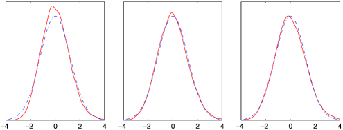
Figure 2: Estimated densities of $\widetilde{T}_{L}(k_{500})$ for $a=500$, $n=3$, and $k_{500}=22$, 105 and 229.

Table 8: Type I errors of order threshold statistics, $\widetilde{T}_{L}(k_{a})$, for different values of the threshold parameter

	$\bolds{[\log^{1/2}a]}$	$\bolds{[\log a]}$	$\bolds{[\log^{3/2}a]}$	$\bolds{[a^{1/2}]}$	$\bolds{[a^{2/3}]}$	$\bolds{[a^{3/4}]}$	$\bolds{[a^{7/8}]}$	$\bolds{a}$
$a=50$ and $n=3$	0.0522	0.0551	0.0601	0.0601	0.0623	0.0635	0.0637	0.0669
$a=50$ and $n=5$	0.0551	0.0583	0.0591	0.0591	0.0588	0.0600	0.0612	0.0619
$a=100$ and $n=3$	0.0506	0.0521	0.0561	0.0563	0.0594	0.0607	0.0617	0.0634
$a=100$ and $n=5$	0.0539	0.0541	0.0541	0.0549	0.0571	0.0578	0.0596	0.0604
$a=200$ and $n=3$	0.0436	0.0440	0.0490	0.0497	0.0552	0.0571	0.0601	0.0597
$a=200$ and $n=5$	0.0548	0.0520	0.0505	0.0504	0.0515	0.0529	0.0542	0.0549
$a=500$ and $n=3$	0.0436	0.0437	0.0452	0.0466	0.0515	0.0558	0.0593	0.0589
$a=500$ and $n=5$	0.0533	0.0492	0.0474	0.0481	0.0510	0.0518	0.0532	0.0534
$a=1000$ and $n=3$	0.0427	0.0403	0.0405	0.0411	0.0475	0.0513	0.0548	0.0557
$a=1000$ and $n=5$	0.0517	0.0486	0.0459	0.0453	0.0466	0.0484	0.0507	0.0521

The results reported in Table 8 are based on 20,000 simulation runs. As expected, the distributions of $\widetilde{T}_{L}(k_{a})$ converge to the normal distribution function and the achieved alpha levels are close to the true value of 0.05. Thus, the asymptotic theory of the order threshold statistics provides a good approximation. More exactly, when the number of groups are larger than 200, all order threshold statistics are robust for the 0.05 significance level. In particular, the achieved alpha level of $\widetilde{T}_{L}(k_{1000})$ is 0.0507 when $a=1000$, $n=5$, and $k_{1000}=[a^{7/8}]=421$.

From now, we compare the empirical power of $\widetilde{T}_{L}(k_{1000})$ using several values of the threshold parameter with that of the classical $F$ statistic. The simulations use samples of size $a=1000$ and $n=5$ generated from the normal distribution with variance 1. The threshold parameter $k_{1000}$ is 20, 50, 100, 250, 500, and 1000. All results are based on 20,000 simulation runs. The alternatives here have 20 of the 1000 $\theta_{i}$ values different from zero. In particular, we consider the following sequence of alternatives indexed by $r$:

$$H_{r}\dvtx\theta_{j}=\eta_{j+r-1}\qquad\mbox{for }j=1,\ldots,1000,r=1,\ldots,20,$$

where $\eta_{j}$, $j=1,2,\ldots,$ is a given sequence. The following are examples with different values of $\bolds\eta$.

Example 4.1.

We generate the values of $\eta_{j}$, $j=1,\ldots,20$, from$\operatorname{Uniform}(-2,2)$. The remaining values of $\eta_{j}$ are 0. The values different from 0 are as follows:

$$(1.8005,-1.0754,0.4274,-0.0561,1.5652,1.0484,$$

$$\hskip 5.4pt-0.1741,-1.9260,1.2856,-0.2212,0.4617,1.1677,1.6873,$$

$$\hskip 8.4pt0.9528,-1.2949,-0.3772,1.7419,1.6676,-0.3589,1.5746).$$

Note that $\#(j\dvtx 0<|\eta_{j}|\leq 1,j=1,2,\ldots)=8$ and $\#(j\dvtx|\eta_{j}|>1,j=1,2,\ldots)=12$.

Example 4.2.

We generate the values of $\eta_{j}$, $j=1,\ldots,20$, from $\operatorname{Exp}(0.7)$. The remaining values of $\eta_{j}$ are 0. The values different from 0 are as follows:

$$(1.0949,0.5511,1.7587,0.1128,0.4033,0.7991,0.6868,$$

$$\hskip 5.4pt0.0993,0.6919,1.8255,1.1272,2.1041,0.3975,$$

$$\hskip 6.8pt1.4730,0.4549,1.5015,0.1830,0.6865,0.1360,2.1458).$$

Note that $\#(j\dvtx 0<\eta_{j}\leq 1,j=1,2,\ldots)=12$, $\#(j\dvtx 1<\eta_{j}\leq 2,j=1,2,\ldots)=6$ and $\#(j\dvtx\eta_{j}>2,j=1,2,\ldots)=2$.

Table 9: Power calculations in Example 4.1

	$\bolds{k_{1000}^{\mathrm{opt}}}$	$\bolds{F_{1000}}$	$\bolds{\widetilde{T}_{L}(20)}$	$\bolds{\widetilde{T}_{L}(50)}$	$\bolds{\widetilde{T}_{L}(100)}$	$\bolds{\widetilde{T}_{L}(250)}$	$\bolds{\widetilde{T}_{L}(500)}$	$\bolds{\widetilde{T}_{L}(1000)}$
$H_{1}$	20	0.8612	0.9992	0.9975	0.9877	0.9482	0.8923	0.8682
$H_{2}$	19	0.7887	0.9963	0.9889	0.9685	0.9000	0.8270	0.7978
$H_{3}$	18	0.7561	0.9957	0.9878	0.9623	0.8762	0.7971	0.7658
$H_{4}$	17	0.7505	0.9952	0.9848	0.9588	0.8743	0.7924	0.7601
$H_{5}$	16	0.7541	0.9949	0.9841	0.9591	0.8801	0.7944	0.7633
$H_{6}$	15	0.6785	0.9901	0.9712	0.9275	0.8175	0.7238	0.6891
$H_{7}$	14	0.6434	0.9859	0.9634	0.9116	0.7856	0.6887	0.6563
$H_{8}$	13	0.6432	0.9855	0.9623	0.9100	0.7876	0.6905	0.6547
$H_{9}$	12	0.5091	0.9422	0.8861	0.8008	0.6505	0.5518	0.5193
$H_{10}$	11	0.4434	0.9191	0.8399	0.7351	0.5794	0.4868	0.4553
$H_{11}$	10	0.4444	0.9191	0.8399	0.7355	0.5742	0.4855	0.4561
$H_{12}$	09	0.4448	0.9230	0.8414	0.7333	0.5760	0.4847	0.4562
$H_{13}$	08	0.3896	0.8894	0.7869	0.6756	0.5132	0.4264	0.4007
$H_{14}$	07	0.2887	0.7710	0.6364	0.5169	0.3835	0.3185	0.2989
$H_{15}$	06	0.2615	0.7437	0.6051	0.4866	0.3537	0.2903	0.2724
$H_{16}$	05	0.2095	0.6603	0.5037	0.3878	0.2803	0.2321	0.2187
$H_{17}$	04	0.2089	0.6560	0.5002	0.3869	0.2742	0.2319	0.2169
$H_{18}$	03	0.1356	0.4002	0.2874	0.2250	0.1686	0.1482	0.1421
$H_{19}$	02	0.0816	0.1736	0.1287	0.1106	0.0943	0.0884	0.0867
$H_{20}$	01	0.0812	0.1743	0.1277	0.1095	0.0934	0.0880	0.0862

Table 10: Power calculations in Example 4.2

	$\bolds{k_{1000}^{\mathrm{opt}}}$	$\bolds{F_{1000}}$	$\bolds{\widetilde{T}_{L}(20)}$	$\bolds{\widetilde{T}_{L}(50)}$	$\bolds{\widetilde{T}_{L}(100)}$	$\bolds{\widetilde{T}_{L}(250)}$	$\bolds{\widetilde{T}_{L}(500)}$	$\bolds{\widetilde{T}_{L}(1000)}$
$H_{1}$	20	0.7680	0.9978	0.9886	0.9657	0.8877	0.8089	0.7769
$H_{2}$	19	0.7275	0.9968	0.9861	0.9550	0.8603	0.7732	0.7366
$H_{3}$	18	0.7241	0.9960	0.9842	0.9533	0.8563	0.7669	0.7330
$H_{4}$	17	0.6278	0.9893	0.9640	0.9048	0.7740	0.6731	0.6394
$H_{5}$	16	0.6253	0.9886	0.9624	0.9052	0.7702	0.6730	0.6373
$H_{6}$	15	0.6188	0.9892	0.9624	0.9031	0.7681	0.6667	0.6306
$H_{7}$	14	0.6011	0.9872	0.9577	0.8891	0.7464	0.6462	0.6119
$H_{8}$	13	0.5871	0.9872	0.9519	0.8829	0.7369	0.6337	0.5982
$H_{9}$	12	0.5831	0.9870	0.9530	0.8819	0.7406	0.6342	0.5962
$H_{10}$	11	0.5614	0.9849	0.9467	0.8730	0.7151	0.6097	0.5750
$H_{11}$	10	0.4476	0.9526	0.8704	0.7600	0.5872	0.4900	0.4598
$H_{12}$	09	0.4009	0.9411	0.8435	0.7224	0.5399	0.4405	0.4121
$H_{13}$	08	0.2521	0.7461	0.5879	0.4612	0.3297	0.2770	0.2612
$H_{14}$	07	0.2495	0.7446	0.5843	0.4573	0.3319	0.2742	0.2597
$H_{15}$	06	0.1831	0.6204	0.4465	0.3361	0.2419	0.2026	0.1913
$H_{16}$	05	0.1820	0.6119	0.4411	0.3383	0.2407	0.2014	0.1898
$H_{17}$	04	0.1283	0.4346	0.2941	0.2197	0.1613	0.1412	0.1356
$H_{18}$	03	0.1296	0.4389	0.2959	0.2195	0.1654	0.1434	0.1363
$H_{19}$	02	0.1195	0.4202	0.2793	0.2084	0.1515	0.1308	0.1258
$H_{20}$	01	0.1176	0.4207	0.2763	0.2041	0.1532	0.1296	0.1238

As expected, the power in each column decreases as $r$ increases and $\widetilde{T}_{L}(20)$ has the highest power. Since the number of $\theta_{i}$’s that are different from zero does not exceed 20, $\widetilde{T}_{L}(20)$ minimizes the accumulation of noise, compared to the other order threshold statistics. For each alternative, the largest power differences between $F_{1000}$ and $\widetilde{T}_{L}(20)$ are about 0.5 (alternative $H_{13}$ in Table 9) and 0.54 (alternative $H_{12}$ in Table 10). In both tables, the power of $\widetilde{T}_{L}(1000)$ is similar to that of $F_{1000}$ because $\widetilde{T}_{L}(1000)$ is a standardized version of $F_{1000}$. Finally, all order threshold statistics achieved higher power than the classical $F$ statistic $F_{1000}$.

4.3 Choosing $k_{a}$

The simulation results and the discussion in the closing paragraph of Section 4.2 suggest that choosing $k_{a}$ equal to the number of groups with nonzero effects, $k_{a}^{\mathrm{opt}}$, maximizes the power. Our recommendation for the choice of the threshold parameter is based again on the idea of Storey (2002, 2003) for enhancing the power of Simes statistic for testing the constructed set of hypothesis testing problems $H_{0}^{(i)}\dvtx\theta_{i}=\overline{X}_{\cdot\cdot}$, $i=1,\ldots,a$, where $\overline{X}_{\cdot\cdot}$ is the overall sample mean. The $p$-value for each hypothesis is approximated by

$$P_{i}=2\bigl{(}1-\Phi(|Z_{i}|)\bigr{)},\qquad i=1,\ldots,a,$$

with

$$Z_{i}=\frac{\overline{X}_{i\cdot}-\overline{X}_{\cdot\cdot}}{\sqrt{S_{p}^{2}/n}},\qquad i=1,\ldots,a,$$

where $\overline{X}_{i\cdot}$ is the sample mean from the $i$th group and $S_{p}^{2}$ is the pooled sample variance. The power-enhanced version of the Simes statistic

$$T_{S}=\min_{1\leq i\leq a}\bigl{\{}aP_{(i)}/i\bigr{\}}$$

rejects the global null hypothesis if $T_{S}<\alpha/(1-\widehat{k}_{a}^{\mathrm{opt}}/a)$, with

$$\widehat{k}_{a}^{\mathrm{opt}}(\lambda)=\max\biggl{\{}\frac{a\mathbb{G}_{a}(\lambda)-a\lambda-1}{1-\lambda},\log^{3/2}a\biggr{\}},$$ (23)

where $\mathbb{G}_{a}$ is the empirical cdf of $\mathbf{P}^{a}=(P_{1},\ldots,P_{a})$, $P_{(1)}<\cdots<P_{(a)}$ are the ordered $P_{i}$’s, and $\lambda$ is the median of the $P_{i}$’s.

The simulation results shown in Table 11 suggest that the power of $\widetilde{T}_{L}(\widehat{k}_{1000}^{\mathrm{opt}})$ is similar to that of $\widetilde{T}_{L}(k_{1000}^{\mathrm{opt}})$. These results are based on 2000 simulation runs; the type I error rate of $\widetilde{T}_{L}(\widehat{k}_{1000}^{\mathrm{opt}})$ was 0.048.

Table 11: Power calculations in Example 4.1

	$\bolds{H_{1}}$	$\bolds{H_{2}}$	$\bolds{H_{3}}$	$\bolds{H_{4}}$	$\bolds{H_{5}}$	$\bolds{H_{6}}$	$\bolds{H_{7}}$	$\bolds{H_{8}}$	$\bolds{H_{9}}$	$\bolds{H_{10}}$
$k_{1000}^{\mathrm{opt}}$	20	19	18	17	16	15	14	13	12	11
$\widetilde{T}_{L}(\widehat{k}_{1000}^{\mathrm{opt}})$	1.000	0.996	0.993	0.994	0.995	0.987	0.980	0.981	0.938	0.904
	$\bolds{H_{11}}$	$\bolds{H_{12}}$	$\bolds{H_{13}}$	$\bolds{H_{14}}$	$\bolds{H_{15}}$	$\bolds{H_{16}}$	$\bolds{H_{17}}$	$\bolds{H_{18}}$	$\bolds{H_{19}}$	$\bolds{H_{20}}$
$k_{1000}^{\mathrm{opt}}$	10	9	8	7	6	5	4	3	2	1
$\widetilde{T}_{L}(\widehat{k}_{1000}^{\mathrm{opt}})$	0.911	0.900	0.883	0.774	0.722	0.674	0.661	0.398	0.182	0.175

5 Discussion

The asymptotic theory of test statistics based on hard and soft thresholding pertain the normal distribution and require the threshold parameter to tend to infinity at a strictly prescribed rate. This second feature results in potentially compromised power of the hard threshold statistic.

Order thresholding, a new thresholding method based on order statistics, is proposed. The asymptotic theory, developed under the normal distribution in this paper, allows great flexibility in the choice of the threshold parameter. A data-driven choice of the order threshold parameter is given. An extension to a one-way HANOVA setting is presented. Simulation studies with normal data suggest that order thresholding can have great power advantage over hard thresholding. Additional simulations with data generated under a one-way HANOVA design suggest even larger power gains over the traditional ANOVA $F$-test.

Applications of the order thresholding approach to testing for the uniform distribution, and to multiple testing problems will be pursued in a follow-up paper.

Appendix A Proof of Theorem 3.1

The proofs of the present lemmas can be found in the archived supplemental material in Kim and Akritas (2010).

A.1 Some auxiliary results

Lemma A.1

Let $U_{i,n}$, $i=1,\ldots,n$, be order statistics from the uniform distribution in $(0,1)$, and set $V_{i,n}=-\log(1-U_{i,n})$. For any $0<\varepsilon<1$ and some $1-\log(n-\sqrt{\frac{n}{2}\log(\frac{58}{\varepsilon})}+1)/\log n\leq\delta(n)<1-\log(\frac{n}{2}\log(\frac{58}{\varepsilon}))/(2\log n)$, set

$$\cases{u_{jn}(\varepsilon)=\cases{\displaystyle\max\Biggl{\{}0,\frac{j}{n}-\sqrt{\frac{1}{2n}\log\biggl{(}\frac{58}{\varepsilon}\biggr{)}}\Biggr{\}},&\quad$1\leq j<n^{1-\delta(n)}$,\vspace*{2pt}\cr\displaystyle 1-e^{-\tilde{\nu}_{jn}}e^{\sqrt{2/\varepsilon}},&\quad$n^{1-\delta(n)}\leq j\leq n$,\cr}\vspace*{2pt}\cr u^{jn}(\varepsilon)=\cases{\displaystyle\frac{j-1}{n}+\sqrt{\frac{1}{2n}\log\biggl{(}\frac{58}{\varepsilon}\biggr{)}},&\quad$1\leq j<n^{1-\delta(n)}$,\vspace*{2pt}\cr\displaystyle 1-e^{-\tilde{\nu}_{jn}}e^{-\sqrt{2/\varepsilon}},&\quad$n^{1-\delta(n)}\leq j\leq n$,}}$$

where $\tilde{\nu}_{jn}=\sum_{i=1}^{j}1/(n-i+1)$. Then, the sequences of constants

$$v_{jn}(\varepsilon)=-\log\bigl{(}1-u_{jn}(\varepsilon)\bigr{)},\qquad v^{jn}(\varepsilon)=-\log\bigl{(}1-u^{jn}(\varepsilon)\bigr{)}$$

satisfy

$$P\{v_{jn}(\varepsilon)<V_{j,n}<v^{jn}(\varepsilon),1\leq j\leq n\}\geq 1-\varepsilon,\qquad n\geq 1.$$ (24)

Lemma A.2

Let $u_{jn}(\varepsilon)$ and $u^{jn}(\varepsilon)$ be given in Lemma A.1. Then, the sequences of constants $u_{jn}(\varepsilon)$ and $u^{jn}(\varepsilon)$, $j=1,\ldots,n$, satisfy the relation

$$u_{jn}(\varepsilon)<\frac{j}{n+1}<u^{jn}(\varepsilon).$$

Assume that $1-n^{-\delta(n)}\to 0$, as $n\to\infty$. Then, the sequences of constants $u_{jn}(\varepsilon)$ and $u^{jn}(\varepsilon)$, given in Lemma A.1, satisfy the relation $\sup_{1\leq j\leq n}(u^{jn}(\varepsilon)-u_{jn}(\varepsilon))=o(1)$ (cf. Glivenko–Cantelli theorem). If we take all $u_{jn}(\varepsilon)$ and $u^{jn}(\varepsilon)$ from the Kolmogorov’s inequality, then $u_{jn}(\varepsilon)=1-e^{-\tilde{\nu}_{jn}+\sqrt{2/\varepsilon}}$ and $u^{jn}(\varepsilon)=1-e^{-\tilde{\nu}_{jn}-\sqrt{2/\varepsilon}}$, $j=1,\ldots,n$. Under these settings, $\sup_{1\leq j\leq n}(u^{jn}(\varepsilon)-u_{jn}(\varepsilon))\neq o(1)$. Also, the positive function $R(j)$, defined in Lemma A.4, is not increasing on $1\leq j\leq n$.

Lemma A.3

Let $\tilde{\nu}_{jn}$ be given in Lemma A.1, and let $\nu_{jn}=-\log(1-j/(n+1))$, $j=1,\ldots,n$. Assume that $1-n^{-\delta(n)}\to 0$ and $n^{1/2}(1-n^{-\delta(n)})\to\infty$, as $n\to\infty$. Then, the sequences of constants $v_{jn}(\varepsilon)$ and $v^{jn}(\varepsilon)$, given in Lemma A.1, satisfy the relations

$$v_{jn}(\varepsilon)<\nu_{jn}<\tilde{\nu}_{jn}<v^{jn}(\varepsilon)\quad\mbox{and}\quad v^{jn}(\varepsilon)-v_{jn}(\varepsilon)\leq K(\varepsilon),$$

where $K(\varepsilon)$ is independent of $n$.

Lemma A.4

Let $v_{yn}(\varepsilon)$ and $v^{yn}(\varepsilon)$, $1\leq y\leq n$, be given in Lemma A.1, and let $\tilde{H}=F^{-1}\circ G$, where $F$ is the central chi-squared distribution function with 1 degree of freedom and $G$ is the standard exponential distribution function. Then,

1. $\tilde{H}^{\prime}$ is increasing, positive, concave, and $\tilde{H}^{\prime}(v)\to 2$, as $v\to\infty$.

2. $\tilde{H}^{\prime\prime}$ is a decreasing positive function, and $\tilde{H}^{\prime\prime}(v)\to 0$, as $v\to\infty$.

3. $\tilde{H}(v)\tilde{H}^{\prime\prime}(v)\to 0$, as $v\to\infty$.

4. $\frac{\tilde{H}^{\prime\prime\prime}(v)}{\tilde{H}^{\prime\prime}(v)}(1-e^{-v})\to 0$, as $v\to 0$, and $\frac{\tilde{H}^{\prime\prime\prime}(v)}{\tilde{H}^{\prime\prime}(v)}\to 0$, as $v\to\infty$.

5. Assume that $1-n^{-\delta(n)}\to 0$ and $n^{1/2}(1-n^{-\delta(n)})\to\infty$, as $n\to\infty$. The positive function

   $$R(y)=\bigl{(}v^{yn}(\varepsilon)-v_{yn}(\varepsilon)\bigr{)}\tilde{H}^{\prime\prime}(v_{yn}(\varepsilon))\sqrt{\frac{y}{n-y+1}}$$

   is increasing on $1\leq y<n^{1-\delta(n)}$. Moreover, for sufficiently large $n$, $R(y)$ is also increasing on $n^{1-\delta(n)}\leq y\leq n$.

A.2 Proof of Theorem 3.1

We need to check Assumptions A, B and C of CGJ1967. We use the original forms of Assumptions A and C (restate below for convenience), but a slightly stronger version of Assumption B. [Note that the simultaneous bounds of the exponential order statistics, $v_{jn}(\varepsilon)$ and $v^{jn}(\varepsilon)$ used in Assumption B, are different from those in CGJ1967.]

Assumption A: $\tilde{H}(v)$ is continuously differentiable for $0<v<\infty$.

Assumption B: For each $\varepsilon>0$,

$$A_{n} = \sum_{j=n-k_{n}+1}^{n}\Biggl{[}\Bigl{\{}{\sup_{v_{jn}(\varepsilon)<v<v^{jn}(\varepsilon)}}|\tilde{H}^{\prime}(v)-\tilde{H}^{\prime}(\tilde{\nu}_{jn})|\Bigr{\}}\sqrt{\frac{j}{n-j+1}}\Biggr{]}$$

$$= o(n\sigma_{n}(k_{n})),$$

where $v_{jn}(\varepsilon)$, $v^{jn}(\varepsilon)$, and $\tilde{\nu}_{jn}$ are given in Lemma A.1.

Assumption C: ${\max_{1\leq j\leq n}}|\alpha_{jn}(k_{n})|=o(n^{1/2}\sigma_{n}(k_{n}))$.

Assumption A is clearly satisfied. To verify Assumption C, use Lemma A.4(1) to write

$$\frac{{\max_{1\leq j\leq n}}|\alpha_{jn}(k_{n})|}{\sqrt{n}\sigma_{n}(k_{n})} = \frac{\tilde{H}^{\prime}(\tilde{\nu}_{nn})}{\sqrt{\sum_{j=1}^{n}\alpha_{jn}^{2}(k_{n})}}$$

$$\leq \frac{2}{\sqrt{\sum_{j=n-k_{n}+1}^{n}\{\tilde{H}^{\prime}(\tilde{\nu}_{jn})\}^{2}}}.$$

Suppose first that $k_{n}/n\rightarrow 0$ as $n\rightarrow\infty$. Then

$$\sum_{j=n-k_{n}+1}^{n}\{\tilde{H}^{\prime}(\tilde{\nu}_{jn})\}^{2}\geq k_{n}\{\tilde{H}^{\prime}(\tilde{\nu}_{n-k_{n}+1,n})\}^{2}\to\infty\qquad\mbox{as }n\to\infty,$$

so that (A.2) tends to zero and Assumption C is satisfied in this case. Next, suppose that $k_{n}/n\to r$ as $n\rightarrow\infty$, for some $0<r\leq 1$. Using the approximation (2.9) of CGJ1967, that is, $\tilde{\nu}_{jn}\simeq\nu_{jn}=-\log(1-j/(n+1))$, it follows that

$$\frac{1}{n}\sum_{j=n-k_{n}+1}^{n}\{\tilde{H}^{\prime}(\tilde{\nu}_{jn})\}^{2}$$

$$\qquad\simeq\frac{1}{n}\sum_{j=1}^{n}I\biggl{(}\frac{j}{n+1}>\frac{n-k_{n}}{n+1}\biggr{)}\biggl{\{}\biggl{(}1-\frac{j}{n+1}\biggr{)}(F^{-1})^{\prime}\biggl{(}\frac{j}{n+1}\biggr{)}\biggr{\}}^{2}$$

$$\qquad\to\int_{0}^{1}I(t>1-r)\biggl{\{}\frac{(1-t)}{f(F^{-1}(t))}\biggr{\}}^{2}\,dt>0\qquad\mbox{as }n\to\infty,$$

so that Assumption C is also satisfied. To show Assumption B, we use Lemmas A.4(1) and A.3 to write ${\sup_{v_{jn}(\varepsilon)<v<v^{jn}(\varepsilon)}}|\tilde{H}^{\prime}(v)-\tilde{H}^{\prime}(\tilde{\nu}_{jn})|\leq\tilde{H}^{\prime}(v^{jn}(\varepsilon))-\tilde{H}^{\prime}(v_{jn}(\varepsilon))=(v^{jn}(\varepsilon)-v_{jn}(\varepsilon))\tilde{H}^{\prime\prime}(\tilde{v}_{jn}(\varepsilon))$, $\tilde{v}_{jn}(\varepsilon)\in(v_{jn}(\varepsilon),v^{jn}(\varepsilon))$. Thus,

$$\qquad\quad\frac{A_{n}}{n\sigma_{n}(k_{n})} \leq \frac{1}{\sqrt{n}}\sum_{j=n-k_{n}+1}^{n}\Biggl{[}\bigl{\{}\bigl{(}v^{jn}(\varepsilon)-v_{jn}(\varepsilon)\bigr{)}\tilde{H}^{\prime\prime}(v_{jn}(\varepsilon))\bigr{\}}\sqrt{\frac{j}{n-j+1}}\Biggr{]}$$

$${}\times\Biggl{(}\sqrt{\sum_{j=n-k_{n}+1}^{n}\{\tilde{H}^{\prime}(\tilde{\nu}_{jn})\}^{2}}\Biggr{)}^{-1},$$

where the inequality is justified by the fact that $\tilde{H}^{\prime\prime}$ is a decreasing positive function [Lemma A.4(2)]. We need to prove that (A.2) tends to zero as $n\to\infty$. Suppose first that $k_{n}/n\to 0$, as $n\rightarrow\infty$. Divide numerator and denominator of (A.2) by $k_{n}^{1/2}$ and consider first the numerator. Then,

$$\frac{1}{\sqrt{nk_{n}}}\sum_{j=n-k_{n}+1}^{n}\Biggl{[}\bigl{\{}\bigl{(}v^{jn}(\varepsilon)-v_{jn}(\varepsilon)\bigr{)}\tilde{H}^{\prime\prime}(v_{jn}(\varepsilon))\bigr{\}}\sqrt{\frac{j}{n-j+1}}\Biggr{]}$$

$$\qquad=\cases{\displaystyle\sqrt{\frac{8}{\varepsilon}}\dfrac{1}{\sqrt{nk_{n}}}\sum_{j=n-k_{n}+1}^{n}\Biggl{[}\tilde{H}^{\prime\prime}(v_{jn}(\varepsilon))\sqrt{\frac{j}{n-j+1}}\Biggr{]},\cr\qquad\mbox{if $\displaystyle k_{n}<\sqrt{\frac{n}{2}\log\biggl{(}\frac{58}{\varepsilon}\biggr{)}}$},\cr\displaystyle\frac{1}{\sqrt{nk_{n}}}\sum_{j=n-k_{n}+1}^{n^{1-\delta(n)}-1}\Biggl{[}\bigl{\{}\bigl{(}v^{jn}(\varepsilon)-v_{jn}(\varepsilon)\bigr{)}\tilde{H}^{\prime\prime}(v_{jn}(\varepsilon))\bigr{\}}\sqrt{\frac{j}{n-j+1}}\Biggr{]}\cr\displaystyle\qquad{}+\frac{1}{\sqrt{nk_{n}}}\sum_{j=n^{1-\delta(n)}}^{n-k_{n}^{1/4}}\Biggl{[}\bigl{\{}\bigl{(}v^{jn}(\varepsilon)-v_{jn}(\varepsilon)\bigr{)}\tilde{H}^{\prime\prime}(v_{jn}(\varepsilon))\bigr{\}}\sqrt{\frac{j}{n-j+1}}\Biggr{]}\cr\displaystyle\qquad{}+\frac{1}{\sqrt{nk_{n}}}\sum_{j=n-k_{n}^{1/4}+1}^{n}\Biggl{[}\bigl{\{}\bigl{(}v^{jn}(\varepsilon)-v_{jn}(\varepsilon)\bigr{)}\tilde{H}^{\prime\prime}(v_{jn}(\varepsilon))\bigr{\}}\sqrt{\frac{j}{n-j+1}}\Biggr{]},\cr\qquad\mbox{otherwise},}$$

with $1-\log(n-\sqrt{\frac{n}{2}\log(\frac{58}{\varepsilon})}+1)/\log n\leq\delta(n)<1-\log(n-c_{\varepsilon}n^{3/16}k_{n}^{5/8}+1)/\log n$ [This range is applied only when $k_{n}\geq\sqrt{\frac{n}{2}\log(\frac{58}{\varepsilon})}$]. Assume that $1-n^{-\delta(n)}\to 0$, $n^{1/2}(1-n^{-\delta(n)})\to\infty$, and $n^{1/2}(1-n^{-\delta(n)})^{3/2}\to d$ for some $d>0$, as $n\to\infty$. If $k_{n}<\sqrt{\frac{n}{2}\log(\frac{58}{\varepsilon})}$, then $\frac{1}{\sqrt{nk_{n}}}\sum_{j=n-k_{n}+1}^{n}[\tilde{H}^{\prime\prime}(v_{jn}(\varepsilon))\sqrt{\frac{j}{n-j+1}}]<(\frac{1}{2}\log(\frac{58}{\varepsilon}))^{1/4}n^{1/4}\tilde{H}^{\prime\prime}(v_{nn}(\varepsilon))\to 0$, as $n\to\infty$. This inequality is justified by Lemma A.4(5), and the fact that $n^{1/4}\tilde{H}^{\prime\prime}(v_{nn}(\varepsilon))$ tends to zero. Suppose that $k_{n}\geq\sqrt{\frac{n}{2}\log(\frac{58}{\varepsilon})}$ and $k_{n}/n\to 0$, as $n\to\infty$. Set $a_{n}=n^{1-\delta(n)}-1$ and $b_{n}=n-k_{n}^{1/4}$. Using Lemmas A.4(5) and A.3, we have

$$\frac{1}{\sqrt{nk_{n}}}\sum_{j=n-k_{n}+1}^{n}\Biggl{[}\bigl{\{}\bigl{(}v^{jn}(\varepsilon)-v_{jn}(\varepsilon)\bigr{)}\tilde{H}^{\prime\prime}(v_{jn}(\varepsilon))\bigr{\}}\sqrt{\frac{j}{n-j+1}}\Biggr{]}$$

$$\qquad\leq\sqrt{\frac{k_{n}}{n(1-n^{-\delta(n)})}}\bigl{(}v^{a_{n},n}(\varepsilon)-v_{a_{n},n}(\varepsilon)\bigr{)}\tilde{H}^{\prime\prime}(v_{a_{n},n}(\varepsilon))$$ (27)

$$\qquad\quad{}+c_{\varepsilon}\sqrt{\frac{8}{\varepsilon}}n^{3/16}\tilde{H}^{\prime\prime}(v_{b_{n},n}(\varepsilon))+\sqrt{\frac{8}{\varepsilon}}k_{n}^{-1/4}\tilde{H}^{\prime\prime}(v_{nn}(\varepsilon)).$$ (28)

Since $(n-a_{n}+1)/n^{1/2}\to\infty$ as $n\to\infty$, using a one-term Taylor expansion we have $v^{a_{n},n}(\varepsilon)-v_{a_{n},n}(\varepsilon)\approx\frac{\sqrt{2n\log({58}/{\varepsilon})}-1}{n-a_{n}+1-\sqrt{{n}/{2}\log({58}/{\varepsilon})}}=O(\frac{1}{n^{1/2}(1-n^{-\delta(n)})})$. Thus, we have

$$\mbox{(\ref{pf1.1})}=O\biggl{(}\frac{1}{n^{1/2}(1-n^{-\delta(n)})^{3/2}}\cdot\frac{k_{n}^{1/2}}{n^{1/2}}\tilde{H}^{\prime\prime}(v_{a_{n},n}(\varepsilon))\biggr{)}\to 0\qquad\mbox{as }n\to\infty,$$

where it is justified by Lemma A.4(2) and the fact that $v_{a_{n},n}(\varepsilon)$ tends to infinity. From Lemma A.4(2), the second term of (28) tends to 0 as $n\to\infty$. Moreover, the first term of (28) tends to 0 as $n\to\infty$ (even $b_{n}=n-n^{1/4}$). Since also $(\frac{1}{k_{n}}\sum_{j=n-k_{n}+1}^{n}\{\tilde{H}^{\prime}(\tilde{\nu}_{jn})\}^{2})^{-1/2}\leq(\tilde{H}^{\prime}(\tilde{\nu}_{n-k_{n}+1,n}))^{-1}<\infty$, (A.2) tends to zero and Assumption B is satisfied when $k_{n}/n\to 0$ as $n\to\infty$. Next, we suppose that for some $0<r\leq 1$, $k_{n}/n\to r$ as $n\rightarrow\infty$. Divide numerator and denominator of (A.2) by $n^{1/2}$ and consider the numerator and denominator separately. Since

$$\frac{1}{n}\sum_{j=n-k_{n}+1}^{n}\Biggl{[}\bigl{\{}\bigl{(}v^{jn}(\varepsilon)-v_{jn}(\varepsilon)\bigr{)}\tilde{H}^{\prime\prime}(v_{jn}(\varepsilon))\bigr{\}}\sqrt{\frac{j}{n-j+1}}\Biggr{]}$$

$$\qquad\leq O\biggl{(}\frac{\tilde{H}^{\prime\prime}(v_{n^{1-\delta(n)}-1,n}(\varepsilon))}{n^{1/2}(1-n^{-\delta(n)})^{3/2}}\biggr{)}+\sqrt{\frac{8}{\varepsilon}}n^{3/16}\tilde{H}^{\prime\prime}(v_{n-n^{1/4},n}(\varepsilon))$$

$$\qquad\quad{}+\sqrt{\frac{8}{\varepsilon}}n^{-1/4}\tilde{H}^{\prime\prime}(v_{nn}(\varepsilon))$$

$$\qquad\to 0\qquad\mbox{as }n\to\infty,$$

which can be obtained by breaking up the summation first for $j=n-k_{n}+1$ to $n^{1-\delta(n)}-1$, $n^{1-\delta(n)}$ to $n-n^{1/4}$, and lastly $n-n^{1/4}+1$ to $n$ with $1-\log(n-\sqrt{\frac{n}{2}\log(\frac{58}{\varepsilon})}+1)/\log n\leq\delta(n)<1-\log(n-n^{13/16}+1)/\log n$, and $(\frac{1}{n}\sum_{j=n-k_{n}+1}^{n}\{\tilde{H}^{\prime}(\tilde{\nu}_{jn})\}^{2})^{-1/2}<\infty$, the term (A.2) converges to 0 as $n\to\infty$ in this case. Thus, Assumption B holds for both cases. Since Assumptions A, B and C of CGJ1967 are satisfied, the proof is done.

Appendix B Proof of Theorem 4.1

The proofs of the present lemmas can be found in the archived supplemental material in Kim and Akritas (2010).

B.1 Some auxiliary results

Lemma B.1

For any $0<\varepsilon<1$ and some $\delta(a)$ which satisfies $1-\log(a-\sqrt{\frac{a}{2}\log(\frac{58}{\varepsilon})}+1)/\log a\leq\delta(a)<1-\log(\frac{a}{2}\log(\frac{58}{\varepsilon}))/(2\log a)$, $1-a^{-\delta(a)}\to 0$, $a^{1/2}(1-a^{-\delta(a)})\to\infty$, and $a^{1/2}(1-a^{-\delta(a)})^{3/2}\to d$ for some $d>0$, as $a\to\infty$, let

$$\cases{u_{ja}(\varepsilon)=\cases{\displaystyle\max\Biggl{\{}0,\frac{j}{a}-\sqrt{\frac{1}{2a}\log\biggl{(}\frac{58}{\varepsilon}\biggr{)}}\Biggr{\}},&\quad$1\leq j<a^{1-\delta(a)}$,\vspace*{2pt}\cr\displaystyle 1-e^{-\tilde{\nu}_{ja}}e^{\sqrt{2/\varepsilon}},&\quad$a^{1-\delta(a)}\leq j\leq a$,}\vspace*{2pt}\cr u^{ja}(\varepsilon)=\cases{\displaystyle\frac{j-1}{a}+\sqrt{\frac{1}{2a}\log\biggl{(}\frac{58}{\varepsilon}\biggr{)}},&\quad$1\leq j<a^{1-\delta(a)}$,\vspace*{2pt}\cr\displaystyle 1-e^{-\tilde{\nu}_{ja}}e^{-\sqrt{2/\varepsilon}},&\quad$a^{1-\delta(a)}\leq j\leq a$,}}$$

where $\tilde{\nu}_{ja}=\sum_{i=1}^{j}1/(a-i+1)$, and set

$$v_{ja}(\varepsilon)=-\log\bigl{(}1-u_{ja}(\varepsilon)\bigr{)},\qquad v^{ja}(\varepsilon)=-\log\bigl{(}1-u^{ja}(\varepsilon)\bigr{)}.$$

For any $M\geq 0$, let $\tilde{H}_{a,M}(v)=G_{a,M}^{-1}(1-e^{-v})$, where $G_{a,M}$ is the noncentral chi-squared distribution function with 1 degree of freedom and noncentrality parameter $M^{2}/a$. Then,

1. $\tilde{H}_{a,M}^{\prime}$ is bounded and $\tilde{H}_{a,M}^{\prime}(v)\to 2$, as $v\to\infty$ and $a\to\infty$.

2. $\tilde{H}_{a,M}^{\prime\prime}(v)=B_{a,M}(v)-(\tilde{H}_{a,M}^{\prime}(v))^{2}J_{a,M}(v)$, where

   $$B_{a,M}(v) = -\tilde{H}_{a,M}^{\prime}(v)+(\tilde{H}_{a,M}^{\prime}(v))^{2}\biggl{(}\frac{1}{2}+\frac{1}{2\tilde{H}_{a,M}(v)}\biggr{)},$$

   $$J_{a,M}(v) = \frac{\sum_{k=1}^{\infty}\{{(M^{2}/a)^{k}(\tilde{H}_{a,M}(v))^{k-1}}/({2^{2k}(k-1)!\Gamma(k+1/2)})\}}{\sum_{k=0}^{\infty}\{{(M^{2}/a)^{k}(\tilde{H}_{a,M}(v))^{k}}/({2^{2k}k!\Gamma(k+1/2)})\}}.$$

   Note that $B_{a,M}$ is a decreasing positive function, $B_{a,M}(v)\to 0$ as $v\to\infty$ and $a\to\infty$, and $J_{a,M}$ is bounded by $M^{2}/(2a)$.

3. The positive function

   $$R_{M}(y)=\bigl{(}v^{ya}(\varepsilon)-v_{ya}(\varepsilon)\bigr{)}B_{a,M}(v_{ya}(\varepsilon))\sqrt{\frac{y}{a-y+1}}$$

   is increasing on $1\leq y<a^{1-\delta(a)}$. Moreover, for sufficiently large $a$, $R_{M}(y)$ is also increasing on $a^{1-\delta(a)}\leq y\leq a$.

Lemma B.2

Consider the setting of Lemma B.1. Let $g_{a,0}$ and $g_{a,M}$ be the density functions of $\chi_{1}^{2}(0)$ and $\chi^{2}_{1}(M^{2}/a)$, respectively. Set $y_{a,0}=\tilde{H}_{a,0}(v_{aa}(\varepsilon))=G_{a,0}^{-1}(1-e^{-v_{aa}(\varepsilon)})$ and $y_{a,M}=\tilde{H}_{a,M}(v_{aa}(\varepsilon))=G_{a,M}^{-1}(1-e^{-v_{aa}(\varepsilon)})$. Then,

1. $y_{a,M}$ is bounded by $(2\log(a+1)-2\log(\sqrt{\pi/2})+2\log(e^{M/(2\sqrt{a})}+\break e^{-M/(2\sqrt{a})}))^{2}$.

2. $g_{a,0}(y_{a,M})/g_{a,M}(y_{a,M})\to 1$ and $a^{1/4}(g_{a,0}(y_{a,M})/g_{a,M}(y_{a,M})-1)\to 0$, as $a\to\infty$.

3. $\frac{g_{a,0}(y_{a,0})-g_{a,0}(y_{a,M})}{g_{a,0}(y_{a,M})}\approx-(\frac{y_{a,M}^{-1}+1}{2})\frac{M^{2}}{2a}C_{a,M}$, where $C_{a,M}$ is defined in the proof. In particular, $C_{a,M}=O(y_{a,M})$.

4. $a^{1/4}(y_{a,0}/y_{a,M}-1)\to 0$ and $a^{1/4}(g_{a,0}(y_{a,0})/g_{a,0}(y_{a,M})-1)\to 0$, as $a\to\infty$.

5. $a^{1/4}(e^{-v_{aa}(\varepsilon)}/g_{a,0}(y_{a,M})-2+2/y_{a,0})\to 0$, as $a\to\infty$.

6. $a^{1/4}(e^{-v_{aa}(\varepsilon)}/g_{a,M}(y_{a,M})-2+2/y_{a,M})\to 0$, as $a\to\infty$.

For any $M\geq 0$, we write $\tilde{H}^{\prime}_{a,M}(v_{aa}(\varepsilon))=\frac{e^{-v_{aa}(\varepsilon)}}{g_{a,M}(y_{a,M})}$ and$B_{a,M}(v_{aa}(\varepsilon))=\frac{e^{-v_{aa}(\varepsilon)}}{2g_{a,M}(y_{a,M})}$ $(\frac{e^{-v_{aa}(\varepsilon)}}{g_{a,M}(y_{a,M})}-2+\frac{e^{-v_{aa}(\varepsilon)}}{g_{a,M}(y_{a,M})}\cdot\frac{1}{y_{a,M}})$. From Lemmas B.1(1), B.1(2) and B.2(6), we obtain that $a^{1/4}B_{a,M}(v_{aa}(\varepsilon))\to 0$, as $a\to\infty$.

Lemma B.3

Consider the setting of Lemma B.2. Let $b_{a}=a-k_{a}^{1/4}$ with $k_{a}\geq\sqrt{\frac{a}{2}\log(\frac{58}{\varepsilon})}$. Set $x_{a,0}=\tilde{H}_{a,0}(v_{b_{a},a}(\varepsilon))=G_{a,0}^{-1}(1-e^{-v_{b_{a},a}(\varepsilon)})$ and $x_{a,M}=\tilde{H}_{a,M}(v_{b_{a},a}(\varepsilon))=G_{a,M}^{-1}(1-e^{-v_{b_{a},a}(\varepsilon)})$. Then,

1. $x_{a,M}\leq(2\log(a+1)-2\log(k_{a}^{1/4}+1)-2\log(\sqrt{\pi/2})+2\log(e^{M/(2\sqrt{a})}+e^{-M/(2\sqrt{a})}))^{2}$.

2. $g_{a,0}(x_{a,M})/g_{a,M}(x_{a,M})\to 1$ and $a^{3/16}(g_{a,0}(x_{a,M})/g_{a,M}(x_{a,M})-1)\to 0$, as $a\to\infty$.

3. $\frac{g_{a,0}(x_{a,0})-g_{a,0}(x_{a,M})}{g_{a,0}(x_{a,M})}\approx-(\frac{x_{a,M}^{-1}+1}{2})\frac{M^{2}}{2a}C^{\prime}_{a,M}$, where

   $$C^{\prime}_{a,M}=\frac{\phi^{\prime}(\sqrt{x_{a,M}}-t^{*}/\sqrt{a})+\phi^{\prime}(\sqrt{x_{a,M}}+t^{*}/\sqrt{a})}{g_{a,0}(x_{a,\tilde{t}})}\qquad\mbox{with }t^{*},\tilde{t}\in(0,M).$$

   In particular, $C^{\prime}_{a,M}=O(x_{a,M})$.

4. $a^{3/16}(x_{a,0}/x_{a,M}-1)\to 0$ and $a^{3/16}(g_{a,0}(x_{a,0})/g_{a,0}(x_{a,M})-1)\to 0$, as $a\to\infty$.

5. $a^{3/16}(e^{-v_{b_{a},a}(\varepsilon)}/g_{a,0}(x_{a,M})-2+2/x_{a,0})\to 0$, as $a\to\infty$.

6. $a^{3/16}(e^{-v_{b_{a},a}(\varepsilon)}/g_{a,M}(x_{a,M})-2+2/x_{a,M})\to 0$, as $a\to\infty$.

From Lemmas B.1(1), B.1(2), and B.3(6), we obtain that $a^{3/16}\times B_{a,M}(v_{a-k_{a}^{1/4},a}(\varepsilon))\to 0$, as $a\to\infty$.

B.2 Proof of Theorem 4.1

For simplicity, let $\tilde{H}_{a,t}(v)=G_{a,t}^{-1}(1-e^{-v})$. Then

$$\alpha_{ia}^{t}(k_{a})=\frac{1}{a-i+1}\sum_{j=i}^{a}c_{ja}\frac{e^{-\tilde{\nu}_{ja}}}{g_{a,t}(G_{a,t}^{-1}(1-e^{-\tilde{\nu}_{ja}}))}=\frac{1}{a-i+1}\sum_{j=i}^{a}c_{ja}\tilde{H}_{a,t}^{\prime}(\tilde{\nu}_{ja})$$

and

$$(\sigma_{a}^{t}(k_{a}))^{2}=\frac{1}{a}\sum_{i=1}^{a}(\alpha_{ia}^{t}(k_{a}))^{2}.$$

Let us check Assumptions A, B and C of CGJ1967, which we restated in the proof of Theorem 3.1. For given any $|t|<M$, Assumption A is clearly satisfied. Next, it is easily verified that for any fixed values of $a$ and $v$, $\tilde{H}^{\prime}_{a,t}(v)$ increases as $|t|$ increases. Thus, $\alpha_{ia}^{t}(k_{a})$ and $\sigma_{a}^{t}(k_{a})$ increase as $|t|$ increases. Let us check Assumption C: for given any $|t|<M$,

$$\frac{{\max_{1\leq j\leq a}}|\alpha_{ja}^{t}(k_{a})|}{\sqrt{a}\sigma_{a}^{t}(k_{a})} \leq \frac{{\max_{1\leq j\leq a}}|\alpha_{ja}^{M}(k_{a})|}{\sqrt{a}\sigma_{a}^{0}(k_{a})}$$

$$\leq \frac{\max_{a-k_{a}+1\leq j\leq a}\tilde{H}^{\prime}_{a,M}(\tilde{\nu}_{ja})}{\sqrt{\sum_{j=a-k_{a}+1}^{a}\{\tilde{H}_{a,0}^{\prime}(\tilde{\nu}_{ja})\}^{2}}}$$

$$\to 0\qquad\mbox{as }a\to\infty,$$

provided that $k_{a}\to\infty$, as $a\to\infty$. It is justified by the facts that

$$\max_{a-k_{a}+1\leq j\leq a}\tilde{H}^{\prime}_{a,M}(\tilde{\nu}_{ja})$$

is bounded [Lemma B.1(1)] and $\sum_{j=a-k_{a}+1}^{a}\{\tilde{H}_{a,0}^{\prime}(\tilde{\nu}_{ja})\}^{2}\to\infty$ as $k_{a}$ tends to infinity with $a$. (It was shown in the proof of Theorem 3.1 because it becomes the central chi-square case when $t=0$.) In order to verify Assumption B, it suffices to show that

$$\frac{\sum_{j=a-k_{a}+1}^{a}[\{{\sup_{v_{ja}(\varepsilon)<v<v^{ja}(\varepsilon)}}|\tilde{H}_{a,M}^{\prime}(v)-\tilde{H}_{a,M}^{\prime}(\tilde{\nu}_{ja})|\}\sqrt{{j}/({a-j+1})}]}{\sqrt{a\sum_{j=a-k_{a}+1}^{a}\{\tilde{H}_{a,0}^{\prime}(\tilde{\nu}_{ja})\}^{2}}}=o(1),$$

where $v_{ja}(\varepsilon)$, $v^{ja}(\varepsilon)$, and $\tilde{\nu}_{ja}$ are given in Lemma B.1. Using Lemma B.1(2), we write

$${\sup_{v_{ja}(\varepsilon)<v<v^{ja}(\varepsilon)}}|\tilde{H}_{a,M}^{\prime}(v)-\tilde{H}_{a,M}^{\prime}(\tilde{\nu}_{ja})|$$

$$\qquad\leq\bigl{(}v^{ja}(\varepsilon)-v_{ja}(\varepsilon)\bigr{)}\cdot|\tilde{H}_{a,M}^{\prime\prime}(v_{ja}^{*})|$$

$$\qquad\leq\bigl{(}v^{ja}(\varepsilon)-v_{ja}(\varepsilon)\bigr{)}B_{a,M}(v_{ja}(\varepsilon))$$

$$\qquad\quad{}+\bigl{(}v^{ja}(\varepsilon)-v_{ja}(\varepsilon)\bigr{)}(\tilde{H}_{a,M}^{\prime}(v_{ja}^{*}))^{2}M^{2}/(2a)$$

with some $v_{ja}^{*}\in(v_{ja}(\varepsilon),v^{ja}(\varepsilon))$. From the above inequality, we have

$$\frac{\sum_{j=a-k_{a}+1}^{a}[\{{\sup_{v_{ja}(\varepsilon)<v<v^{ja}(\varepsilon)}}|\tilde{H}_{a,M}^{\prime}(v)-\tilde{H}_{a,M}^{\prime}(\tilde{\nu}_{ja})|\}\sqrt{{j}/({a-j+1})}]}{\sqrt{a\sum_{j=a-k_{a}+1}^{a}\{\tilde{H}_{a,0}^{\prime}(\tilde{\nu}_{ja})\}^{2}}}$$

$$\qquad\leq\frac{{1}/{\sqrt{a}}\sum_{j=a-k_{a}+1}^{a}[\{(v^{ja}(\varepsilon)-v_{ja}(\varepsilon))B_{a,M}(v_{ja}(\varepsilon))\}\sqrt{{j}/({a-j+1})}]}{\sqrt{\sum_{j=a-k_{a}+1}^{a}\{\tilde{H}_{a,0}^{\prime}(\tilde{\nu}_{ja})\}^{2}}}$$

$$\qquad\quad{}+\frac{1}{\sqrt{a}}\sum_{j=a-k_{a}+1}^{a}\Biggl{[}\biggl{\{}\bigl{(}v^{ja}(\varepsilon)-v_{ja}(\varepsilon)\bigr{)}(\tilde{H}_{a,M}^{\prime}(v_{ja}^{*}))^{2}\frac{M^{2}}{2a}\biggr{\}}\sqrt{\frac{j}{a-j+1}}\Biggr{]}$$

$$\qquad\quad\hskip 11.0pt{}\times\Biggl{(}{\sqrt{\sum_{j=a-k_{a}+1}^{a}\{\tilde{H}_{a,0}^{\prime}(\tilde{\nu}_{ja})\}^{2}}}\Biggr{)}^{-1}.$$

To show that (B.2) tends to zero, we use Lemmas B.1(1) and A.3 to write

$$\mbox{(\ref{subproof-2.9.1})}\leq C_{\varepsilon}\cdot\frac{k_{a}}{a}\cdot\Biggl{(}\sum_{j=a-k_{a}+1}^{a}\{\tilde{H}_{a,0}^{\prime}(\tilde{\nu}_{ja})\}^{2}\Biggr{)}^{-1/2}\qquad\mbox{for some }0<C_{\varepsilon}<\infty.$$

Suppose first that $k_{a}/a\to 0$ as $a\to\infty$. Then

$$\Biggl{(}\frac{1}{k_{a}}\sum_{j=a-k_{a}+1}^{a}\{\tilde{H}_{a,0}^{\prime}(\tilde{\nu}_{ja})\}^{2}\Biggr{)}^{-1/2}\leq\frac{1}{\tilde{H}^{\prime}_{a,0}(\tilde{\nu}_{a-k_{a}+1,a})}<\infty,$$ (31)

so that (B.2) tends to 0 as $a\to\infty$. For some $0<r\leq 1$, if $k_{a}/a\to r$ as $a\to\infty$, then

$$\Biggl{(}\frac{1}{a}\sum_{j=a-k_{a}+1}^{a}\{\tilde{H}_{a,0}^{\prime}(\tilde{\nu}_{ja})\}^{2}\Biggr{)}^{-1/2}<\infty.$$ (32)

Thus, (B.2) tends to 0 as $a\to\infty$ in both cases. Since (B.2) converges to zero, the remaining part is to prove that (B.2) tends to 0, provided that $k_{a}\to\infty$ as $a\to\infty$. Suppose first that $k_{a}<\sqrt{\frac{a}{2}\log(\frac{58}{\varepsilon})}$. Divide numerator and denominator of (B.2) by $k_{a}^{1/2}$ and consider first the numerator. From Lemma B.1(3), we have

$$\frac{1}{\sqrt{ak_{a}}}\sum_{j=a-k_{a}+1}^{a}\Biggl{[}\bigl{\{}\bigl{(}v^{ja}(\varepsilon)-v_{ja}(\varepsilon)\bigr{)}B_{a,M}(v_{ja}(\varepsilon))\bigr{\}}\sqrt{\frac{j}{a-j+1}}\Biggr{]}$$

$$\qquad\leq\sqrt{\frac{8}{\varepsilon}}\biggl{(}\frac{1}{2}\log\biggl{(}\frac{58}{\varepsilon}\biggr{)}\biggr{)}^{1/4}a^{1/4}B_{a,M}(v_{aa}(\varepsilon)).$$

Using Lemmas B.1(1), B.1(2), B.2(6) and (31), the term (B.2) tends to zero and Assumption B is satisfied in this case. Next, we suppose that $k_{a}\geq\sqrt{\frac{a}{2}\log(\frac{58}{\varepsilon})}$ and $k_{a}/a\to 0$, as $a\to\infty$. Then, from Lemmas B.1(3) and A.3,

$$\frac{1}{\sqrt{ak_{a}}}\sum_{j=a-k_{a}+1}^{a}\Biggl{[}\bigl{\{}\bigl{(}v^{ja}(\varepsilon)-v_{ja}(\varepsilon)\bigr{)}B_{a,M}(v_{ja}(\varepsilon))\bigr{\}}\sqrt{\frac{j}{a-j+1}}\Biggr{]}$$

$$\qquad\leq\sqrt{\frac{k_{a}}{a(1-a^{-\delta(a)})}}\bigl{(}v^{a^{1-\delta(a)}-1,a}(\varepsilon)-v_{a^{1-\delta(a)}-1,a}(\varepsilon)\bigr{)}B_{a,M}(v_{a^{1-\delta(a)}-1,a}(\varepsilon))$$

$$\qquad\quad{}+c_{\varepsilon}\sqrt{\frac{8}{\varepsilon}}a^{3/16}B_{a,M}(v_{a-k_{a}^{1/4},a}(\varepsilon))+\sqrt{\frac{8}{\varepsilon}}k_{a}^{-1/4}B_{a,M}(v_{aa}(\varepsilon)),$$

where $1-\log(a-\sqrt{\frac{a}{2}\log(\frac{58}{\varepsilon})}+1)/\log a\leq\delta(a)<1-\log(a-c_{\varepsilon}a^{3/16}k_{a}^{5/8}+1)/\log a$. From Lemmas B.1(1), B.1(2), B.3(6), (31), and the fact that$v^{a^{1-\delta(a)}-1,a}(\varepsilon)-v_{a^{1-\delta(a)}-1,a}(\varepsilon)=O(\frac{1}{a^{1/2}(1-a^{-\delta(a)})})$, the term (B.2) also tends to zero and Assumption B is satisfied in this case. Lastly, we suppose that for some $0<r\leq 1$, $k_{a}/a\to r$ as $a\to\infty$. Divide numerator and denominator of (B.2) by $a^{1/2}$ and consider the numerator and denominator separately. Since (32) and

$$\frac{1}{a}\sum_{j=a-k_{a}+1}^{a}\Biggl{[}\bigl{\{}\bigl{(}v^{ja}(\varepsilon)-v_{ja}(\varepsilon)\bigr{)}B_{a,M}(v_{ja}(\varepsilon))\bigr{\}}\sqrt{\frac{j}{a-j+1}}\Biggr{]}$$

$$\qquad\leq\frac{1}{\sqrt{1-a^{-\delta(a)}}}\bigl{(}v^{a^{1-\delta(a)}-1,a}(\varepsilon)-v_{a^{1-\delta(a)}-1,a}(\varepsilon)\bigr{)}B_{a,M}(v_{a^{1-\delta(a)}-1,a}(\varepsilon))$$

$$\qquad\quad{}+\sqrt{\frac{8}{\varepsilon}}a^{3/16}B_{a,M}(v_{a-a^{1/4},a}(\varepsilon))+\sqrt{\frac{8}{\varepsilon}}a^{-1/4}B_{a,M}(v_{aa}(\varepsilon))$$

$$\qquad\to 0\qquad\mbox{as }a\to\infty$$

with $1-\log(a-\sqrt{\frac{a}{2}\log(\frac{58}{\varepsilon})}+1)/\log a\leq\delta(a)<1-\log(a-a^{13/16}+1)/\log a$, the term (B.2) converges to 0 as $a\to\infty$ in this case. Thus, Assumption B holds as $k_{a}$ tends to infinity with $a$. Since Assumptions A, B and C of CGJ1967 are satisfied, the proof is done.

Appendix C Proof of Theorem 4.2

C.1 Proof of Lemmas 4.2–4.4

C.1.1 Proof of Lemma 4.2

We observe that

$$\frac{\sqrt{a}Q_{a}^{t}(k_{a})}{\sigma_{a}^{t}(k_{a})}=\frac{1}{\sqrt{a}\sigma_{a}^{t}(k_{a})}\sum_{i=1}^{a}\alpha_{ia}^{t}(k_{a})(V_{i}-1),$$

where $V_{i}$ are i.i.d. random variables with the distribution function $G(v)=1-e^{-v}$, $v\geq 0$. Note that $g(v)=e^{-v}$, $v\geq 0$, $E(V_{i}-1)=0$, $\operatorname{Var}(V_{i}-1)=1$, and $E(|V_{i}-1|^{3})=12/e-2$. Let

$$s_{a}^{2} = \sum_{i=1}^{a}\operatorname{Var}\bigl{(}\alpha_{ia}^{t}(k_{a})(V_{i}-1)\bigr{)}=\sum_{i=1}^{a}(\alpha_{ia}^{t}(k_{a}))^{2}=a(\sigma_{a}^{t}(k_{a}))^{2},$$

$$\beta_{a}^{3} = \sum_{i=1}^{a}E\bigl{(}|\alpha_{ia}^{t}(k_{a})(V_{i}-1)|^{3}\bigr{)}=\biggl{(}\frac{12}{e}-2\biggr{)}\sum_{i=1}^{a}|\alpha_{ia}^{t}(k_{a})|^{3},$$

$$r_{a} = \frac{\beta_{a}^{3}}{s_{a}^{3}}=\biggl{(}\frac{12}{e}-2\biggr{)}\frac{\sum_{i=1}^{a}|\alpha_{ia}^{t}(k_{a})|^{3}}{a^{3/2}(\sigma_{a}^{t}(k_{a}))^{3}}.$$

Using Berry–Esseen theorem of Galambos [(1995), page 180] we have

$${\sup_{-\infty<x<\infty}}|S_{a}^{t}(xs_{a})-\Phi(x)|\leq 0.8r_{a}\qquad\mbox{as }a\rightarrow\infty,$$

where $S_{a}^{t}$ is a distribution function of $\sum_{i=1}^{a}\alpha_{ia}^{t}(k_{a})(V_{i}-1)$ and $\Phi$ is a standard normal distribution function. Thus, we have

$${\mathop{\sup_{-M<t<M}}_{-\infty<x<\infty}}|H_{a,t}(x)-\Phi(x)|$$

$$\qquad={\mathop{\sup_{-M<t<M}}_{-\infty<x<\infty}}\bigl{|}S_{a}^{t}\bigl{(}x\sqrt{a}\sigma_{a}^{t}(k_{a})\bigr{)}-\Phi(x)\bigr{|}$$

$$\qquad\leq 0.8\biggl{(}\frac{12}{e}-2\biggr{)}\sup_{-M<t<M}\biggl{\{}\frac{{\max_{1\leq i\leq a}}|\alpha_{ia}^{t}(k_{a})|}{\sqrt{a}\sigma_{a}^{t}(k_{a})}\biggr{\}}\to 0\qquad\mbox{as }a\to\infty,$$

provided that $k_{a}\to\infty$, as $a\to\infty$.

C.1.2 Proof of Lemma 4.3

For convenience, we rewrite

$$R_{a}^{t}(k_{a})=\frac{1}{a}\sum_{j=a-k_{a}+1}^{a}\{(V_{j,a}-\tilde{\nu}_{ja})G_{ja}^{t}(V_{j,a})\},$$

where

$$G_{ja}^{t}(v)=\cases{\dfrac{\tilde{H}_{a,t}(v)-\tilde{H}_{a,t}(\tilde{\nu}_{ja})}{v-\tilde{\nu}_{ja}}-\tilde{H}_{a,t}^{\prime}(\tilde{\nu}_{ja}),&\quad if $v\neq\tilde{\nu}_{ja}$,\cr 0,&\quad if $v=\tilde{\nu}_{ja}$.}$$

Let $g_{ja}^{t}(\varepsilon)={\sup_{v_{ja}(\varepsilon)<v<v^{ja}(\varepsilon)}}|G_{ja}^{t}(v)|$, where $v_{ja}(\varepsilon)$ and $v^{ja}(\varepsilon)$ are given in Lemma B.1. Then, we have

$$\qquad P\Biggl{\{}|R_{a}^{t}(k_{a})|\leq\frac{1}{a}\sum_{j=a-k_{a}+1}^{a}g_{ja}^{M}(\varepsilon)|V_{j,a}-\tilde{\nu}_{ja}|\mbox{ for all }|t|<M\Biggr{\}}\geq 1-\varepsilon.$$ (33)

It follows from (33) that

$$P\Biggl{\{}{\sup_{-M<t<M}}|R_{a}^{t}(k_{a})|\leq\frac{1}{a}\sum_{j=a-k_{a}+1}^{a}g_{ja}^{M}(\varepsilon)|V_{j,a}-\tilde{\nu}_{ja}|\Biggr{\}}\geq 1-\varepsilon.$$

From Assumption B and Proposition 2 of CGJ1967, we have$\sum_{j=a-k_{a}+1}^{a}g_{ja}^{M}(\varepsilon)\times|V_{j,a}-\tilde{\nu}_{ja}|=o_{p}(\sqrt{a}\sigma_{a}^{M}(k_{a}))$, so that$\sup_{-M<t<M}|\sqrt{a}R_{a}^{t}(k_{a})|=o_{p}(\sigma_{a}^{M}(k_{a}))$. Also, it is easily verified that$\sigma_{a}^{M}(k_{a})/\sigma_{a}^{0}(k_{a})=O(1)$ (Lemma 4.5), provided that $k_{a}\to\infty$ as $a\to\infty$. Consequently,

$$\sup_{-M<t<M}\biggl{|}\frac{\sqrt{a}R_{a}^{t}(k_{a})}{\sigma_{a}^{t}(k_{a})}\biggr{|}\leq\sup_{-M<t<M}\frac{|\sqrt{a}R_{a}^{t}(k_{a})|}{\sigma_{a}^{0}(k_{a})}=o_{p}(1).$$

C.1.3 Proof of Lemma 4.4

We have already proved that for given any $|t|<M$,

$${T_{L}^{t}}^{*}(k_{a}) = \frac{\sqrt{a}Q_{a}^{t}(k_{a})}{\sigma_{a}^{t}(k_{a})}$$

$${}+\frac{\sqrt{a}R_{a}^{t}(k_{a})}{\sigma_{a}^{t}(k_{a})}\stackrel{{\scriptstyle d}}{{\rightarrow}}N(0,1)\qquad\mbox{as }a\to\infty\qquad(\mbox{Theorem \ref{anova.thm.4.1}})$$

provided that $k_{a}\to\infty$, as $a\to\infty$. From Lemmas 4.2 and 4.3, we have

$${\mathop{\sup_{-M<t<M}}_{-\infty<x<\infty}}|F_{a,t}(x)-\Phi(x)|\rightarrow 0\qquad\mbox{as }a\rightarrow\infty,$$

provided that $k_{a}\to\infty$, as $a\to\infty$.

C.2 Proof of Theorem 4.2

For any given $\delta_{1}>0$, there exists $M>0$ such that

$$P(|t|\geq M)<\delta_{1}.$$

From Lemma 4.4, any given $\delta_{2}>0$, there exists $a_{0}$ such that

$$\bigl{|}P\bigl{(}{\widehat{T}_{L}}^{*}(k_{a})\leq x||t|<M\bigr{)}-\Phi(x)\bigr{|}<\delta_{2}\qquad\mbox{for all }a>a_{0}.$$

Thus, we have

$$\bigl{|}P\bigl{(}{\widehat{T}_{L}}^{*}(k_{a})\leq x\bigr{)}-\Phi(x)\bigr{|} \leq \bigl{|}P\bigl{(}{\widehat{T}_{L}}^{*}(k_{a})\leq x||t|<M\bigr{)}-\Phi(x)\bigr{|}$$

$${}+P(|t|\geq M)<\delta_{1}+\delta_{2}$$

for all $a>a_{0}$. Take $\varepsilon/2=\max\{\delta_{1},\delta_{2}\}$. Then

$$\bigl{|}P\bigl{(}{\widehat{T}_{L}}^{*}(k_{a})\leq x\bigr{)}-\Phi(x)\bigr{|}<\varepsilon\qquad\mbox{for all }a>a_{0}.$$

Thus, provided that $k_{a}\to\infty$, as $a\to\infty$, we have

$${\widehat{T}_{L}}^{*}(k_{a})\stackrel{{\scriptstyle d}}{{\rightarrow}}N(0,1)\qquad\mbox{as }a\to\infty.$$

Appendix D Proof of Theorem 4.3

D.1 Proof of Lemmas 4.5–4.7

D.1.1 Proof of Lemma 4.5

We need to show that

$$\sup_{-M<t<M}\biggl{|}\frac{\sigma_{a}^{t}(k_{a})}{\sigma_{a}^{0}(k_{a})}-1\biggr{|}=\frac{\sigma_{a}^{M}(k_{a})-\sigma_{a}^{0}(k_{a})}{\sigma_{a}^{0}(k_{a})}\to 0\qquad\mbox{as }a\to\infty,$$

provided that $k_{a}\to\infty$ as $a\to\infty$. Suppose first that $k_{a}/a\to 0$ as $a\to\infty$. Since $\sqrt{a/k_{a}}\sigma_{a}^{0}(k_{a})>0$, it is enough to show that $\sqrt{a/k_{a}}(\sigma_{a}^{M}(k_{a})-\sigma_{a}^{0}(k_{a}))\to 0$, as $a\to\infty$. We first have $a(\sigma_{a}^{M}(k_{a}))^{2}\leq(k_{a}(2-\break k_{a}/a))\{\max_{a-k_{a}+1\leq j\leq a}\tilde{H}_{a,M}^{\prime}(\tilde{\nu}_{ja})\}^{2}$ and $a(\sigma_{a}^{0}(k_{a}))^{2}\geq(k_{a}[1+k_{a}(a-k_{a})/((a+1)(k_{a}+1))])\{\tilde{H}_{a,0}^{\prime}(\tilde{\nu}_{a-k_{a}+1,a})\}^{2}$. Consequently, we obtain

$$\sqrt{\frac{a}{k_{a}}}\bigl{(}\sigma_{a}^{M}(k_{a})-\sigma_{a}^{0}(k_{a})\bigr{)}$$

$$\qquad\leq\sqrt{2-\frac{k_{a}}{a}}\Bigl{\{}\max_{a-k_{a}+1\leq j\leq a}\tilde{H}_{a,M}^{\prime}(\tilde{\nu}_{ja})\Bigr{\}}$$

$$\qquad\quad{}-\sqrt{1+\frac{k_{a}(a-k_{a})}{(a+1)(k_{a}+1)}}\{\tilde{H}_{a,0}^{\prime}(\tilde{\nu}_{a-k_{a}+1,a})\}\to 0$$

as $a\to\infty$. Next, we suppose that for some $0<r\leq 1$, $k_{a}/a\to r$ as $a\to\infty$. Then $\sigma_{a}^{0}(k_{a})>0$, so we need to prove that $\sigma_{a}^{M}(k_{a})-\sigma_{a}^{0}(k_{a})\to 0$, as $a\to\infty$. We observe that

$$(\sigma_{a}^{M}(k_{a}))^{2}-(\sigma_{a}^{0}(k_{a}))^{2}$$

$$\qquad=\frac{1}{a}\sum_{i=1}^{a-k_{a}}\biggl{(}\frac{1}{a-i+1}\biggr{)}^{2}\Biggl{\{}\Biggl{(}\sum_{j=a-k_{a}+1}^{a}\tilde{H}_{a,M}^{\prime}(\tilde{\nu}_{ja})\Biggr{)}^{2}$$

$$\qquad\quad\hskip 95.9pt{}-\Biggl{(}\sum_{j=a-k_{a}+1}^{a}\tilde{H}_{a,0}^{\prime}(\tilde{\nu}_{ja})\Biggr{)}^{2}\Biggr{\}}$$

$$\qquad\quad{}+\frac{1}{a}\sum_{i=a-k_{a}+1}^{a}\Biggl{\{}\Biggl{(}\frac{1}{a-i+1}\sum_{j=i}^{a}\tilde{H}_{a,M}^{\prime}(\tilde{\nu}_{ja})\Biggr{)}^{2}$$

$$\qquad\quad\hskip 68.2pt{}-\Biggl{(}\frac{1}{a-i+1}\sum_{j=i}^{a}\tilde{H}_{a,0}^{\prime}(\tilde{\nu}_{ja})\Biggr{)}^{2}\Biggr{\}}$$

$$\qquad\leq K\Bigl{[}\max_{a-k_{a}+1\leq j\leq a}\bigl{(}\tilde{H}_{a,M}^{\prime}(\tilde{\nu}_{ja})-\tilde{H}_{a,0}^{\prime}(\tilde{\nu}_{ja})\bigr{)}\Bigr{]}\to 0\qquad\mbox{as }a\to\infty.$$

Since $(\sigma_{a}^{M}(k_{a}))^{2}-(\sigma_{a}^{0}(k_{a}))^{2}=(\sigma_{a}^{M}(k_{a})+\sigma_{a}^{0}(k_{a}))(\sigma_{a}^{M}(k_{a})-\sigma_{a}^{0}(k_{a}))$, we have

$$\sigma_{a}^{M}(k_{a})-\sigma_{a}^{0}(k_{a})\to 0\qquad\mbox{as }a\to\infty.$$

D.1.2 Proof of Lemma 4.6

We hope to show that

$$\sup_{-M<t<M}\biggl{|}\frac{\sqrt{a}(\mu_{a}^{t}(k_{a})-\mu_{a}^{0}(k_{a}))}{\sigma_{a}^{0}(k_{a})}\biggr{|}=\frac{\sqrt{a}(\mu_{a}^{M}(k_{a})-\mu_{a}^{0}(k_{a}))}{\sigma_{a}^{0}(k_{a})}\to 0\qquad\mbox{as }a\to\infty,$$

provided that $k_{a}\to\infty$, as $a\to\infty$. From the fact that $G_{a,M}^{-1}(1-e^{-\tilde{\nu}_{ia}})-G_{a,0}^{-1}(1-e^{-\tilde{\nu}_{ia}})$ is increasing in $i$ and Taylor’s expansion, we have

$$\mu_{a}^{M}(k_{a})-\mu_{a}^{0}(k_{a}) = \frac{1}{a}\sum_{i=a-k_{a}+1}^{a}\bigl{(}G_{a,M}^{-1}(1-e^{-\tilde{\nu}_{ia}})-G_{a,0}^{-1}(1-e^{-\tilde{\nu}_{ia}})\bigr{)}$$

$$\leq \frac{k_{a}}{a}\bigl{(}G_{a,M}^{-1}(1-e^{-\tilde{\nu}_{aa}})-G_{a,0}^{-1}(1-e^{-\tilde{\nu}_{aa}})\bigr{)}$$

$$= \frac{k_{a}}{a}\cdot O\biggl{(}\frac{M^{2}}{a}G_{a,M}^{-1}(1-e^{-\tilde{\nu}_{aa}})\biggr{)}.$$

Note that the last equality is justified by the similar argument of the proof of Lemma B.2(3). Applying the same argument of the proof of Lemma B.2(1), it follows that

$$G_{a,M}^{-1}(1-e^{-\tilde{\nu}_{aa}})\leq\bigl{(}2\log(a+1)-2\log\bigl{(}\sqrt{\pi/2}\bigr{)}+2\log\bigl{(}e^{M/(2\sqrt{a})}+e^{-M/(2\sqrt{a})}\bigr{)}\bigr{)}^{2}.$$

Suppose first that $k_{a}/a\to 0$ as $a\to\infty$. Since $\sqrt{a/k_{a}}\sigma_{a}^{0}(k_{a})>0$, it is enough to show that

$$\frac{a}{\sqrt{k_{a}}}\bigl{(}\mu_{a}^{M}(k_{a})-\mu_{a}^{0}(k_{a})\bigr{)}\to 0\qquad\mbox{as }a\to\infty.$$ (34)

Since $\sqrt{\frac{k_{a}}{a}}\cdot\frac{G_{a,M}^{-1}(1-e^{-\tilde{\nu}_{aa}})}{\sqrt{a}}\to 0$ as $a\to\infty$, (34) is satisfied. Next, we suppose that for some $0<r\leq 1$, $k_{a}/a\to r$ as $a\to\infty$. Then, $\sigma_{a}^{0}(k_{a})>0$, so we need to prove that

$$\sqrt{a}\bigl{(}\mu_{a}^{M}(k_{a})-\mu_{a}^{0}(k_{a})\bigr{)}\to 0\qquad\mbox{as }a\to\infty.$$ (35)

Since $\frac{k_{a}}{a}\cdot\frac{G_{a,M}^{-1}(1-e^{-\tilde{\nu}_{aa}})}{\sqrt{a}}\to 0$ as $a\to\infty$, (35) is also satisfied.

D.1.3 Proof of Lemma 4.7

Suppose that $k_{a}/a\to r$, $0\leq r\leq 1$, and $k_{a}\to\infty$, as $a\to\infty$. Then

$$\mu_{a}^{0}(k_{a}) = \frac{1}{a}\sum_{i=a-k_{a}+1}^{a}\tilde{H}_{a,0}(\tilde{\nu}_{ia})\simeq\frac{1}{a}\sum_{i=1}^{a}I\biggl{(}\frac{i}{a+1}>\frac{a-k_{a}}{a+1}\biggr{)}G_{a,0}^{-1}\biggl{(}\frac{i}{a+1}\biggr{)}$$

$$\to \int_{0}^{1}I(t>1-r)G_{a,0}^{-1}(t)\,dt=\int_{G_{a,0}^{-1}(1-r)}^{\infty}ug_{a,0}(u)\,du\qquad\mbox{as }a\to\infty.$$

Note that if $r=1$, $\mu_{a}^{0}(k_{a})\to 1$, as $a\to\infty$. Also, we have

$$(\sigma_{a}^{0}(k_{a}))^{2} \simeq \frac{1}{a^{2}}\sum_{j=1}^{a}\sum_{l=1}^{a}\biggl{\{}I\biggl{(}\frac{j}{a+1}>\frac{a-k_{a}}{a+1}\biggr{)}I\biggl{(}\frac{l}{a+1}>\frac{a-k_{a}}{a+1}\biggr{)}$$

$$\hskip 49.7pt{}\times\biggl{(}1-\frac{j}{a+1}\biggr{)}\biggl{(}1-\frac{l}{a+1}\biggr{)}$$

$$\hskip 49.7pt{}\times\frac{\min\{j/(a+1),l/(a+1)\}}{1-\min\{j/(a+1),l/(a+1)\}}$$

$$\hskip 49.7pt{}\times\frac{1}{g_{a,0}(G_{a,0}^{-1}(j/(a+1)))}\frac{1}{g_{a,0}(G_{a,0}^{-1}(l/(a+1)))}\biggr{\}}$$

$$\to \int_{0}^{1}\int_{0}^{1}I(t>1-r)I(s>1-r)\bigl{(}\min(t,s)-ts\bigr{)}$$

$$\hskip 28.4pt{}\times\frac{1}{g_{a,0}(G_{a,0}^{-1}(t))}\frac{1}{g_{a,0}(G_{a,0}^{-1}(s))}\,dt\,ds$$

$$= \int_{0}^{1}\int_{0}^{1}I(t>1-r)I(s>1-r)\bigl{(}\min(t,s)-ts\bigr{)}\,dG_{a,0}^{-1}(t)\,dG_{a,0}^{-1}(s).$$

Note that if $r=1$, $\sigma_{a}^{0}(k_{a})\to\sqrt{2}$, as $a\to\infty$.

D.2 Proof of Theorem 4.3

From Theorem 4.2, Lemmas 4.5, 4.6, 4.7 and Slutsky’s theorem, it follows that

$$\widetilde{T}_{L}(k_{a}) = \frac{\widehat{T}_{L}(k_{a})-a\mu_{a}^{0}(k_{a})}{\sqrt{a}\sigma_{a}^{0}(k_{a})}$$

$$= s^{2}\frac{\widehat{\sigma}_{a}(k_{a})}{\sigma_{a}^{0}(k_{a})}\widehat{T}_{L}^{*}(k_{a})+s^{2}\frac{\sqrt{a}(\widehat{\mu}_{a}(k_{a})-\mu_{a}^{0}(k_{a}))}{\sigma_{a}^{0}(k_{a})}+\frac{\mu_{a}^{0}(k_{a})}{\sigma_{a}^{0}(k_{a})}\sqrt{a}(s^{2}-1)$$

$$\stackrel{{\scriptstyle d}}{{\to}} N\biggl{(}0,1+\frac{2\mu_{r}^{2}}{\sigma_{r}^{2}(n-1)}\biggr{)}\qquad\mbox{as }a\to\infty.$$

References

• Akritas and Papadatos (2004) Akritas, M. G. and Papadatos, N. (2004). Heteroscedastic one-way ANOVA and lack-of-fit tests. J. Amer. Statist. Assoc. 99 368–382. \MR2062823
• Beran (2004) Beran, R. (2004). Hybrid shrinkage estimators using penalty bases for the ordinal one-way layout. Ann. Statist. 32 2532–2558. \MR2153994
• Bickel (1967) Bickel, P. J. (1967). Some contributions to the theory of order statistics. In Proc. Fifth Berkeley Symp. Math. Statist. Probab. 1 575–591. Univ. California Press, Berkeley, CA. \MR0216701
• Chernoff, Gastwirth and Johns (1967) Chernoff, H., Gastwirth, J. L. and Johns, M. V. (1967). Asymptotic distribution of linear combinations of functions of order statistics with applications to estimation. Ann. Math. Statist. 38 52–72. \MR0203874
• David and Nagaraja (2003) David, H. A. and Nagaraja, H. N. (2003). Order Statistics. Wiley, New York. \MR1994955
• Donoho and Johnstone (1994) Donoho, D. L. and Johnstone, I. M. (1994). Ideal spatial adaptation by wavelet shrinkage. Biometrika 81 425–455. \MR1311089
• Efron et al. (2001) Efron, B., Tibshirani, R., Storey, J. D. and Tusher, V. (2001). Empirical Bayes analysis of a microarray experiment. J. Amer. Statist. Assoc. 96 1151–1160. \MR1946571
• Fan (1996) Fan, J. (1996). Test of significance based on wavelet thresholding and Neyman’s truncation. J. Amer. Statist. Assoc. 91 674–688. \MR1395735
• Fan and Lin (1998) Fan, J. and Lin, S. K. (1998). Test of significance when data are curves. J. Amer. Statist. Assoc. 93 1007–1021. \MR1649196
• Galambos (1995) Galambos, J. (1995). Advanced Probability Theory. Dekker, New York. \MR1350792
• Hall (1978) Hall, P. (1978). Representations and limit theorems for extreme value distributions. J. Appl. Probab. 15 639–644. \MR0494433
• Johnstone and Silverman (2004) Johnstone, I. M. and Silverman, B. W. (2004). Needles and straw in haystacks: Empirical Bayes estimates of possibly sparse sequences. Ann. Statist. 32 1594–1649. \MR2089135
• Kim and Akritas (2010) Kim, M. H. and Akritas, M. G. (2010). Supplement to “Order thresholding.” DOI: 10.1214/09-AOS782SUPP.
• Nagaraja (1982) Nagaraja, H. N. (1982). Some nondegenerate limit laws for the selection differential. Ann. Statist. 10 1306–1310. \MR0673667
• Neyman (1937) Neyman, J. (1937). Smooth test for goodness of fit. Skandinavisk Aktuarietidskrift 20 149–199.
• Shorack (1969) Shorack, G. R. (1969). Asymptotic normality of linear combinations of functions of order statistics. Ann. Math. Statist. 40 2041–2050. \MR0253457
• Simes (1986) Simes, R. J. (1986). An improved Bonferroni procedure for multiple tests of significance. Biometrika 73 751–754. \MR0897872
• Spokoiny (1996) Spokoiny, V. G. (1996). Adaptive hypothesis testing using wavelets. Ann. Statist. 24 2477–2498. \MR1425962
• Stigler (1969) Stigler, S. M. (1969). Linear functions of order statistics. Ann. Math. Statist. 40 770–788. \MR0264822
• Stigler (1973) Stigler, S. M. (1973). The asymptotic distribution of the trimmed mean. Ann. Statist. 1 472–477. \MR0359134
• Storey (2002) Storey, J. D. (2002). A direct approach to false discovery rates. J. R. Stat. Soc. Ser. B Stat. Methodol. 64 479–498. \MR1924302
• Storey (2003) Storey, J. D. (2003). The positive false discovery rate: A Bayesian interpretation and the $q$-value. Ann. Statist. 31 2013–2035. \MR2036398