The search for magnetic fields in mercury-manganese stars

Abstract

Context. A subclass of the upper main sequence chemically peculiar stars, mercury-manganese (HgMn) stars were traditionally considered to be non-magnetic, showing no evidence for variability in spectral line profiles. However, recent discoveries of chemical inhomogeneities on their surfaces call for revision of this question. In particular, spectroscopic time-series of AR Aur, $\alpha$ And, and five other HgMn stars indicate the presence of chemical spots. At the same time, no signatures of global magnetic fields were detected.

Aims. In order to understand the physical mechanism that causes the formation of chemical spots in HgMn stars and to gain insight into the potential magnetic field properties at their surfaces, we performed a highly sensitive search for magnetic fields on a large set of HgMn stars.

Methods. With the aid of a new polarimeter attached to the HARPS spectrometer at the ESO 3.6m-telescope, we obtained high-quality circular polarization spectra of 41 single and double HgMn stars. Using a multi-line analysis technique on each star, we co-added information from hundreds of spectral lines resulting in significantly greater sensitivity to the presence of magnetic fields, including very weak fields.

Results. For the 47 individual objects studied, including 6 components of SB2 systems, we do not detect any magnetic fields at greater than the 3$\sigma$ level. The lack of detection in the circular polarization profiles indicates that if strong fields are present on these stars, they must have complex surface topologies. For simple global fields, our detection limits imply upper limits to the fields present of 2–10 Gauss in the best cases.

Conclusions. We conclude that HgMn stars lack large-scale magnetic fields, typical for spotted magnetic Ap stars, sufficient to form and sustain the chemical spots observed on HgMn stars. Our study confirms that in addition to magnetically altered atomic diffusion, there exists another differentiation mechanism operating in the atmospheres of late-B main sequence stars which can compositional inhomogeneities on their surfaces.

1 Introduction

Mercury-manganese (HgMn) stars form a subclass of the upper main sequence chemically peculiar (CP) stars, showing a notable overabundance of Hg, Mn, Y, Sr and other, mostly heavy, chemical elements with respect to the solar chemical composition. HgMn stars are frequently found in binaries and lie on the H-R diagram between the early-A and late-B spectral types, which corresponds to $T_{\mathrm{eff}}$ = 9500–16000 K (Dworetsky, 1993).

While most other, normal stars in this spectral range are rapid rotators with $v_{\mathrm{e}}\sin{i}=200-300$ km s^-1 (Abt & Morrell, 1995), HgMn stars are typically slow rotators, making them ideal late-B targets for detailed abundance analyses. The HgMn stars were for a long time considered to have chemically homogeneous atmospheres, with no obvious vertical chemical abundance stratification or horizontal concentrations of some elements into surface spots of high elemental abundance such as those in magnetic Ap stars of similar temperatures (Kochukhov, 2004). This view was historically supported by the lack of a definite detection of line profile variability in any HgMn star. However, recently Adelman et al. (2002) reported variability in the spectral line of Hg ii $\lambda$ 3984 Å based on high-resolution and high signal-to-noise (S/N) ratio spectroscopic data obtained for the brightest HgMn star: $\alpha$ And. They attributed the variability in the Hg ii line to horizontal inhomogeneities of the mercury abundance across the stellar surface and reconstructed a surface map of Hg with the help of Doppler imaging.

Later, Kochukhov et al. (2005) found two other HgMn stars (HR 1185 and HR 8723) possessing spotted structure in their abundance of Hg. The fourth star, the eclipsing HgMn binary AR Aur studied by Hubrig et al. (2006), was reported to exhibit line profile variability of Hg and also such chemical elements as Y, Zr, Pt, and Sr. These results were confirmed by the independent study of Folsom et al. (2010).

An additional unexpected discovery was made by Kochukhov et al. (2007) for the HgMn star $\alpha$ And. From the analysis of the Hg ii 3984 Å line observed over a timespan of 7 years they inferred surface maps which display morphological changes of spots on a time scale of only a few years. In comparison to well-studied magnetic CP stars, this behavior of the surface abundance distribution is quite surprising because all other early-type spotted stars show spot configurations that are stable over tens of years (e.g., Adelman et al., 2001).

Finally, Briquet et al. (2010) investigated time-series spectra of three more HgMn stars and concluded that all of them display variability in their line profiles. The star HD 11753 showed variability in Y, Sr and Ti; while HD 53244 and HD 221507 both show variable profiles of their Mn and Hg lines. In addition, HD 221507 displays variations in its Y lines. In summary, these recent studies show there are at least 7 spotted HgMn stars and possibly many more. It is still not clear how typical this behavior is for this class of CP stars. Furthermore, it is not clear what physical processes are responsible for the formation of these structures on the stellar surface.

It is generally believed that a strong magnetic field is a necessary ingredient for creating inhomogeneities in the stellar atmosphere, leading, for example, to the formation of temperature or chemical spots (e.g., Jeffers & Donati, 2008; Lüftinger et al., 2010). Within this framework, a number of spectropolarimetric observations have been carried out on HgMn stars in order to confirm or disprove the presence of magnetic fields on these stars which could be responsible for the formation of chemical spots. The first systematic attempt to detect magnetic signatures in high-resolution circularly polarized spectra of HgMn stars was made by Shorlin et al. (2002). This study included a sample of 10 stars which were analysed at a resolution of $R\,=\,35\,000$, yielding upper limits for the magnetic field strength of 29 to 100 G. To date, this is the only extensive magnetic survey of HgMn stars. Several other studies searched for magnetic fields in individual spotted HgMn stars. For instance, Wade et al. (2006) searched for magnetic a field in $\alpha$ And. They analysed magnetic field measurements obtained with three different polarimeters and concluded that the star has no longitudinal magnetic field stronger than about 6–19 G. Folsom et al. (2010) performed similar analysis for AR Aur, once again finding no field stronger than 20–40 G. Finally, Auriere et al. (2010) presented an analysis of a small sample of three bright, sharp-lined HgMn stars, reporting no magnetic field detections at the level of 1–3 G.

Previous magnetic field studies of HgMn stars suffered from several fundamental limitations. First, with the exception of the four stars studied by Wade et al. (2006) and Auriere et al. (2010), previous work was not particularly precise, possibly missing weak magnetic fields which are still capable of causing chemical spot formation. Second, they included a small number of HgMn stars, often with a strong emphasis on the most slowly rotating ones. Thus, the class as a whole has not been well surveyed.

To overcome drawbacks associated with previous magnetic field studies on these stars, and to provide new insights into the spot formation physics of late-B stars, we have initiated a spectropolarimetric survey of a large sample of HgMn stars. We investigate HgMn stars with a broad range of atmospheric parameters and rotational velocities. Most of these objects have not been studied before with the high-resolution spectropolarimetry. Taking advantage of a new polarimeter, HARPSpol, attached to the HARPS instrument at the ESO 3.6-m telescope in La Silla, Chile, we were able to push the limits of magnetic field detection in early-type stars down to remarkably low levels.

In Sect. 2.1 we describe our target selection procedure. Sect. 2.2 discusses our spectropolarimetric observations. Sect. 2.3 outlines the principles of the reduction of the spectropolarimetric data from HARPSpol. We discuss our multi-line magnetic field detection technique in Sect. 3.1 and present the results of our magnetic field measurements in Sect. 3.2. Sect. 4 summarizes our results and discusses them in the context of recent studies of HgMn stars.

2 Observations

2.1 Target selection

To compile our target list we used the catalogue of Ap, HgMn, and Am stars published by Renson & Manfroid (2009). In order to optimize our observations for the detection of weak magnetic fields and to cover a statistically large sample of HgMn stars, we put several constraints on the stellar parameters. All objects with $v_{\mathrm{e}}\sin{i}\ga$ 70 km s^-1 were excluded because magnetic field measurements are considerably less accurate for rapid rotators in comparison to the moderately and, especially, slowly rotating stars. We also preferentially selected brighter stars. Aiming to reach a signal-to-noise ratio ($S/N$) of $\approx$ 300, we selected only targets brighter than $m_{\mathrm{V}}=7$. A total of 45 HgMn stars were found that satisfied these criteria. Our three observing runs covered 41 of them. Among these stars 6 are spectroscopic binary systems, allowing magnetic field measurements on both components.

Table 1: The list of HgMn stars included in our survey.

HD number	HR number	$m_{\mathrm{V}}$	$T_{\mathrm{eff}}$ (K)	Binarity
HD 1909	HR 89	$6.56$	12406	SB2
HD 11753	HR 558	$5.11$	10476	SB1
HD 27376	HR 1347	$3.55$	12849	SB2
HD 28217	HR 1402	$5.87$	13906	SB1
HD 29589	HR 1484	$5.45$	14763
HD 32964	HR 1657	$5.10$	11119	SB2
HD 33647	HR 1690	$6.67$	12440	SB2
HD 33904	HR 1702	$3.28$	12759
HD 34880	HR 1759	$6.41$	13269
HD 35548	HR 1800	$6.56$	11164	SB2
HD 36881	HR 1883	$5.63$	10903	SB1
HD 42657	HR 2202	$6.20$	12842
HD 53244	HR 2657	$4.10$	13596
HD 53929	HR 2676	$6.09$	13908
HD 63975	HR 3059	$5.13$	13458
HD 65950		$6.87$	12710
HD 68099	HR 3201	$6.08$	12997
HD 70235	HR 3273	$6.43$	12329
HD 71066	HR 3302	$5.62$	12131
HD 71833	HR 3345	$6.67$	12985
HD 72208	HR 3361	$6.83$	11141	SB2
HD 75333	HR 3500	$5.31$	12248
HD 78316	HR 3623	$5.24$	13639	SB2
HD 90264	HR 4089	$4.95$	15121	SB2
HD 101189	HR 4487	$5.14$	11148
HD 106625	HR 4662	$2.59$	12002	SB1
HD 110073	HR 4817	$4.63$	12876
HD 141556	HR 5883	$3.96$	10684	SB2
HD 149121	HR 6158	$5.62$	11021	SB1
HD 158704	HR 6520	$6.06$	13378	SB2
HD 165493	HR 6759	$6.15$	14375	SB2
HD 175640	HR 7143	$6.20$	12075
HD 178065	HR 7245	$6.56$	12348	SB1
HD 179761	HR 7287	$5.14$	13010
HD 186122	HR 7493	$6.33$	12901
HD 191110	HR 7694	$6.18$	12107	SB2
HD 193452	HR 7775	$6.10$	10881	SB1
HD 194783	HR 7817	$6.08$	13803
HD 202671	HR 8137	$5.39$	13696
HD 211838	HR 8512	$5.35$	12593	SB1
HD 221507	HR 8937	$4.37$	12476

In the Table 1 we present the list of observed stars, giving their HD and HR numbers, visual magnitude, effective temperature and binary status. The effective temperature of all objects was estimated using the Moon & Dworetsky (1985) calibration of the Strömgren photometric parameters as implemented in the TempLogG code (Kupka & Bruntt, 2001). The Strömgren photometry was obtained from the Simbad database. Information about binarity was extracted from the catalogue of Pourbaix et al. (2004) and complemented by the results of several recent studies of individual binary systems. For a few stars we used our LSD line profiles as described below to detect binarity.

2.2 Spectropolarimetric observations

Our observations were obtained using the newly built polarimeter HARPSpol (Snik et al., 2008) attached to the HARPS spectrometer (Mayor et al., 2003) at the ESO 3.6-m telescope. With a resolving power of $R$ = 115 000, this instrument is the highest resolution spectropolarimeter available to the astronomical community. The compact optical design of the polarimeter allows it to be mounted before the fiber entrance at the Cassegrain focus of the telescope. This positioning of the polarimeter minimizes the instrumental polarization which is usually caused by the oblique reflections in the light path. HARPSpol consists of two independent polarimeters for circular and linear polarization measurements. Thus, it is possible to make observations in all four Stokes parameters. Each polarimeter consists of a superachromatic retarder plate (a half-wave or a quarter-wave plate) and a beam splitter based on a Foster prism. This design makes the polarimeter fully achromatic. The two polarized light spectra are recorded simultaneously through the two HARPS entrance fibers.

Our observations were carried out between May–June of 2009, January of 2010, and April–May of 2010. The date each of our target stars was observed is recorded in Table 2. In total, we have observed HgMn targets on 26 nights, which were shared with other spectropolarimetric programs. We obtained high-resolution spectra with a typical $S/N$ of 150–400. The spectra were recorded by a mosaic of two 2K $\times$ 4K CCDs, providing 45 polarimetric echelle orders on the blue CCD and 26 on the red one. For each night we have acquired a standard set of calibration images: 20 bias exposures, 20 flat fields and 2 ThAr frames. Flat field and ThAr images were exposed with the polarimeter in the circular polarization mode.

All HgMn stars were observed in circular polarization, covering the wavelength range of 3780–6913 Å with a small gap at 5259–5337 Å. Each observation of an individual star was split into four sub-exposures corresponding to differing positions of the quarter-wave plate: 45$\degr$, 135$\degr$, 225$\degr$ and 315$\degr$ relative to the optical axis of the beam-splitter. The length of individual sub-exposures ranged between 160 and 350 s. In a few cases stars were observed with only 2 sub-exposures. The majority of our targets were observed only once; however, 10 stars, mainly spectroscopic binaries, were observed several times. For HD 11753 and HD 32964 we obtained complete coverage of the rotational and orbital periods respectively. Analysis of these HgMn stars will be presented in future publications.

2.3 Reduction of the data

The reduction of our HARPSpol observations was performed with the REDUCE package of Piskunov & Valenti (2002). This set of IDL routines applies a standard sequence of reduction and calibration procedures to the cross-dispersed echelle spectra. Bias images are averaged and subtracted from the average flat and science images. Spectral orders are located using the average flat field with the help of a cluster analysis method. The flat field is normalized and is used to correct the pixel-to-pixel sensitivity variations in the science images. After the removal of scattered light, the science spectra are extracted using the optimal extraction algorithm described by Piskunov & Valenti (2002).

The intrinsic long-term stability of the HARPS spectrometer is of the order of 1 m s^-1 (Mayor et al., 2003). We do not expect the polarimeter to adversely affect this stability because it does not significantly modify the seeing-limited illumination of the HARPS fibers (Snik et al., 2008). Since we do not require an extremely high velocity accuracy for our observations, it was sufficient to use only one nightly ThAr spectrum for the wavelength calibration. Using $\approx$ 700–900 ThAr lines in a 2-D wavelength calibration routine, we obtained an internal wavelength calibration accuracy of 18–21 m s^-1. In the final step before the calculation of the Stokes parameter spectra we performed continuum normalization, dividing each spectrum by a smooth, slowly varying function. This function was obtained by fitting the upper envelope of the blaze-corrected merged spectrum.

For the calculation of the circular polarization we use the ratio method described by Bagnulo et al. (2009). The method reduces the spurious polarization effects by an appropriate combination of the two physical beams recorded for four different retarder plate positions. Along with the circular polarization we also derive a diagnostic null spectrum. It is obtained by combining individual sub-exposures destructively, thus canceling the stellar polarization signal and showing the residual instrumental polarization remaining after application of the ratio method. Below we use the null spectrum in the same analysis steps as the Stokes $V$ spectrum, thus providing a realistic estimate of possible errors.

Using the eight spectra in the four individual sub-exposures of each star provides a convenient means to detect and remove cosmic ray hits that otherwise seriously distort the final Stokes spectra. Affected pixels are identified by their large deviation from the median and are substituted by the latter. Since our exposure times were relatively short, only 1–2 pixels required correction in each echelle order.

3 Data analysis and results

3.1 LSD analysis

A major difficulty when searching for weak (below 100 G) magnetic fields in stars is the weakness of expected polarimetric signal. As one can see from Fig. 1, it is difficult to conclude anything about the presence or absence of the magnetic signal in individual spectral lines even with our best Stokes $V$ spectra. To alleviate this problem, a line addition technique, called Least-Squares Deconvolution (hereafter LSD) developed by Donati et al. (1997), is commonly used to detect weak stellar magnetic fields. This technique has proven to be a very effective tool, allowing extraction of high-precision Stokes $I$ and $V$ profiles by combining the information from all available metal lines in the spectrum. The main assumption of LSD is that all spectral lines are identical in shape and can be represented by a scaled average profile. Using this model one can reconstruct the average profile from an observed intensity or polarization spectrum, obtaining an increase of the signal-to-noise ratio by a factor of up to 30–40. Recent publications have demonstrated that with the help of the LSD technique, it is possible to measure magnetic fields weaker than 1 G (Aurière et al., 2009; Lignières et al., 2009).

Figure 1: The HARPSpol spectra of HD 71066 in the wavelength region of 5220–5240 Å. Spectra are displayed from bottom to top as follows: Stokes $I$, Stokes $V$ and the null spectrum. Note, that for displaying purposes Stokes $V$ and the null spectrum are shifted upwards by 1.12 and 1.25, respectively, and are multiplied by 5.

The LSD analysis requires prior knowledge of the line positions and strengths. We have compiled a number of line lists using VALD (Piskunov et al., 1995) together with a 1-D, LTE stellar atmosphere models with effective temperatures ranging from 10000 K to 18000 K in 500 K steps. The atmosphere models were calculated with the LLmodels code (Shulyak et al., 2004), assuming solar abundances. When doing the spectrum synthesis to estimate central line depths in order to select lines to include in our line lists, the abundances of some chemical elements were changed with respect to the Sun to mimic the abundance pattern typical of an HgMn star, e.g. [Fe] = +0.2, [Cr] = +0.5, [Mg] = $-0.2$, [Ti] = +0.5.

The effective temperature of each star, derived from the Strömgren photometric colors, was rounded to the nearest value in the model grid. A separate line mask was then created for each stare. In order to exclude very weak lines from the calculation of LSD profiles, we required that the central depth of each line be $\geq 10$% of the local continuum in order for the line to be included in the list. For the coolest star in our sample ($T_{\mathrm{eff}}\approx 10500$ K) this gave us 753 lines for the calculation of the LSD profiles, while for the hottest star ($T_{\mathrm{eff}}\approx 14000$ K) we used 344 lines. The resulting gain factor ranges from 5 to 17, depending on the $S/N$ of observations and the $T_{\mathrm{eff}}$ of the star.

For Stokes $I$, the line weights employed in the LSD analysis are assumed to be the central line depths provided by VALD. For the Stokes $V$ spectrum, we computed line weights using

$$w=d\,z\frac{\lambda}{\lambda_{0}},$$ (1)

where $d$ is the central line depth, $z$ is the effective Landé factor, $\lambda$ is the laboratory wavelength of the respective line and $\lambda_{0}$ is a normalization wavelength, which we assumed to be equal to 4800 Å. In a few cases when Landé factors of the upper and/or lower atomic levels were missing in VALD, we used the LS-coupling scheme to compute them. In all other cases Landé factors come from the quantum-mechanical calculations of Kurucz. This way of assigning weights is considered standard (Donati et al., 1997).

We derived the Stokes $I$, $V$ and null LSD profiles using the code written by one of us (Kochukhov et al., submitted). All profiles were reconstructed using a velocity grid with a binsize of 0.8 km s^-1, corresponding to the average pixel scale of HARPSpol spectra. The formal uncertainties of the LSD profiles were obtained by propagating the variance provided by the spectral reduction code for individual pixels. To account for possible under- or over-estimation of the error bars and for the eventual failure of the LSD assumptions, we scaled the uncertainties of the calculated LSD profiles to achieve reduced chi-square values of 1.0, in the same manner as described by Wade et al. (2000). In Fig. 2 we show an example of the LSD spectra obtained for the sharp-lined HgMn star HD 71066. This is the object for which we have achieved our lowest uncertainty for the magnetic field diagnostics.

Figure 2: The resulting LSD profiles for HD 71066. For displaying purposes LSD $V$ and null profiles are shifted upwards by 1.08 and 1.17, respectively, and are multiplied by 25.

3.2 Magnetic field measurements

The mean longitudinal magnetic field, $\langle B_{\mathrm{z}}\rangle$, was inferred from LSD profiles. Prior to the magnetic field measurements, we renormalize each LSD profile by a constant factor in order to obtain the correct continuum normalization. The displacement of the continuum is caused by the contribution of numerous unaccounted for weak blends in the LSD $I$ profile, resulting in a slightly lower continuum level. The scaling of LSD $I$, $V$ and null profiles was done consistently for each star. Then renormalized LSD profiles were used to estimate the longitudinal magnetic using

$$\langle B_{\mathrm{z}}\rangle=-7.14\times 10^{6}\frac{\int V(v-v_{\mathrm{0}})dv}{\int(1-I)dv},$$ (2)

where $V$ corresponds to the LSD circular polarization spectrum and $I$ corresponds to the LSD intensity profile, $v$ is the velocity, and $v_{\mathrm{0}}$ is the velocity of the center-of-gravity of the LSD Stokes $I$ profile. The constant factor in the right hand side of Eq. (2) includes $\lambda_{\mathrm{0}}$ – the normalization wavelength of the LSD profile, equal to 4800 Å, and $z_{\mathrm{0}}$ –  Landé factor of the LSD profile, equal to 1 according to our definition in Eq. (1). The resulting values of $\langle B_{\mathrm{z}}\rangle$ are in Gauss. The uncertainties in the $\langle B_{\mathrm{z}}\rangle$ measurements are calculated by propagation of the LSD profile uncertainties.

The integration limits in Eq. (2) were chosen on the basis of the LSD $I$ profile for each star. We note that the choice of integration limits can be quite important for the resulting $\langle B_{\mathrm{z}}\rangle$ and its errors bar, especially for stars with $v_{\mathrm{e}}\sin\,i\la 25$ km s^-1. The integration limits must be selected symmetrically with respect to the core of the LSD $I$ profile. They should not exclude the wings of the profile but, at the same time, should not extend too far into the continuum which contains no useful polarization signal. We find that for very slowly rotating stars the sensitivity of our $\langle B_{\mathrm{z}}\rangle$ measurements can be degraded by 5–7 G if the integration limits are changed by $\sim$3 km s^-1. In this case we carefully chose the integration limits in order to reach the best precision of the longitudinal field determination. In the case of faster rotators, the definition of the measurement window is less important, so the integration limits can be set with the precision of $\sim$5 km s^-1.

The same measurement procedure was also applied to the LSD profiles calculated from the null spectrum in order to test whether a real polarization signature is contained in the stellar spectrum or if it is produced by spurious polarization. In general, the uncertainties of the longitudinal magnetic fields determined from the Stokes $V$ and null spectra are in excellent agreement and in none of the cases do we derive significant longitudinal field from the null profile. This result confirms the quality of our observations and analysis and suggests the absence of noticeable spurious polarization.

We have measured magnetic fields for 41 objects. Since the target list includes SB2 systems with the contribution of both stars clearly visible in the LSD profiles, we also measured magnetic fields in 6 secondary components. Most of them are Am stars (Ryabchikova, 1998), except HD 27376 where the secondary has Hg peculiarity. There are 68 $\langle B_{\mathrm{z}}\rangle$ measurements in total, as some of the stars were observed more than once.

For all stars, our measured $\langle B_{\mathrm{z}}\rangle$ values are below the 3$\sigma$ level. Similarly we do not detect $\langle B_{\mathrm{z}}\rangle$ using the null spectra. The best precision we achieved for our longitudinal magnetic field measurements was for HD 71066, resulting in an uncertainty of just 0.81 G. Fig. 3 presents a statistical summary of our results, excluding measurements of non-HgMn stars. The upper panel shows the distribution of the ratio of $\langle B_{\mathrm{z}}\rangle$ to its uncertainty. The lower panel illustrates the overall distribution of the longitudinal field uncertainties. The sensitivity of the majority of our measurements lies in the range of 1–20 G, which is much better than in previous studies of HgMn stars.

Figure 3: The upper panel: the distribution of the measured longitudinal field divided by its error. The lower panel: the distribution of longitudinal magnetic field error.

Table 2: Magnetic field analysis of HgMn stars.

Target	Comp.	HJD$-24\times 10^{5}$	$S/N$	$S/N$(LSD)	$\langle B_{\mathrm{z}}\rangle$(V), G	$\langle B_{\mathrm{z}}\rangle$(null), G	FAP$\times$10
HD 1909	A	55202.527489	200	1494	$-4.02\pm 7.25$	$9.64\pm 7.11$	2.1790
HD 1909	B	55202.527489	200	1494	$137.13\pm 58.90$	$-61.21\pm 57.77$	0.4248
HD 1909	A	55210.520641	178	1262	$4.60\pm 8.25$	$-8.42\pm 8.15$	1.0770
HD 1909	B	55210.520641	178	1262	$47.95\pm 61.14$	$-99.79\pm 60.43$	9.6940
HD 1909	A	55212.522266	174	1330	$16.81\pm 8.87$	$2.77\pm 8.76$	4.2570
HD 1909	B	55212.522266	174	1330	$12.29\pm 56.73$	$-48.85\pm 56.08$	5.6790
HD 27376	AB	55201.768664	507	3355	$7.91\pm 3.96$	$6.82\pm 3.94$	4.5860
HD 27376	A	55210.756062	422	2926	$-0.30\pm 5.26$	$10.76\pm 5.23$	4.0610
HD 27376	B	55210.756062	422	2926	$-8.80\pm 7.01$	$-5.19\pm 6.98$	2.2240
HD 27376	A	55212.741449	589	4083	$-2.45\pm 3.89$	$-2.22\pm 3.88$	9.3210
HD 27376	B	55212.741449	589	4083	$4.78\pm 4.41$	$3.55\pm 4.40$	9.9540
HD 27376	A	55213.730549	411	3071	$5.62\pm 4.91$	$8.78\pm 4.90$	8.4040
HD 27376	B	55213.730549	411	3071	$1.13\pm 6.48$	$-12.67\pm 6.46$	3.9460
HD 28217		55213.538340	283	1472	$-12.30\pm 46.87$	$46.35\pm 46.60$	1.4140
HD 29589		55201.637379	267	1302	$-32.34\pm 41.38$	$-38.16\pm 41.16$	0.5699
HD 33647		55204.752546	177	1129	$29.51\pm 38.47$	$-34.16\pm 37.99$	3.8950
HD 33904		55204.767578	600	4059	$-2.55\pm 2.59$	$1.94\pm 2.57$	4.0470
HD 34880		55201.786748	154	933	$55.57\pm 49.14$	$79.04\pm 47.99$	9.2710
HD 35548		55202.740129	172	1588	$-0.74\pm 2.54$	$0.29\pm 2.51$	5.0180
HD 36881		55200.768514	262	2451	$-7.09\pm 5.49$	$4.58\pm 5.47$	8.1070
HD 42657		55202.757839	185	1220	$-30.84\pm 79.97$	$17.52\pm 79.25$	7.4910
HD 53244		55204.779860	477	2692	$14.71\pm 13.06$	$16.05\pm 12.98$	0.0655
HD 53929		55200.792070	319	1783	$7.14\pm 10.77$	$-13.22\pm 10.59$	9.9250
HD 63975		55204.793412	299	1828	$8.28\pm 11.55$	$-3.83\pm 11.34$	6.8330
HD 65950		55206.754842	143	1117	$-0.69\pm 16.87$	$-24.08\pm 16.35$	7.2770
HD 65950		55211.765235	152	1039	$6.78\pm 18.33$	$12.50\pm 17.77$	7.1000
HD 65950		55212.797482	174	1355	$-2.35\pm 13.79$	$9.05\pm 13.51$	3.4760
HD 68099		55202.773866	164	1096	$-108.34\pm 69.86$	$40.66\pm 68.10$	4.9430
HD 68099		55212.821947	206	1381	$96.70\pm 58.42$	$31.10\pm 57.31$	6.1680
HD 70235		55205.769179	178	1292	$22.95\pm 14.90$	$2.99\pm 14.66$	4.9740
HD 70235		55212.837161	204	1581	$30.27\pm 11.93$	$-14.35\pm 11.72$	9.1010
HD 71066		55205.786739	389	2730	$-1.14\pm 0.81$	$0.24\pm 0.80$	0.6773
HD 71833		55205.812637	193	1253	$27.38\pm 26.46$	$-14.94\pm 25.91$	5.7850
HD 71833		55212.855644	153	1171	$-1.69\pm 27.67$	$20.61\pm 27.06$	8.1900
HD 72208		55202.789124	140	1289	$61.39\pm 38.66$	$-48.43\pm 38.20$	7.2000
HD 72208		55209.769108	157	1445	$-2.11\pm 41.08$	$-46.09\pm 40.41$	0.1644
HD 75333		55206.823570	192	2155	$4.38\pm 15.96$	$-3.40\pm 15.78$	3.8920
HD 78316		55202.803837	230	1311	$0.03\pm 4.12$	$0.42\pm 4.04$	3.9410
HD 78316		55211.787325	339	1926	$-0.38\pm 2.66$	$-3.40\pm 2.64$	5.3000
HD 90264	A	55201.850566	255	1461	$3.43\pm 8.39$	$-33.70\pm 8.23$	5.7250
HD 90264	B	55201.850566	255	1461	$3.34\pm 12.42$	$-2.50\pm 12.17$	0.6511
HD 101189		54982.974439	51	262	$-95.22\pm 65.63$	$-53.75\pm 62.58$	0.4069
HD 101189		55201.862940	179	2797	$-6.41\pm 5.43$	$4.52\pm 5.37$	1.4030
HD 106625		54983.067376	149	2493	$-15.99\pm 18.20$	$13.06\pm 18.41$	4.1200
HD 106625		55205.872226	881	4348	$14.71\pm 11.11$	$7.98\pm 11.13$	10.000
HD 110073		55205.856731	417	2813	$2.96\pm 4.25$	$1.71\pm 4.26$	9.9040
HD 141556	A	54982.163224	120	1613	$-1.91\pm 3.46$		7.4680
HD 141556	B	54982.163224	120	1613	$8.38\pm 10.81$		1.4170
HD 141556	A	55317.770736	143	1710	$1.54\pm 4.48$	$-12.63\pm 4.51$	2.9260
HD 141556	B	55317.770736	143	1710	$17.90\pm 11.08$	$8.03\pm 11.16$	1.9210
HD 149121		55316.735917	217	1840	$-0.02\pm 4.45$	$1.04\pm 4.48$	6.4580
HD 158704		55316.845983	172	967	$-0.76\pm 3.56$	$-1.91\pm 3.50$	2.6810
HD 165493	A	55316.925608	144	796	$4.77\pm 5.56$	$-2.10\pm 5.51$	8.1200
HD 165493	B	55316.925608	144	796	$-31.05\pm 27.67$	$-80.86\pm 27.42$	0.9936
HD 175640		55317.865578	170	1327	$-0.59\pm 2.16$	$-3.05\pm 2.16$	8.4280
HD 178065		55317.879714	57	431	$-1.92\pm 8.81$		9.6770
HD 178065		55319.831679	147	1323	$-2.26\pm 2.08$	$-4.12\pm 2.08$	0.0085
HD 179761		55319.926735	123	1048	$23.92\pm 19.26$	$-21.95\pm 19.07$	5.1960
HD 186122		55319.850529	203	1252	$0.66\pm 1.85$	$0.45\pm 1.83$	7.3990
HD 191110	A	55319.934190	143	1256	$1.67\pm 7.17$	$4.27\pm 7.13$	9.8480
HD 191110	B	55319.934190	143	1256	$6.26\pm 9.15$	$20.55\pm 9.10$	7.2040
HD 193452		55316.939679	90	964	$-2.10\pm 2.37$		2.2220
HD 193452		55319.868330	203	1868	$-1.04\pm 1.42$	$-0.70\pm 1.41$	2.0460
HD 194783		54984.354843	160	1316	$10.08\pm 19.75$	$-3.23\pm 20.05$	8.1140
HD 194783		55319.945379	136	1064	$44.01\pm 21.60$	$24.02\pm 21.07$	4.0580
HD 202671		54984.382173	175	1220	$25.51\pm 16.01$	$-25.08\pm 16.23$	2.3420
HD 211838		54984.396740	150	1432	$-194.23\pm 77.70$	$-2.01\pm 79.02$	7.1810
HD 221507		55210.548529	349	2498	$4.21\pm 7.04$	$-9.51\pm 6.99$	9.4710

For certain magnetic field configurations the first moment of the LSD Stokes $V$ profile appearing in Eq. (2) may be zero, while the profile itself shows a magnetic signature. In order to examine such situations we employed the False Alarm Probability (FAP) analysis (Donati et al., 1997). It is a $\chi^{2}$ probability statistic, which estimates the probability that a given signal is produced by random noise. We employed FAP analysis as a tool for the detection of a magnetic signal in the LSD Stokes $V$ spectra, assuming no detection if FAP $\,>\,$10^-3, marginal detection if 10${}^{-3}\leq\,$FAP$\leq\,$10^-5 and definite detection if FAP$\,<\,$10^-5. We report no detection of any signatures indicative of a magnetic field in any of the 41 HgMn stars we observed. There is also no evidence of the coherent signal in any of the null spectra. For one star, HD 178065, the FAP analysis of the LSD Stokes $V$ yielded a marginal detection. This result could be a statistical fluctuation since the measured FAP is close to the (arbitrary) boundary between no detection and marginal detection. No longitudinal magnetic field was detected for this star ($\langle B_{\mathrm{z}}\rangle$$=-2.26\pm 2.08$ G).

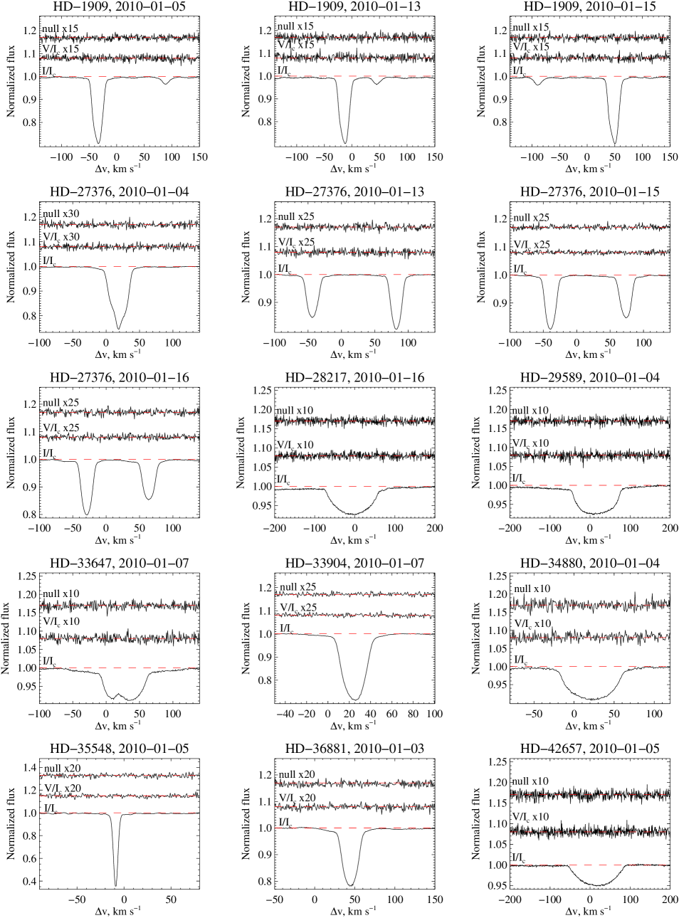
Figure 5: From bottom to top each panel shows the LSD profiles of Stokes I, V and null spectrum (if available) for all HgMn stars in our survey.

A complete summary of our analysis of the circular polarization spectra of HgMn stars is presented in Table 2. In the columns from left to right we list the stellar HD number, designation of a binary component (A – for primary, B – for secondary and AB – for one measurement of the blended components of HD 27376). This is followed by columns containing the Julian date of observation, the signal-to-noise ratio of the observed Stokes $V$ spectrum and of the reconstructed LSD Stokes $V$ profile, the mean longitudinal magnetic field derived from the Stokes $V$ and null spectra, together with the respective uncertainties. In a few cases polarization measurements were based on 2 sub-exposures only, which did not allow us to compute the null spectrum. The uncertainties correspond to 1$\sigma$ confidence levels. The last column gives the FAP for the presence of a signal in the LSD Stokes $V$ profile. All LSD Stokes $I$, $V$ and null spectra are presented in Fig. 5 (Online material).

4 Discussion

As already mentioned, previous studies of magnetic fields in HgMn stars did not detect longitudinal fields stronger than 29–100 G, and in one particular case the limits were 6–19 G. These 1 $\sigma$ error bars are not low enough to exclude the presence of the longitudinal fields weaker than $\sim$100 G, which could result from dynamically important local magnetic field structures covering only a fraction of the stellar surface. Thus, our understanding of the magnetic characteristics of these stars was fundamentally incomplete. In order to achieve a more detailed picture of the magnetic properties of HgMn stars, we studied a large sample of such stars with the most stable and modern spectropolarimeter available.

Our analysis of the Stokes $V$ spectra showed no evidence of any polarimetric signal, setting 3$\sigma$ upper limits on the longitudinal field present of 3–30 G for the majority of the stars we observed. For one sharp-lined HgMn star we obtained an uncertainty of $\sigma_{B_{z}}<$1 G, which is better than previously achieved with a single observation of any early-type star. In addition to obtaining null results for longitudinal magnetic field measurements, we analysed the Stokes $V$ LSD profiles themselves, finding no evidence for complex polarization signatures. Thus, we conclude that mercury-manganese stars do not possess strong, but topologically complex, magnetic fields. If we restrict ourselves to a dipolar magnetic field topologies, the dipole strength can be roughly estimated as $B_{\mathrm{d}}\sim 3$ $\langle B_{\mathrm{z}}\rangle$. Based on our longitudinal field measurements, we conclude that the HgMn stars do not possess dipolar fields stronger than 3–30 G.

It is important to evaluate our results in the context of the possible role of magnetic fields in the recently discovered spot formation on HgMn stars. Although there are no detailed models describing the process of the interaction between magnetic fields and the plasma, it is understood (e.g., Wade et al., 2006; Aurière et al., 2007) that this interaction becomes important when the strength of magnetic field exceeds the equipartition limit, defined by Wade et al. (2006) as $B_{\mathrm{eq}}=\sqrt{12\pi P_{\mathrm{gas}}}$. At this field strength the energy of the magnetic field equals that of the gas.

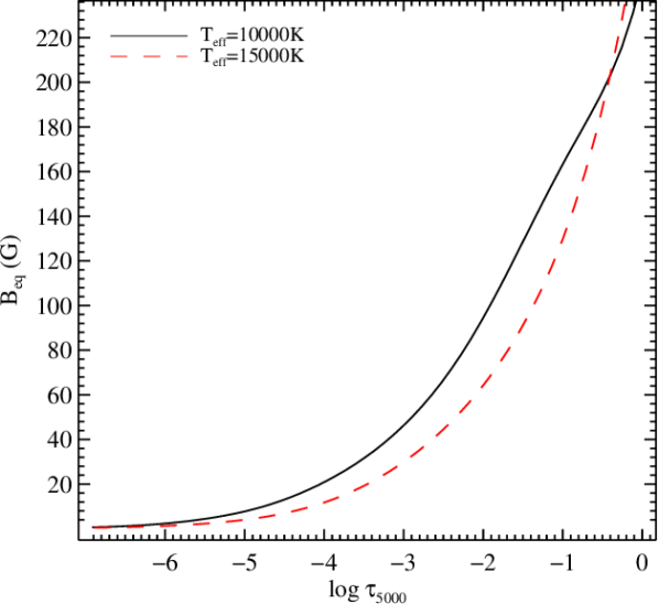
Figure 4: The equipartition magnetic field as a function of the optical depth. The solid line corresponds to the cooler model and the dashed one to the hotter.

We estimated the value of the equipartition magnetic field strength for atmosphere models with effective temperatures of $T_{\mathrm{eff}}$=10000 K and $T_{\mathrm{eff}}$=15000 K, representing the range covered by our sample of HgMn stars. Using thermodynamic parameters tabulated in these models and assuming the ideal gas law, we calculated the equipartition field as a function of the optical depth in the continuum. The result is presented in Fig. 4. From this figure we can see that the value of $B_{\mathrm{eq}}$ at $\log\tau_{5000}=-0.5$ is $\sim$200 G for the stars of both low and high effective temperatures. The value of $B_{\mathrm{eq}}$ then decreases to 100 G at $\log\tau_{5000}=-2$ for $T_{\mathrm{eff}}=$10000 K and to 60 G for $T_{\mathrm{eff}}=$15000 K. The majority of spectral lines used in our measurements form over a range in optical depth from $\log\tau_{5000}=-0.5$ to $-2$. In this interval the values of $B_{\mathrm{eq}}$ are much higher than our upper limits for the organized magnetic field on the stellar surface. Thus, it appears there are no magnetic fields on the surfaces of HgMn stars that could lead to the formation of chemical spots. These conclusions apply to the fields stronger than $\sim$ 10 G probed by our study. On the other hand, we cannot exclude the presence of complex magnetic fields with a field strength of $\sim$ 1 G in surface spots, similar to the tangled magnetic topology suggested for Vega (Petit et al., 2010).

These results lead to the conclusion that there exists a real dichotomy between HgMn and magnetic Ap stars. The latter show chemical inhomogeneities in the presence of dipolar-like magnetic fields stronger than 300 G. This limit is determined by the field strength that can withstand shearing by differential rotation and survive at the surfaces of early-type stars (Aurière et al., 2007). In contrast to magnetic Ap stars and despite a similarity in fundamental parameters, HgMn stars clearly do not have magnetic fields reaching this limit. Consequently, the surface chemical structures in mercury-manganese stars must form under a mechanism fundamentally different from magnetically-driven spot formation in hot Ap or cool active stars.

A detailed Doppler imaging study of the surface structures on the brightest HgMn star, $\alpha$ And, carried out by Kochukhov et al. (2007) using observations collected over a period of seven years led to the remarkable discovery of Hg spot evolution. This is very different from the spotted early-type magnetic stars, in which the morphology of spots remains steady over tens of years. The fact that no magnetic field was detected in $\alpha$ And (Wade et al., 2006) makes the explanation of the spot formation and evolution a very challenging task. Kochukhov et al. (2007) suggested that mercury atoms are concentrated in a thin layer where the radiation pressure and gravitational force compensate for each other. The observed changes in the spot morphology are then ascribed to hydrodynamical instabilities, upsetting the fine force balance in the Hg cloud. The physics of this intricate process and its relation to the binarity, stellar rotation and dynamic atomic diffusion effects is yet to be explored.

Despite being frequent targets of detailed abundance analyses during more than half a century, HgMn stars were recognized as spotted variables only recently. To date, 7 spotted HgMn stars have been found. It is uncertain how many more such stars will be discovered. Prior to the formulation of exotic theories of non-magnetic chemical spot formation, it is important to determine a complete picture of the occurrence rate of chemical inhomogeneities on the surface of HgMn stars. If spots are found in only a small fraction of these objects, it may be that the observed structure formation is associated with a certain stage of stellar evolution or a certain configuration of the binary system. On the other hand, discovery of spots in the majority of HgMn stars would indicate the presence of a universal hydrodynamical process, not anticipated in current stellar models.

We believe that in-depth studies of selected spotted HgMn stars as well as a broad search for spectral line variability in all accessible objects of this type will provide sufficient observational constraints for the development of a theory of non-magnetic spot formation. Analysis of known spotted stars can yield information on the time-scales of spot evolution and, possibly, on the heights of these inhomogeneities relative to the typical line formation regions. It is also important to continue searching for weak magnetic fields in spotted HgMn stars as previously done by Wade et al. (2006) for $\alpha$ And and by Folsom et al. (2010) for AR Aur. On the other hand, a line profile variability survey of a large sample of HgMn stars will help us to uncover dependencies on stellar parameters, rotation rate or binarity, possibly revealing a correlation of one these factors with the presence of spots. In subsequent studies of HgMn stars we plan to carry out both detailed studies of individual objects and to perform variability surveys to find new spectrum variable stars.

5

5

Figure 6: Continued.

5

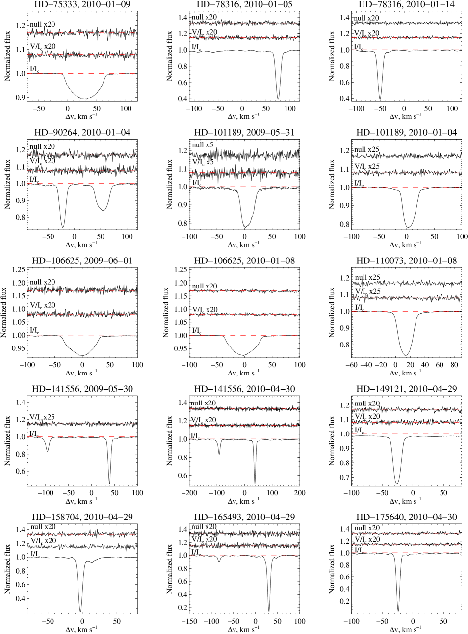
Figure 7: Continued.

5

Figure 8: Continued.