Two experiments for the price of one?
The role of the second oscillation maximum in long baseline neutrino experiments

Abstract

We investigate the quantitative impact that data from the second oscillation maximum has on the performance of wide band beam neutrino oscillation experiments. We present results for the physics sensitivities to standard three flavor oscillation, as well as results for the sensitivity to non-standard interactions. The quantitative study is performed using an experimental setup similar to the Fermilab to DUSEL Long Baseline Neutrino Experiment (LBNE). We find that, with the single exception of sensitivity to the mass hierarchy, the second maximum plays only a marginal role due to the experimental difficulties to obtain a statistically significant and sufficiently background-free event sample at low energies. This conclusion is valid for both water Čerenkov and liquid argon detectors. Moreover, we confirm that non-standard neutrino interactions are very hard to distinguish experimentally from standard three-flavor effects and can lead to a considerable loss of sensitivity to $\theta_{13}$, the mass hierarchy and CP violation.

I Introduction

Neutrino physics has seen a spectacular transition from a collection of anomalies to a field of precision study with a firmly established theoretical underpinning. All neutrino flavor transition data, with the exception of LSND Aguilar et al. (2001); *Athanassopoulos:1997er; *Athanassopoulos:1995iw; *Athanassopoulos:1997er and MiniBooNE Aguilar-Arevalo et al. (2007); *AguilarArevalo:2008rc; *AguilarArevalo:2010wv, can be described by oscillation of three active neutrino flavors, see e.g. the reviews in Gonzalez-Garcia and Maltoni (2008); Maltoni et al. (2004). Throughout this paper we assume that LSND and MiniBooNE have explanations which do not affect our results, i.e. they are not due to neutrino oscillation.

Within the three flavor oscillation framework, experiments have determined the values of the mass squared differences and the associated large mixing angles with a precision at the level of a few percent Maltoni et al. (2004). Currently unknown are the size of $\theta_{13}$, the value of the CP phase $\delta_{\mathrm{CP}}$ and the sign of the atmospheric mass splitting $\Delta m^{2}_{31}$, as well whether $\theta_{23}$ is exactly $\pi/4$, and if not, whether it is larger or smaller than $\pi/4$. The ultimate goal is to determine the neutrino mixing matrix with at least the same level of precision and redundancy as the CKM matrix in the quark sector. The size of $\theta_{13}$ plays a particularly crucial role, since this quantity will set the scale for the effort necessary to answer the open questions. The need to determine $\theta_{13}$ has spurred a number of reactor neutrino experiments Anderson et al. (2004) using disappearance of $\bar{\nu}_{e}$: Double Chooz Ardellier et al. (2004), RENO Ahn et al. (2010) and Daya Bay Guo et al. (2007). Their discovery reach at $3\,\sigma$ confidence level will go down to approximately $\sin^{2}2\theta_{13}=10^{-2}$ Huber et al. (2009); Mezzetto and Schwetz (2010). At the same time the next generation of long baseline experiments looking for $\nu_{\mu}\rightarrow\nu_{e}$ is underway with T2K Itow et al. (2001) and NO$\nu$A Ayres et al. (2004). Neither T2K nor NO$\nu$A can provide information on $\delta_{\mathrm{CP}}$ beyond a mere indication and even that is only possible in combination with the data from Daya Bay Huber et al. (2009). The discovery of the mass hierarchy, if discovery is defined at the usual $5\,\sigma$ confidence level, will not be possible; even a $3\,\sigma$ evidence is very unlikely Huber et al. (2009). Therefore, it has been widely recognized that long baseline experiments with physics capabilities far beyond NO$\nu$A and T2K are necessary, for a review of the possibilities, see reference Bandyopadhyay et al. (2007).

Here, we would like to focus on the superbeam concept, or more specifically on what is called a wide band beam (WBB). In a superbeam, muon neutrinos are produced by the decay of pions, where the pions have been produced by proton irradiation of a solid target. All neutrino beams relevant in the context of this study use a magnetic horn to focus and sign-select the pions. In a wide band beam, the detector is on-axis and thus receives a wide (sic!) energy spectrum of neutrinos. The wide band beam concept makes maximal use of the available pions and thus provides higher event rates compared to a narrow band or off-axis beam. The price to pay for the wide spectrum is that the detector needs to have a very good energy resolution, and the existence of a high energy tail in the beam will lead to feed down of neutral current background events. Thus, a wide band beam imposes unique demands on the detector technology. Apart from allowing for more events, the wide beam spectrum allows to study a range of $L/E$ values within one experiment, and possibly even to observe more than only one oscillation maximum. On the level of oscillation probabilities, the ability to observe two or more cycles of the oscillation obviously allows to distinguish between otherwise degenerate solutions. Therefore, the observation of the second oscillation maximum is considered to play an important role in wide band beam experiments. The purpose of the present paper is to study in detail and in a quantitative manner whether the assertion of the role of the second oscillation maximum based on probabilities remains valid in a full numerical sensitivity calculation. We also include the case of non-standard interactions, where one expects similar benefits from the presence of the second oscillation maximum.

In order to perform a full numerical sensitivity calculation we need to specify the experimental parameters in great detail and therefore have to constrain the numerical analysis to a specific setup, which we model to resemble the Fermilab to DUSEL Long Baseline Neutrino Experiment (LBNE). However, whenever the specifics of the chosen experimental setup obscure the underlying physics, we will show results for sensible variations around our chosen setup. In section II we discuss the theoretical framework with respect to standard and non-standard oscillations. In section III we spell out the details of the experimental setup and describe our analysis techniques. Section IV will contain our results on both three flavor oscillation and non-standard interactions and finally in section V we will summarize our findings and present our conclusion. In appendix A we show supplementary results on variations of the total exposure and baseline.

II Framework

II.1 Three flavor oscillation

In this paper our main concern is the measurement of the transition probabilities $P(\nu_{\mu}\rightarrow\nu_{e})$ and $P(\bar{\nu}_{\mu}\rightarrow\bar{\nu}_{e})$. Since the baseline considered is longer than $1,000\,\mathrm{km}$, matter effects will play an important role. While the underlying Hamiltonian describing oscillations in the presence of a matter potential is quite simple, the resulting expressions for the exact oscillation probabilities are not. Therefore, a plethora of approximations have been devised, for an overview see reference Akhmedov et al. (2004). Even these approximate solutions have a very rich structure; in particular, for fixed energy, any given value of the oscillation probability can typically be realized by different combinations of oscillation parameters. The possible degenerate solutions can be classified into the intrinsic ambiguity Burguet-Castell et al. (2001), the sign of $\Delta m^{2}_{31}$ ambiguity Minakata and Nunokawa (2001) and the octant ambiguity Fogli et al. (1997). Combined, these three ambiguities give rise to what has become known as the eightfold degeneracy Barger et al. (2002). A recent comprehensive analytical discussion of the eightfold degeneracy can be found in reference Minakata and Uchinami (2010). In the context of long baseline experiments the most worrisome degeneracy stems from a combination of the intrinsic and sign ambiguity which can lead to a phenomenon called $\pi$-transit Huber et al. (2002), in which a CP violating true solution is mapped into a CP conserving fake solution. A large number of possible remedies has been proposed in the literature, here we focus on the proposal to use not only neutrino and anti-neutrino events from the 1^st oscillation maximum, but also from the 2^nd oscillation maximum.

In figure 1 we illustrate how the use of the 2^nd oscillation maximum can alleviate the sign degeneracy. At a baseline of $1,300\,\mathrm{km}$, the first oscillation maximum occurs with $\Delta m_{31}^{2}=2.4\times 10^{-3}\,\mathrm{eV}^{2}$ for $E_{\nu}=2.5\,\mathrm{GeV}$ and the second oscillation maximum is at $E_{\nu}=0.84\,\mathrm{GeV}$. The first zero of the oscillation term occurs at $E_{\nu}=1.25\,\mathrm{GeV}$, and we will use this energy to separate events from the two oscillation maxima, assigning all events below to the second maximum and all above to the first. In figure 1 we show so called bi-rate plots. In a bi-rate plot $\theta_{13}$ is kept fixed and the coordinates are the total number of events in the neutrino channel and in the anti-neutrino channel, respectively. For each possible choice of the CP phase one obtains a point in this kind of diagram, and as the CP phase is continuously varied from $-\pi$ to $+\pi$ the points trace out a banana-shaped curve (or, on a linear scale, an ellipse) Winter (2004). This is similar to a bi-probability plot Minakata and Nunokawa (2001), but avoids the problem of choosing a neutrino energy for plotting and thus allows a closer approximation of the experimental realities. In figure 1, we moreover separated the event sample into events below $1.25\,\mathrm{GeV}$ (green/light gray curves) and events above that energy (blue/dark gray curves). The solid lines are for normal hierarchy and the dashed ones for inverted. The solid disks indicate the event rates for $\delta_{\mathrm{CP}}=-\pi/2$, whereas the open circles indicate the event rates for $\delta_{\mathrm{CP}}=+\pi/2$. Focusing on the $2^{\mathrm{nd}}$ maximum (green/light gray lines), we see that the “bananas” for both hierarchies are very similar and occupy essentially the same area in the event rate plane. Moreover, the event rates at the two maximally CP violating values of $\delta_{\mathrm{CP}}=\pm\pi/2$ do not change when going from one hierarchy to the other. For the $1^{\mathrm{st}}$ maximum (blue/dark gray lines), the two “bananas” are very different and the event rates for the same value of $\delta_{\mathrm{CP}}$ change greatly when switching the hierarchy. Therefore, given enough statistics, we expect the measurement in the $2^{\mathrm{nd}}$ maximum to provide a clean value for $\delta_{\mathrm{CP}}$, but no information on the hierarchy. The measurement in the $1^{\mathrm{st}}$ maximum, on the other hand, should yield strong evidence for the mass hierarchy, but may suffer from degeneracies for the determination of $\delta_{\mathrm{CP}}$. The combination of the two maxima should result in a clear and unambiguous determination of both the mass hierarchy and the CP phase.

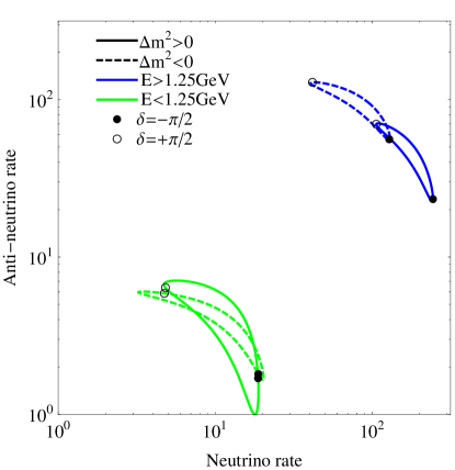
Figure 1: Bi-rate plot for a typical wide band beam for the 1^st (blue/dark gray) and 2^nd (green/light gray) oscillation maximum for normal (solid) and inverted (dashed) hierarchy. Along each of the banana-shaped curves, the CP phase $\delta_{\mathrm{CP}}$ varies from $-\pi$ to $\pi$, where $\delta_{\mathrm{CP}}=-\pi/2$ is denoted by a solid disk and $\delta_{\mathrm{CP}}=+\pi/2$ by an open circle. We have assumed $\sin^{2}2\theta_{13}=0.025$, and the other oscillation parameters are chosen according to eq. (III.2).

II.2 Non-standard Interactions

At energies of a few GeV, relevant to accelerator neutrino oscillation experiments, the effects of new physics, which is expected at or above the electroweak scale, can be parametrized in terms of an effective theory. Some types of low-scale new physics can also be parametrized that way Joshipura and Mohanty (2004); Nelson and Walsh (2008). A well known example for the use of effective theory is the Fermi theory of nuclear beta decay. In this paper, we will use such non-standard neutrino interactions (NSI) as a benchmark scenario for deviations from the standard three-flavor oscillation framework, but we should keep in mind that new physics in the neutrino sector can also have different manifestations; examples are CPT violation or mixing between active and sterile neutrinos. Typical operators inducing non-standard neutrino interactions (NSI) are

$$\mathcal{L}_{\rm CC} \supset-2\sqrt{2}G_{F}\varepsilon^{{\rm CC},f,f^{\prime}}_{\alpha\beta}\left[\bar{\nu}_{\alpha}\gamma^{\rho}P_{L}\ell_{\beta}\right]\left[\bar{f}\gamma_{\rho}P_{L}f^{\prime}\right]+{\rm h.c.}$$ (1)

(charged current NSI) and

$$\mathcal{L}_{\rm NC} \supset-2\sqrt{2}G_{F}\varepsilon^{{\rm NC},f}_{\alpha\beta}\left[\bar{\nu}_{\alpha}\gamma^{\rho}P_{L}\nu_{\beta}\right]\left[\bar{f}\gamma_{\rho}P_{L}f\right]+{\rm h.c.}\,.$$ (2)

(neutral current NSI). Here, $G_{F}=\sqrt{2}g^{2}/8M_{W}^{2}$ is the Fermi constant, $P_{L}=(1-\gamma^{5})/2$, $\alpha$ and $\beta$ are flavor indices of the neutrinos $\nu$ and the charged leptons $\ell$, and the fermions $f$ and $f^{\prime}$ are the members of an arbitrary weak doublet. The parameters $\varepsilon^{{\rm CC},f,f^{\prime}}_{\alpha\beta}$ and $\varepsilon^{{\rm NC},f}_{\alpha\beta}$ give the relative magnitude of the NSI compared to standard weak interactions. For new physics around the TeV scale, we expect their absolute values to be of order $10^{-3}$–$10^{-2}$. In the presence of new degrees of freedom below the electroweak scale, NSI could be larger and also expectations for the magnitude of NSI based on effective theory approaches Gavela et al. (2009); Antusch et al. (2009) may be too conservative. Note that equations 1 and 2 include only $V-A$ type interactions, but in principle, more general Lorentz structures are possible (see e.g. refs. Kopp et al. (2008); Kopp (2009) for an overview).

For phenomenological purposes, it is convenient to parametrize NSI in a slightly different way. Consider the $\nu_{\alpha}\to\nu_{\beta}$ oscillation probability at baseline $L$,

$$P_{\alpha\beta}=|\langle\nu_{\beta}|e^{-iHL}|\nu_{\alpha}\rangle|^{2}\,,$$ (3)

with the Hamiltonian

$$H =U\begin{pmatrix}0&&\\ &\Delta m_{21}^{2}/2E&\\ &&\Delta m_{31}^{2}/2E\end{pmatrix}U^{\dagger}+V_{\rm MSW}\,,$$ (4)

where $U$ is the leptonic mixing matrix, $E$ is the neutrino energy, and $V_{\rm MSW}$ is the $3\times 3$ matrix describing matter effects. In the presence of CC NSI, the initial and final states get modified according to

$$|\nu^{s}_{\alpha}\rangle=|\nu_{\alpha}\rangle+\sum_{\beta=e,\mu,\tau}\varepsilon^{s}_{\alpha\beta}|\nu_{\beta}\rangle\quad\text{and}\quad\langle\nu^{d}_{\beta}|=\langle\nu_{\beta}|+\sum_{\alpha=e,\mu,\tau}\varepsilon^{d}_{\alpha\beta}\langle\nu_{\alpha}|\,,$$ (5)

respectively. The parameters $\varepsilon^{s}_{\alpha\beta}$ and $\varepsilon^{d}_{\alpha\beta}$, which are closely related to the parameters $\varepsilon^{{\rm CC},f,f^{\prime}}_{\alpha\beta}$ defined above Kopp et al. (2008); Kopp (2009), describe non-standard admixtures to the neutrino states produced in association with a charged lepton of flavor $\alpha$ or detected in a process involving a charged lepton of flavor $\beta$, respectively. Note that in $\varepsilon^{s}_{\alpha\beta}$, the first index corresponds to the flavor of the charged lepton, and the second one to that of the neutrino, while in $\varepsilon^{d}_{\alpha\beta}$, the order is reversed. The matrices $(1+\varepsilon^{s})$ and $(1+\varepsilon^{d})$ need not be unitary, i.e. $|\nu^{s}_{\alpha}\rangle$ and $|\nu^{d}_{\alpha}\rangle$ are not required to form complete orthonormal sets of basis vectors in the Hilbert space. Instead of considering an oscillation probability $P$ normalized to unity, it is therefore more useful to consider the apparent oscillation probability $\tilde{P}(\nu^{s}_{\alpha}\to\nu^{d}_{\beta})$, defined as the number of neutrinos produced together with a charged lepton of flavor $\alpha$ and converting into a charged lepton of flavor $\beta$ in the detector, divided by the same number in the absence of oscillations and non-standard interactions. The apparent oscillation probability is given by

$$\tilde{P}(\nu^{s}_{\alpha}\to\nu^{d}_{\beta}) =|\langle\nu^{d}_{\beta}|e^{-i\tilde{H}L}|\nu^{s}_{\alpha}\rangle|^{2}$$

$$=\big{|}(1+\varepsilon^{d})_{\gamma\beta}\,\big{(}e^{-i\tilde{H}L}\big{)}_{\gamma\delta}(1+\varepsilon^{s})_{\alpha\delta}\big{|}^{2}$$

$$=\Big{|}\Big{[}\big{(}1+\varepsilon^{d}\big{)}^{T}\,\,e^{-i\tilde{H}L}\,\,\big{(}1+\varepsilon^{s}\big{)}^{T}\Big{]}_{\beta\alpha}\Big{|}^{2}\,,$$ (6)

where $\tilde{H}=U\,{\rm diag}(0,\Delta m_{21}^{2}/2E,\Delta m_{31}^{2}/2E)\,U^{\dagger}+\tilde{V}_{\rm MSW}$. The modified matter potential is

$$\tilde{V}_{\rm MSW}=\sqrt{2}G_{F}N_{e}\begin{pmatrix}1+\varepsilon^{m}_{ee}&\varepsilon^{m}_{e\mu}&\varepsilon^{m}_{e\tau}\\ \varepsilon^{m*}_{e\mu}&\varepsilon^{m}_{\mu\mu}&\varepsilon^{m}_{\mu\tau}\\ \varepsilon^{m*}_{e\tau}&\varepsilon^{m*}_{\mu\tau}&\varepsilon^{m}_{\tau\tau}\end{pmatrix}\,,$$ (7)

with $\varepsilon^{m}_{\alpha\beta}$ being closely related to the $\varepsilon^{{\rm NC},f}_{\alpha\beta}$ from equation 2. As explained above, the magnitude of the $\varepsilon^{s,d,m}$ parameters is expected to be at or below the $10^{-2}$ level for new physics at the TeV scale.

Model-independent experimental bounds on the $\varepsilon^{s,d,m}$ parameters are typically of $\mathcal{O}(10^{-2}-1)$ Davidson et al. (2003); Gonzalez-Garcia and Maltoni (2008); Biggio et al. (2009). In a specific model, however, the bounds may be much stronger because in most models neutrino NSI are accompanied by charged lepton flavor violation, which is strongly constrained by precision tests of the electroweak theory and by rare decay searches. From a model building point of view, it is therefore not easy to realize large non-standard neutrino interactions that can saturate the experimental bounds Gavela et al. (2009); Antusch et al. (2009).

Obviously, with any new experiment, we need to compare the expected bounds on new physics with the ones we already have. We use the bounds derived in Davidson et al. (2003); Gonzalez-Garcia and Maltoni (2008); Biggio et al. (2009) as our benchmark. In particular, we use the 90% confidence level constraints $|\varepsilon^{m}_{ee}|<4.2$, $|\varepsilon^{m}_{e\mu}|<0.33$, $|\varepsilon^{m}_{e\tau}|<3.0$ $|\varepsilon^{m}_{\mu\mu}|<0.068$, $|\varepsilon^{m}_{\mu\tau}|<0.063$, $|\varepsilon^{m}_{\tau\tau}|<0.2$. Note that the relatively strong constraints on $|\varepsilon^{m}_{\mu\tau}|$ and $|\varepsilon^{m}_{\tau\tau}|$ have been derived from atmospheric neutrino data in a two-flavor framework; when three-flavor effects—in particular correlations between different types of NSI—are taken into account, these bounds may become somewhat weaker Blennow et al. (2008); Friedland and Lunardini (2005).

III Methods

III.1 Experimental setup

To assess the sensitivity of a wide band neutrino beam to standard and non-standard oscillation physics, we have performed simulations using the GLoBES software Huber et al. (2005, 2007), with an implementation of NSI developed in refs. Kopp et al. (2007, 2008); Kopp (2008). Our experiment description follows the LBNE proposal for a long-baseline neutrino beam from Fermilab to DUSEL, but our results will hold qualitatively also for other wide band beam experiments.

III.1.1 Beam

For the neutrino beam, we consider the options listed in table 1. We use the unit protons on target (pot) since it is the usual measure of integrated luminosity, $\mathcal{L}$, for this kind of experiments. To compare this with other beams of different energy it is useful to convert this result to equivalent beam power, $P$, where we assume that the beam is on for $2\times 10^{7}\,\mathrm{s}$ per tropical year.

$$P=0.801\,\left(\frac{E_{p}}{\mathrm{GeV}}\right)\left(\frac{\mathcal{L}}{10^{20}\,\text{pot per year}}\right)\,\mathrm{kW}\,.$$

With this in mind, the luminosities given in table 1 correspond to about 6 years of running (3 years in neutrino mode + 3 years in anti-neutrino mode) at a beam power of either $\sim 700\,\mathrm{kW}$ or $\sim 2,300\,\mathrm{kW}$. We have also studied the performance of a $60\,\mathrm{GeV}$ beam, which would have the advantage of lower backgrounds, at the expense of less statistics. Since we found only very minor performance differences between the $60\,\mathrm{GeV}$ and $120\,\mathrm{GeV}$ options, we restrict the discussion to the $120\,\mathrm{GeV}$ beam in the following. Simulated spectra for all beam options have been kindly provided to us by the LBNE collaboration Bishai (2010).

Proton energy	pot per polarity	Comment
120 GeV	$22\times 10^{20}$	accelerator complex without Project X
120 GeV	$72\times 10^{20}$	accelerator complex with Project X

Table 1: Neutrino beam configurations considered in our simulations.

III.1.2 Detectors

We assume the far detector to be located at a baseline $L=1,300\,\mathrm{km}$, corresponding to the distance from Fermilab to DUSEL, which translates into an energy $E\sim 2.5\,\mathrm{GeV}$ for the 1^st oscillation maximum. In order to be sensitive to both oscillation maxima, and given the beam spectra, the detector needs to have good efficiency in the energy range from $0.5-4\,\mathrm{GeV}$. The number of events in the 1^st oscillation maximum will be significantly larger than that in the 2^nd maximum. Currently, two detector technologies are considered in this context

1. A water Čerenkov (WC) detector with a fiducial mass of $200\,\mathrm{kt}$. As demonstrated by Super-Kamiokande, this type of detector allows for a clean separation of muon and electron quasi-elastic events. However, its application at GeV energies requires careful consideration of possible backgrounds from neutral current events giving rise to energetic neutral pions. A considerable amount of work went into studying this issue Yanagisawa et al. (2007); Dufour et al. (2010). Both studies agree quite well and we use the results from reference Yanagisawa et al. (2007). The GLoBES description of this WC detector is based on references Barger et al. (2006); Diwan et al. (2006). This simulation includes energy-dependent efficiency tables, smearing matrices, and background estimates based on Monte-Carlo codes developed by the Super-Kamiokande collaboration Yanagisawa et al. (2007). We include both events from the $\nu_{e}$ appearance channel as well as the $\nu_{\mu}$ disappearance channel, for both neutrino and anti-neutrino running.

2. A liquid argon (LAr) time projection chamber (TPC) with a fiducial mass of $34\,\mathrm{kt}$. For the case of LAr, only much less detailed and accurate simulations are available since no large LAr detector has ever been operated. The LAr description is based on references Fleming and Zeller (2008); Barger et al. (2007). We include the $\nu_{e}$ and $\bar{\nu}_{e}$ appearance channels, with backgrounds from the intrinsic $\nu_{e}$/$\bar{\nu}_{e}$ contamination of the beam, misidentified muons, and neutral current events. Our background estimate is conservative because the very high spatial resolution and the ability to detect very low energy particles in a LAr detector might allow for a much more efficient rejection of neutral current events. For the $\nu_{\mu}$ ($\bar{\nu}_{\mu}$) disappearance channel, the main backgrounds stem from neutral current events (we assume a rejection efficiency of 99.5%) and from the $\bar{\nu}_{\mu}$ ($\nu_{\mu}$) “wrong sign” contamination of the beam. Since the oscillation probabilities in the $\nu_{\mu}$ and $\bar{\nu}_{\mu}$ disappearance channels are similar (except for the sub-leading contribution from matter effects), the latter background does not constitute a problem.

For both detectors, the neutrino cross sections are based on Messier (1999); Paschos and Yu (2002); they are computed for water and isoscalar targets, respectively. In an actual experiment great care needs to be taken to correctly model the cross sections, including nuclear effects. In our case, since we are using the same cross section to compute the data and perform the fit to that simulated data, any error due to the omission of nuclear effects will cancel.

In our simulations we also include a near detector; for standard oscillation physics, its main effect is to reduce systematic uncertainties in the far detector, but for charged current NSI searches, it is valuable also as a standalone detector and its inclusion in the simulation is imperative. Since no specific technology has been chosen for the LBNE near detector(s) yet, we take a generic approach and assume the near detector to have identical properties (resolution, efficiencies, backgrounds, etc.) as the far detector, but a fiducial mass of only 1 kt. Furthermore, we assume the geometric acceptance of the near and far detectors to be the same, which greatly simplifies the calculation, but is very difficult to achieve in practice. In reality, the optimum choice of near detector technology and geometry may be very different for the WC and LAr cases, and thus also the effective systematic uncertainties may be quite different.

For illustration, we show in fig. 2 the expected event rates in the $\nu_{e}$ appearance channel for both detectors. It is clear that for small $\theta_{13}$, backgrounds will be a limitation. In particular, neutral current events contaminate the second oscillation peak.

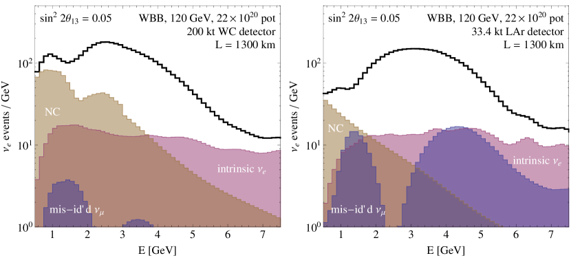
Figure 2: Expected event rates in the $\nu_{e}$ appearance channel for $\sin^{2}2\theta_{13}=0.05$, $\delta_{\mathrm{CP}}=0$ as a function of the reconstructed neutrino energy. The black histograms show the signal + background rates, while the filled red, blue, and beige histograms depict the backgrounds due to the intrinsic $\nu_{e}$ contamination of the beam, misidentified $\nu_{\mu}$ events, and neutral current events, respectively. Except for $\theta_{13}$ and $\delta_{\mathrm{CP}}$, the oscillation parameters are chosen according to eq. (III.2).

III.2 Analysis

To analyze the simulated data sets and to compute exclusion limits and allowed parameter regions, we use a $\chi^{2}$ analysis following ref. Huber et al. (2002). Our $\chi^{2}$ function has the form

$$\chi^{2}=\min_{\vec{a}}\Big{[}\,\sum_{d=N,F}\;\sum_{s=\nu_{e},\bar{\nu}_{e},\nu_{\mu},\bar{\nu}_{\mu}}\sum_{j=1}^{\#\text{ of bins}}\chi^{2}_{\rm stat}\Big{(}N^{\rm obs}_{d,s,j},N^{\rm th}_{d,s,j}(\vec{\Theta}),\vec{a}\Big{)}+\sum_{i}\frac{a_{i}^{2}}{(\sigma^{a}_{i})^{2}}\Big{]}+\sum_{j}\frac{(\Theta_{j}-\Theta^{(0)}_{j})^{2}}{(\sigma^{\Theta}_{j})^{2}}\,,$$ (8)

where $N^{\rm obs}_{d,s,j}$ and $N^{\rm th}_{d,s,j}(\vec{\Theta})$ are the observed and theoretically predicted event rates for detector $d$ ($d=N$ (near) or $F$ (far)), event sample $s$ ($s=\nu_{e},\bar{\nu}_{e},\nu_{\mu},\bar{\nu}_{\mu}$), and bin $j$. The vector $\vec{\Theta}$ stands for the oscillation parameters, while $\vec{a}$ contains the systematical biases. The first term on the right hand side of equation 8 is the statistical contribution to $\chi^{2}$, while the second term contains pull terms that disfavor values of the biases $a_{i}$ much larger than the associated systematic uncertainties $\sigma^{a}_{i}$. In a similar way, the last term of equation 8 is used to confine the oscillation parameters to within the region determined by other experiments, where, for each oscillation parameter $\Theta_{j}$, $\Theta^{(0)}_{j}$ denotes the externally given best fit value and $\sigma^{\Theta}_{j}$ the $1\sigma$ uncertainty on that value. In our simulations, we include such external prior terms only for the solar oscillation parameters $\theta_{12}$ and $\Delta m_{21}^{2}$ to which the wide band beam is not sensitive. We assume the solar parameters to be known to within 5% at the $1\sigma$ level, while for all other oscillation parameters, we set $\sigma^{\Theta}_{j}=\infty$. The default oscillation parameters used in this study are, in agreement with current fits Maltoni et al. (2004),

$$\sin^{2}\theta_{12}=0.32\,, \theta_{13}=0\,,$$

$$\theta_{23}=\frac{\pi}{4}\,, \delta_{\mathrm{CP}}=\frac{3}{2}\pi\,,$$

$$\Delta m^{2}_{21}=+7.6\times 10^{-5}\,\mathrm{eV}^{2}\,, \Delta m^{2}_{31}=+2.4\times 10^{-3}\,\mathrm{eV}^{2}\,,$$ (9)

and we use a conservative 5% uncertainty on the matter density.

The systematic errors we include in our study are listed in Table 2 for both detector technologies. We treat the normalization of the beam flux and of the background contributions to the $\nu_{e}$ and $\bar{\nu}_{e}$ event samples as completely free parameters, i.e. we do not include pull terms for them. Moreover, we allow for uncorrelated systematic biases in the number of signal and background events in each event sample and each detector. Systematic uncertainties are assumed to be completely uncorrelated between the neutrino and anti-neutrino runs of the experiment.

	WC	LAr	N/F correlated?
Beam flux [%]	$\infty$	$\infty$	yes
Intrinsic background [%]	$\infty$	$\infty$	yes
Signal normalization for $\nu_{e}$ sample [%]	0.7	0.7	no
Background normalization for $\nu_{e}$ sample [%]	3.5	7.0	no
Signal normalization for $\nu_{\mu}$ sample [%]	0.7	3.5	no
Background normalization for $\nu_{\mu}$ sample [%]	7.0	7.0	no

Table 2: Systematic uncertainties assumed in our simulations. All systematic errors are assumed to be completely uncorrelated between the neutrino and anti-neutrino runs of the experiment. Note that uncertainties that are uncorrelated between the near (N) and far (F) detectors will add in quadrature when translated into an error on the measured oscillation probability. For example the near-far uncorrelated 0.7% uncertainty in the number of $\nu_{e}$ signal events would translate into a 1% uncertainty on the measured oscillation probability.

We use the following performance indicators to estimate the sensitivity of the experiment to standard oscillation physics

• $\theta_{13}$ discovery reach. For each combination of true $\theta_{13}$ and true $\delta_{\mathrm{CP}}$, we compute the expected experimental event rates, and then perform a $\chi^{2}$ fit assuming a test value of $\theta_{13}=0$. If, for a particular combination of $\theta_{13}^{\rm true}$ and $\delta_{\mathrm{CP}}^{\rm true}$, the fit disagrees with the simulated data at a given confidence level, we say that that this $\theta_{13}^{\rm true}$ and $\delta_{\mathrm{CP}}^{\rm true}$ are within the discovery reach of the experiment at that confidence level. In the fit, we marginalize over all oscillation parameters except $\theta_{13}$ (which is kept fixed at zero) as well as the matter density.

• Discovery reach for the normal mass hierarchy (NH) For each point in the $\theta_{13}^{\rm true}$–$\delta_{\mathrm{CP}}^{\rm true}$ plane, we simulate the event rates assuming a normal mass hierarchy, and then attempt a fit to the simulated data assuming the inverted hierarchy. If the fit is incompatible with the data at a given confidence level, we say that the chosen combination of $\theta_{13}^{\rm true}$ and $\delta_{\mathrm{CP}}^{\rm true}$ is within the NH discovery reach of the experiment.

• CP violation (CPV) discovery reach. For each point in the $\theta_{13}^{\rm true}$–$\delta_{\mathrm{CP}}^{\rm true}$ plane, we simulate the expected event rates and then attempt fits assuming $\delta_{\mathrm{CP}}=0$ and $\delta_{\mathrm{CP}}=\pi$. If the fits are able to exclude the CP conserving solutions at a given confidence level, we say that the chosen combination of $\theta_{13}^{\rm true}$ and $\delta_{\mathrm{CP}}^{\rm true}$ is within the CPV discovery reach of the experiment.

• Sensitivity to the octant of $\boldsymbol{\theta_{23}}$. For each point in the $\theta_{23}^{\rm true}$–$\theta_{13}^{\rm true}$ plane, we simulate the expected event rates and then attempt a fit in which all parameters are marginalized over, but $\theta_{23}$ is forced to lie in the “wrong” octant, i.e. between $\pi/4$ and $\pi/2-\theta_{23}^{\rm true}$. If the fit is incompatible with the simulated data at a given confidence level, we say that the experiment is sensitive to the octant of $\theta_{23}$ at that confidence level.

When discussing non-standard neutrino interactions, we will use the NSI discovery reach as a performance indicator, which we define in analogy to the $\theta_{13}$ discovery reach: For each set of true NSI parameters, we check whether a standard oscillation fit neglecting NSI is compatible with the data at a given confidence level. If this is not the case, the chosen NSI parameters are within the experimental discovery reach.

IV Results

IV.1 Standard oscillation

First, we summarize the physics performance of the default setup, as defined in section III.1, with respect to three flavor oscillation. Figure 3 depicts the discovery reaches for CPV, $\theta_{13}$ and the mass hierarchy. In the left hand panel we show results for a $200\,\mathrm{kt}$ water Čerenkov detector (WC), whereas in the right hand panel we show the corresponding results for a $34\,\mathrm{kt}$ liquid argon detector (LAr). We have checked that the difference in performance between the $60\,\mathrm{GeV}$ and $120\,\mathrm{GeV}$ proton beams, at equivalent power, is very small, and therefore we only show the result for the $120\,\mathrm{GeV}$ beam.

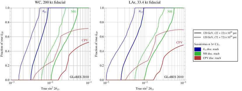
Figure 3: Sensitivity to standard oscillation physics in a wide band beam for a $200\,\mathrm{kt}$ (fiducial) water Čerenkov detector (left) and a $34\,\mathrm{kt}$ (fiducial) liquid argon detector (right). The results are shown at $3\,\sigma$ confidence level.

It is apparent from this figure that the performance of the two detectors, despite a factor of 6 difference in fiducial masses, is quite similar. If $\sin^{2}2\theta_{13}<0.04$ the beam upgrade provided by Project X, whose results are shown as dotted lines, is a necessity to ensure a mass hierarchy determination and to maintain a better than 50% coverage for CP violation. Even for the largest possible values of $\theta_{13}$ the CP sensitivity would greatly benefit from a luminosity upgrade, as also can be seen from figure 9. We have also evaluated the relative precision on $\sin^{2}2\theta_{13}$, defined by $(\sin^{2}2\theta_{13}^{\rm max}-\sin^{2}2\theta_{13}^{\rm min})/\sin^{2}2\theta_{13}^{\rm true}$, where $\theta_{13}^{\rm min}$ and $\theta_{13}^{\rm max}$ denote the lower and upper bounds on $\theta_{13}$ that can be expected for a particular $\theta_{13}^{\rm true}$. We find for $\sin^{2}2\theta_{13}^{\rm true}=0.1$ that the WC detector measures $\sin^{2}2\theta_{13}$ with a relative $3\sigma$ error between 33% and 39%, depending on the true value of $\delta_{\mathrm{CP}}$, while the LAr detector can achieve a precision between 36% and 42%. This result should be compared with the accuracy obtainable from reactor neutrino experiments like Daya Bay, which will provide a relative error of 18% at $3\sigma$ C.L. Huber et al. (2009).

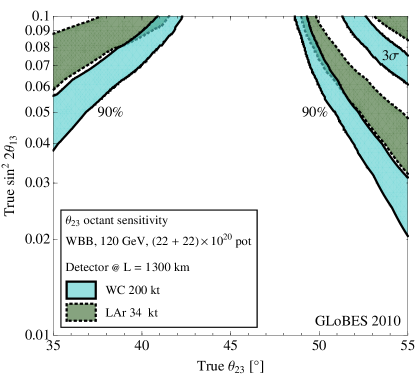
Figure 4: Ability to determine the octant of $\theta_{23}$ at $3\,\sigma$ and $90\%$ confidence level for $200\,\mathrm{kt}$ WC and and $34\,\mathrm{kt}$ LAr detectors as labeled in the legend. The result is shown as a function of $\theta_{23}^{\rm true}$ and $\sin^{2}2\theta_{13}^{\rm true}$. The width of each region is due to the unknown CP phase.

In figure 4 we study the ability to determine the octant of $\theta_{23}$ in a WC or LAr detector. The width of the colored regions in the plot is due to the marginalization over the unknown CP phase $\delta_{\mathrm{CP}}^{\rm true}$. For this measurement, we see again that the differences in performance between a WC detector and a six times smaller LAr detector are small. Determining the octant of $\theta_{23}$ is a difficult measurement for any experiment. In particular, for $\theta_{23}$ close to $45^{\circ}$ this measurement is only possible for large $\theta_{13}$. The asymmetry in sensitivity between $\theta_{23}^{\rm true}$ above or below $45^{\circ}$ is due to the partial cancellation between the octant sensitive terms in $P_{\mu e}$ and matter effects. Therefore, the sign of the asymmetry will change if we were to change the assumed true mass hierarchy from normal to inverted in our calculation.

IV.2 2^nd maximum

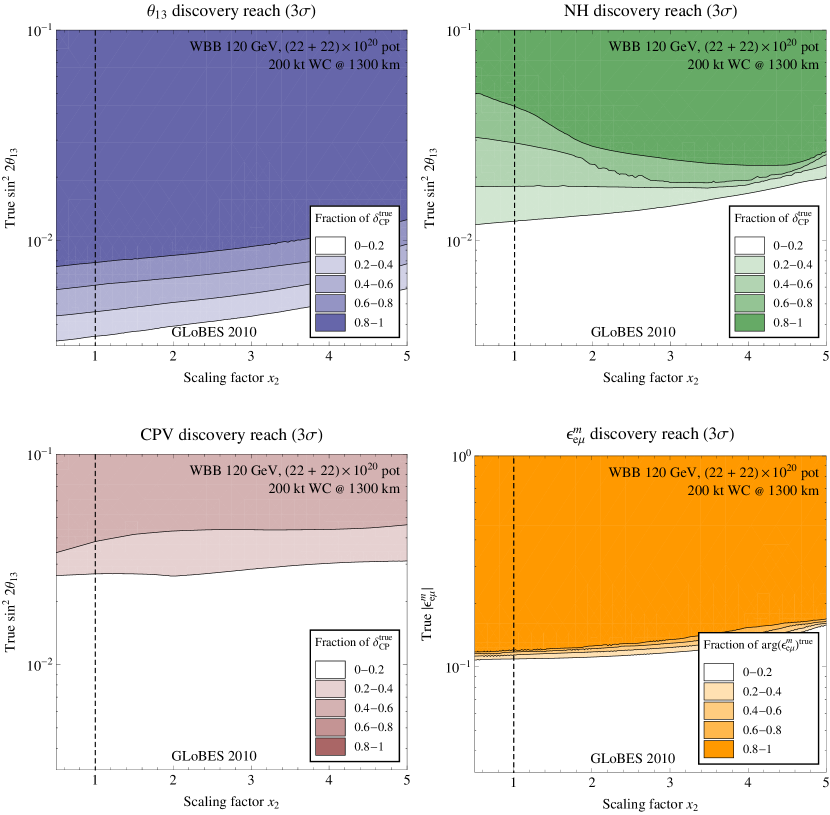
Figure 5: The dependence of various sensitivities, as labeled in the legend of each panel, on the scaling parameter $x_{2}$ as defined in equation 10. Shown are lines of constant CP fraction in the $x_{2}$–$\sin^{2}2\theta_{13}^{\rm true}$ resp. $x_{2}$–$|(\varepsilon^{m}_{e\mu})^{\rm true}|$ plane. The results are given at $3\,\sigma$ confidence level.

Now that we have established the baseline performance, we can turn our attention to the central question of this paper: what is the quantitative impact of data from the $2^{\mathrm{nd}}$ oscillation maximum on the physics sensitivities? This question specifically neglects the issue of how the robustness of an experiment with respect to unforeseen systematical effects improves due to the data from $2^{\mathrm{nd}}$ oscillation maximum. However, the current analysis does include known systematic effects like normalization errors of backgrounds and signal. Obviously, if the data from the $2^{\mathrm{nd}}$ oscillation maximum can be collected at no or only very small cost, we are well advised in using it, even if only to check whether our assumptions about the performance of the experiment and the underlying physics model are correct. However, in case that obtaining this data turns out to be costly, we need to understand in a quantitative way how much one would lose by not having it.

For the baseline setup discussed in the previous section, we can show that for all standard oscillation measurements, with the exception of the sensitivity to the mass hierarchy, there is virtually no difference between an analysis which includes both maxima and one where we ignore all data with energies below $1.25\,\mathrm{GeV}$. For the mass hierarchy measurement, the improvement happens for those values of the CP phase where the $\pi$-transit phenomenon (see section II.1) would strongly reduce the sensitivity. Even there, the data from the $2^{\mathrm{nd}}$ maximum is statistically not significant enough to improve the sensitivity to the level it would have if there were no $\pi$-transit.

This result does not imply that the $2^{\mathrm{nd}}$ maximum makes no quantitative difference at all, it just shows that, with the specific experimental setup chosen, the data sample in the $2^{\mathrm{nd}}$ maximum is too small and the backgrounds are too large (see figure 2) in order for that data to make a sizable contribution to the overall $\chi^{2}$. Therefore, we will now study how the sensitivities change if there are more events in the energy region below 1.25 GeV. If we just were to scale up the number of events in the $2^{\mathrm{nd}}$ maximum, obviously, we always would find that the $\chi^{2}$ becomes larger, since it is a monotonically increasing function of the total number of events. However, at constant beam power, the number of pions produced in the target is constant as well. Therefore, any beam optimization is equivalent to selecting a different subset of pions leading to different neutrino spectra. Assuming, furthermore, that the acceptance of the horn and beam pipe are finite and fixed, any optimization is just a reshuffling of pions and hence neutrinos of different energies, with the total number of neutrinos remaining fixed. This inspires the following parametrization: Let $\phi$ be the total flux of $\nu_{\mu}$ in the beam, and let $\phi_{1}$ ($\phi_{2}$) be the partial flux in the energy window above (below) 1.25 GeV, corresponding to the $1^{\mathrm{st}}$ ($2^{\mathrm{nd}}$) oscillation maximum. To assess the importance of the second maximum to the experimental sensitivity, we vary the fraction of neutrinos below 1.25 GeV, while keeping the total flux constant. More specifically, we scale $\phi_{2}$ with an efficiency factor $x_{2}$, and $\phi_{1}$ with an efficiency factor $x_{1}=[\phi_{1}+(1-x_{2})\phi_{2}]/\phi_{1}$, so that $\phi_{1}+\phi_{2}$ does not change. $x_{2}$ can take values between $0$ and $\phi/\phi_{2}$, with $x_{2}=1$ corresponding to the setup defined in section III.1. For each fixed $x_{2}$, we compute $x_{1}$ separately for the neutrino beam and the anti-neutrino beam. To summarize this parametrization, we have

$$\phi\equiv\phi_{1}+\phi_{2}\quad\mathrm{and}\quad\phi_{2}\rightarrow x_{2}\,\phi_{2}\quad\mathrm{and}\quad\phi_{1}\rightarrow\phi-x_{2}\,\phi_{2}\quad\mathrm{and}\quad x_{2}\in\left[0,\frac{\phi}{\phi_{2}}\right]\,.$$ (10)

In the first three panels of figure 5, we show the sensitivity to standard oscillation physics as a function of $x_{2}$. We see that for all performance indicators except the mass hierarchy, the optimum occurs at $x_{2}<1$, which implies that we rather have more events in the $1^{\mathrm{st}}$ maximum instead of sharing them with the $2^{\mathrm{nd}}$ maximum.

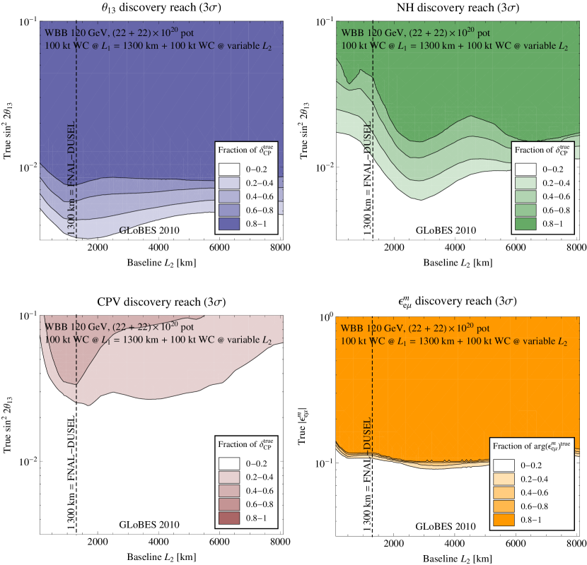
Figure 6: The dependence of various sensitivities, as labeled in the legend of each panel, on the baseline $L_{2}$ of a second detector. Shown are lines of constant CP fraction in the $L_{2}$–$\sin^{2}\theta_{13}^{\rm true}$ resp. $L_{2}$–$|(\varepsilon^{m}_{e\mu})^{\rm true}|$ plane. The results are given at $3\,\sigma$ confidence level.

An altogether different way to access events in the $2^{\mathrm{nd}}$ oscillation maximum is to use a second detector at a longer baseline. If the two detectors are to be in the same beam and the first one is on-axis, the second one has to be off-axis due to the curvature of the Earth’s surface. Alternatively, one can also imagine scenarios in which both detectors are off-axis, either with identical off-axis angles or with different ones. For example, in the T2KK setup Ishitsuka et al. (2005); Dufour et al. (2010), it has been proposed to use Super-Kamiokande (or a larger Water Čerenkov detector at the same site) as the detector sensitive to the $1^{\mathrm{st}}$ maximum, and supplement it with a second Water Čerenkov detector at a baseline of about $1,000\,\mathrm{km}$ on the east coast of Korea. Another proposal Badertscher et al. (2008) puts a liquid Argon detector at about $600\,\mathrm{km}$ on the island of Okinoshima. In both cases, due to the different off-axis angles, the second detector will be predominantly sensitive to the $2^{\mathrm{nd}}$ maximum. A superficial comparison of the obtainable sensitivities indicates a similar physics performance, where most of the differences is attributable to the different overall exposure Barger et al. (2007). In order to allow for a direct comparison with the results derived in this paper, we refrain from comparing these setups in detail and study instead the effects of the addition of a second baseline to the setup we have introduced in section III.1. Since we are interested in the question of the general impact the $2^{\mathrm{nd}}$ maximum can have, we will neglect the actual geometry and assume that we have two identical beams, which allows us to put the second detector on-axis into this second beam. This is clearly an unrealistic and overly optimistic assumption. It amounts to doubling the number of protons on target and in contrast to the proposals centered around Super-Kamiokande, which all exploit a single beam, leads to higher event rates in the $2^{\mathrm{nd}}$ maximum due to it being accessed in an on-axis beam. However, it allows us to estimate the maximum effect that events from the $2^{\mathrm{nd}}$ maximum could have under ideal circumstances. In other words, if we do not observe an overwhelming increase in performance under these most favorable conditions, then we can safely conclude that the $2^{\mathrm{nd}}$ oscillation maximum, despite its theoretical merits, in practice is not useful in a superbeam experiment. The results of this analysis are shown in figure 6. For the measurement of $\theta_{13}$ and CP violation, the performance optimum occurs for a detector location very close to $1,300\,\mathrm{km}$, which is the position of the first detector. The sensitivity to the mass hierarchy shows a strong preference of baselines around $2,500\,\mathrm{km}$, but we remark that a similar effect is also seen with only one detector, see figure 10 and also reference Barger et al. (2006). Interestingly, at this distance the first oscillation minimum is at the peak of the beam flux and thus both the $1^{\mathrm{st}}$ and $2^{\mathrm{nd}}$ maximum contribute about equally to the rate.

A further question is whether information from the $2^{\mathrm{nd}}$ maximum can help in determining the octant of $\theta_{23}$. To this end we computed the sensitivity to the octant in the same way as shown in figure 4 but constraining the data to the $1^{\mathrm{st}}$ maximum only. The results are identical to the one in figure 4; thus, we find that data from the $2^{\mathrm{nd}}$ maximum does not improve the senstivity to discern the octant of $\theta_{23}$.

The conclusion for three flavor oscillation in this case is the same as with only one detector: The $2^{\mathrm{nd}}$ maximum does not help with the measurement of $\theta_{13}$ or the CP phase, but it enhances the ability to measure the mass hierarchy. The gains in mass hierarchy sensitivity could be substantial under favorable conditions, but are only moderate in practice.

IV.3 Non-standard Interactions

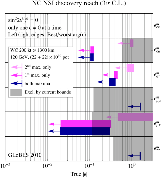
Figure 7: Discovery reach for neutral-current-like NSI in a WC detector (colored bars and arrows), compared to current model-independent limits on the different parameters Davidson et al. (2003); Gonzalez-Garcia and Maltoni (2008); Biggio et al. (2009) (gray shaded regions). The length of the colored bars is due to the unknown phase associated with the new interaction.

Next we turn our attention to the question whether the $2^{\mathrm{nd}}$ maximum is useful for new physics searches. For a given set of oscillation parameters the relative strength of the signals in the $1^{\mathrm{st}}$ and $2^{\mathrm{nd}}$ maximum is well understood within the standard three flavor oscillation framework, and therefore any deviation should stem from new physics. In order to be able to perform a quantitative analysis of this problem, we will restrict the new physics to the form of non-standard interactions, their underlying physics and parametrization have been described in section II.2.

In figure 7 the discovery reach for neutral current like NSI is shown for our standard setup. For each set of bars, only one NSI parameter was allowed to be nonzero at a time, i.e. we do not include correlations between different NSI parameters. The length of the bars is due to the unknown phase of the non-standard parameters, whereas the different colors are for different subsets of the data as explained in the legend. The gray shaded areas indicate the current model independent bounds on these parameters Davidson et al. (2003); Gonzalez-Garcia and Maltoni (2008); Biggio et al. (2009); in cases where there is no gray shaded area, the current bounds are of order one. Note that possible correlations between $\varepsilon^{m}_{ee}$ and other parameters are equivalent to correlations with the matter density, which are included in our simulations by the matter density uncertainty. Also, correlations between $\varepsilon^{m}_{e\mu}$, $\varepsilon^{m}_{e\tau}$ and the $\mu$–$\tau$ sector ($\varepsilon^{m}_{\mu\mu}$, $\varepsilon^{m}_{\mu\tau}$, $\varepsilon^{m}_{\tau\tau}$) are small because $\varepsilon^{m}_{e\mu}$ and $\varepsilon^{m}_{e\tau}$ affect mainly the appearance channel, while $\varepsilon^{m}_{\mu\mu}$, $\varepsilon^{m}_{\mu\tau}$ and $\varepsilon^{m}_{\tau\tau}$ are most relevant in the disappearance channel, see e.g. references Kopp et al. (2008); Kopp (2009); this has been shown for the $\varepsilon^{m}_{e\tau}$–$\varepsilon^{m}_{\tau\tau}$ correlation by explicit numerical calculation in Ref. Kopp et al. (2008). The strongest improvement in bounds happens for flavor-changing NSI, but this improvement is hardly dependent on the data from the $2^{\mathrm{nd}}$ oscillation maximum. The results for a liquid argon detector are very similar and lead to the same conclusion.

Based on our somewhat negative result with respect to the $2^{\mathrm{nd}}$ maximum in the case of standard three-flavor oscillation, we can study the effect of an artificial enhancement of statistics in the $2^{\mathrm{nd}}$ maximum also in the presence of non-standard interactions. The result of rescaling the flux according to equation 10 is shown in the lower right hand panel of figure 5 for the case of NSI in the $e$–$\mu$ sector. The performance optimum occurs at $x_{2}<1$, which implies that the $2^{\mathrm{nd}}$ maximum is not useful in this case. The option of using a second detector to access the $2^{\mathrm{nd}}$ maximum exists also for NSI studies and the result is shown in the lower right hand panel of figure 6. With a second detector between $3,000-6,000\,\mathrm{km}$ the sensitivity would be improved by less than a factor of two. The wide baseline range over which this improvement happens makes it seem unlikely that this is entirely due to the $2^{\mathrm{nd}}$ maximum. Also, in contrast to the case of the mass hierarchy measurement, where there was an improvement both for rescaling the flux and considering a second detector, here we see improvement only for the second detector, which points to overall increased matter effects, standard and non-standard, as the source of this improvement. Qualitatively a similar improvement is obtained by just using one detector at a longer baseline as shown in figure 10. In any case, the improvement is relatively moderate.

The previous statement about the relative unimportance of correlations between NSI parameters does not hold if one allows for the simultaneous presence of non-standard effects in the neutrino production, propagation, and detection processes. In particular, in this case the so called confusion theorem obtains Huber et al. (2002): Assume that $\theta_{13}=0$, but there are charged current NSI between $\nu_{\tau}$ and electrons in the detector ($\epsilon_{\tau e}^{d}\neq 0$), and neutral current NSI between $\nu_{e}$ and $\nu_{\tau}$ in the propagation ($\epsilon_{e\tau}^{m}\neq 0$). If we furthermore assume that the parameters obey the relation

$$\epsilon_{\tau e}^{d}=r\epsilon_{e\tau}^{m}\,,$$ (11)

with $r$ being an order one parameter determined by whether the NSI couple to quarks or leptons, then the event rate spectra for both neutrinos and anti-neutrinos in the $\nu_{\mu}\rightarrow\nu_{e}$ channel are the same as for standard three-flavor oscillations with

$$\sin^{2}\theta_{13}=r^{2}(\epsilon_{e\tau}^{m})^{2}\frac{1+\cos 2\theta_{23}}{2}\,.$$ (12)

This is the confusion theorem. Subsequently, it was discovered that for sufficiently high beam energies, muons from the decay of $\tau$ from $\nu_{\tau}$ charged current interactions can be used to resolve the confusion at least for parts of the parameters space Campanelli and Romanino (2002). For the setup considered here, the average beam energy is close to $m_{\tau}$, and therefore $\tau$-production in charged current interactions from $\nu_{\tau}$ will be strongly suppressed, and therefore no muons from $\tau$-decays will be observed. Thus, the confusion theorem should apply. Still, it is important to note that equations 11 and 12 were obtained from a perturbative expansion of the oscillation probability. This expansion is strictly valid only for energies around the $1^{\mathrm{st}}$ maximum. Thus the question arises to which degree the confusion theorem applies to the wide band scenario considered here.

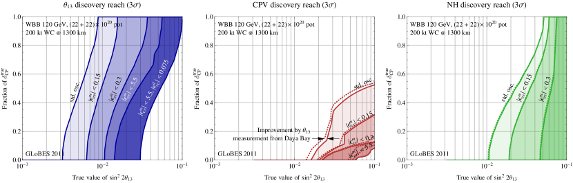
Figure 8: Discovery reach for $\sin^{2}2\theta_{13}$, $\delta_{\mathrm{CP}}$ and the mass hierarchy in the presence of NSI in propagation and detection, specifically $\varepsilon^{m}_{e\tau}$ and $\varepsilon^{d}_{\tau e}$. In all panels, the leftmost line is the usual three flavor oscillation result and the other lines are obtained by successively allowing NSI up to the limit indicated by the labels next to each line. The rightmost curves, corresponding to the current $3\,\sigma$ limits on the NSI parameters Davidson et al. (2003); Biggio et al. (2009), lie outside the plot for $\delta_{\mathrm{CP}}$ and the mass hierarchy. The dashed lines in the middle and right panels are the corresponding results if one assumes $\theta_{13}$ to be constrained by a measurement at Daya Bay.

A partial answer is shown in figure 8, where the sensitivity to $\sin^{2}2\theta_{13}$, CP violation and the mass hierarchy is depicted for various levels of NSI. The different lines are obtained by allowing successively larger values of $|\epsilon^{m}_{e\tau}|$ and $|\epsilon^{d}_{\tau e}|$ in the fit, as indicated in the plots. The largest values used in figure 8 correspond to the current $3\,\sigma$ bounds according to references Davidson et al. (2003); Biggio et al. (2009). In the left panel ($\theta_{13}$ discovery reach) and in the right panel (discovery reach for the normal mass hierarchy), we allow $\epsilon^{m}_{e\tau}$ and $\epsilon^{d}_{\tau e}$ to be complex with arbitrary phases, while in the middle panel (discovery reach for CP violation), we assume the phases of the NSI parameters to be $0$ or $\pi$ since we want to consider only CP conserving solutions in the fit. The rightmost line in the left hand panel of figure 8 confirms the validity of the confusion theorem in equations 11 and 12: We indeed observe a deterioration of the sensitivity by nearly an order of magnitude in $\sin^{2}2\theta_{13}^{\rm true}$. However, at the same time we see that $\epsilon^{m}_{e\tau}$ alone accounts for most of this deterioration since the difference between the rightmost line and the line next to it is relatively small. Thus, the confusion theorem seems to apply in essence, but in practice the small number of events around the sensitivity limit does not require the presence of NSI both in propagation and detection, because spectral information is not statistically significant. For the same reason, the information from the $2^{\mathrm{nd}}$ maximum plays no role, since at the sensitivity limit the event sample from the $2^{\mathrm{nd}}$ maximum is statistically not significant. We have performed the same scaling analysis as presented in figure 5 also in this case and find that the $2^{\mathrm{nd}}$ maximum is not useful in controlling the effects of NSI in propagation and detection.

In the middle panel of figure 8 we show the impact of NSI on the ability to discover CP violation, and the result exhibits the same qualitative features as the one for the discovery of $\theta_{13}$. At a quantitative level, this measurement is more sensitive to the deleterious effects of NSI since it relies on smaller, more difficult signatures also in the standard oscillation case. Therefore, we observe a complete loss of discovery potential for values of the NSI an order of magnitude below the current bounds. One may speculate that using a precision measurement of $\theta_{13}$ by the Daya Bay experiment could mitigate the correlation with NSI, however, as the dashed lines conclusively demonstrate, this is note the case. Thus, at the current level of analysis we are forced to conclude that the ability to discover leptonic CP violation in the next generation of superbeam experiments is not robust with respect to the presence of new physics. Neither a $\theta_{13}$ measurement by Daya Bay nor events from the $2^{\mathrm{nd}}$ maximum can resolve this problem. A direct measurement of $\epsilon^{m}_{e\tau}$ in a short-baseline neutral current neutrino scattering experiment to improve the upper limits is out of question, since this would require to measure the flavor of the outgoing neutrino. As shown in figure 4 of reference Huber et al. (2002), combining different baselines does not affect the validity of the confusion theorem and therefore does not present a viable strategy to address the confusion problem either.

In the rightmost panel of figure 8 we show how much the discovery reach for the mass hierarchy is diminished, and the result is equally drastic as in the case of CP violation.

A near detector can help to improve bounds on NSI in the neutrino production and detection processes, but our results show that NSI in propagation alone are sufficient to cause serious problems for the measurement of the standard oscillation parameters. Besides, a direct measurement of $\epsilon^{d}_{\tau e}$ is a difficult proposition for a number of reasons. First, there are no $\nu_{\tau}$ in the beam, so the only way of constraining $\epsilon^{d}_{\tau e}$ would be to constrain $\epsilon^{s}_{e\tau}$ instead and to make use of the fact that the two parameters are usually related since they can both arise from the same non-standard coupling between two light quarks, an electron, and a $\nu_{\tau}$ Kopp et al. (2008). However, this relation between $\epsilon^{d}_{\tau e}$ and $\epsilon^{s}_{e\tau}$ is not model-independent. For instance, a parity-conserving non-standard operator can lead to nonzero $\epsilon^{d}_{\tau e}$, but will not contribute to neutrino production in pion decay, so that $\epsilon^{s}_{e\tau}=0$ Kopp et al. (2010). Moreover, even measuring $\epsilon^{s}_{e\tau}$ is very challenging because the initial flux of electron neutrinos in an LBNE-like beam is very small, less than 1%, the kinematic suppression of $\tau$-production is large with the available beam energy, and $\tau$-identification is notoriously difficult and typically has a low efficiency. For these reasons, we conclude that near detectors will not solve the problem of possible confusion between standard oscillations and NSI. The specific setup considered here is in some sense a best case scenario, since it has relatively high statistics, a lot of spectral information, and makes use of two oscillation maxima. There is no reason to expect that experiments like T2K and NO$\nu$A will be less affected by the confusion problem, quite the contrary, as shown in reference Kopp et al. (2008).

V Summary and conclusions

The goal of this paper is to quantitatively understand the benefits, or lack thereof, of studying two oscillation maxima simultaneously in a long-baseline neutrino oscillation experiment. To this end we have chosen a specific example of experimental setup, which closely resembles the current plans for the Fermilab–DUSEL Long Baseline Neutrino Experiment (LBNE). There are two ways to access the $2^{\mathrm{nd}}$ oscillation maximum: either using a broad neutrino energy spectrum to cover the $1^{\mathrm{st}}$ and $2^{\mathrm{nd}}$ maximum in the same detector, or using two detectors at different baselines in the same beam. In LBNE, the natural method is to use the same detector and a wide energy spectrum. For this approach we found that there is no apparent benefit from using the $2^{\mathrm{nd}}$ maximum (figure 5). This remains true even if it were possible to shift a larger portion of the total neutrino flux into the energy range of the $2^{\mathrm{nd}}$ oscillation maximum. The measurement of the mass hierarchy does improve with events from the $2^{\mathrm{nd}}$ maximum, but the improvement is limited, and since it would come at the cost of losing events in the $1^{\mathrm{st}}$ maximum, which in turn negatively impacts the other measurements, a trade-off between these conflicting requirements has to be found. We have also investigated the option of using the same beam but two detectors at different baselines, which is the natural option for extensions of T2K Ishitsuka et al. (2005); Dufour et al. (2010); Badertscher et al. (2008). The results are similar to the previous case for the measurement of $\theta_{13}$ and CP violation, while the improvement in the sensitivity to the mass hierarchy is somewhat stronger in this case due to larger matter effects at the longer baseline (figure 6). As far as the possible detection of new physics—parametrized here in the framework of neutral current non-standard interactions (NSI)—is concerned, the sensitivity improves slightly for a second detector at a longer baseline. Note that neutral current NSI measurements prefer longer baselines in general since they essentially correspond to new neutrino matter effects, and matter effects are larger at long baseline. Therefore a similar improvement can also be observed for a single detector setup with a longer baseline (figure 10).

Finally, we have revisited the so called confusion theorem, which has been discovered in the context of neutrino factories Huber et al. (2002). The confusion theorem states that certain combinations of charged and neutral current NSI modify the neutrino oscillation probability in the same way as a nonzero value of $\theta_{13}$ does. In particular, the effects of the NSI parameter $\epsilon^{m}_{e\tau}$ are problematic since this parameter is only weakly constrained by an $\mathcal{O}(1)$ bound. In other words, in the absence of sufficiently strong bounds on NSI, it is very hard to establish a bound on $\theta_{13}$. In the context of neutrino factories, muons from $\tau$ decays have proven to be a loophole in the confusion theorem Campanelli and Romanino (2002), but in a superbeam experiment the beam energy is so low that $\tau$-production is kinematically suppressed and the arguments from reference Campanelli and Romanino (2002) do not apply, as has been shown in the context of T2K and NO$\nu$A Kopp et al. (2008). In the present work we have extended those earlier results to superbeam experiments which have events from the $1^{\mathrm{st}}$ and $2^{\mathrm{nd}}$ oscillation maximum. We have found that the confusion theorem holds (figure 8) and the sensitivity to $\sin^{2}2\theta_{13}$ deteriorates by one order of magnitude if the possibility of NSI is taken into account. Data from the $2^{\mathrm{nd}}$ maximum has no effect on this conclusion since it is statistically not significant enough. Moreover, we have shown that even the effect of neutral current NSI ($\epsilon_{e\tau}^{m}\neq 0$) alone is sufficient to seriously impact the sensitivity to $\sin^{2}2\theta_{13}$. This is an especially problematic limitation since $\epsilon_{e\tau}^{m}$ cannot be constrained by a near detector measurement. For CP violation measurements, the possibility of complex $\epsilon_{e\tau}^{m}$ has been considered and the impact is dramatic: Even for $\epsilon_{e\tau}^{m}$ an order of magnitude below the current bound a complete loss of sensitivity ensues. Reactor experiments will not be affected by $\epsilon_{e\tau}^{m}$ and thus can provide a clean measurement of $\sin^{2}2\theta_{13}$, but we have shown that even precise knowledge of $\theta_{13}$ from a reactor experiment does not solve the problem. The presence of data from the $2^{\mathrm{nd}}$ maximum does not provide immunity from the confusion theorem and it has an overall very small quantitative impact. This remains true even if the majority of the neutrino flux were shifted into the $2^{\mathrm{nd}}$ maximum. In comparison, T2K and NO$\nu$A have smaller statistics and observe a much smaller range in $L/E$. Therefore, the impact of the confusion theorem is more severe in these experiments Kopp et al. (2008).

To put our conclusion on the possible impact of large NSI into perspective, we should emphasize that NSI large enough to be problematic for T2K, NO$\nu$A, or LBNE, are not a generic prediction of extensions of the Standard Model. In particular, from a model-builder’s point of view, new particles at or above the electroweak scale are rather unlikely to have a sizable effect on the neutrino sector Antusch et al. (2009); Gavela et al. (2009). On the other hand, new physics at a low scale may still lead to large NSI Joshipura and Mohanty (2004); Nelson and Walsh (2008), and since neutrino physics has taught us in the past that theorists’ prejudices may be wrong, one cannot discard such possibilities.

In summary, we find that only the determination of the mass hierarchy benefits slightly from using the $2^{\mathrm{nd}}$ oscillation maximum in a long baseline neutrino oscillation experiment. All other measurements, including non-standard neutrino interactions, are not improved compared to the case where only events from the $1^{\mathrm{st}}$ maximum are used. We confirm that the “confusion theorem”, which states that certain types of NSI can mimic the effects of nonzero $\theta_{13}$, remains valid even if data from the $2^{\mathrm{nd}}$ maximum is available. In particular, we have shown that the presence of a non-standard coupling between electron neutrinos and $\tau$ neutrinos with a complex coefficient $\epsilon_{e\tau}^{m}$ can completely destroy the sensitivity to CP violation and the mass hierarchy. Since it is known from the literature Huber et al. (2002) that combining different baselines does not alleviate this problem, and we have explicitly shown that adding reactor neutrino data does not work to this end either, it seems that there are no simple remedies for the confusion problem.

Acknowledgments

We are indebted to the members of the LBNE collaboration, especially Mary Bishai, Bonnie Fleming, Roxanne Guenette, Gina Rameika, Lisa Whitehead, and Geralyn ‘Sam’ Zeller for providing invaluable information on the parameters of the planned Fermilab neutrino beams, DUSEL detectors, and other aspects of the LBNE experiment. We are also grateful to Mattias Blennow for some very useful discussions, especially during the early stages of this project. PH would like to acknowledge the warm hospitality at the Astroparticle Physics - A Pathfinder to New Physics workshop at the KTH in Stockholm, during which this project was conceived, and the $\nu$TheME institute at CERN, where it was brought to completion.

Fermilab is operated by Fermi Research Alliance, LLC under Contract No. DE-AC02-07CH11359 with the US Department of Energy. This work has been in part supported by the US Department of Energy under award number DE-SC0003915.

Appendix A Possible alternative setups

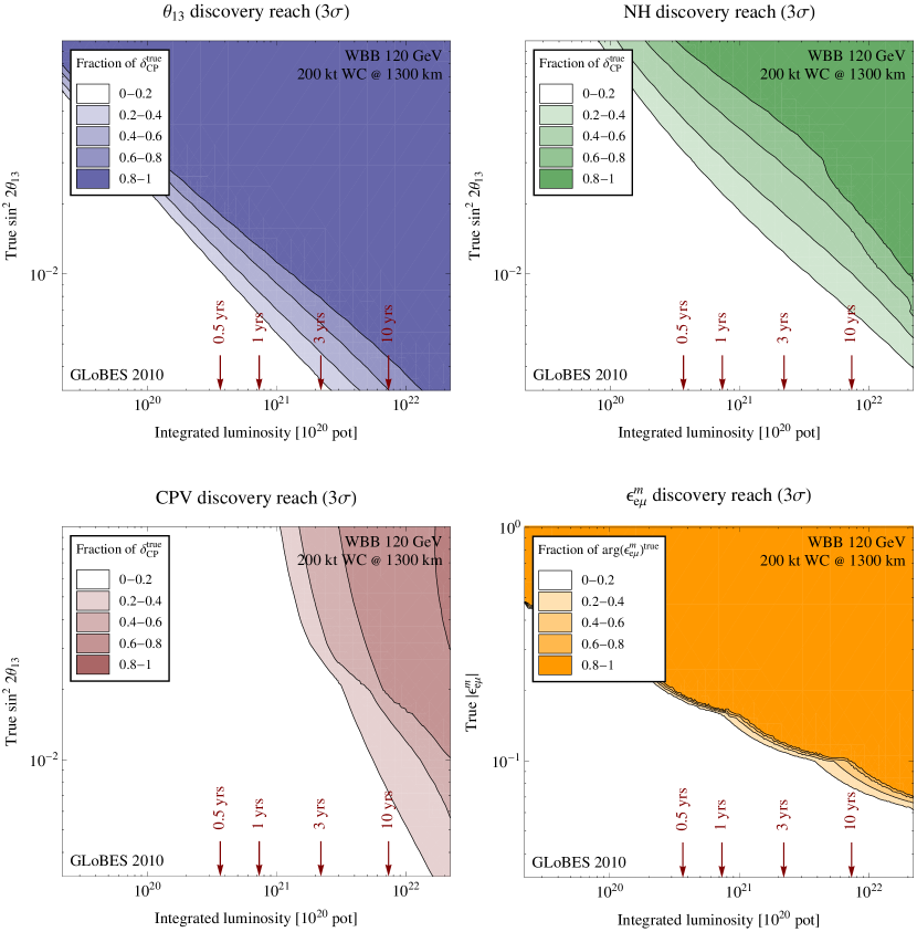
Figure 9: WBB discovery reach as a function of the exposure. The vertical, red arrows indicate the running time required with the standard value of $7.3\times 10^{20}\,\mathrm{pot}\,\mathrm{y}^{-1}$ at $120\,\mathrm{GeV}$. All plots are for a $200\,\mathrm{kt}$ WC detector. The curves indicate different CP fractions as given in the legend.

In this appendix we study simple variations of the basic experimental setup considered in this paper. The results given here will allow to extrapolate the effects of changes in the exposure and baseline. In figure 9 we show the discovery reach for standard oscillation as well as NSI as a function of exposure. Obviously, the higher the exposure the better the sensitivity. Discovery of CP violation has the largest demand for high exposure and conversely is most at risk if the luminosity were to turn out smaller than expected.

Figure 10 illustrates the dependence of the discovery reaches for $\theta_{13}$, mass hierarchy, CPV discovery and the NSI parameter $\epsilon_{e\mu}^{m}$ as a function of the baseline. The lines and corresponding shades are iso-contours of CP fraction. The optimum occurs for CP violation and the discovery of $\theta_{13}$ around $1,500\,\mathrm{km}$, whereas the optimum for the discovery of the mass hierarchy and $\epsilon_{e\mu}^{m}$ is around $2,200\,\mathrm{km}$. This result confirms that $L=1,300\,\mathrm{km}$ is a reasonable comprise for the neutrino beam assumed in this paper, and slightly longer baselines around $1,600\,\mathrm{km}$ would perform very similarly.

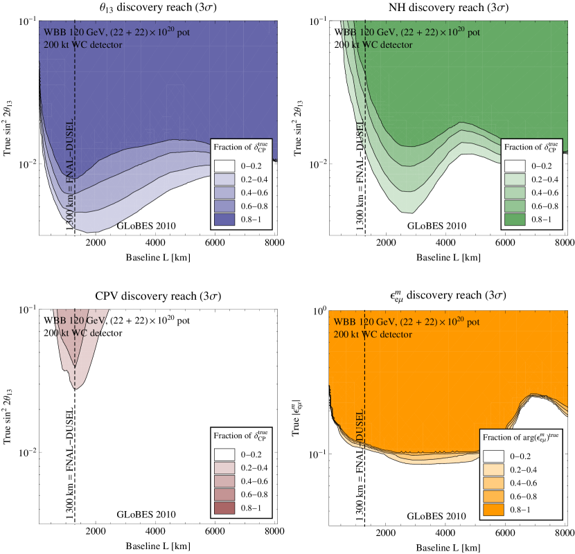
Figure 10: WBB discovery reach as a function of the baseline using a 200 kt WC detector. The lines and the corresponding shades are iso-contours of CP fraction with values given in the legend. The four panels are in the top row: $\theta_{13}$ discovery reach (left) and mass hierarchy discovery reach (right). In the lower row we have: discovery reach for CP violation (left) and discovery reach for the NSI parameter $\epsilon_{e\mu}^{m}$ as one example of NSI sensitivities. All results are shown at the $3\,\sigma$ confidence level.

References

- Aguilar et al. (2001) A. Aguilar et al. (LSND), Phys. Rev., D64, 112007 (2001), hep-ex/0104049 .
- Athanassopoulos et al. (1998) C. Athanassopoulos et al. (LSND), Phys. Rev., C58, 2489 (1998), arXiv:nucl-ex/9706006 .
- Athanassopoulos et al. (1995) C. Athanassopoulos et al. (LSND), Phys. Rev. Lett., 75, 2650 (1995), arXiv:nucl-ex/9504002 .
- Aguilar-Arevalo et al. (2007) A. A. Aguilar-Arevalo et al. (The MiniBooNE), Phys. Rev. Lett., 98, 231801 (2007), arXiv:0704.1500 [hep-ex] .
- Aguilar-Arevalo et al. (2009) A. A. Aguilar-Arevalo et al. (MiniBooNE), Phys. Rev. Lett., 102, 101802 (2009), arXiv:0812.2243 [hep-ex] .
- Aguilar-Arevalo et al. (2010) A. A. Aguilar-Arevalo et al. (The MiniBooNE), (2010), arXiv:1007.1150 [hep-ex] .
- Gonzalez-Garcia and Maltoni (2008) M. C. Gonzalez-Garcia and M. Maltoni, Phys. Rept., 460, 1 (2008), arXiv:0704.1800 [hep-ph] .
- Maltoni et al. (2004) M. Maltoni, T. Schwetz, M. A. Tortola, and J. W. F. Valle, New J. Phys., 6, 122 (2004), hep-ph/0405172 .
- Anderson et al. (2004) K. Anderson et al., (2004), hep-ex/0402041 .
- Ardellier et al. (2004) F. Ardellier et al., (2004), hep-ex/0405032 .
- Ahn et al. (2010) J. K. Ahn et al. (RENO), (2010), arXiv:1003.1391 [hep-ex] .
- Guo et al. (2007) X. Guo et al. (Daya-Bay), (2007), arXiv:hep-ex/0701029 .
- Huber et al. (2009) P. Huber, M. Lindner, T. Schwetz, and W. Winter, JHEP, 11, 044 (2009), arXiv:0907.1896 [hep-ph] .
- Mezzetto and Schwetz (2010) M. Mezzetto and T. Schwetz, (2010), arXiv:1003.5800 [hep-ph] .
- Itow et al. (2001) Y. Itow et al., Nucl. Phys. Proc. Suppl., 111, 146 (2001), hep-ex/0106019 .
- Ayres et al. (2004) D. S. Ayres et al. (NOvA), (2004), hep-ex/0503053 .
- Bandyopadhyay et al. (2007) A. Bandyopadhyay et al. (ISS Physics Working Group), (2007), arXiv:0710.4947 [hep-ph] .
- Akhmedov et al. (2004) E. K. Akhmedov, R. Johansson, M. Lindner, T. Ohlsson, and T. Schwetz, JHEP, 04, 078 (2004), hep-ph/0402175 .
- Burguet-Castell et al. (2001) J. Burguet-Castell, M. B. Gavela, J. J. Gomez-Cadenas, P. Hernandez, and O. Mena, Nucl. Phys., B608, 301 (2001), arXiv:hep-ph/0103258 .
- Minakata and Nunokawa (2001) H. Minakata and H. Nunokawa, JHEP, 10, 001 (2001), hep-ph/0108085 .
- Fogli et al. (1997) G. L. Fogli, E. Lisi, D. Montanino, and G. Scioscia, Phys. Rev., D55, 4385 (1997), arXiv:hep-ph/9607251 .
- Barger et al. (2002) V. Barger, D. Marfatia, and K. Whisnant, Phys. Rev., D65, 073023 (2002), hep-ph/0112119 .
- Minakata and Uchinami (2010) H. Minakata and S. Uchinami, JHEP, 04, 111 (2010), arXiv:1001.4219 [hep-ph] .
- Huber et al. (2002) P. Huber, M. Lindner, and W. Winter, Nucl. Phys., B645, 3 (2002a), hep-ph/0204352 .
- Winter (2004) W. Winter, Phys. Rev., D70, 033006 (2004), arXiv:hep-ph/0310307 .
- Joshipura and Mohanty (2004) A. S. Joshipura and S. Mohanty, Phys. Lett., B584, 103 (2004), arXiv:hep-ph/0310210 .
- Nelson and Walsh (2008) A. E. Nelson and J. Walsh, Phys.Rev., D77, 033001 (2008), arXiv:arXiv:0711.1363 [hep-ph] .
- Gavela et al. (2009) M. B. Gavela, D. Hernandez, T. Ota, and W. Winter, Phys. Rev., D79, 013007 (2009), arXiv:0809.3451 [hep-ph] .
- Antusch et al. (2009) S. Antusch, J. P. Baumann, and E. Fernandez-Martinez, Nucl. Phys., B810, 369 (2009), arXiv:0807.1003 [hep-ph] .
- Kopp et al. (2008) J. Kopp, M. Lindner, T. Ota, and J. Sato, Phys. Rev., D77, 013007 (2008a), arXiv:0708.0152 [hep-ph] .
- Kopp (2009) J. Kopp, “New phenomena in neutrino physics,” (2009), Ph.D. thesis, University of Heidelberg, available from http://www.ub.uni-heidelberg.de/archiv/9381.
- Davidson et al. (2003) S. Davidson, C. Pena-Garay, N. Rius, and A. Santamaria, JHEP, 03, 011 (2003), hep-ph/0302093 .
- Biggio et al. (2009) C. Biggio, M. Blennow, and E. Fernandez-Martinez, (2009), arXiv:0907.0097 [hep-ph] .
- Blennow et al. (2008) M. Blennow, D. Meloni, T. Ohlsson, F. Terranova, and M. Westerberg, Eur. Phys. J., C56, 529 (2008), arXiv:0804.2744 [hep-ph] .
- Friedland and Lunardini (2005) A. Friedland and C. Lunardini, Phys. Rev., D72, 053009 (2005), hep-ph/0506143 .
- Huber et al. (2005) P. Huber, M. Lindner, and W. Winter, Comput. Phys. Commun., 167, 195 (2005), http://www.mpi-hd.mpg.de/lin/globes/, hep-ph/0407333 .
- Huber et al. (2007) P. Huber, J. Kopp, M. Lindner, M. Rolinec, and W. Winter, Comput. Phys. Commun., 177, 432 (2007), hep-ph/0701187 .
- Kopp et al. (2007) J. Kopp, M. Lindner, and T. Ota, Phys. Rev., D76, 013001 (2007), hep-ph/0702269 .
- Kopp (2008) J. Kopp, Int. J. Mod. Phys., C19, 523 (2008), erratum ibid. C19 (2008) 845, arXiv:physics/0610206 .
- Bishai (2010) M. Bishai, (2010), private communication.
- Yanagisawa et al. (2007) C. Yanagisawa, C. K. Jung, P. T. Le, and B. Viren, AIP Conf. Proc., 944, 92 (2007).
- Dufour et al. (2010) F. Dufour, T. Kajita, E. Kearns, and K. Okumura, Phys. Rev., D81, 093001 (2010), arXiv:1001.5165 [hep-ph] .
- Barger et al. (2006) V. Barger et al., Phys. Rev., D74, 073004 (2006), arXiv:hep-ph/0607177 .
- Diwan et al. (2006) M. Diwan et al., (2006), arXiv:hep-ex/0608023 .
- Fleming and Zeller (2008) B. Fleming and G. Zeller, (2008), private communication.
- Barger et al. (2007) V. Barger, P. Huber, D. Marfatia, and W. Winter, Phys. Rev., D76, 031301 (2007), arXiv:hep-ph/0610301 .
- Messier (1999) M. D. Messier, Evidence for neutrino mass from observations of atmospheric neutrinos with Super-Kamiokande, Ph.D. thesis, Boston University (1999), UMI-99-23965.
- Paschos and Yu (2002) E. A. Paschos and J. Y. Yu, Phys. Rev., D65, 033002 (2002), hep-ph/0107261 .
- Ishitsuka et al. (2005) M. Ishitsuka, T. Kajita, H. Minakata, and H. Nunokawa, Phys. Rev., D72, 033003 (2005), arXiv:hep-ph/0504026 .
- Badertscher et al. (2008) A. Badertscher et al., (2008), arXiv:0804.2111 [hep-ph] .
- Kopp et al. (2008) J. Kopp, T. Ota, and W. Winter, Phys. Rev., D78, 053007 (2008b), arXiv:0804.2261 [hep-ph] .
- Huber et al. (2002) P. Huber, T. Schwetz, and J. W. F. Valle, Phys. Rev., D66, 013006 (2002b), arXiv:hep-ph/0202048 .
- Campanelli and Romanino (2002) M. Campanelli and A. Romanino, Phys. Rev., D66, 113001 (2002), hep-ph/0207350 .
- Kopp et al. (2010) J. Kopp, P. A. N. Machado, and S. J. Parke, (2010), arXiv:1009.0014 [hep-ph] .