A Population of Very-Hot Super-Earths in Multiple-Planet Systems Should be Uncovered by Kepler

Abstract

We simulate a Kepler-like observation of a theoretical exoplanet population and we show that the observed orbital period distribution of the Kepler giant planet candidates is best matched by an average stellar specific dissipation function $Q_{\ast}^{\prime}$ in the interval $10^{6}\lesssim Q_{\ast}^{\prime}\lesssim 10^{7}$. In that situation, the few super-Earths that are driven to orbital periods $P<1$ day by dynamical interactions in multiple-planet systems will survive tidal disruption for a significant fraction of the main-sequence lifetimes of their stellar hosts. Consequently, though these very-hot super-Earths are not characteristic of the overall super-Earth population, their substantial transit probability implies that they should be significant contributors to the full super-Earth population uncovered by Kepler. As a result, the CoRoT-7 system may be the first representative of a population of very-hot super-Earths that we suggest should be found in multiple-planet systems preferentially orbiting the least-dissipative stellar hosts in the Kepler sample.

1. Introduction

NASA’s Kepler mission (Koch et al., 2010; Jenkins et al., 2010a; Caldwell et al., 2010; Bryson et al., 2010; Batalha et al., 2010a, b; Haas et al., 2010; Jenkins et al., 2010b) is currently searching for transiting planets in photometric observations of $\sim 156,000$ solar-type stars in a 115 deg² field of view in the constellation Cygnus toward the Orion arm of our Galaxy. Kepler photometric observations will achieve 80 parts per million precision over 80%-90% of the telescope field of view, sufficient to identify the transit signal from an Earth-Sun equivalent system. By the end of its four-year mission, the combination of Kepler’s unprecedented precision, sample size, and homogeneous selection will produce a near ideal set of exoplanet detections to compare with theoretical models of planet formation. Though the preliminary exoplanet candidate list announced in Borucki et al. (2010) is incomplete, it is still a valuable constrain on theoretical models of close-in planet formation.

In the core accretion model of close-in planet formation (e.g., Pollack et al., 1996; Ida & Lin, 2004), the cores of giant planets form near the ice line of their parent protoplanetary disk. The cores grow to an isolation mass and accrete gas until they are massive enough to open-up a gap in their parent disk. The newly-formed giant planets then Type II migrate into the close proximity of their host star and stop inside the magnetospheric truncation radius of their parent protoplanetary disk (e.g., Lin et al., 1996). Lower-mass planets in the close proximity of their host stars result from the inward Type I migration (Ward, 1997) of planetary embryos that did not reach the mass necessary to initiate runaway accretion of gas and become giant planets. These lower-mass close-in planets may be hot Neptunes or icy super-Earths that formed near the ice line of their parent protoplanetary disks and then migrated to just outside the disk magnetospheric truncation radius (e.g., Masset et al., 2006). Alternatively, they may be rocky Earth and super-Earth mass planets that formed interior to the ice line and then migrated either singly or in resonant planet convoys into the close proximity of their host star, eventually stopping just outside the disk magnetospheric truncation radius (e.g., Ida & Lin, 2010; Ogihara et al., 2010). Theoretical exoplanet population synthesis (EPS) models (Ida & Lin, 2008, 2010; Mordasini et al., 2009a, b) in the core accretion and migration paradigm have reproduced many trends in the observed distribution of exoplanet properties, and comparisons between observations and models are especially useful to constrain uncertain model parameters (e.g., Schlaufman et al., 2009).

Tidal interactions between close-in planets and their stellar hosts contribute significantly to the dynamical evolution of close-in planet systems after the dissipation of their parent protoplanetary disks (e.g., Rasio et al., 1996; Dobbs-Dixon et al., 2004). Tidal effects tend to circularize and shrink orbits to the point that close-in planets suffer substantial mass loss and eventually tidal disruption (e.g., Gu et al., 2003; Jackson et al., 2008a, 2009; Li et al., 2010). The efficiency and timescale for these processes are both uncertain (e.g., Levrard et al., 2009) and highly dependent on the internal structure of the close-in planet (e.g., Ogilvie & Lin, 2004) and its stellar host (e.g., Ogilvie & Lin, 2007; Barker & Ogilvie, 2009, 2010). Modeling of the properties of the close-in planet candidates identified by Kepler will help resolve some of these uncertainties.

In this letter, we combine an extended version of the EPS models of Ida & Lin (2010)–IL10 hereafter–with the mass–radius relations of Fortney et al. (2007) to extract the expected period–radius distribution of the extended EPS. We use Monte Carlo simulations in concert with a detailed model of Kepler sensitivity and a simple model of tidal evolution to determine the exoplanet period–radius distribution that Kepler would observe in the extended EPS as a function of the strength of tidal evolution. We then compare the result with the observed period distribution of Kepler transiting giant planet candidates announced in Borucki et al. (2010) to constrain the strength of tidal evolution in the Kepler candidate planet sample. We describe our Monte Carlo simulations and Kepler-like observations of the extended IL10 EPS in Section 2. We discuss the results and implications of our simulations in Section 3, and we summarize our findings in Section 4.

2. Analysis

Transit observations directly measure exoplanet radii and orbital periods, while radial velocity observations are necessary to confirm individual transit detections and to determine exoplanet masses. Unfortunately, most exoplanet candidates identified by Kepler will orbit host stars with faint apparent magnitudes. As a result, radial velocity follow-up will be telescope-time intensive for the more massive Kepler exoplanet candidates and possibly too imprecise at faint magnitudes to confirm lower-mass candidates. Consequently, it becomes important to carefully consider what insight can be gained from the exoplanet period distribution derived purely from Kepler transit photometry.

To that end, we use a Monte Carlo simulation to systematically observe an extended version of the IL10 EPS to as much as possible match Kepler observations of the Milky Way’s exoplanet population. In this case, we have extended the IL10 EPS such that the distribution of host stellar mass in the 10³ systems in the EPS matches the distribution of host stellar mass expected in Kepler observations. That is, we match the distribution of host stellar mass in the extended IL10 EPS to the mass distribution expected in a Kepler-like observation of the Reid & Hawley (2005) solar neighborhood luminosity function, given Kepler’s sensitivity as a function of host spectral type and apparent magnitude.

The first step in our calculation is to approximate the radius of each planet in the extended IL10 EPS. The IL10 models include the asymptotic semimajor axis, rock mass, ice mass, and gas mass of every planet. From those quantities, we use the mass–radius relations given in Fortney et al. (2007) to assign radii to giant planets as a function of semimajor axis, solid mass, and gas mass and to terrestrial planets as a function of solid mass and composition.

We then do 100 iterations of a Monte Carlo simulation in which we assign each planetary system in the extended IL10 EPS a random host stellar mass, age, and apparent magnitude, as well as a random orbital inclination. We assign each eccentric planet a random argument of periastron. We first randomly assign spectral types and apparent magnitudes to the host stars of the extended exoplanet population. We use the solar neighborhood luminosity function given in Table 8.3 of Reid & Hawley (2005) to determine the number density of FGK stars as a function of spectral type and apparent magnitude; we use this information to determine the probability that a randomly selected star from the Kepler field is of a given spectral type and apparent magnitude. The spectral type of the assigned host star determines the host stellar mass and radius.

To account for the effect of tidal evolution on the observability of the extended IL10 exoplanet population, we exploit the fact that the two-Gyr moving-average smoothed star formation history in the Milky Way has been more or less constant over the last $\sim 10$ Gyr (e.g., Rocha-Pinto et al., 2000a, b). As a result, the unknown age of a randomly selected star from a magnitude-limited survey of Milky Way disk stars with main-sequence lifetime $\tau_{\ast}$ short relative to that $\sim 10$ Gyr interval should be distributed more or less uniformly between zero and its main-sequence lifetime. Magnitude-limited transit surveys like Kepler are biased toward stars with $M_{\ast}\gtrsim 1~{}M_{\odot}$, and those stars have main-sequence lifetimes $\tau_{\ast}\lesssim 10$ Gyr. Consequently, the unknown system age $\tau_{\mathrm{sys}}$ of a typical candidate exoplanet system identified by Kepler in transit with host stellar mass $M_{\ast}$ should be well-approximated as uniformly distributed in the interval $0\leq\tau_{\mathrm{sys}}\leq\tau_{\ast}(M_{\ast})$. For that reason, in the Monte Carlo we randomly sample the age of each exoplanet system from a uniform distribution between zero and the main-sequence lifetime of its stellar host. For Sun-like stars $L_{\ast}(M_{\ast})=L_{\odot}~{}(M_{\ast}/M_{\odot})^{3.5}$ (e.g., Popper, 1980), and the total amount of hydrogen available for fusion is proportional to $M_{\ast}$. The main-sequence lifetime is roughly then $\tau_{\ast}(M_{\ast})=\tau_{\odot}~{}M_{\ast}/L_{\ast}(M_{\ast})=10~{}(M_{\ast}/M_{\odot})^{-2.5}$ Gyr. We consider an exoplanet observable if its randomly determined age $\tau_{\mathrm{sys}}$ is less than the timescale for the tidal evolution of its orbit to move it within $1~{}R_{\ast}$ of its stellar host $\tau_{\mathrm{dis}}$ at which point we assume that the planet is tidally disrupted and no longer observable (e.g., Sandquist et al., 1998). In other words, a planet is only observable if $\tau_{\mathrm{sys}}<\tau_{\mathrm{dis}}$. We define the time to disruption as (e.g., Ibgui & Burrows, 2009)

$$\tau_{\mathrm{dis}} = \frac{4}{117}\frac{a_{0}^{13/2}}{G^{1/2}}\frac{M_{\ast}^{1/2}}{M_{p}}\frac{Q_{\ast}^{\prime}}{R_{\ast}^{5}}\left[1-(R_{\ast}/a_{0})^{13/2}\right]\mathrm{,}$$ (1)

where $a_{0}$ is the initial semimajor axis of the planet before tidal evolution, $Q_{\ast}^{\prime}$ is the specific dissipation function of the host star, $G$ is Newton’s gravitational constant, $M_{p}$ is the mass of the planet, and $R_{\ast}$ is the radius of the host star. The expression given in Ibgui & Burrows (2009) is strictly valid only for circular orbits, so we assume that the timescale for eccentricity damping is short relative to $\tau_{\mathrm{dis}}$.

As a result of the assumptions we make in our treatment of tidal evolution, we assume that the all planets from the extended IL10 population with orbital period $P<10$ days are on circular orbits. We use the eccentricity distribution generated from the EPS models for longer-period systems. We sample the orbital inclination and argument of periastron from the standard random distributions of those quantities. We adopt the analytic formulae given in Seager & Mallén-Ornelas (2003) and Ford et al. (2008) to determine the transit depth and transit duration of every planet found to transit. Finally, we use a detailed model of Kepler sensitivity (D. Koch et al., private communication) that gives the threshold detectable exoplanet radius as a function of host spectral type, host apparent magnitude, transit depth, transit duration, and number of transits over a given duration of observation to determine which of the simulated transiting exoplanets would be detectable in the first 43 days of Kepler data.

We save the results of this iteration, and repeat our Monte Carlo simulation 100 times to average over all of the given distributions to generate a prediction for the characteristics of the planetary systems Kepler would likely identify in an exoplanet population matching the extended IL10 EPS. We carry out this Monte Carlo simulation for four fiducial values of $Q_{\ast}^{\prime}$: 10⁵ (strong tidal evolution), 10⁶ (moderate tidal evolution), 10⁷ (weak tidal evolution), and $\infty$ (no tidal evolution). We present the results of our simulations for each assumed value of $Q_{\ast}^{\prime}$ in Figures 1 to 4.

3. Discussion

The exoplanet period–radius distribution that results from a Kepler-like observation of the extended IL10 EPS is a strong function of $Q_{\ast}^{\prime}$. In the most dissipative case $Q_{\ast}^{\prime}=10^{5}$, hot Jupiters are quickly disrupted and the period distribution of giant planets is flat with a peak at $P\approx 10$ days. At the same time, the handful of planets at very short period $P<1$ day produced by dynamical interactions between planets in multiple-planet systems after the dissipation of their parent protoplanetary disk are tidally disrupted and unobservable in a Kepler-like observation. In the less dissipative cases $Q_{\ast}^{\prime}=10^{6}$ and $Q_{\ast}^{\prime}=10^{7}$, hot Jupiters survive for a significant fraction of the main-sequence lifetime of their host star and the period distribution of giant planets peaks in the range $3<P<5$ days in agreement with the giant planet period distribution in Borucki et al. (2010). In those cases, the observed period distribution of super-Earths would have a long tail toward periods shorter than one day. In the case with no tidal dissipation $Q_{\ast}^{\prime}=\infty$, hot Jupiters survive for the entire main-sequence lifetime of their stellar hosts and the period distribution of giant planets is a monotonically decreasing function of period. As a result, a Kepler-like observation would be dominated by planets with periods less than one day. Unlike the IL10 models, our calculations suggest that in the case of weak or no tidal evolution super-Earths should be observed to have a shorter average period than giant planets.

In Figure 5 we compare the giant planet period distribution that results from our simulated Kepler-like observation of the extended IL10 EPS with the Kepler planet-candidate period distribution from Borucki et al. (2010). Massive close-in planets are most sensitive to tidal evolution, so we only compare the period distribution of giant planets from the extended IL10 EPS more massive than $50~{}M_{\oplus}$ with those Kepler planet candidates with radii greater than 0.5 Jupiter radii. The Kepler planet candidates from Borucki et al. (2010) are not necessarily representative of the properties of the still-embargoed full sample of Kepler planet candidates. At the same time, the announced candidates are very likely those candidates unsuitable for radial velocity follow-up. For the massive planet candidates at least, that only indicates they orbit apparently faint host stars. Properties like the average metallicity of a stellar population are not a strong function of Galactocentric radius, so there is no reason to believe that the subsample of planets that orbit apparently faint stars at distances $d\sim 500$ pc from the Sun is systematically different than the subsample of planets that orbit apparently bright stars at distances $d\sim 200$ pc from the Sun. For those reasons, we argue that a comparison of the period distribution of the announced Kepler exoplanet candidates with the period distribution expected from a Kepler-like observation of the extended IL10 EPS under different assumptions for the strength of tidal evolution is meaningful.

The period distribution of the Kepler planet candidates is inconsistent with both strong tidal evolution and no tidal evolution given the extended IL10 EPS. The observed distribution is consistent with the two intermediate values of $Q_{\ast}^{\prime}=10^{6}$ and $Q_{\ast}^{\prime}=10^{7}$, with a better match provided by $Q_{\ast}^{\prime}=10^{7}$. This measurement is also consistent with the typically quoted $Q_{\ast}^{\prime}=10^{6}$ from the literature (e.g., Ogilvie & Lin, 2007).

The average specific dissipation function $Q_{\ast}^{\prime}=10^{7}$ suggested by our analysis implies that though very-hot super-Earths are not common, their substantial transit probability ensures that they will be readily observable by Kepler. We expect that about 10% of detected planets with $P<10$ days and $M_{p}<10~{}M_{\oplus}$ should be very-hot super-Earths with $P<1$ day. Very-hot super-Earths are produced by dynamical interactions in multiple-planet systems, and we suggest that very-hot super-Earths systems identified in transit surveys should frequently have observable companions (e.g., Mardling & Lin, 2004). Indeed, the very-hot super-Earth CoRoT-7b (Léger et al., 2009) is in a confirmed multiple system (Queloz et al., 2009) with the recently suggested possibility of a third planet (Hatzes et al., 2010). Very-hot super-Earths should also preferentially be found around Sun-like stars with $M_{\ast}\gtrsim 1.25~{}M_{\odot}$, as these stars are likely less dissipative than stars with $M_{\ast}\approx 1~{}M_{\odot}$ (Barker & Ogilvie, 2009). At the same time, there are other explanations for the properties of the CoRoT-7 system that match the observations (e.g., Jackson et al., 2010).

There are many limitations to our approach. We use only a single value of $Q_{\ast}^{\prime}$ to model the strength of tidal evolution regardless of host star age or spectral type, when is there is evidence from both observation (e.g., Schlaufman, 2010; Winn et al., 2010) and theoretical models (e.g., Barker & Ogilvie, 2009, 2010) that $Q_{\ast}^{\prime}$ is a function of host star age and stellar structure, as well as exoplanet orbital period. This issue will be resolved in the future when the full list of Kepler planet candidates is announced, as the increased host star statistics will allow us to do similar calculations in bins of host star effective temperature and thereby constrain $Q_{\ast}^{\prime}$ as a function of $T_{\mathrm{eff}}$ and therefore stellar structure. We do not simultaneously evolve the orbit and radius of the exoplanet population (e.g., Jackson et al., 2008b; Ibgui & Burrows, 2009; Miller et al., 2009), and the migration stopping conditions discussed in Section 2.5 of IL10 are also uncertain.

In IL10, planets that were massive enough to open-up a gap in their parent protoplanetary disk were stopped just inside the disk magnetospheric truncation radius (taken to be at $P=2$ days), while planets that were not massive enough to open-up a gap were stopped just outside of the magnetospheric truncation radius (taken to be at $P=3$ days). Though these stopping conditions are dependent on the uncertain properties of the parent protoplanetary disk (e.g., Lin et al., 1996; Masset et al., 2006; Ogihara et al., 2010), they are self-consistent in that they describe where an exoplanet of a given mass will stop if the stellar magnetic field and disk mass-accretion rate have a given value.

4. Conclusion

We coupled a detailed model of Kepler sensitivity with the results of the extended IL10 EPS, a simple model of tidal evolution, and published mass–radius relations for both terrestrial and giant planets to determine the period–radius distribution expected under the extended IL10 EPS. We found that the period distribution of close-in giant planets is a strong function of the strength of tidal evolution parametrized as $Q_{\ast}^{\prime}$, and we showed that the period distribution of the Kepler planet candidates announced by Borucki et al. (2010) is best matched by the extended IL10 EPS with $10^{6}\lesssim Q_{\ast}^{\prime}\lesssim 10^{7}$. In that case, there exists a population of very-hot super-Earths with periods less than one day that results from dynamical interactions in multiple-planet systems. Though these very-hot super-Earths are rare, their relatively high transit probability and long time-scale for tidal disruption when $10^{6}\lesssim Q_{\ast}^{\prime}\lesssim 10^{7}$ indicate that they will be observable by Kepler. The predicted very-hot super-Earths are analogous to the CoRoT-7 system, and we suggest that Kepler should find many such very-hot super-Earths in multiple-planet systems preferentially around stellar hosts with convective cores and radiative envelopes.

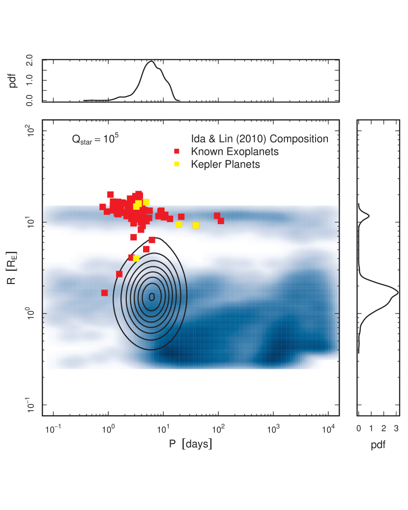
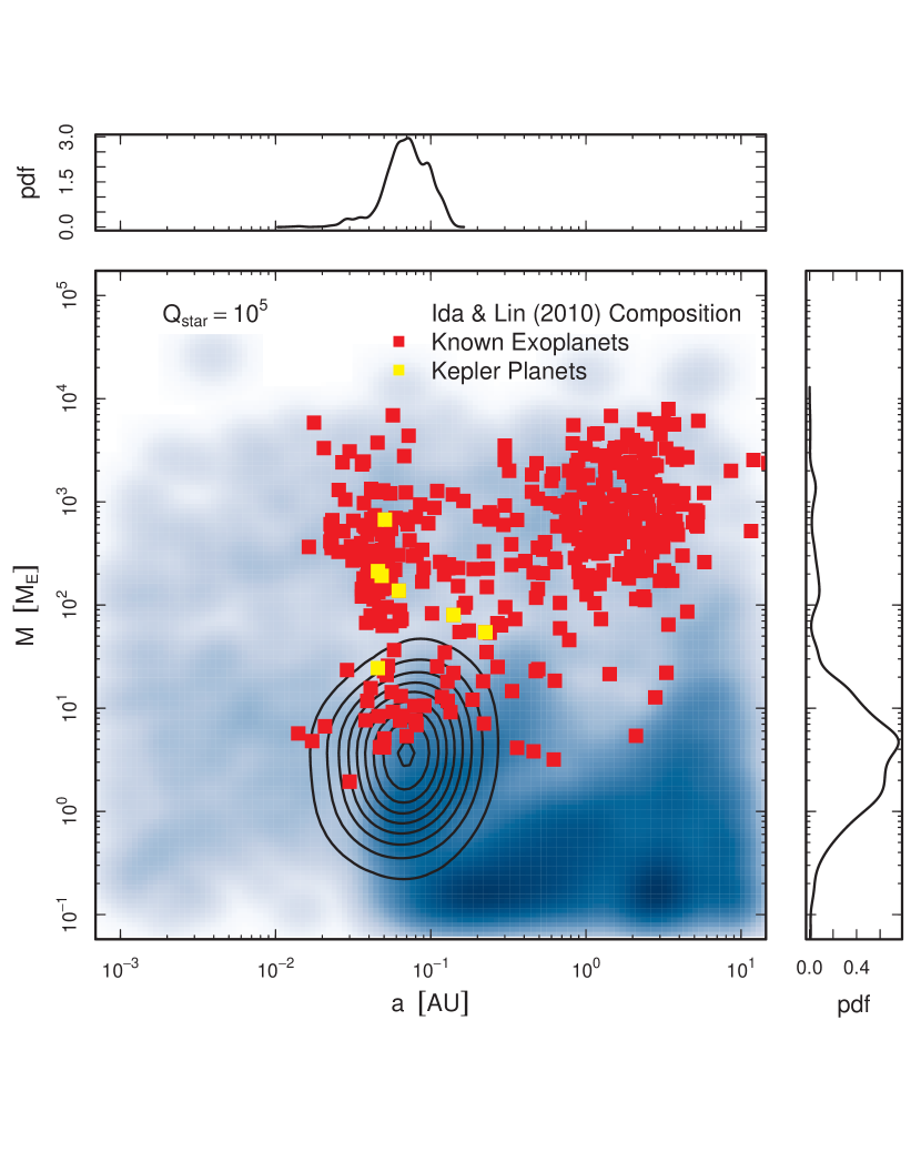
Figure 1.— Simulated Kepler observation of the extended IL10 EPS models assuming the mass–radius relation from Fortney et al. (2007) and strong tidal evolution (i.e., $Q_{\ast}^{\prime}=10^{5}$). The blue shading shows the underlying initial extended EPS before tidal evolution, while the black contours show the distribution of exoplanet properties including tidal evolution that would have been observable by Kepler in its first 43 days of science operation. We plot known exoplanets as red squares and confirmed Kepler planets as yellow squares. Left: Period–radius plane with marginal distributions. In this case, the orbits of giant planets quickly degrade due to strong tidal evolution. Right: Semimajor axis–mass plane with marginal distributions.

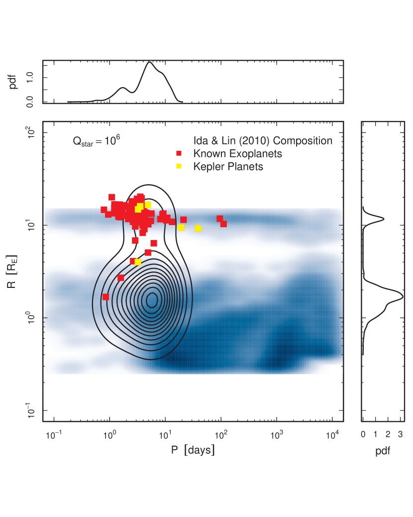
Figure 2.— Same as Figure 1 but assuming moderate tidal evolution (i.e., $Q_{\ast}^{\prime}=10^{6}$). In this case, the moderate tidal evolution allows some giant planets to survive.

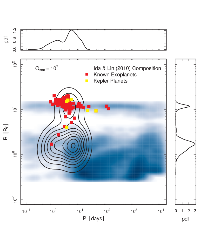
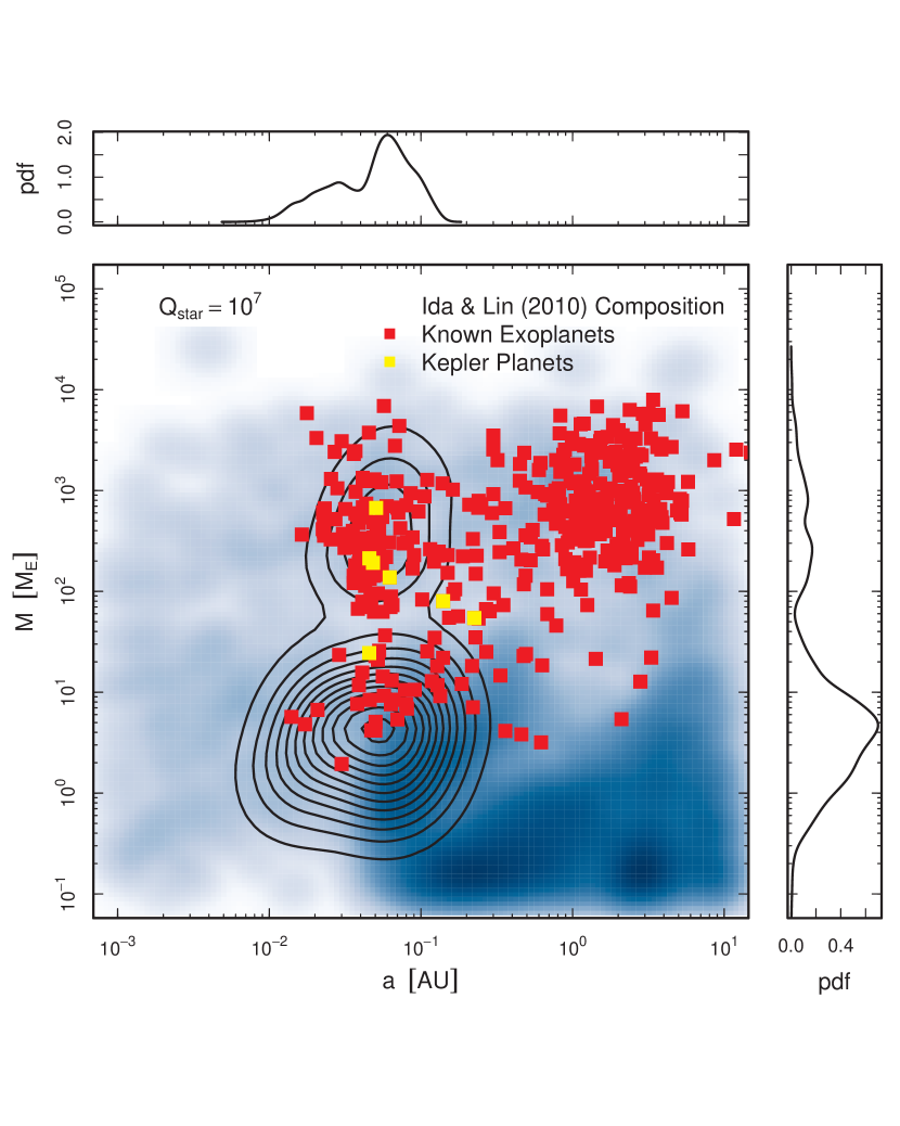
Figure 3.— Same as Figure 1 but assuming weak tidal evolution (i.e., $Q_{\ast}^{\prime}=10^{7}$). In this case, the weak tidal evolution allows many giant planets to survive. Interestingly, the observed period distribution of super-Earths extends to $P<1$ day, as super-Earths scattered to short-period orbits through dynamical interactions in multiple-planet systems would persist for a significant fraction of the main-sequence lifetime of their host stars. These very-hot super-Earths should occur in multiple-planet systems, and should preferentially orbit the least-dissipative host stars in the Kepler sample (i.e., those stars with $M_{\ast}\gtrsim 1.25~{}M_{\odot}$, convective cores, and radiative envelopes).

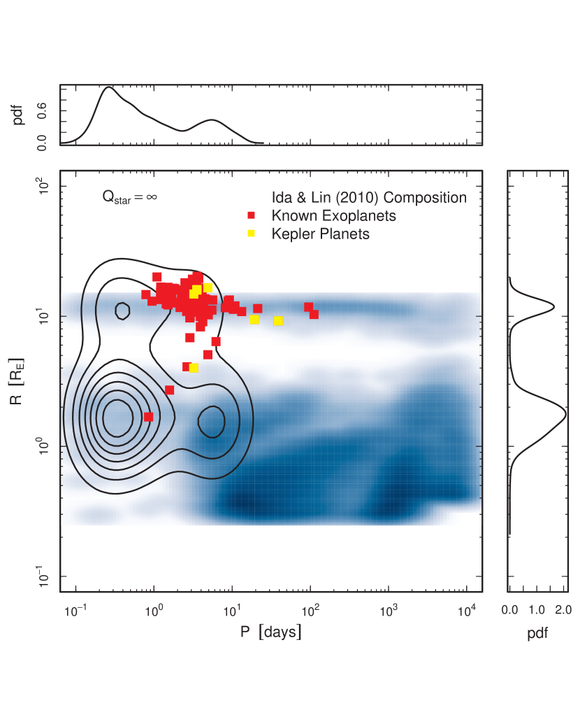
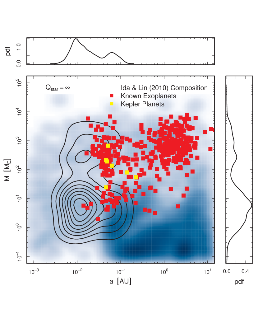
Figure 4.— Same as Figure 1 but assuming no tidal evolution (i.e., $Q_{\ast}^{\prime}=\infty$). In this case, the lack of tidal evolution allows all very-short period systems produced by dynamical interactions to survive.

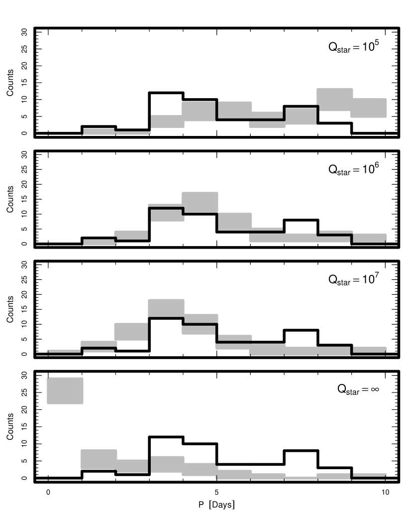
Figure 5.— Histograms describing the period distribution of short-period giant planets. The black curve represents the period distribution of short-period giant planets (e.g., planets with $R_{p}>0.5~{}R_{J}$ and $P<10$ days) from Borucki et al. (2010). The gray rectangles represent the one-sigma range in the period distribution of short-period giant planets (e.g., planets with $M_{p}>50~{}M_{\oplus}$ and $P<10$ days) expected from a Kepler-like observation of the extended IL10 EPS. Each panel corresponds to different assumptions for the strength of tidal evolution in the simulated Kepler observation of the extended IL10 EPS. Given the extended EPS, the first 43 days of Kepler science data already rule-out both strong tidal evolution and no tidal evolution; the current data favors $10^{6}\lesssim Q_{\ast}^{\prime}\lesssim 10^{7}$.

References

- Barker & Ogilvie (2009) Barker, A. J., & Ogilvie, G. I. 2009, MNRAS, 395, 2268
- Barker & Ogilvie (2010) Barker, A. J., & Ogilvie, G. I. 2010, MNRAS, 404, 1849
- Batalha et al. (2010a) Batalha, N. M., et al. 2010a, ApJ, 713, L103
- Batalha et al. (2010b) Batalha, N. M., et al. 2010b, ApJ, 713, L109
- Borucki et al. (2010) Borucki, W. J., et al. 2010, arXiv:1006.2799
- Bryson et al. (2010) Bryson, S. T., et al. 2010, ApJ, 713, L97
- Caldwell et al. (2010) Caldwell, D. A., et al. 2010, ApJ, 713, L92
- Dobbs-Dixon et al. (2004) Dobbs-Dixon, I., Lin, D. N. C., & Mardling, R. A. 2004, ApJ, 610, 464
- Ford et al. (2008) Ford, E. B., Quinn, S. N., & Veras, D. 2008, ApJ, 678, 1407
- Fortney et al. (2007) Fortney, J. J., Marley, M. S., & Barnes, J. W. 2007, ApJ, 659, 1661
- Gu et al. (2003) Gu, P.-G., Lin, D. N. C., & Bodenheimer, P. H. 2003, ApJ, 588, 509
- Haas et al. (2010) Haas, M. R., et al. 2010, ApJ, 713, L115
- Hatzes et al. (2010) Hatzes, A. P., et al. 2010, arXiv:1006.5476
- Ibgui & Burrows (2009) Ibgui, L., & Burrows, A. 2009, ApJ, 700, 1921
- Ida & Lin (2004) Ida, S., & Lin, D. N. C. 2004, ApJ, 604, 388
- Ida & Lin (2008) Ida, S., & Lin, D. N. C. 2008, ApJ, 685, 584
- Ida & Lin (2010) Ida, S., & Lin, D. N. C. 2010, ApJ, 719, 810
- Jackson et al. (2008a) Jackson, B., Greenberg, R., & Barnes, R. 2008a, ApJ, 678, 1396
- Jackson et al. (2008b) Jackson, B., Greenberg, R., & Barnes, R. 2008b, ApJ, 681, 1631
- Jackson et al. (2009) Jackson, B., Barnes, R., & Greenberg, R. 2009, ApJ, 698, 1357
- Jackson et al. (2010) Jackson, B., Miller, N., Barnes, R., Raymond, S. N., Fortney, J. J., & Greenberg, R. 2010, MNRAS, 1018
- Jenkins et al. (2010a) Jenkins, J. M., et al. 2010a, ApJ, 713, L87
- Jenkins et al. (2010b) Jenkins, J. M., et al. 2010b, ApJ, 713, L120
- Koch et al. (2010) Koch, D. G., et al. 2010, ApJ, 713, L79
- Léger et al. (2009) Léger, A., et al. 2009, A&A, 506, 287
- Levrard et al. (2009) Levrard, B., Winisdoerffer, C., & Chabrier, G. 2009, ApJ, 692, L9
- Li et al. (2010) Li, S.-L., Miller, N., Lin, D. N. C., & Fortney, J. J. 2010, Nature, 463, 1054
- Lin et al. (1996) Lin, D. N. C., Bodenheimer, P., & Richardson, D. C. 1996, Nature, 380, 606
- Mardling & Lin (2004) Mardling, R. A., & Lin, D. N. C. 2004, ApJ, 614, 955
- Masset et al. (2006) Masset, F. S., Morbidelli, A., Crida, A., & Ferreira, J. 2006, ApJ, 642, 478
- Miller et al. (2009) Miller, N., Fortney, J. J., & Jackson, B. 2009, ApJ, 702, 1413
- Mordasini et al. (2009a) Mordasini, C., Alibert, Y., & Benz, W. 2009a, A&A, 501, 1139
- Mordasini et al. (2009b) Mordasini, C., Alibert, Y., Benz, W., & Naef, D. 2009b, A&A, 501, 1161
- Ogihara et al. (2010) Ogihara, M., Duncan, M. J., & Ida, S. 2010, ApJ, 721, 1184
- Ogilvie & Lin (2004) Ogilvie, G. I., & Lin, D. N. C. 2004, ApJ, 610, 477
- Ogilvie & Lin (2007) Ogilvie, G. I., & Lin, D. N. C. 2007, ApJ, 661, 1180
- Pollack et al. (1996) Pollack, J. B., Hubickyj, O., Bodenheimer, P., Lissauer, J. J., Podolak, M., & Greenzweig, Y. 1996, Icarus, 124, 62
- Popper (1980) Popper, D. M. 1980, ARA&A, 18, 115
- Queloz et al. (2009) Queloz, D., et al. 2009, A&A, 506, 303
- Rasio et al. (1996) Rasio, F. A., Tout, C. A., Lubow, S. H., & Livio, M. 1996, ApJ, 470, 1187
- Reid & Hawley (2005) Reid, I. N., & Hawley, S. L. 2005, New Light on Dark Stars Red Dwarfs, Low-Mass Stars, Brown Stars, by I.N. Reid and S.L. Hawley. Springer-Praxis books in astrophysics and astronomy. Praxis Publishing Ltd, 2005. ISBN 3-540-25124-3
- Rocha-Pinto et al. (2000a) Rocha-Pinto, H. J., Scalo, J., Maciel, W. J., & Flynn, C. 2000a, ApJ, 531, L115
- Rocha-Pinto et al. (2000b) Rocha-Pinto, H. J., Scalo, J., Maciel, W. J., & Flynn, C. 2000b, A&A, 358, 869
- Sandquist et al. (1998) Sandquist, E., Taam, R. E., Lin, D. N. C., & Burkert, A. 1998, ApJ, 506, L65
- Schlaufman (2010) Schlaufman, K. C. 2010, ApJ, 719, 602
- Schlaufman et al. (2009) Schlaufman, K. C., Lin, D. N. C., & Ida, S. 2009, ApJ, 691, 1322
- Seager & Mallén-Ornelas (2003) Seager, S., & Mallén-Ornelas, G. 2003, ApJ, 585, 1038
- Ward (1997) Ward, W. R. 1997, Icarus, 126, 261
- Winn et al. (2010) Winn, J. N., Fabrycky, D., Albrecht, S., & Johnson, J. A. 2010, ApJ, 718, L145