Dynamical Polarizabilities of SU(3) Octet of Baryons
Abstract
We present calculations and an analysis of the spin-independent dipole electric and magnetic dynamical polarizabilities for the lowest in mass SU(3) octet of baryons. These extensive calculations are made possible by the recent implementation of semi-automatized calculations in Chiral Perturbation Theory which allows evaluating dynamical spin-independent electromagnetic polarizabilities from Compton scattering up to next-to-the-leading order. Our results are in good agreement with calculations performed for nucleons found in the literature. The dependencies for the range of photon energies up to , covering the majority of the meson photo production channels, are analyzed. The separate contributions into polarizabilities from the various baryon meson clouds are studied.
I Introduction
One of the ways to study the response of baryons to an external electromagnetic field is through Compton scattering, which allows us to extract fundamental response structure parameters, such as polarizabilities, and thus obtain information about the internal degrees of freedom. Electric () and magnetic () polarizabilities enter the effective Hamiltonian
| (1) |
and the induced electric ( and magnetic dipole moments, respectively, as response coefficients to the electric and magnetic fields. Their values, as well as some insight regarding which internal degrees of freedom of baryons define these values, can certainly shed more light on the internal structure of baryons. For instance, a positive or negative value of the magnetic polarizability already reflects whether a baryon has a paramagnetic or diamagnetic structure, respectively.
The nucleon polarizabilities have been addressed many times in the literature, but their evaluation still remains a challenging task for both theory and experiment. The world-average experimental values for the nucleon given in PDG are based on a very broad spectrum of experimental results. Theoretical predictions of the polarizabilities are also have a broad range of values and approaches Meissner ; BKM ; QCD ; PCQM ; Butler1993 . Since we are dealing with low-energy QCD here, we have no choice but rely on phenomenological approaches. In this paper, we chose an approach based on the effective chiral theory, Chiral Perturbation Theory (ChPT), where quark-gluon degrees of freedom are replaced by baryon-meson ones. The advantage of this approach is that it allows us to identify the sources responsible for shaping specific values of the polarizabilities by separately analyzing contributions from the baryon’s pion and kaon clouds. Baryon resonance excitations certainly have an impact as well, but since resonances enter into the calculations in the form of Rarita-Schwinger fields which complicate the calculations tremendously, we leave this for future projects. Although polarizabilities enter as the static coefficients in Eq.(1), we can expect that the baryon’s meson cloud could respond to the external electromagnetic field in a non-linear fashion so polarizabilities can depend on the energy of an incoming photon. The energy dependence of the dynamical polarizabilities is particularly visible at energies relevant to the various meson production channels. The main objective of this work is to study the impact of the baryon meson clouds on the electric and magnetic polarizabilities and analyze the energy dependence up to , covering the majority of the meson photo production channels.
The article is organized as follows. In Section II, we start with a brief outline of the formalism we use to describe the dynamics of the strong interactions, SU(3) ChPT, and our Computational Hadronic Model (CHM) which allowed us to semi-automatize calculations and thus expand applicability of ChPT. The details of the calculations of the Compton structure functions are shown in Section III. Numerical results along with the extensive analysis of the dynamical polarizabilities for the entire octet of baryons are shown in Section IV. Our findings are summarized in the conclusion (Section V).
II The Chiral Lagrangian and CHM
The Lagrangian describing the spontaneous symmetry breaking of due to the pseudo-Goldstone scalar bosons into is given by
| (2) |
which represents the first term of the effective Lagrangian from (Manohar1991, ), the only allowed term with two derivatives. Here, is the pion decay constant and the field is given by
| (3) |
where is the pseudo-Goldstone boson octet:
| (4) |
The covariant derivative is given by
| (5) |
where is the electromagnetic vector field potential and is the charge operator. The chiral symmetry transformation for the pseudo-Goldstone boson field is defined as . To introduce the baryon field into the effective Lagrangian uniquely, the new field is defined as . According to (Manohar1993, ), the chiral symmetry transformations for the field can be determined in a new basis as
| (6) |
The unitary matrix is implicitly defined from Eq.(6) in terms of and . Thus, the chiral transformation for the baryon field is unique, and chosen to be For the effective Lagrangian with baryons, this choice of basis is preferable because in this case pions have only derivative-type coupling. Consequently, the effective Lagrangian for the baryons can be written in terms of the vector field and the axial-vector field :
Following (Manohar1993, ), we take the leading-order baryon Lagrangian as
| (8) |
with an octet of baryons given by
| (9) |
and the covariant derivative defined as The strong coupling constants of the Lagrangian from Eq.(8) have been determined in (Manohar1991, ) to be and .
The effective Chiral Perturbation Theory of the strong interactions has been quite successful in the description of the hadronic interactions in the non-perturbative regime of QCD. Applying this theory towards Compton scattering, we can calculate all the necessary structure functions from the scattering amplitude and then extract the electromagnetic polarizabilities. However, to extract the polarizabilities successfully, according to the Low Energy Theorem (LET), we must include at least Next-to-the-Leading-Order (NLO) contributions. To deal with this rather non-trivial problem, one can either simplify calculations and include only the leading parts of the NLO contribution, or rely on some degree of automatization with computer-based packages. In this work, we employ the Computational Hadronic Model (CHM) which allows calculations to be completed up to NLO with the octet of mesons and baryons and the decuplet of resonances participating in the loop calculations. The renormalization is done using the Modified Minimal Subtraction scheme. CHM extends the FeynArts FeynArts package, designed for particles of the Standard Model only, into the hadronic sector, and can be used along with the FormCalc, LoopTools FormCalc and Form Form packages giving results first in analytical and then in numerical form. A more detailed description of CHM can be found in CHM .
III Compton Structure Functions
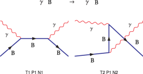
For a baryon without a structure, the Compton amplitude is derived from the Leading-Order (LO) perturbation expansion and is represented by the tree-level graphs (see Fig. (1)) by:
| (10) |
If we consider a baryon with structure, the spin-independent Compton scattering amplitude has the following form (Meissner, ):
| (11) |
Here, are the polarization vector, frequency and momenta of the incoming photon, respectively. Primed quantities denote the outgoing photon. The two structure constants and are the electric and magnetic polarizabilities of the baryon, correspondingly.
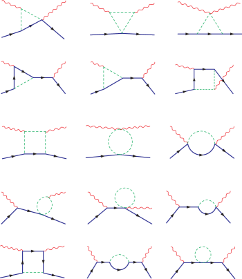
In order to satisfy the gauge invariance of the electromagnetic current this amplitude is not renormalized, and is expressed through the set of physical observables such as charge and mass. Recalling the well-known LET, in the Thomson limit (), the Compton amplitude in Eq.(11) should take the form of in Eq.(10). Hence, when soft photons are considered, the Compton scattering is sensitive only to the charge of the baryon and not to the internal structure. This means that the two structure constants, the electric and magnetic polarizabilities, can be determined only through the NLO loop calculations. A generic set of one-loop diagrams representing types of topologies allowed in Compton scattering is shown in Fig.(2). The full set of graphs includes crossed diagrams and wave function renormalization graphs absorbed into counterterms.
The polarizabilities in Eq.(11) are normally called static and defined in the limit of zero energy of the incoming photon, . However, the experiments providing their values were performed in the kinematic region of 55 to 800 MeV photons OL ; Galler ; GB . Thus, to determine the static polarizabilities by extrapolation to zero energy, one requires additional theoretical information about the energy dependence of the baryon’s structure parameters. To construct the energy dependence for the baryon polarizabilities, we follow the approach of H2 which offers an analysis of the dynamical polarizabilities in the energy domain up to the one-pion production threshold. Taking into account that polarizabilities in Eq.(11) now depend on the photon energy, we can rewrite the NLO Compton amplitude using the two energy-dependent structure functions and . For we have:
| (12) |
where is the photon’s scattering angle in the center of mass reference frame. Multipole expansion for the spin-independent structure functions implemented in H2 allows us to relate our computer-generated amplitude in the CHM to the dynamical electric and magnetic polarizabilities of the baryon. If we consider only dipole contributions in the multipole expansion of the structure functions, the two Compton structure functions of Eq.(12) read:
| (13) | |||||
Here, is the center of mass energy and is the mass of the baryon.
The Compton amplitude generated in the CHM is represented using the basis of the Dirac spinor chains. Our calculations are spin-independent, and the NLO amplitude takes the form of Eq.(12) after traces are taken. Simple extraction of the coefficients in front of and points to the structure functions and respectively.
Solving the system of Eq.[13] for using the zero momentum transfer approximation (), we obtain
| (14) | |||||
Although the CHM does produce analytic expressions for both structure functions, they are extremely lengthy and cumbersome and therefore are excluded from this article. Our results are presented in the form of numerical simulations of the dependencies of on photon energy in the next section.
IV Numerical Results
IV.1 Nucleon Polarizabilities
Since experimental results are only available for the nucleon, let us first provide an analysis of the polarizabilities of the neutron and proton. The world average values for the polarizabilities of the proton and neutron based on a broad spectrum of experimental values are given in PDG :
| (15) | |||||
Theoretical predictions of the polarizabilities also have a broad range of values and approaches (Meissner ; BKM ; QCD ; PCQM ; Butler1993 and references therein). For example, BKM who used the SU(2) Heavy Baryon to obtained the following:
| (16) |
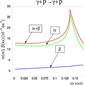
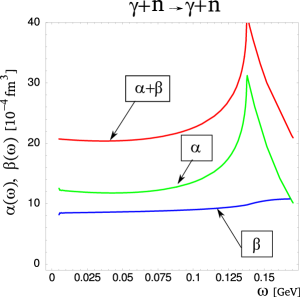
If we take for the mass of the pion and for the mass of the nucleon and extrapolate central values of the SU(3) dipole electric and magnetic polarizabilities to the zero photon energy (see Fig.(3)), we obtain:
| (17) |
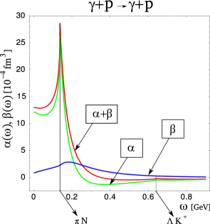
The uncertainties come from the uncertainties in the strong coupling constants and . Within these uncertainties, our results are in rather good agreement with the values of BKM .
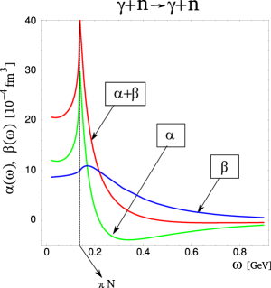
According to our calculations, the electric polarizability clearly shows a resonance-type structure at the pion production threshold, for both proton and neutron (see Fig.(3)). For the proton, there is a small additional peak at the energy defined by the kaon production threshold. The magnetic polarizability has a visible change in the slope at the pion production energy. As expected, all polarizabilities tend to go to zero (relaxation mechanism) with the growth of the photon energy. This can be explained by the fact that as the energy of the photon increases, the nucleon can no longer respond to the high-frequency external electromagnetic field.
As one can see from Fig.(4), is nearly constant for the energies up to , which means that in that range we can treat the electric polarizabilities as static. The dependencies given in Fig.(4) for the electric polarizabilities are in agreement with the result of H2 (which gives isoscalar values of the polarizabilities defined as an average between proton and neutron polarizabilities). Unlike the electric, the magnetic polarizability of the proton shows a relatively strong energy dependence. Ref. H2 shows similar behavior but our numerical results disagree. This can be explained by the fact that our calculations are completed in the framework of the ChPT model where the Next-to-NLO results may contribute. Additionally, we did not include any resonances, and, as was discussed in H1 ; Meissner ; BKM , resonance can have a sizable impact on the values of the magnetic polarizabilities. The detailed studies of the impact of the decuplet of resonances on the baryon polarizabilities will be a subject of our next work. For now, let us concentrate on finding out which specific degrees of freedom are responsible for such a dynamical behavior of the polarizabilities of the proton. The idea is to separate contributions coming from the diagrams with neutral pions and etas, charged pions, and kaons, which allows us to determine which of the proton meson clouds gives a dominant and defining contribution into the polarizabilities.
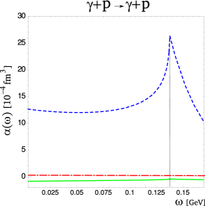
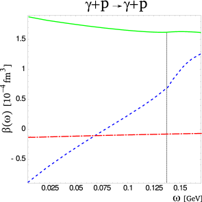
It is evident from Fig.(5) (left) that the charged pion cloud defines the dynamical behavior of the proton electric polarizability, and the neutral pion and kaon clouds do not have any impact. As for the magnetic polarizability, shown in Fig.(5) (right), dynamical behavior appears to be defined by the interplay between a relaxation mechanism coming from the neutral pion cloud and a rather strong excitation mechanism from the charged pion cloud. Although the positive value of the magnetic polarizability comes mostly from the neutral pions degree of freedom, the rapid increase of magnetic polarizability with energy is coming from the charged pions.
It is also interesting to observe that for the energy of the photon up to pion production threshold, the neutral pion cloud exhibits paramagnetic properties only. For the charged pion cloud, we observe diamagnetic behavior up to and a flip into paramagnetic behavior after that. Finally, the impact of the kaon cloud on the overall value of the magnetic polarizability is only static and almost negligible. We conclude that the dynamics of the pion clouds is most important and requires further analysis in different models.
IV.2 Polarizabilities of and
The dynamical dependence of the baryons electric and magnetic polarizabilities is summarized in Fig.(6).
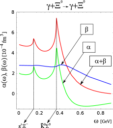
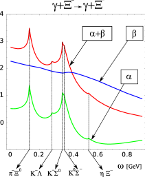
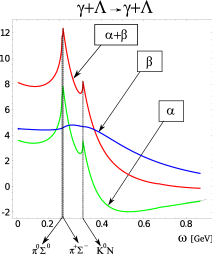
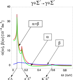
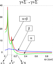
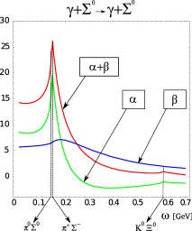
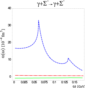
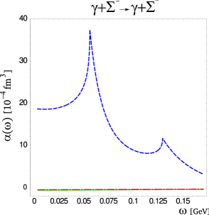
It is evident that for all baryons, the electric polarizabilities reflect various meson production channels in the form of the resonant behavior near a production threshold. The baryon magnetic polarizability shows different slope before and after the meson production threshold. Similar to the neutron, both polarizabilities of the neutral baryons are nearly constant for the energies up to the pion production threshold. Polarizabilities of the charged baryons have low-energy behavior similar to the proton, with almost constant electric and strongly variable magnetic polarizabilities. At low energies, the electric polarizabilities of and are the largest in the octet. They are completely defined by the contribution from the charged pions (see Fig.(7)). The total contribution into from kaons and neutral pions cancel each other completely. For , the overall contribution coming from those degrees of freedom is negative and reduces .
In addition, the magnetic polarizabilities of and dominate the electric for almost all photon energies up to . For , we observe the excitation mechanism which is similar to that earlier observed for the proton in magnetic polarizability. On the contrary, the magnetic polarizability of shows a strong relaxation behavior. To understand the cause of the overall negative slope in magnetic polarizability of the cascade, let us use the same approach as before and show explicitly the contributions coming from kaons, neutral pions, and charged pions.
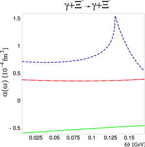
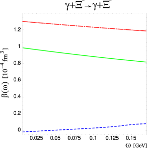
As one can see from Fig.(8), for the electric polarizability, the contribution coming from kaons almost completely cancels out the neutral pion contribution, leaving the final result defined by the charged pion cloud. As for the cascade magnetic polarizability, contributions coming from the kaon and neutral pion degrees of freedom are the dominant ones, and as a result they define the overall behavior of the magnetic polarizability. The small contribution from the charged pions is suppressed, although it shows an excitation mechanism similar to that of the proton. Similarly, we observe a flip from diamagnetic to paramagnetic behavior around an energy of .
At this point it is interesting to compare our results with those obtained in other models. Table 1 shows our results for the dynamical electric and magnetic hyperon polarizabilities extrapolated to zero photon energy.
| B | ||
|---|---|---|
| 2.1 | 2.8 | |
| 3.7 | 4.5 | |
| 8.6 | 5.7 | |
| 0.5 | 2.3 | |
| 17.1 | 0.7 | |
| 17.4 | 1.9 |
Table 1. The CHM predictions for the static electric and magnetic polarizabilities of hyperons in units of .
Calculations of the static electromagnetic polarizabilities of hyperons were performed in several models by NRQM1 ; NRQM2 ; MeissnerHB ; Soliton ; QCD_SUM ; LargeNC and give a rather broad spectrum of predictions. Our calculations show a rather large electric polarizability for which is in agreement with the non-relativistic quark model NRQM NRQM1 ; NRQM2 results. However, for baryon, we have almost identical (slightly larger) value of which clearly disagrees with findings of NRQM1 ; NRQM2 there is much smaller. In general, calculations done in MeissnerHB ; Soliton ; QCD_SUM ; LargeNC predict larger value for comparing to but with substantially smaller splitting arising from the kaon contribution.
As it was mentioned in LargeNC and confirmed by our calculations, the overall value of electric polarizabilities strongly depend on the hyperon mass splitting. It is interesting to see how our results for the will change if we remove the sigma hyperon mass splitting. We expect that in this case, the charged pion contributions into will be exactly the same, with kaon and neutral pions clouds defining the overall outcome of the splitting and leading to the smaller value of the . Explicitly, without the hyperon mass splitting, we find that and which gives and restores ordering of these polarizabilities. At the moment, there is no experimental data available on the polarizabilities of sigma hyperons, but hopefully future experiments will help to clarify the situation.
Since the SU(3) extension of HBChPT in MeissnerHB operates in the heavy-baryon limit with the same symmetries of the SU(3) Lagrangian as in ChPT, we find it interesting to compare our results for the electric polarizabilities with MeissnerHB . For the neutral baryons, we observe comparable magnitude and the same ordering of electric polarizabilities as in MeissnerHB : , confirming that decreases with the increase of of the baryon strangeness. As for the charged baryons, we find , in contrast to MeissnerHB . Clearly, the electric polarizabilities for the sigma hyperons are quite different and require further studies. We plan to work in this direction by attempting two-loop calculations and including resonance excitations.
V Conclusion
We applied the Computational Hadronic Model for Compton scattering and calculated spin-independent dipole electric and magnetic dynamical polarizabilities for the SU(3) set of baryons. The dependence of the dynamical polarizabilities on the photon energies up to covers the majority of the meson photo production channels.
The electric polarizability has resonant-type behavior near meson production thresholds. The magnetic polarizability shows a change of slope at the production energy. Unlike electric, magnetic polarizability exhibited strong low-energy dependence for all charged baryons. Neutral baryons show very little low-energy dependence and hence their polarizabilities can be treated as a static.
The study of the separate contributions into polarizabilities coming from the various baryon meson clouds proved to be interesting. For the proton and the charged sigma baryons, the magnetic polarizability has a strong excitation mechanism and is driven by the charged pion cloud. For the charged cascade baryon, we find the relaxation mechanism in magnetic polarizability explained by the dominant impact coming from the kaon and neutral pion clouds. In general, we find that neutral pions define the overall paramagnetic behavior in the magnetic polarizabilities for all baryons. For the charged pion clouds, magnetic polarizability starts as a diamagnetic type and then flips to paramagnetic behavior at the range of photon energies.
Apparently the physics of the dynamical polarizabilities, in addition to resonance excitations, is driven by the dynamics of the separate meson clouds. Experimental studies of these dependencies would help us to understand baryon intrinsic degrees of freedom. From the experiment point of view, the best tool in the studies of the internal baryon dynamics is offered through Virtual Compton Scattering (VCS), which includes polarized-target experiments on nucleons in the forward/backward direction and offers an excellent way to study spin structure parameters of the nucleon. These experiments would require the calculations of the spin-dependent dynamical polarizabilities. For the static spin-dependent polarizabilities, calculations within ChPT were completed by Ref.HHKK . We believe that with the CHM, calculations of the spin-dependent dynamical polarizabilities should be possible in the near future.
Although our calculations are done for NLO only, they still generated an interesting set of results for the dynamical polarizabilities. However, due to the well-known inconsistency of ChPT in power counting, it is highly desirable to perform the Next-to-NLO calculations as well. That would determine the convergence of the perturbative series and hence provide better understanding of the internal baryons dynamics.
The ChPT gives a systematic prescription on how to incorporate baryon resonances, but we leave the problem out of this paper. A detailed analysis of the impact of the and other resonances on the electromagnetic polarizabilities will be a subject of our future studies.
VI Acknowledgment
This work has been supported by NSERC. The authors would like to thank T. Hahn for making packages such as FeynArts, FormCalc and LoopTools available to the physics community. A.A. is grateful to M. Butler for inspiring discussion regarding Chiral Perturbation Theory.
References
- (1) C. Amsler et al., Phys. Lett. B667, (2008).
- (2) V. Bernard, N. Kaiser and U.-G. Meisner, BUTP-91/30, (1991); Nucl. Phys. B373:346-370, (1992).
- (3) V. Bernard, N. Kaiser, A. Schmidt and U.-G. Meissner, Phys. Lett. B319 269 (1993).
- (4) F. Lee et al., Phys. Rev. D73 034503, (2006).
- (5) Y. Dong et al., J. Phys. G: Nucl. Part. Phys. 32 203-220, (2006).
- (6) M. N. Butler, M. J. Savage and R. P. Springer, Nucl. Phys. B399 69, (1993).
- (7) E. Jenkins and A. Manohar, UCSD/PTH 91-30, (1991).
- (8) A. Manohar, hep-ph/9305298 (1993).
- (9) T. Hahn, Comput. Phys. Commun. 140 418 [hep-ph/0012260] (2001).
- (10) T. Hahn, M. Perez-Victoria, Comput. Phys. Commun. 118 153 [hep-ph/9807565] (1999).
- (11) J. A. M. Vermaseren, math-ph/0010025, (2000).
- (12) A. Aleksejevs and M. Butler, J. Phys. G 37 (2010).
- (13) V. Olmos de Leon et al., Eur. Phys. J. A10 207, (2001).
- (14) G. Galler et al., Phys. Lett. B503 245, nucl-ex/0102003, (2001).
- (15) G. Blanpied et al., Phys. Rev. C64 025203, (2001).
- (16) H. Griehammer and T. Hemmert, Phys. Rev. C65 045207, (2002).
- (17) T. Hemmert, B. Holstein and J. Kambor, Phys. Rev. D55 5598, (1997).
- (18) T. Hemmert, B. Holstein, J. Kambor and G. Knochlein , Phys. Rev. D57 5746, (1998).
- (19) A. Denner, S. Dittmaier and T. Hahn, Phys. Rev. D56 117, hep-ph/9612390, (1997).
- (20) A. Denner and T. Hahn, Nucl. Phys. B525 27, (hep-ph/9711302), (1998) .
- (21) W. Beenakker and A. Denner, Int. J. Mod. Phys. A9 4837, (1994) .
- (22) T. Hahn, hep-ph/0007062, (2001).
- (23) W. Hollik and C. Schappacher, Nucl. Phys. B545 98, hep-ph/9807427, (1999).
- (24) J. Guasch, W. Hollik, and A. Kraft, Nucl. Phys. B596 66, hep-ph/9911452, (2001).
- (25) V. A. Petrunkin, Sov. J. Part. Nucl. 12 278 (1981).
- (26) H. J. Lipkin, M. A. Moinester, Phys. Lett. B 287 179 (1992).
- (27) V. Bernard, N. Kaiser, J. Kambor, U. -G. Meissner, Phys. Rev. D 46 2756 (1992).
- (28) C. Gobbi, C. Schat, N. Scoccola, Nucl. Phys. A598 318-334 (1996).
- (29) T. Nishikawa, S. Saito, Y. Kondo, Phys. Lett. B422 26-32 (1998).
- (30) Y. Tanushi, S. Saito, M. Uehara, Phys. Rev. C61 055204 (2000).