On the representation theory of finite $\mathcal{J}$-trivial monoids

Abstract.

In 1979, Norton showed that the representation theory of the $0$-Hecke algebra admits a rich combinatorial description. Her constructions rely heavily on some triangularity property of the product, but do not use explicitly that the $0$-Hecke algebra is a monoid algebra.

The thesis of this paper is that considering the general setting of monoids admitting such a triangularity, namely $\mathcal{J}$-trivial monoids, sheds further light on the topic. This is a step in an ongoing effort to use representation theory to automatically extract combinatorial structures from (monoid) algebras, often in the form of posets and lattices, both from a theoretical and computational point of view, and with an implementation in Sage.

Motivated by ongoing work on related monoids associated to Coxeter systems, and building on well-known results in the semi-group community (such as the description of the simple modules or the radical), we describe how most of the data associated to the representation theory (Cartan matrix, quiver) of the algebra of any $\mathcal{J}$-trivial monoid $M$ can be expressed combinatorially by counting appropriate elements in $M$ itself. As a consequence, this data does not depend on the ground field and can be calculated in $O(n^{2})$, if not $O(nm)$, where $n=|M|$ and $m$ is the number of generators. Along the way, we construct a triangular decomposition of the identity into orthogonal idempotents, using the usual Möbius inversion formula in the semi-simple quotient (a lattice), followed by an algorithmic lifting step.

Applying our results to the $0$-Hecke algebra (in all finite types), we recover previously known results and additionally provide an explicit labeling of the edges of the quiver. We further explore special classes of $\mathcal{J}$-trivial monoids, and in particular monoids of order preserving regressive functions on a poset, generalizing known results on the monoids of nondecreasing parking functions.

1. Introduction

The representation theory of the $0$-Hecke algebra (also called degenerate Hecke algebra) was first studied by P.-N. Norton [Nor79] in type A and expanded to other types by Carter [Car86]. Using an analogue of Young symmetrizers, they describe the simple and indecomposable projective modules together with the Cartan matrix. An interesting combinatorial application was then found by Krob and Thibon [KT97] who explained how induction and restriction of these modules gives an interpretation of the products and coproducts of the Hopf algebras of noncommutative symmetric functions and quasi-symmetric functions. Two other important steps were further made by Duchamp–Hivert–Thibon [DHT02] for type $A$ and Fayers [Fay05] for other types, using the Frobenius structure to get more results, including a description of the Ext-quiver. More recently, a family of minimal orthogonal idempotents was described in [Den10a, Den10b]. Through divided difference (Demazure operator), the $0$-Hecke algebra has a central role in Schubert calculus and also appeared has connection with $K$-theory [Dem74, Las01, Las04, Mil05, BKS⁺08, LSS10].

Like several algebras whose representation theory was studied in recent years in the algebraic combinatorics community (such as degenerated left regular bands, Solomon-Tits algebras, …), the $0$-Hecke algebra is the algebra of a finite monoid endowed with special properties. Yet this fact was seldom used (including by the authors), despite a large body of literature on finite semi-groups, including representation theory results [Put96, Put98, Sal07, Sal08, MS08, Sch08, Ste06, Ste08, AMV05, AMSV09, GMS09, IRS10]. From these, one can see that much of the representation theory of a semi-group algebra is combinatorial in nature (provided the representation theory of groups is known). One can expect, for example, that for aperiodic semi-groups (which are semi-groups which contain only trivial subgroups) most of the numerical information (dimensions of the simple/projective indecomposable modules, induction/restriction constants, Cartan matrix) can be computed without using any linear algebra. In a monoid with partial inverses, one finds (non-trivial) local groups and an understanding of the representation theory of these groups is necessary for the full representation theory of the monoid. In this sense, the notion of aperiodic monoids is orthogonal to that of groups as they contain only trivial group-like structure (there are no elements with partial inverses). On the same token, their representation theory is orthogonal to that of groups.

The main goal of this paper is to complete this program for the class of $\mathcal{J}$-trivial monoids (a monoid $M$ is $\mathcal{J}$-trivial provided that there exists a partial ordering $\leq$ on $M$ such that for all $x,y\in M$, one has $xy\leq x$ and $xy\leq y$). In this case, we show that most of the combinatorial data of the representation theory, including the Cartan matrix and the quiver can be expressed by counting particular elements in the monoid itself. A second goal is to provide a self-contained introduction to the representation theory of finite monoids, targeted at the algebraic combinatorics audience, and focusing on the simple yet rich case of $\mathcal{J}$-trivial monoids.

The class of $\mathcal{J}$-trivial monoids is by itself an active subject of research (see e.g. [ST88, HP00, Ver08]), and contains many monoids of interest, starting with the $0$-Hecke monoid. Another classical $\mathcal{J}$-trivial monoid is that of nondecreasing parking functions, or monoid of order preserving regressive functions on a chain. Hivert and Thiéry [HT06, HT09] showed that it is a natural quotient of the $0$-Hecke monoid and used this fact to derive its complete representation theory. It is also a quotient of Kiselman’s monoid which is studied in [KM09] with some representation theory results. Ganyushkin and Mazorchuk [GM10] pursued a similar line with a larger family of quotients of both the $0$-Hecke monoid and Kiselman’s monoid.

The extension of the program to larger classes of monoids, like $\mathcal{R}$-trivial or aperiodic monoids, is the topic of a forthcoming paper. Some complications necessarily arise since the simple modules are not necessarily one-dimensional in the latter case. The approach taken there is to suppress the dependence upon specific properties of orthogonal idempotents. Following a complementary line, Berg, Bergeron, Bhargava, and Saliola [BBBS10] have very recently provided a construction for a decomposition of the identity into orthogonal idempotents for the class of $\mathcal{R}$-trivial monoids.

The paper is arranged as follows. In Section 2 we recall the definition of a number of classes of monoids, including the $\mathcal{J}$-trivial monoids, define some running examples of $\mathcal{J}$-trivial monoids, and establish notation.

In Section 3 we establish the promised results on the representation theory of $\mathcal{J}$-trivial monoids, and illustrates them on several examples including the $0$-Hecke monoid. We describe the radical, construct combinatorial models for the projective and simple modules, give a lifting construction to obtain orthogonal idempotents, and describe the Cartan matrix and the quiver, with an explicit labelling of the edges of the latter. We briefly comment on the complexity of the algorithms to compute the various pieces of information, and their implementation in Sage. All the constructions and proofs involve only combinatorics in the monoid or linear algebra with unitriangular matrices. Due to this, the results do not depend on the ground field $\mathbb{K}$. In fact, we have checked that all the arguments pass to $\mathbb{K}=\mathbb{Z}$ and therefore to any ring (note however that the definition of the quiver that we took comes from [ARO97], where it is assumed that $\mathbb{K}$ is a field). It sounds likely that the theory would apply mutatis-mutandis to semi-rings, in the spirit of [IRS10].

Finally, in Section 4, we examine the monoid of order preserving regressive functions on a poset $P$, which generalizes the monoid of nondecreasing parking functions on the set $\{1,\ldots,N\}$. We give combinatorial constructions for idempotents in the monoid and also prove that the Cartan matrix is upper triangular. In the case where $P$ is a meet semi-lattice (or, in particular, a lattice), we establish an idempotent generating set for the monoid, and present a conjectural recursive formula for orthogonal idempotents in the algebra.

1.1. Acknowledgments

We would like to thank Chris Berg, Nantel Bergeron, Sandeep Bhargava, Sara Billey, Jean-Éric Pin, Franco Saliola, and Benjamin Steinberg for enlightening discussions. We would also like to thank the referee for detailed reading and many remarks that improved the paper. This research was driven by computer exploration, using the open-source mathematical software Sage [S⁺09] and its algebraic combinatorics features developed by the Sage-Combinat community [SCc08], together with the Semigroupe package by Jean-Éric Pin [Pin10b].

TD and AS would like to thank the Université Paris Sud, Orsay for hospitality. NT would like to thank the Department of Mathematics at UC Davis for hospitality. TD was in part supported by NSF grants DMS–0652641, DMS–0652652, by VIGRE NSF grant DMS–0636297, and by a Chateaubriand fellowship from the French Embassy in the US. FH was partly supported by ANR grant 06-BLAN-0380. AS was in part supported by NSF grants DMS–0652641, DMS–0652652, and DMS–1001256. NT was in part supported by NSF grants DMS–0652641, DMS–0652652.

2. Background and Notation

A monoid is a set $M$ together with a binary operation $\cdot:M\times M\to M$ such that we have closure ($x\cdot y\in M$ for all $x,y\in M$), associativity ( $(x\cdot y)\cdot z=x\cdot(y\cdot z)$ for all $x,y,z\in M$), and the existence of an identity element $1\in M$ (which satistfies $1\cdot x=x\cdot 1=x$ for all $x\in M$). In this paper, unless explicitly mentioned, all monoids are finite. We use the convention that $A\subseteq B$ denotes $A$ a subset of $B$, and $A\subset B$ denotes $A$ a proper subset of $B$.

Monoids come with a far richer diversity of features than groups, but collections of monoids can often be described as varieties satisfying a collection of algebraic identities and closed under subquotients and finite products (see e.g. [Pin86, Pin10a] or [Pin10a, Chapter VII]). Groups are an example of a variety of monoids, as are all of the classes of monoids described in this paper. In this section, we recall the basic tools for monoids, and describe in more detail some of the varieties of monoids that are relevant to this paper. A summary of those is given in Figure 1.

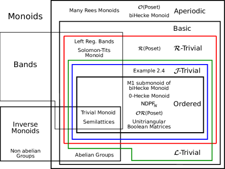
Figure 1. Classes of finite monoids, with examples

In 1951 Green introduced several preorders on monoids which are essential for the study of their structures (see for example [Pin10a, Chapter V]). Let $M$ be a monoid and define $\leq_{\mathcal{R}},\leq_{\mathcal{L}},\leq_{\mathcal{J}},\leq_{\mathcal{H}}$ for $x,y\in M$ as follows:

$$\begin{split}&x\leq_{\mathcal{R}}y\quad\text{if and only if $x=yu$ for some $u\in M$}\\ &x\leq_{\mathcal{L}}y\quad\text{if and only if $x=uy$ for some $u\in M$}\\ &x\leq_{\mathcal{J}}y\quad\text{if and only if $x=uyv$ for some $u,v\in M$}\\ &x\leq_{\mathcal{H}}y\quad\text{if and only if $x\leq_{\mathcal{R}}y$ and $x\leq_{\mathcal{L}}y$.}\end{split}$$

These preorders give rise to equivalence relations:

$$\begin{split}&x\;\mathcal{R}\;y\quad\text{if and only if $xM=yM$}\\ &x\;\mathcal{L}\;y\quad\text{if and only if $Mx=My$}\\ &x\;\mathcal{J}\;y\quad\text{if and only if $MxM=MyM$}\\ &x\;\mathcal{H}\;y\quad\text{if and only if $x\;\mathcal{R}\;y$ and $x\;\mathcal{L}\;y$.}\end{split}$$

We further add the relation $\leq_{\mathcal{B}}$ (and its associated equivalence relation $\mathcal{B}$) defined as the finest preorder such that $x\leq_{\mathcal{B}}1$, and

(2.1) $$x\leq_{\mathcal{B}}y uxv\leq_{\mathcal{B}}uyv x,y,u,v\in M$$ implies that for all .

(One can view $\leq_{\mathcal{B}}$ as the intersection of all preorders with the above property; there exists at least one such preorder, namely $x\leq y$ for all $x,y\in M$).

Beware that $1$ is the largest element of these (pre)-orders. This is the usual convention in the semi-group community, but is the converse convention from the closely related notions of left/right/Bruhat order in Coxeter groups.

Definition 2.1.

A monoid $M$ is called $\mathcal{K}$-trivial if all $\mathcal{K}$-classes are of cardinality one, where $\mathcal{K}\in\{\mathcal{R},\mathcal{L},\mathcal{J},\mathcal{H},\mathcal{B}\}$.

An equivalent formulation of $\mathcal{K}$-triviality is given in terms of ordered monoids. A monoid $M$ is called:

right ordered if $$xy\leq x x,y\in M$$ for all

left ordered if $$xy\leq y x,y\in M$$ for all

left-right ordered if $$xy\leq x xy\leq y x,y\in M$$ and for all

two-sided ordered if $$xy=yz\leq y x,y,z\in M xy=yz$$ for all with

ordered with $$1 x\leq 1 x\in M x\leq y$$ on top if for all , and

implies $$uxv\leq uyv x,y,u,v\in M$$ for all

for some partial order $\leq$ on $M$.

Proposition 2.2.

$M$ is right ordered (resp. left ordered, left-right ordered, two-sided ordered, ordered with $1$ on top) if and only if $M$ is $\mathcal{R}$-trivial (resp. $\mathcal{L}$-trivial, $\mathcal{J}$-trivial, $\mathcal{H}$-trivial, $\mathcal{B}$-trivial).

When $M$ is $\mathcal{K}$-trivial for $\mathcal{K}\in\{\mathcal{R},\mathcal{L},\mathcal{J},\mathcal{H},\mathcal{B}\}$, then $\leq_{\mathcal{K}}$ is a partial order, called $\mathcal{K}$-order. Furthermore, the partial order $\leq$ is finer than $\leq_{\mathcal{K}}$: for any $x,y\in M$, $x\leq_{\mathcal{K}}y$ implies $x\leq y$.

Proof.

We give the proof for right-order as the other cases can be proved in a similar fashion.

Suppose $M$ is right ordered and that $x,y\in M$ are in the same $\mathcal{R}$-class. Then $x=ya$ and $y=xb$ for some $a,b\in M$. This implies that $x\leq y$ and $y\leq x$ so that $x=y$.

Conversely, suppose that all $\mathcal{R}$-classes are singletons. Then $x\leq_{\mathcal{R}}y$ and $y\leq_{\mathcal{R}}x$ imply that $x=y$, so that the $\mathcal{R}$-preorder turns into a partial order. Hence $M$ is right ordered using $xy\leq_{\mathcal{R}}x$. ∎

2.1. Aperiodic and $\mathcal{R}$-trivial monoids

The class of $\mathcal{H}$-trivial monoids coincides with that of aperiodic monoids (see for example [Pin10a, Proposition 4.9]): a monoid is called aperiodic if for any $x\in M$, there exists some positive integer $N$ such that $x^{N}=x^{N+1}$. The element $x^{\omega}:=x^{N}=x^{N+1}=x^{N+2}=\cdots$ is then an idempotent (the idempotent $x^{\omega}$ can in fact be defined for any element of any monoid [Pin10a, Chapter VI.2.3], even infinite monoids; however, the period $k$ such that $x^{N}=x^{N+k}$ need no longer be $1$). We write $E(M):=\{x^{\omega}\mid x\in M\}$ for the set of idempotents of $M$.

Our favorite example of a monoid which is aperiodic, but not $\mathcal{R}$-trivial, is the biHecke monoid studied in [HST10a, HST10b]. This is the submonoid of functions from a finite Coxeter group $W$ to itself generated simultaneously by the elementary bubble sorting and antisorting operators $\overline{\pi}_{i}$ and $\pi_{i}$

(2.2) $$M(W):=\langle\pi_{1},\pi_{2},\ldots,\pi_{n},\overline{\pi}_{1},\overline{\pi}_{2},\ldots,\overline{\pi}_{n}\rangle\,.$$

See [HST10a, Definition 1.1] and [HST10a, Proposition 3.8].

The smaller class of $\mathcal{R}$-trivial monoids coincides with the class of so-called weakly ordered monoids as defined by Schocker [Sch08]. Also, via the right regular representation, any $\mathcal{R}$-trivial monoid can be represented as a monoid of regressive functions on some finite poset $P$ (a function $f:P\to P$ is called regressive if $f(x)\leq x$ for every $x\in P$); reciprocally any such monoid is $\mathcal{R}$-trivial. We now present an example of a monoid which is $\mathcal{R}$-trivial, but not $\mathcal{J}$-trivial.

Example 2.3.

Take the free left regular band $\mathcal{B}$ generated by two idempotents $a,b$. Multiplication is given by concatenation taking into account the idempotent relations, and then selecting only the two left factors (see for example [Sal07]). So $\mathcal{B}=\{1,a,b,ab,ba\}$ and $1\mathcal{B}=\mathcal{B}$, $a\mathcal{B}=\{a,ab\}$, $b\mathcal{B}=\{b,ba\}$, $ab\mathcal{B}=\{ab\}$, and $ba\mathcal{B}=\{ba\}$. This shows that all $\mathcal{R}$-classes consist of only one element and hence $\mathcal{B}$ is $\mathcal{R}$-trivial.

On the other hand, $\mathcal{B}$ is not $\mathcal{L}$-trivial since $\{ab,ba\}$ forms an $\mathcal{L}$-class since $b\cdot ab=ba$ and $a\cdot ba=ab$. Hence $\mathcal{B}$ is also not $\mathcal{J}$-trivial.

2.2. $\mathcal{J}$-trivial monoids

The most important for our paper is the class of $\mathcal{J}$-trivial monoids. In fact, our main motivation stems from the fact that the submonoid $M_{1}=\{f\in M\mid f(1)=1\}$ of the biHecke monoid $M$ in (2.2) of functions that fix the identity, is $\mathcal{J}$-trivial (see [HST10a, Corollary 4.2] and [HST10b]).

Example 2.4.

The following example of a $\mathcal{J}$-trivial monoid is given in [ST88]. Take $M=\{1,x,y,z,0\}$ with relations $x^{2}=x$, $y^{2}=y$, $xz=zy=z$, and all other products are equal to $0$. Then $M1M=M$, $MxM=\{x,z,0\}$, $MyM=\{y,z,0\}$, $MzM=\{z,0\}$, and $M0M=\{0\}$, which shows that $M$ is indeed $\mathcal{J}$-trivial. Note also that $M$ is left-right ordered with the order $1>x>y>z>0$, which by Proposition 2.2 is equivalent to $\mathcal{J}$-triviality.

2.3. Ordered monoids (with $1$ on top)

Ordered monoids $M$ with $1$ on top form a subclass of $\mathcal{J}$-trivial monoids. To see this suppose that $x,y\in M$ are in the same $\mathcal{R}$-class, that is $x=ya$ and $y=xb$ for some $a,b\in M$. Since $a\leq 1$, this implies $x=ya\leq y$ and $y=xb\leq x$ so that $x=y$. Hence $M$ is $\mathcal{R}$-trivial. By analogous arguments, $M$ is also $\mathcal{L}$-trivial. Since $M$ is finite, this implies that $M$ is $\mathcal{J}$-trivial (see [Pin10a, Chapter V, Theorem 1.9]).

The next example shows that ordered monoids with 1 on top form a proper subclass of $\mathcal{J}$-trivial monoids.

Example 2.5.

The monoid $M$ of Example 2.4 is not ordered. To see this suppose that $\leq$ is an order on $M$ with maximal element $1$. The relation $y\leq 1$ implies $0=z^{2}\leq z=xzy\leq xy=0$ which contradicts $z\neq 0$.

It was shown by Straubing and Thérien [ST88] and Henckell and Pin [HP00] that every $\mathcal{J}$-trivial monoid is a quotient of an ordered monoid with $1$ on top.

In the next two subsections we present two important examples of ordered monoids with $1$ on top: the $0$-Hecke monoid and the monoid of regressive order preserving functions, which generalizes nondecreasing parking functions.

2.4. $0$-Hecke monoids

Let $W$ be a finite Coxeter group. It has a presentation

(2.3) $$W=\langle\,s_{i}\;\text{for}\;i\in I\ \mid\ (s_{i}s_{j})^{m(s_{i},s_{j})},\ \forall i,j\in I\,\rangle\,,$$

where $I$ is a finite set, $m(s_{i},s_{j})\in\{1,2,\dots,\infty\}$, and $m(s_{i},s_{i})=1$. The elements $s_{i}$ with $i\in I$ are called simple reflections, and the relations can be rewritten as:

(2.4) $$s_{i}^{2} =1 \text{ for all $i\in I$}\,,$$

$$\underbrace{s_{i}s_{j}s_{i}s_{j}s_{i}\cdots}_{m(s_{i},s_{j})} =\underbrace{s_{j}s_{i}s_{j}s_{i}s_{j}\cdots}_{m(s_{i},s_{j})} \text{ for all $i,j\in I$}\,,$$

where $1$ denotes the identity in $W$. An expression $w=s_{i_{1}}\cdots s_{i_{\ell}}$ for $w\in W$ is called reduced if it is of minimal length $\ell$. See [BB05, Hum90] for further details on Coxeter groups.

The Coxeter group of type $A_{n-1}$ is the symmetric group ${\mathfrak{S}_{n}}$ with generators $\{s_{1},\dots,s_{n-1}\}$ and relations:

(2.5) $$s_{i}^{2} =1 \text{ for }1\leq i\leq n-1\,,$$

$$s_{i}s_{j} =s_{j}s_{i} \text{ for }|i-j|\geq 2\,,$$

$$s_{i}s_{i+1}s_{i} =s_{i+1}s_{i}s_{i+1} \text{ for }1\leq i\leq n-2\,;$$

the last two relations are called the braid relations.

Definition 2.6 ($0$-Hecke monoid).

The $0$-Hecke monoid $H_{0}(W)=\langle\pi_{i}\mid i\in I\rangle$ of a Coxeter group $W$ is generated by the simple projections $\pi_{i}$ with relations

(2.6) $$\pi_{i}^{2} =\pi_{i} i\in I$$ for all ,

$$\underbrace{\pi_{i}\pi_{j}\pi_{i}\pi_{j}\cdots}_{m(s_{i},s_{j})} =\underbrace{\pi_{j}\pi_{i}\pi_{j}\pi_{i}\cdots}_{m(s_{i},s_{j})} \text{ for all $i,j\in I$}\ .$$

Thanks to these relations, the elements of $H_{0}(W)$ are canonically indexed by the elements of $W$ by setting $\pi_{w}:=\pi_{i_{1}}\cdots\pi_{i_{k}}$ for any reduced word $i_{1}\dots i_{k}$ of $w$.

Bruhat order is a partial order defined on any Coxeter group $W$ and hence also the corresponding $0$-Hecke monoid $H_{0}(W)$. Let $w=s_{i_{1}}s_{i_{2}}\cdots s_{i_{\ell}}$ be a reduced expression for $w\in W$. Then, in Bruhat order $\leq_{B}$,

$$u\leq_{B}w\quad\begin{array}[t]{l}\text{if there exists a reduced expression $u=s_{j_{1}}\cdots s_{j_{k}}$}\\ \text{where $j_{1}\ldots j_{k}$ is a subword of $i_{1}\ldots i_{\ell}$.}\end{array}$$

In Bruhat order, $1$ is the minimal element. Hence, it is not hard to check that, with reverse Bruhat order, the $0$-Hecke monoid is indeed an ordered monoid with $1$ on top.

In fact, the orders $\leq_{\mathcal{L}}$, $\leq_{\mathcal{R}}$, $\leq_{\mathcal{J}}$, $\leq_{\mathcal{B}}$ on $H_{0}(W)$ correspond exactly to the usual (reversed) left, right, left-right, and Bruhat order on the Coxeter group $W$.

2.5. Monoid of regressive order preserving functions

For any partially ordered set $P$, there is a particular $\mathcal{J}$-trivial monoid which has some very nice properties and that we investigate further in Section 4. Notice that we use the right action in this paper, so that for $x\in P$ and a function $f:P\to P$ we write $x.f$ for the value of $x$ under $f$.

Definition 2.7 (Monoid of regressive order preserving functions).

Let $(P,\leq_{P})$ be a poset. The set $\mathcal{OR}(P)$ of functions $f:P\to P$ which are

• order preserving, that is, for all $x,y\in P,\ x\leq_{P}y$ implies $x.f\leq_{P}y.f$

• regressive, that is, for all $x\in P$ one has $x.f\leq_{P}x$

is a monoid under composition.

Proof.

It is trivial that the identity function is order preserving and regressive and that the composition of two order preserving and regressive functions is as well. ∎

According to [GM09, 14.5.3], not much is known about these monoids.

When $P$ is a chain on $N$ elements, we obtain the monoid ${\operatorname{NDPF}}_{N}$ of nondecreasing parking functions on the set $\{1,\ldots,N\}$ (see e.g. [Sol96]; it also is described under the notation $\mathcal{C}_{n}$ in e.g. [Pin10a, Chapter XI.4] and, together with many variants, in [GM09, Chapter 14]). The unique minimal set of generators for ${\operatorname{NDPF}}_{N}$ is given by the family of idempotents $(\pi_{i})_{i\in\{1,\dots,n-1\}}$, where each $\pi_{i}$ is defined by $(i+1).\pi_{i}:=i$ and $j.\pi_{i}:=j$ otherwise. The relations between those generators are given by:

$$\pi_{i}\pi_{j}=\pi_{j}\pi_{i}\quad\text{ for all $|i-j|>1$}\,,$$

$$\pi_{i}\pi_{i-1}=\pi_{i}\pi_{i-1}\pi_{i}=\pi_{i-1}\pi_{i}\pi_{i-1}\,.$$

It follows that ${\operatorname{NDPF}}_{n}$ is the natural quotient of $H_{0}({\mathfrak{S}_{n}})$ by the relation $\pi_{i}\pi_{i+1}\pi_{i}=\pi_{i+1}\pi_{i}$, via the quotient map $\pi_{i}\mapsto\pi_{i}$ [HT06, HT09, GM10]. Similarly, it is a natural quotient of Kiselman’s monoid [GM10, KM09].

To see that $\mathcal{OR}(P)$ is indeed a subclass of ordered monoids with $1$ on top, note that we can define a partial order by saying $f\leq g$ for $f,g\in\mathcal{OR}(P)$ if $x.f\leq_{P}x.g$ for all $x\in P$. By regressiveness, this implies that $f\leq\operatorname{id}$ for all $f\in\mathcal{OR}(P)$ so that indeed $\operatorname{id}$ is the maximal element. Now take $f,g,h\in\mathcal{OR}(P)$ with $f\leq g$. By definition $x.f\leq_{P}x.g$ for all $x\in P$ and hence by the order preserving property $(x.f).h\leq_{P}(x.g).h$, so that $fh\leq gh$. Similarly since $f\leq g$, $(x.h).f\leq_{P}(x.h).g$ so that $hf\leq hg$. This shows that $\mathcal{OR}(P)$ is ordered.

The submonoid $M_{1}$ of the biHecke monoid (2.2), and $H_{0}(W)\subset M_{1}$, are submonoids of the monoid of regressive order preserving functions acting on the Bruhat poset.

2.6. Monoid of unitriangular Boolean matrices

Finally, we define the $\mathcal{J}$-trivial monoid $\mathcal{U}_{n}$ of unitriangular Boolean matrices, that is of $n\times n$ matrices $m$ over the Boolean semi-ring which are unitriangular: $m[i,i]=1$ and $m[i,j]=0$ for $i>j$. Equivalently (through the adjacency matrix), this is the monoid of the binary reflexive relations contained in the usual order on $\{1,\dots,n\}$ (and thus antisymmetric), equipped with the usual composition of relations. Ignoring loops, it is convenient to depict such relations by acyclic digraphs admitting $1,\dots,n$ as linear extension. The product of $g$ and $h$ contains the edges of $g$, of $h$, as well as the transitivity edges $i\!\!\rightarrow\!\!k$ obtained from one edge $i\!\!\rightarrow\!\!j$ in $g$ and one edge $j\!\!\rightarrow\!\!k$ in $h$. Hence, $g^{2}=g$ if and only if $g$ is transitively closed.

The family of monoids $(\mathcal{U}_{n})_{n}$ (resp. $({\operatorname{NDPF}}_{n})_{n}$) plays a special role, because any $\mathcal{J}$-trivial monoid is a subquotient of $\mathcal{U}_{n}$ (resp. ${\operatorname{NDPF}}_{n}$) for $n$ large enough [Pin10a, Chapter XI.4]. In particular, ${\operatorname{NDPF}}_{n}$ itself is a natural submonoid of $\mathcal{U}_{n}$.

Remark 2.8.

We now demonstrate how ${\operatorname{NDPF}}_{n}$ can be realized as a submonoid of relations. For simplicity of notation, we consider the monoid $\mathcal{OR}(P)$ where $P$ is the reversed chain $\{1>\dots>n\}$. Otherwise said, $\mathcal{OR}(P)$ is the monoid of functions on the chain $\{1<\dots<n\}$ which are order preserving and extensive ($x.f\geq x$). Obviously, $\mathcal{OR}(P)$ is isomorphic to ${\operatorname{NDPF}}_{n}$.

The monoid $\mathcal{OR}(P)$ is isomorphic to the submonoid of the relations $A$ in $\mathcal{U}_{n}$ such that $i\!\!\rightarrow\!\!j\in A$ implies $k\!\!\rightarrow\!\!l\in A$ whenever $i\geq k\geq l\geq j$ (in the adjacency matrix: $(k,l)$ is to the south-west of $(i,j)$ and both are above the diagonal). The isomorphism is given by the map $A\mapsto f_{A}\in\mathcal{OR}(P)$, where

$$u\cdot f_{A}:=\max\{v\mid u\,\!\!\rightarrow\!\!\,v\in A\}\,.$$

The inverse bijection $f\in\mathcal{OR}(P)\mapsto A_{f}\in\mathcal{U}_{n}$ is given by

$$u\,\!\!\rightarrow\!\!\,v\in A_{f}\text{ if and only if }u\cdot f\leq v\,.$$

For example, here are the elements of $\mathcal{OR}(\{1>2>3\})$ and the adjacency matrices of the corresponding relations in $\mathcal{U}_{3}$:

$$\begin{array}[]{ccccc}\leavevmode\hbox to45pt{\vbox to56pt{\text{[drawing]}}}&\leavevmode\hbox to45pt{\vbox to56pt{\text{[drawing]}}}&\leavevmode\hbox to45pt{\vbox to56pt{\text{[drawing]}}}&\leavevmode\hbox to45pt{\vbox to56pt{\text{[drawing]}}}&\leavevmode\hbox to45pt{\vbox to56pt{\text{[drawing]}}}\\ \\ \begin{pmatrix}1&0&0\\ 0&1&0\\ 0&0&1\\ \end{pmatrix}&\begin{pmatrix}1&1&0\\ 0&1&0\\ 0&0&1\\ \end{pmatrix}&\begin{pmatrix}1&0&0\\ 0&1&1\\ 0&0&1\\ \end{pmatrix}&\begin{pmatrix}1&1&0\\ 0&1&1\\ 0&0&1\\ \end{pmatrix}&\begin{pmatrix}1&1&1\\ 0&1&1\\ 0&0&1\\ \end{pmatrix}\;.\end{array} {1} {1} {2} {2} {3} {3} {1} {1} {2} {2} {3} {3} {1} {1} {2} {2} {3} {3} {1} {1} {2} {2} {3} {3} {1} {1} {2} {2} {3} {3} {1} {1} {2} {2} {3} {3} {1} {1} {2} {2} {3} {3} {1} {1} {2} {2} {3} {3} {1} {1} {2} {2} {3} {3} {1} {1} {2} {2} {3} {3}$$

3. Representation theory of $\mathcal{J}$-trivial monoids

In this section we study the representation theory of $\mathcal{J}$-trivial monoids $M$, using the $0$-Hecke monoid $H_{0}(W)$ of a finite Coxeter group as running example. In Section 3.1 we construct the simple modules of $M$ and derive a description of the radical $\operatorname{rad}\mathbb{K}M$ of the monoid algebra of $M$. We then introduce a star product on the set $E(M)$ of idempotents in Theorem 3.4 which makes it into a semi-lattice, and prove in Corollary 3.7 that the semi-simple quotient of the monoid algebra $\mathbb{K}M/\operatorname{rad}\mathbb{K}M$ is the monoid algebra of $(E(M),\star)$. In Section 3.2 we construct orthogonal idempotents in $\mathbb{K}M/\operatorname{rad}\mathbb{K}M$ which are lifted to a complete set of orthogonal idempotents in $\mathbb{K}M$ in Theorem 3.11 in Section 3.3. In Section 3.4 we describe the Cartan matrix of $M$. We study several types of factorizations in Section 3.5, derive a combinatorial description of the quiver of $M$ in Section 3.6, and apply it in Section 3.7 to several examples. Finally, in Section 3.8, we briefly comment on the complexity of the algorithms to compute the various pieces of information, and their implementation in Sage.

3.1. Simple modules, radical, star product, and semi-simple quotient

The goal of this subsection is to construct the simple modules of the algebra of a $\mathcal{J}$-trivial monoid $M$, and to derive a description of its radical and its semi-simple quotient. The proof techniques are similar to those of Norton [Nor79] for the $0$-Hecke algebra. However, putting them in the context of $\mathcal{J}$-trivial monoids makes the proofs more transparent. In fact, most of the results in this section are already known and admit natural generalizations in larger classes of monoids ($\mathcal{R}$-trivial, …). For example, the description of the radical is a special case of Almeida-Margolis-Steinberg-Volkov [AMSV09], and that of the simple modules of [GMS09, Corollary 9].

Also, the description of the semi-simple quotient is often derived alternatively from the description of the radical, by noting that it is the algebra of a monoid which is $\mathcal{J}$-trivial and idempotent (which is equivalent to being a semi-lattice; see e.g. [Pin10a, Chapter VII, Proposition 4.12]).

Proposition 3.1.

Let $M$ be a $\mathcal{J}$-trivial monoid and $x\in M$. Let $S_{x}$ be the $1$-dimensional vector space spanned by an element $\epsilon_{x}$, and define the right action of any $y\in M$ by

(3.1) $$\epsilon_{x}y=\begin{cases}\epsilon_{x}&\text{if $xy=x$,}\\ 0&\text{otherwise.}\end{cases}$$

Then $S_{x}$ is a right $M$-module. Moreover, any simple module is isomorphic to $S_{x}$ for some $x\in M$ and is in particular one-dimensional.

Note that some $S_{x}$ may be isomorphic to each other, and that the $S_{x}$ can be similarly endowed with a left $M$-module structure.

Proof.

Recall that, if $M$ is $\mathcal{J}$-trivial, then $\leq_{\mathcal{J}}$ is a partial order called $\mathcal{J}$-order (see Proposition 2.2). Let $(x_{1},x_{2},\ldots,x_{n})$ be a linear extension of $\mathcal{J}$-order, that is an enumeration of the elements of $M$ such that $x_{i}\leq_{\mathcal{J}}x_{j}$ implies $i\leq j$. For $0<i\leq n$, define $F_{i}=\mathbb{K}\{x_{j}\mid j\leq i\}$ and set $F_{0}=\{0_{\mathbb{K}}\}$. Clearly the $F_{i}$’s are ideals of $\mathbb{K}M$ such that the sequence

$$F_{0}\subset F_{1}\subset F_{2}\subset\cdots\subset F_{n-1}\subset F_{n}$$

is a composition series for the regular representation $F_{n}=\mathbb{K}M$ of $M$. Moreover, for any $i>0$, the quotient $F_{i}/F_{i-1}$ is a one-dimensional $M$-module isomorphic to $S_{x_{i}}$. Since any simple $M$-module must appear in any composition series for the regular representation, it has to be isomorphic to $F_{i}/F_{i-1}\cong S_{x_{i}}$ for some $i$. ∎

Corollary 3.2.

Let $M$ be a $\mathcal{J}$-trivial monoid. Then, the quotient of its monoid algebra $\mathbb{K}M$ by its radical is commutative.

Note that the radical $\operatorname{rad}\mathbb{K}M$ is not necessarily generated as an ideal by $\{gh-hg\mid g,h\in M\}$. For example, in the commutative monoid $\{1,x,0\}$ with $x^{2}=0$, the radical is $\mathbb{K}(x-0)$. However, thanks to the following this is true if $M$ is generated by idempotents (see Corollary 3.8).

The following proposition gives an alternative description of the radical of $\mathbb{K}M$.

Proposition 3.3.

Let $M$ be a $\mathcal{J}$-trivial monoid. Then

(3.2) $$\{x-x^{\omega}\mid x\in M\backslash E(M)\}$$

is a basis for $\operatorname{rad}\mathbb{K}M$.

Moreover $(S_{e})_{e\in E(M)}$ is a complete set of pairwise non-isomorphic representatives of isomorphism classes of simple $M$-modules.

Proof.

For any $x,y\in M$, either $yx=y$ and then $yx^{\omega}=y$, or $yx<_{\mathcal{J}}y$ and then $yx^{\omega}<_{\mathcal{J}}y$. Therefore $x-x^{\omega}$ is in $\operatorname{rad}\mathbb{K}M$ because for any $y$ the product $\epsilon_{y}(x-x^{\omega})$ vanishes. Since $x^{\omega}\leq x$, by triangularity with respect to $\mathcal{J}$-order, the family

$$\{x-x^{\omega}\mid x\in M\backslash E(M)\}\cup E(M)$$

is a basis of $\mathbb{K}M$. There remains to show that the radical is of dimension at most the number of non-idempotents in $M$, which we do by showing that the simple modules $(S_{e})_{e\in E(M)}$ are not pairwise isomorphic. Assume that $S_{e}$ and $S_{f}$ are isomorphic. Then, since $\epsilon_{e}e=\epsilon_{e}$, it must be that $\epsilon_{e}f=\epsilon_{e}$ so that $ef=e$. Similarly $fe=f$, so that $e$ and $f$ are in the same $\mathcal{J}$-class and therefore equal. ∎

The following theorem elucidates the structure of the semi-simple quotient of the monoid algebra $\mathbb{K}M$.

Theorem 3.4.

Let $M$ be a $\mathcal{J}$-trivial monoid. Define a product $\star$ on $E(M)$ by:

(3.3) $$e\star f:=(ef)^{\omega}\,.$$

Then, the restriction of $\leq_{\mathcal{J}}$ on $E(M)$ is a lattice such that

(3.4) $$e\wedge_{\mathcal{J}}f=e\star f\,,$$

where $e\wedge_{\mathcal{J}}f$ is the meet or infimum of $e$ and $f$ in the lattice. In particular $(E(M),\star)$ is an idempotent commutative $\mathcal{J}$-trivial monoid.

We start with two preliminary easy lemmas (which are consequences of e.g. [Pin10a, Chapter VII, Proposition 4.10]).

Lemma 3.5.

If $e\in E(M)$ is such $e=ab$ for some $a,b\in M$, then

$$e=ea=be=ae=eb\,.$$

Proof.

For $e\in E(M)$, one has $e=e^{3}$ so that $e=eabe$. As a consequence, $e\leq_{\mathcal{J}}ea\leq_{\mathcal{J}}e$ and $e\leq_{\mathcal{J}}be\leq_{\mathcal{J}}e$, so that $e=ea=be$. In addition $e=e^{2}=eab=eb$ and $e=e^{2}=abe=ae$. ∎

Lemma 3.6.

For $e\in E(M)$ and $y\in M$, the following three statements are equivalent:

(3.5) $$e\leq_{\mathcal{J}}y,\qquad\qquad e=ey,\qquad\qquad e=ye\;.$$

Proof.

Suppose that $e,y$ are such that $e\leq_{\mathcal{J}}y$. Then $e=ayb$ for some $a,b\in M$. Applying Lemma 3.5 we obtain $e=ea=be$ so that $eye=eaybe=eee=e$ since $e\in E(M)$. A second application of Lemma 3.5 shows that $ey=eye=e$ and $ye=eye=e$. The converse implications hold by the definition of $\leq_{\mathcal{J}}$. ∎

Proof of Theorem 3.4.

We first show that, for any $e,f\in E(M)$ the product $e\star f$ is the greatest lower bound $e\wedge_{\mathcal{J}}f$ of $e$ and $f$ so that the latter exists. It is clear that $(ef)^{\omega}\leq_{\mathcal{J}}e$ and $(ef)^{\omega}\leq_{\mathcal{J}}f$. Take now $z\in E(M)$ satisfying $z\leq_{\mathcal{J}}e$ and $z\leq_{\mathcal{J}}f$. Applying Lemma 3.6, $z=ze=zf$, and therefore $z=z(ef)^{\omega}$. Applying Lemma 3.6 backward, $z\leq_{\mathcal{J}}(ef)^{\omega}$, as desired.

Hence $(E(M),\leq_{\mathcal{J}})$ is a meet semi-lattice with a greatest element which is the unit of $M$. It is therefore a lattice (see e.g. [Sta97, Wik10]). Since lower bound is a commutative associative operation, $(E(M),\star)$ is a commutative idempotent monoid. ∎

We can now state the main result of this section.

Corollary 3.7.

Let $M$ be a $\mathcal{J}$-trivial monoid. Then, $(\mathbb{K}E(M),\star)$ is isomorphic to $\mathbb{K}M/\operatorname{rad}\mathbb{K}M$ and $\phi:x\mapsto x^{\omega}$ is the canonical algebra morphism associated to this quotient.

Proof.

Denote by $\psi\ :\ \mathbb{K}M\to\mathbb{K}M/\operatorname{rad}\mathbb{K}M$ the canonical algebra morphism. It follows from Proposition 3.3 that, for any $x$ (idempotent or not), $\psi(x)=\psi(x^{\omega})$ and that $\{\psi(e)\mid e\in E(M)\}$ is a basis for the quotient. Finally, $\star$ coincides with the product in the quotient: for any $e,f\in E(M)$,

$$\psi(e)\psi(f)=\psi(ef)=\psi((ef)^{\omega})=\psi(e\star f)\,.\qed$$

Corollary 3.8.

Let $M$ be a $\mathcal{J}$-trivial monoid generated by idempotents. Then the radical $\operatorname{rad}\mathbb{K}M$ of its monoid algebra is generated as an ideal by

(3.6) $$\{gh-hg\mid g,h\in M\}\,.$$

Proof.

Denote by $\mathcal{C}$ the ideal generated by $\{gh-hg\mid g,h\in M\}$. Since $\operatorname{rad}\mathbb{K}M$ is the linear span of $(x-x^{\omega})_{x\in M}$, it is sufficient to show that for any $x\in M$ one has $x\equiv x^{2}\pmod{\mathcal{C}}$. Now write $x=e_{1}\cdots e_{n}$ where $e_{i}$ are all idempotent. Then,

$$x\equiv e_{1}^{2}\cdots e_{n}^{2}\equiv e_{1}\cdots e_{n}e_{1}\cdots e_{n}\equiv x^{2}\pmod{\mathcal{C}}\,.\qed$$

Example 3.9 (Representation theory of $H_{0}(W)$).

Consider the $0$-Hecke monoid $H_{0}(W)$ of a finite Coxeter group $W$, with index set $I=\{1,2,\ldots,n\}$. For any $J\subseteq I$, we can consider the parabolic submonoid $H_{0}(W_{J})$ generated by $\{\pi_{i}\mid i\in J\}$. Each parabolic submonoid contains a unique longest element $\pi_{J}$. The collection $\{\pi_{J}\mid J\subseteq I\}$ is exactly the set of idempotents in $H_{0}(W)$.

For each $i\in I$, we can construct the evaluation maps $\Phi_{i}^{+}$ and $\Phi_{i}^{-}$ defined on generators by:

$$\Phi_{i}^{+} : \mathbb{C}H_{0}(W)\rightarrow\mathbb{C}H_{0}(W_{I\setminus\{i\}})$$

$$\Phi_{i}^{+}(\pi_{j}) = \begin{cases}1&\text{if $i=j$,}\\ \pi_{j}&\text{if $i\neq j$,}\end{cases}$$

and

$$\Phi_{i}^{-} : \mathbb{C}H_{0}(W)\rightarrow\mathbb{C}H_{0}(W_{I\setminus\{i\}})$$

$$\Phi_{i}^{-}(\pi_{j}) = \begin{cases}0&\text{if $i=j$,}\\ \pi_{j}&\text{if $i\neq j$.}\end{cases}$$

One can easily check that these maps extend to algebra morphisms from $H_{0}(W)\rightarrow H_{0}(W_{I\setminus\{i\}})$. For any $J$, define $\Phi_{J}^{+}$ as the composition of the maps $\Phi_{i}^{+}$ for $i\in J$, and define $\Phi_{J}^{-}$ analogously (the map $\Phi_{J}^{+}$ is the parabolic map studied by Billey, Fan, and Losonczy [BFL99]). Then, the simple representations of $H_{0}(W)$ are given by the maps $\lambda_{J}=\Phi_{J}^{+}\circ\Phi_{\hat{J}}^{-}$, where $\hat{J}=I\setminus J$. This is clearly a one-dimensional representation.

3.2. Orthogonal idempotents

We describe here a decomposition of the identity of the semi-simple quotient into minimal orthogonal idempotents. We include a proof for the sake of completeness, though the result is classical. It appears for example in a combinatorial context in [Sta97, Section 3.9] and in the context of semi-groups in [Sol67, Ste06].

For $e\in E(M)$, define

(3.7) $$g_{e}:=\sum_{e^{\prime}\leq_{\mathcal{J}}e}\mu_{e^{\prime},e}e^{\prime}\,,$$

where $\mu$ is the Möbius function of $\leq_{\mathcal{J}}$, so that

(3.8) $$e=\sum_{e^{\prime}\leq_{\mathcal{J}}e}g_{e^{\prime}}\,.$$

Proposition 3.10.

The family $\{g_{e}\mid e\in E(M)\}$ is the unique maximal decomposition of the identity into orthogonal idempotents for $\star$ that is in $\mathbb{K}M/\operatorname{rad}\mathbb{K}M$.

Proof.

First note that $1_{M}=\sum_{e}g_{e}$ by (3.8).

Consider now the new product $\bullet$ on $\mathbb{K}E(M)=\mathbb{K}\{g_{e}\mid e\in E(M)\}$ defined by $g_{u}\bullet g_{v}=\delta_{u,v}g_{u}$. Then,

$$u\bullet v=\sum_{u^{\prime}\leq_{\mathcal{J}}u}g_{u^{\prime}}\bullet\sum_{v^{\prime}\leq_{\mathcal{J}}v}g_{v^{\prime}}=\sum_{w^{\prime}\leq u\wedge_{\mathcal{J}}v}g_{w^{\prime}}=u\wedge_{\mathcal{J}}v=u\star v\,.$$

Hence the product $\bullet$ coincides with $\star$.

Uniqueness follows from semi-simplicity and the fact that all simple modules are one-dimensional. ∎

3.3. Lifting the idempotents

In the following we will need a decomposition of the identity in the algebra of the monoid with some particular properties. The goal of this section is to construct such a decomposition. The idempotent lifting is a well-known technique (see [CR06, Chapter 7.7]), however we prove the result from scratch in order to obtain a lifting with particular properties. Moreover, the proof provided here is very constructive.

Theorem 3.11.

Let $M$ be a $\mathcal{J}$-trivial monoid. There exists a family $(f_{e})_{e\in E(M)}$ of elements of $\mathbb{K}M$ such that

• $(f_{e})$ is a decomposition of the identity of $\mathbb{K}M$ into orthogonal idempotents:

  (3.9) $$1=\sum_{e\in E(M)}f_{e}\qquad\text{with}\qquad f_{e}f_{e^{\prime}}=\delta_{e,e^{\prime}}f_{e}\,.$$

• $(f_{e})$ is compatible with the semi-simple quotient:

  (3.10) $$\phi(f_{e})=g_{e}\quad\text{with $\phi$ as in Corollary~{}\ref{corollary.triangular-radical}.}$$

• $(f_{e})$ is uni-triangular with respect to the $\mathcal{J}$-order of $M$:

  (3.11) $$f_{e}=e+\sum_{x<_{\mathcal{J}}e}c_{x,e}x$$

  for some scalars $c_{x,e}$.

This theorem will follow directly from Proposition 3.15 below. In the proof, we will use the following proposition:

Proposition 3.12.

Let $A$ be a finite-dimensional $\mathbb{K}$-algebra and $\phi$ the canonical algebra morphism from $A$ to $A/\operatorname{rad}A$. Let $x\in A$ be such that $e=\phi(x)$ is idempotent. Then, there exists a polynomial $P\in x\mathbb{Z}[x]$ (i.e. without constant term) such that $y=P(x)$ is idempotent and $\phi(y)=e$. Moreover, one can choose $P$ so that it only depends on the dimension of $A$ (and not on $x$ or $A$).

Let us start with two lemmas, where we keep the same assumptions as in Proposition 3.12, namely $x\in A$ such that $\phi(x)=e$ is an idempotent:

Lemma 3.13.

$x(x-1)$ is nilpotent: $(x(x-1))^{u}=0$ for some $u$.

Proof.

$e=\phi(x)$ is idempotent so that $e(e-1)=0$. Hence $x(x-1)\in\operatorname{rad}A$ and is therefore nilpotent. ∎

For any number $a$ denote by $\lceil a\rceil$ the smallest integer larger than $a$.

Lemma 3.14.

Suppose that $(x(x-1))^{u}=0$ and define $y:=1-(1-x^{2})^{2}=2x^{2}-x^{4}$. Then $(y(y-1))^{v}=0$ with $v=\lceil\frac{u}{2}\rceil$.

Proof.

It suffices to expand and factor $y(y-1)=x^{2}(x-1)^{2}(x+1)^{2}(x^{2}-2)$. Therefore $(y(y-1))^{v}$ is divisible by $(x(x-1))^{u}$ and must vanish. ∎

Proof of Proposition 3.12.

Define $y_{0}:=x$ and $y_{n+1}:=1-(1-y_{n}^{2})^{2}$. Then by Lemma 3.13 there is a $u_{0}$ such that $(y_{0}(y_{0}-1))^{u_{0}}=0$. Define $u_{n+1}=\lceil\frac{u_{n}}{2}\rceil$. Clearly there is an $N$ such that $u_{N}=1$. Then let $y=y_{N}$. Clearly $y$ is a polynomial in $x$ and $y(y-1)=0$ so that $y$ is idempotent. Finally if $\phi(y_{n})=e$ then

(3.12) $$\phi(y_{n+1})=\phi(1-(1-y_{n}^{2})^{2})=1-(1-e^{2})^{2}=1-(1-e^{2})=e\,,$$

so that $\phi(y)=e$ by induction.

Note that the nilpotency order $u_{0}$ is smaller than the dimension of the algebra. Hence the choice $N=\lceil\log_{2}(\dim(A))\rceil$ is correct for all $x\in A$. ∎

In practical implementations, the given bound is much too large. A better method is to test during the iteration of $y_{n+1}:=1-(1-y_{n}^{2})^{2}$ whether $y_{n}^{2}=y_{n}$ and to stop if it holds.

For a given $\mathcal{J}$-trivial monoid, we choose $P$ according to the size of the monoid and therefore, for a given $x$, denote by $P(x)$ the corresponding idempotent.

Recall that in the semi-simple quotient, Equation (3.7) defines a maximal decomposition of the identity $1=\sum_{e\in E(M)}g_{e}$ using the Möbius function. Furthermore, $g_{e}$ is uni-triangular and moreover by Lemma 3.6 $g_{e}=eg_{e}=g_{e}e$.

Now pick an enumeration (that is a total ordering) of the set of idempotents:

(3.13) $$E(M)=\{e_{1},e_{2},\dots,e_{k}\}\qquad\text{and}\qquad g_{i}:=g_{e_{i}}\,.$$

Then define recursively

(3.14) $$f_{1}:=P(g_{1}),\quad f_{2}:=P\left((1-f_{1})g_{2}(1-f_{1})\right),\quad\dots$$

(3.15) $$\text{and for $i>1$,}\quad f_{i}:=P\left((1-\sum_{j<i}f_{j})g_{i}(1-\sum_{j<i}f_{j})\right).$$

We are now in position to prove Theorem 3.11:

Proposition 3.15.

The $f_{i}$ defined above form a uni-triangular decomposition of the identity compatible with the semi-simple quotient.

Proof.

First it is clear that the $f_{i}$ are pairwise orthogonal idempotents. Indeed, since $P$ has no constant term one can write $f_{i}$ as

(3.16) $$f_{i}=(1-\sum_{j<i}f_{j})U\,.$$

Now, assuming that the $(f_{j})_{j<i}$ are orthogonal, the product $f_{k}f_{i}$ with $k<i$ must vanish since $f_{k}(1-\sum_{j<i}f_{j})=f_{k}-f_{k}=0$. Therefore one obtains by induction that for all $j<i$, $f_{j}f_{i}=0$. The same reasoning shows that $f_{i}f_{j}=0$ with $j<i$.

Next, assuming that $\phi(f_{j})=g_{j}$ holds for all $j<i$, one has

(3.17) $$\phi\left((1-\sum_{j<i}f_{j})g_{i}(1-\sum_{j<i}f_{j})\right)=(1-\sum_{j<i}g_{j})g_{i}(1-\sum_{j<i}g_{j})=g_{i}\,.$$

As a consequence $\phi(f_{i})=\phi(P(g_{i}))=P(\phi(g_{i}))=g_{i}$. So that again by induction $\phi(f_{i})=g_{i}$ holds for all $i$. Now $\phi(\sum_{i}f_{i})=\sum_{i}g_{i}=1$. As a consequence $1-\sum_{i}f_{i}$ lies in the radical and must therefore be nilpotent. But, by orthogonality of the $f_{i}$ it must be idempotent as well:

(3.18) $$(1-\sum_{i}f_{i})^{2}=1-2\sum_{i}f_{i}+(\sum_{i}f_{i})^{2}=1-2\sum_{i}f_{i}+\sum_{i}f_{i}^{2}=\\ 1-2\sum_{i}f_{i}+\sum_{i}f_{i}=1-\sum_{i}f_{i}\,.$$

The only possibility is that $1-\sum_{i}f_{i}=0$.

It remains to show triangularity. Since the polynomial $P$ has no constant term $f_{i}$ is of the form $f_{i}=Ag_{i}B$ for $A,B\in\mathbb{K}M$. One can therefore write $f_{i}=Ae_{i}g_{i}B$. By definition of the $\mathcal{J}$-order, any element of the monoid appearing with a nonzero coefficient in $f_{i}$ must be smaller than or equal to $e_{i}$. Finally, using $\phi$ one shows that the coefficient of $e_{i}$ in $f_{i}$ must be $1$ because the coefficient of $e_{i}$ in $g_{i}$ is $1$ and that if $x<_{\mathcal{J}}e_{i}$ then $\phi(x)=x^{\omega}<_{\mathcal{J}}e_{i}$. ∎

3.4. The Cartan matrix and indecomposable projective modules

In this subsection, we give a combinatorial description of the Cartan invariants of a $\mathcal{J}$-trivial monoid as well as its left and right indecomposable projective modules. The main ingredient is the notion of $\operatorname{lfix}$ and $\operatorname{rfix}$ which generalize left and right descent classes in $H_{0}(W)$.

Proposition 3.16.

For any $x\in M$, the set

(3.19) $$\operatorname{rAut}(x):=\{u\in M\mid xu=x\}$$

is a submonoid of $M$. Moreover, its $\mathcal{J}$-smallest element $\operatorname{rfix}(x)$ is the unique idempotent such that

(3.20) $$\operatorname{rAut}(x)=\{u\in M\mid\operatorname{rfix}(x)\leq_{\mathcal{J}}u\}\,.$$

The same holds for the left: there exists a unique idempotent $\operatorname{lfix}(x)$ such that

(3.21) $$\operatorname{lAut}(x):=\{u\in M\mid ux=x\}=\{u\in M\mid\operatorname{lfix}(x)\leq_{\mathcal{J}}u\}\,.$$

Proof.

The reasoning is clearly the same on the left and on the right. We write the right one. The fact that $\operatorname{rAut}(x)$ is a submonoid is clear. Pick a random order on $\operatorname{rAut}(x)$ and define

(3.22) $$r:=\left(\prod_{u\in\operatorname{rAut}(x)}u\right)^{\omega}\,.$$

Clearly, $r$ is an idempotent which belongs to $\operatorname{rAut}(x)$. Moreover, by the definition of $r$, for any $u\in\operatorname{rAut}(x)$, the inequality $r\leq_{\mathcal{J}}u$ holds. Hence $\operatorname{rfix}(x)=r$ exists. Finally it is unique by antisymmetry of $\leq_{\mathcal{J}}$ (since $M$ is $\mathcal{J}$-trivial). ∎

Note that, by Lemma 3.6,

(3.23) $$\operatorname{rfix}(x) =\min\{e\in E(M)\mid xe=x\}\,,$$

(3.24) $$\operatorname{lfix}(x) =\min\{e\in E(M)\mid ex=x\}\,,$$

the $\min$ being taken for the $\mathcal{J}$-order. These are called the right and left symbol of $x$, respectively.

We recover some classical properties of descents:

Proposition 3.17.

$\operatorname{lfix}$ is decreasing for the $\mathcal{R}$-order. Similarly, $\operatorname{rfix}$ is decreasing for the $\mathcal{L}$-order.

Proof.

By definition, $\operatorname{lfix}(a)ab=ab$, so that $\operatorname{lfix}(a)\in\operatorname{lAut}(ab)$. One concludes that $\operatorname{lfix}(ab)\leq_{\mathcal{R}}\operatorname{lfix}(a)$. ∎

3.4.1. The Cartan matrix

We now can state the key technical lemma toward the construction of the Cartan matrix and indecomposable projective modules.

Lemma 3.18.

For any $x\in M$, the tuple $(\operatorname{lfix}(x),\operatorname{rfix}(x))$ is the unique tuple $(i,j)$ in $E(M)\times E(M)$ such that $f_{i}x$ and $xf_{j}$ have a nonzero coefficient on $x$.

Proof.

By Proposition 3.1, for any $y\in\mathbb{K}M$, the coefficient of $x$ in $xy$ is the same as the coefficient of $\epsilon_{x}$ in $\epsilon_{x}y$. Now since $S_{x}$ is a simple module, the action of $y$ on it is the same as the action of $\phi(y)$. As a consequence, $\epsilon_{x}f_{\operatorname{rfix}(x)}=\epsilon_{x}g_{\operatorname{rfix}(x)}$. Now $\epsilon_{x}\operatorname{rfix}(x)=\epsilon_{x}$, and $\epsilon_{x}e=0$ for any $e<_{\mathcal{J}}\operatorname{rfix}(x)$, so that $\epsilon_{x}g_{\operatorname{rfix}(x)}=\epsilon_{x}$ and $\epsilon_{x}f_{\operatorname{rfix}(x)}=\epsilon_{x}$.

It remains to prove the unicity of $f_{j}$. We need to prove that for any $e\neq\operatorname{rfix}(x)$, the coefficient of $x$ in $xf_{e}$ is zero. Since this coefficient is equal to the coefficient of $\epsilon_{x}$ in $\epsilon_{x}f_{e}$ it must be zero because $\epsilon_{x}f_{e}=\epsilon_{x}f_{\operatorname{rfix}(x)}f_{e}=\epsilon_{x}0=0$ by the orthogonality of the $f_{i}$. ∎

During the proof, we have seen that the coefficient is actually $1$:

Corollary 3.19.

For any $x\in M$, we denote $b_{x}:=f_{\operatorname{lfix}(x)}xf_{\operatorname{rfix}(x)}$. Then,

(3.25) $$b_{x}=x+\sum_{y<_{\mathcal{J}}x}c_{y}y\,,$$

with $c_{y}\in\mathbb{K}$. Consequently, $(b_{x})_{x\in M}$ is a basis for $\mathbb{K}M$.

Theorem 3.20.

The Cartan matrix of $\mathbb{K}M$ defined by $c_{i,j}:=\dim(f_{i}\mathbb{K}Mf_{j})$ for $i,j\in E(M)$ is given by $c_{i,j}=|C_{i,j}|$, where

(3.26) $$C_{i,j}:=\{x\in M\mid i=\operatorname{lfix}(x)\text{ and }j=\operatorname{rfix}(x)\}\,.$$

Proof.

For any $i,j\in E(M)$ and $x\in C_{i,j}$, it is clear that $b_{x}$ belongs to $f_{i}\mathbb{K}Mf_{j}$. Now because $(b_{x})_{x\in M}$ is a basis of $\mathbb{K}M$ and since $\mathbb{K}M=\bigoplus_{i,j\in E(M)}f_{i}\mathbb{K}Mf_{j}$, it must be true that $(b_{x})_{x\in C_{i,j}}$ is a basis for $f_{i}\mathbb{K}Mf_{j}$. ∎

Example 3.21 (Representation theory of $H_{0}(W)$, continued).

Recall that the left and right descent sets and content of $w\in W$ can be respectively defined by:

$$D_{L}(w) = \{i\in I\mid\ell(s_{i}w)<\ell(w)\},$$

$$D_{R}(w) = \{i\in I\mid\ell(ws_{i})<\ell(w)\},$$

$$\operatorname{cont}(w) = \{i\in I\mid\text{$s_{i}$ appears in some reduced word for $w$}\},$$

and that the above conditions on $s_{i}w$ and $ws_{i}$ are respectively equivalent to $\pi_{i}\pi_{w}=\pi_{w}$ and $\pi_{w}\pi_{i}=\pi_{w}$. Furthermore, writing $w_{J}$ for the longest element of the parabolic subgroup $W_{J}$, so that $\pi_{J}=\pi_{w_{J}}$, one has $\operatorname{cont}(\pi_{J})=D_{L}(w_{J})$, or equivalently $\operatorname{cont}(\pi_{J})=D_{R}(w_{J})$. Then, for any $w\in W$, we have $\pi_{w}^{\omega}=\pi_{\operatorname{cont}(w)}$, $\operatorname{lfix}(\pi_{w})=\pi_{D_{L}(w)}$, and $\operatorname{rfix}(\pi_{w})=\pi_{D_{R}(w)}$.

Thus, the entry $a_{J,K}$ of the Cartan matrix is given by the number of elements $w\in W$ having those left and right descent sets.

3.4.2. Projective modules

By the same reasoning we have the following corollary:

Corollary 3.22.

The family $\{b_{x}\mid\operatorname{lfix}(x)=e\}$ is a basis for the right projective module associated to $S_{e}$.

Actually one can be more precise: the projective modules are combinatorial.

Theorem 3.23.

For any idempotent $e$ denote by $R(e)=eM$,

$$R_{=}(e)=\{x\in eM\mid\operatorname{lfix}(x)=e\}\quad\text{and}\quad R_{<}(e)=\{x\in eM\mid\operatorname{lfix}(x)<_{\mathcal{R}}e\}\,.$$

Then, the projective module $P_{e}$ associated to $S_{e}$ is isomorphic to $\mathbb{K}R(e)/\mathbb{K}R_{<}(e)$. In particular, the projective module $P_{e}$ is combinatorial: taking as basis the image of $R_{=}(e)$ in the quotient, the action of $m\in M$ on $x\in R_{=}(e)$ is given by:

(3.27) $$x\cdot m=\begin{cases}xm&\text{if $\operatorname{lfix}(xm)=e$,}\\ 0&\text{otherwise}.\end{cases}$$

Proof.

By Proposition 3.17, $R(e)$ and $R_{<}(e)$ are two ideals in the monoid, so that $A:=\mathbb{K}R(e)/\mathbb{K}R_{<}(e)$ is a right $M$-module. In order to show that $A$ is isomorphic to $P_{e}$, we first show that $A/\operatorname{rad}A$ is isomorphic to $S_{e}$ and then use projectivity and dimension counting to conclude the statement.

We claim that

(3.28) $$\mathbb{K}(R_{=}(e)\backslash\{e\})\subseteq\operatorname{rad}A\,.$$

Take indeed $x\in R_{=}(e)\backslash\{e\}$. Then, $x^{\omega}$ is in $\mathbb{K}R_{<}(e)$ since $\operatorname{lfix}(x^{\omega})=x^{\omega}\leq_{\mathcal{R}}x<_{\mathcal{R}}e$. If follows that, in $A$, $x=x-x^{\omega}=e(x-x^{\omega})$ which, by Proposition 3.3, is in $\operatorname{rad}A$.

Since $\operatorname{rad}A\subset A$, the inclusion in (3.28) is in fact an equality, and $A/\operatorname{rad}A$ is isomorphic to $S_{e}$. Then, by the definition of projectivity, any isomorphism from $S_{e}=P_{e}/\operatorname{rad}P_{e}$ to $A/\operatorname{rad}A$ extends to a surjective morphism from $P_{e}$ to $A$ which, by dimension count, must be an isomorphism. ∎

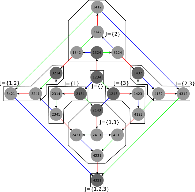
Figure 2. The decomposition of $H_{0}({\mathfrak{S}_{4}})$ into indecomposable right projective modules. This decomposition follows the partition of ${\mathfrak{S}_{4}}$ into left descent classes, each labelled by its descent set $J$. The blue, red, and green lines indicate the action of $\pi_{1},\pi_{2},$ and $\pi_{3}$ respectively. The darker circles indicate idempotent elements of the monoid.

Example 3.24 (Representation theory of $H_{0}(W)$, continued).

The right projective modules of $H_{0}(W)$ are combinatorial, and described by the decomposition of the right order along left descent classes, as illustrated in Figure 2. Namely, let $P_{J}$ be the right projective module of $H_{0}(W)$ corresponding to the idempotent $\pi_{J}$. Its basis $b_{w}$ is indexed by the elements of $w$ having $J$ as left descent set. The action of $\pi_{i}$ coincides with the usual right action, except that $b_{w}.\pi_{i}=0$ if $w.\pi_{i}$ has a strictly larger left descent set than $w$.

Here we reproduce Norton’s construction of $P_{J}$ [Nor79], as it is close to an explicit description of the isomorphism in the proof of Theorem 3.23. First, notice that the elements $\{\pi_{i}^{-}=(1-\pi_{i})\mid i\in I\}$ are idempotent and satisfy the same Coxeter relations as the $\pi_{i}$. Thus, the set $\{\pi_{i}^{-}\}$ generates a monoid isomorphic to $H_{0}(W)$. For each $J\subseteq I$, let $\pi_{J}^{-}$ be the longest element in the parabolic submonoid associated to $J$ generated by the $\pi_{i}^{-}$ generators, and $\pi_{J}^{+}=\pi_{J}$. For each subset $J\subseteq I$, let $\hat{J}=I\setminus J$. Define $f_{J}=\pi_{\hat{J}}^{-}\pi_{J}^{+}$. Then, $f_{J}\pi_{w}=0$ if $J\subset D_{L}(w)$. It follows that the right module $f_{J}H_{0}(W)$ is isomorphic to $P_{J}$ and its basis $\{f_{J}\pi_{w}\mid D_{L}(w)=J\}$ realizes the combinatorial module of $P_{J}$.

One should notice that the elements $\pi_{\hat{J}}^{-}\pi_{J}^{+}$ are, in general, neither idempotent nor orthogonal. Furthermore, $\pi_{\hat{J}}^{-}\pi_{J}^{+}H_{0}(W)$ is not a submodule of $\pi_{J}H_{0}(W)$ as in the proof of Theorem 3.23.

The description of left projective modules is symmetric.

3.5. Factorizations

It is well-known that the notion of factorization $x=uv$ and of irreducibility play an important role in the study of $\mathcal{J}$-trivial monoids $M$. For example, the irreducible elements of $M$ form the unique minimal generating set of $M$ [Doy84, Doy91]. In this section, we further refine these notions, in order to obtain in the next section a combinatorial description of the quiver of the algebra of $M$.

Let $x$ be an element of $M$, and $e:=\operatorname{lfix}(x)$ and $f:=\operatorname{rfix}(x)$. By Proposition 3.16, if $x=uv$ is a factorization of $x$ such that $eu=e$ (or equivalently $e\leq_{\mathcal{J}}u$), then $u\in\operatorname{lAut}(x)$, that is $ux=x$. Similarly on the right side, $vf=f$ implies that $xv=x$. The existence of such trivial factorizations for any element of $M$, beyond the usual $x=1x=x1$, motivate the introduction of refinements of the usual notion of proper factorizations.

Definition 3.25.

Take $x\in M$, and let $e:=\operatorname{lfix}(x)$ and $f:=\operatorname{rfix}(x)$. A factorization $x=uv$ is

• proper if $u\neq x$ and $v\neq x$;

• non-trivial if $eu\neq e$ and $vf\neq f$ (or equivalently $e\not\leq_{\mathcal{J}}u$ and $f\not\leq_{\mathcal{J}}v$, or $u\notin\operatorname{lAut}(x)$ and $v\notin\operatorname{rAut}(x)$);

• compatible if $u$ and $v$ are non-idempotent and

  $$\operatorname{lfix}(u)=e\,,\quad\operatorname{rfix}(v)=f\,\quad\text{and}\quad\operatorname{rfix}(u)=\operatorname{lfix}(v)\,.$$

Example 3.26.

Among the factorizations of $\pi_{2}\pi_{1}\pi_{3}\pi_{2}$ in $H_{0}({\mathfrak{S}_{4}})$, the following are non-proper and trivial:

$$(\operatorname{id},\pi_{2}\pi_{1}\pi_{3}\pi_{2})\quad(\pi_{2},\pi_{2}\pi_{1}\pi_{3}\pi_{2})\quad(\pi_{2}\pi_{1}\pi_{3}\pi_{2},\operatorname{id})\quad(\pi_{2}\pi_{1}\pi_{3}\pi_{2},\pi_{2})\,.$$

The two following factorizations are proper and trivial:

$$(\pi_{2},\pi_{1}\pi_{3}\pi_{2})\quad(\pi_{2}\pi_{1}\pi_{3},\pi_{2})\,.$$

Here are the non-trivial and incompatible factorizations:

$$\begin{array}[]{ccc}(\pi_{2}\pi_{1},\pi_{3}\pi_{2})&(\pi_{2}\pi_{3},\pi_{1}\pi_{2})&(\pi_{2}\pi_{1},\pi_{1}\pi_{3}\pi_{2})\\ (\pi_{2}\pi_{3},\pi_{1}\pi_{3}\pi_{2})&(\pi_{2}\pi_{1}\pi_{3},\pi_{1}\pi_{2})&(\pi_{2}\pi_{1}\pi_{3},\pi_{3}\pi_{2})\,.\end{array}$$

The only non-trivial and compatible factorization is:

$$(\pi_{2}\pi_{1}\pi_{3},\pi_{1}\pi_{3}\pi_{2})\,.$$

Lemma 3.27.

Any non-trivial factorization is also proper.

Proof.

Indeed by contraposition, if $x=xv$ then $v\in\operatorname{rAut}(x)$ and therefore $\operatorname{rfix}(x)\leq_{\mathcal{J}}v$. The case $x=vx$ can be proved similarly. ∎

Lemma 3.28.

If $x$ is an idempotent, $x$ admits only trivial factorizations.

Proof.

Indeed if $x$ is idempotent then $x=\operatorname{rfix}(x)=\operatorname{lfix}(x)$. Then from $x=uv$, one obtains that $x=xuv$. Therefore $x\leq_{\mathcal{J}}xu\leq_{\mathcal{J}}x$ and therefore $x=xu$. ∎

Lemma 3.29.

Any compatible factorization is non-trivial.

Proof.

Let $x=uv$ be a compatible factorization. Then $\operatorname{lfix}(u)=e$ implies that $eu=u$. Since $u$ is not idempotent it cannot be equal to $e$ so that $eu\neq e$. The same holds on the other side. ∎

We order the factorizations of $x$ by the product $\mathcal{J}$-order: Suppose that $x=uv=u^{\prime}v^{\prime}$. Then we write $(u,v)\leq_{\mathcal{J}}(u^{\prime},v^{\prime})$ if and only if $u\leq_{\mathcal{J}}u^{\prime}$ and $v\leq_{\mathcal{J}}v^{\prime}$.

Lemma 3.30.

If $x=uv$ is a non-trivial factorization which is minimal for the product $\mathcal{J}$-order, then it is compatible.

Proof.

Let $x=uv$ be a minimal non-trivial factorization. Then $(eu,vf)$ with $e=\operatorname{lfix}(x)$ and $f=\operatorname{rfix}(x)$ is a factorization of $x$ which is also clearly non-trivial. By minimality we must have that $u=eu$ and $v=vf$. On the other hand, $\operatorname{lfix}(u)x=\operatorname{lfix}(u)uv=uv=x$, so that $e=\operatorname{lfix}(x)\leq_{\mathcal{J}}\operatorname{lfix}(u)$ and therefore $e=\operatorname{lfix}(u)$. This in turn implies that $u$ is non-idempotent since it is different from its left fix. The same holds on the right side.

It remains to show that $\operatorname{rfix}(u)=\operatorname{lfix}(v)$. If $g$ is an idempotent such that $ug=u$, then $x=u(gv)$ is a non-trivial factorization, because $gvf\leq_{\mathcal{J}}vf<_{\mathcal{J}}f$ so that $gvf\neq f$. Therefore by minimality, $gv=v$. By symmetry $ug=u$ is equivalent to $gv=v$. ∎

Putting together these two last lemmas we obtain:

Proposition 3.31.

Take $x\in M$. Then the following are equivalent:

1. $x$ admits a non-trivial factorization;

2. $x$ admits a compatible factorization.

Definition 3.32.

An element is called irreducible if it admits no proper factorization. The set of all irreducible elements of a monoid $M$ is denoted by $\operatorname{Irred}(M)$.

An element is called c-irreducible if it admits no non-trivial factorization. The set of all c-irreducible elements of a monoid $M$ is denoted by $\operatorname{c-Irred}(M)$.

We also denote by $\operatorname{Q}(M)$ the set of c-irreducible non-idempotent elements.

Remark 3.33.

By Lemma 3.27, $\operatorname{Irred}(M)\subseteq\operatorname{c-Irred}(M)$. In particular $\operatorname{c-Irred}(M)$ generates $M$.

3.6. The Ext-quiver

The goal of this section is to give a combinatorial description of the quiver of the algebra of a $\mathcal{J}$-trivial monoid. We start by recalling some well-known facts about algebras and quivers.

Recall that a quiver $Q$ is a directed graph where loops and multiple arrows between two vertices are allowed. The path algebra $\mathbb{K}Q$ of $Q$ is defined as follows. A path in $Q$ is a sequence of arrows $a_{n}a_{n-1}\cdots a_{3}a_{2}a_{1}$ such that the head of $a_{i+1}$ is equal to the tail of $a_{i}$. The product of the path algebra is defined by concatenating paths if tail and head matches and by zero otherwise. Let $F$ denote the ideal in $\mathbb{K}Q$ generated by the arrows of $Q$. An ideal $I\subseteq\mathbb{K}Q$ is said to be admissible if there exists an integer $m\geq 2$ such that $F^{m}\subseteq I\subseteq F^{2}$. An algebra is called split basic if and only if all the simple $A$-modules are one-dimensional. The relevance of quivers comes from the following theorem:

Theorem 3.34 (See e.g. [ARO97]).

For any finite-dimensional split basic algebra $A$, there is a unique quiver $Q$ such that $A$ is isomorphic to $\mathbb{K}Q/I$ for some admissible ideal $I$.

In other words, the quiver $Q$ can be seen as a first order approximation of the algebra $A$. Note however that the ideal $I$ is not necessarily unique.

The quiver of a split basic $\mathbb{K}$-algebra $A$ can be computed as follows: Let $\{f_{i}\mid i\in E\}$ be a complete system of primitive orthogonal idempotents. There is one vertex $v_{i}$ in $Q$ for each $i\in E$. If $i,j\in E$, then the number of arrows in $Q$ from $v_{i}$ to $v_{j}$ is $\dim f_{i}\big{(}\operatorname{rad}A/\mathord{\operatorname{rad}^{2}A}\big{)}f_{j}$. This construction does not depend on the chosen system of idempotents.

Theorem 3.35.

Let $M$ be a $\mathcal{J}$-trivial monoid. The quiver of the algebra of $M$ is the following:

• There is one vertex $v_{e}$ for each idempotent $e\in E(M)$.

• There is an arrow from $v_{\operatorname{lfix}(x)}$ to $v_{\operatorname{rfix}(x)}$ for every c-irreducible element $x\in\operatorname{Q}(M)$.

This theorem follows from Corollary 3.41 below.

Lemma 3.36.

Let $x\in\operatorname{Q}(M)$ and set $e=\operatorname{lfix}(x)$ and $f=\operatorname{rfix}(x)$. Recall that, by definition, whenever $x=uv$, then either $eu=e$ or $vf=f$. Then,

(3.29) $$[x,e[_{\mathcal{R}}=\{u\in M\mid eu=u\neq e\text{ and }uf=x\}.$$

Proof.

Obviously, $\{u\in M\mid eu=u\neq e\text{ and }uf=x\}\subseteq[x,e[_{\mathcal{R}}$. Now take $u\in[x,e[_{\mathcal{R}}$. Then, $u=ea$ for some $a\in M$ and hence $eu=eea=ea=u\neq e$. Furthermore, we can choose $v$ such that $x=uv$ with $vf=v$. Since $x$ admits no non-trivial factorization, we must have $v=f$. ∎

Proposition 3.37.

Take $x\in\operatorname{Q}(M)$ and let $e:=\operatorname{lfix}(x)$ and $f:=\operatorname{rfix}(x)$. Then, there exists a combinatorial module $M_{x}$ with basis $\epsilon=\epsilon_{x},\xi=\xi_{x}$ and action given by

(3.30) $$\epsilon\cdot m :=\begin{cases}\epsilon&\text{if $m\in[e,1]_{\mathcal{R}}$}\\ \xi&\text{if $m\in[x,1]_{\mathcal{R}}\setminus[e,1]_{\mathcal{R}}$}\\ 0&\text{otherwise,}\end{cases}\qquad\text{and}$$

(3.31) $$\xi\cdot m :=\begin{cases}\xi&\text{if $m\in[f,1]_{\mathcal{R}}$}\\ 0&\text{otherwise.}\end{cases}$$

This module of dimension $2$ is indecomposable, with composition factors given by $[e]+[f]$.

Proof.

We give a concrete realization of $M_{x}$. Let $I_{x}:=eM\setminus[x,e]_{\mathcal{R}}$. This is a right ideal, and we endow the interval $[x,e]_{\mathcal{R}}$ with the quotient structure of $eM/I_{x}$. The second step is to further quotient this module by identifying all elements in $[x,e[_{\mathcal{R}}$. Namely, define

(3.32) $$\begin{split}\Theta:[x,e]_{\mathcal{R}}&\rightarrow M_{x}\\ e&\mapsto\epsilon\\ u&\mapsto\xi\quad\text{for $u\in[x,e[_{\mathcal{R}}.$}\end{split}$$

It remains to prove that this map is compatible with the right action of $M$. This boils down to checking that, for $u\in[x,e[_{\mathcal{R}}$ and $y\in M$:

(3.33) $$uy\in[x,e[_{\mathcal{R}}\quad\Longleftrightarrow\quad y\in[f,1]_{\mathcal{R}}\;.$$

Recall that, by Lemma 3.36, $uf=x$. Hence, for $y\in[f,1]_{\mathcal{R}}$, $uy\geq_{\mathcal{R}}uf=x$. Also, since $u\in[x,e[_{\mathcal{R}}$ we have that $uy<_{\mathcal{R}}e$. Now take $y$ such that $uy\in[x,e[_{\mathcal{R}}$, and let $v=yf$. Then $uv=uyf=x$, while $v=vf$. Therefore, since $x$ is c-irreducible, $v=f$. ∎

Corollary 3.38.

The family $(x-x^{\omega})_{x\in\operatorname{Q}(M)}$ is free modulo $\operatorname{rad}^{2}\mathbb{K}M$.

Proof.

We use a triangularity argument: If some $y\in\mathbb{K}M$ lies in $\operatorname{rad}^{2}\mathbb{K}M$ it must act by zero on all modules without square radical. In particular it must act by zero on all $2$-dimensional modules. Suppose that

(3.34) $$\sum_{x\in\operatorname{Q}(M)}c_{x}(x-x^{\omega})$$

with $c_{x}\in\mathbb{K}$ acts by zero on all the previously constructed modules $M_{x}$. Suppose that some $c_{x}$ is nonzero and choose such an $x_{0}$ maximal in $\mathcal{J}$-order. Consider the module $M:=M_{x_{0}}$. Since $x_{0}\in Q(M)$, $x_{0}$ is not idempotent so that $x_{0}^{\omega}\leq_{\mathcal{J}}x_{0}<_{\mathcal{J}}\operatorname{rfix}(x_{0})$. As a consequence

(3.35) $$\epsilon_{x_{0}}\cdot x_{0}=\xi_{x_{0}}\qquad\text{and}\qquad\epsilon_{x_{0}}\cdot x_{0}^{\omega}=0\,.$$

Moreover, if $x$ is not bigger than $x_{0}$ in $\mathcal{J}$-order, then $x$ is also not bigger than $x_{0}$ in $\mathcal{R}$-order, so that $\epsilon_{x_{0}}\cdot x=0$. Therefore

(3.36) $$\epsilon_{x_{0}}\cdot\left(\sum_{x\in\operatorname{Q}(M)}c_{x}(x-x^{\omega})\right)=c_{x_{0}}\xi_{x_{0}}$$

which must vanish in contradiction with the assumption. ∎

We now show that the square radical $\operatorname{rad}^{2}\mathbb{K}M$ is at least as large as the number of factorizable elements:

Proposition 3.39.

Suppose that $x=uv$ is a non-trivial factorization of $x$. Then

(3.37) $$(u-u^{\omega})(v-v^{\omega})=x+\sum_{y<_{\mathcal{J}}x}c_{y}y$$

for some scalars $c_{y}\in\mathbb{K}$.

Proof.

We need to show that $u^{\omega}v$ and $uv^{\omega}$ are both different from $x$. Suppose that $u^{\omega}v=x$. Then $u^{\omega}x=x$ so that $\operatorname{lfix}(x)\leq_{\mathcal{J}}u^{\omega}$. Since $u\operatorname{lfix}(x)\in\operatorname{lAut}(x)$, we have $\operatorname{lfix}(x)\leq_{\mathcal{J}}u\operatorname{lfix}(x)\leq_{\mathcal{J}}\operatorname{lfix}(x)$. Thus $u\operatorname{lfix}(x)=\operatorname{lfix}(x)$ contradicting the non-triviality of the factorization $uv$. The same reasoning shows that $uv^{\omega}<_{\mathcal{J}}x$. ∎

Corollary 3.40.

The family $(x-x^{\omega})_{x\in\operatorname{Q}(M)}$ is a basis of $\operatorname{rad}\mathbb{K}M/\operatorname{rad}^{2}\mathbb{K}M$.

Proof.

By Corollary 3.38 we know that $\operatorname{rad}\mathbb{K}M/\operatorname{rad}^{2}\mathbb{K}M$ is at least of dimension $\operatorname{Card}(\operatorname{Q}(M))$. We just showed that $\operatorname{rad}^{2}\mathbb{K}M$ is at least of dimension $\operatorname{Card}(M)-\operatorname{Card}(E(M))-\operatorname{Card}(\operatorname{Q}(M))$. Therefore all those inequalities must be equalities. ∎

We conclude by an explicit description of the arrows of the quiver as elements of the monoid algebra.

Corollary 3.41.

For all idempotents $i,j\in E(M)$, the family $(f_{i}(x-x^{\omega})f_{j})$ where $x$ runs along the set of non-idempotent c-irreducible elements such that $\operatorname{lfix}(x)=i$ and $\operatorname{rfix}(x)=j$ is a basis for $f_{i}\operatorname{rad}\mathbb{K}Mf_{j}$ modulo $\operatorname{rad}^{2}\mathbb{K}M$.

Proof.

By Corollary 3.19, one has $(f_{i}xf_{j})=x+\sum_{y<_{\mathcal{J}}x}c_{y}y$. Since $x^{\omega}<_{\mathcal{J}}x$, such a triangularity must also hold for $(f_{i}(x-x^{\omega})f_{j})$. ∎

Remark 3.42.

By Remark 3.33 a $\mathcal{J}$-trivial monoid $M$ is generated by (the labels of) the vertices and the arrows of its quiver.

Lemma 3.43.

If $x$ is in the quiver, then it is of the form $x=epf$ with $p$ irreducible, $e=\operatorname{lfix}(x)$, and $f=\operatorname{rfix}(x)$. Furthermore, if $p$ is idempotent, then $x=ef$.

Proof.

Since $x=ex=xf$, one can always write $x$ as $x=eyf$. Assume that $y$ is not irreducible, and write $y=uv$ with $u,v<_{\mathcal{J}}y$. Then, since $x$ is in the quiver, one has either $eu=e$ or $vf=f$, and therefore $x=euf$ or $x=evf$. Repeating the process inductively eventually leads to $x=epf$ with $p$ irreducible.

Assume further that $p$ is an idempotent. Then, $x=(ep)(pf)$ and therefore $ep=e$ or $pf=f$. In both cases, $x=ef$. ∎

Corollary 3.44.

In a $\mathcal{J}$-trivial monoid generated by idempotents, the quiver is given by a subset of all products $ef$ with $e$ and $f$ idempotents such that $e$ and $f$ are respectively the left and right symbols of $ef$.

3.7. Examples of Cartan matrices and quivers

We now use the results of the previous sections to describe the Cartan matrix and quiver of several monoids. Along the way, we discuss briefly some attempts at describing the radical filtration, and illustrate how certain properties of the monoids (quotients, (anti)automorphisms, …) can sometimes be exploited.

3.7.1. Representation theory of $H_{0}(W)$ (continued)

We start by recovering the description of the quiver of the $0$-Hecke algebra of Duchamp-Hivert-Thibon [DHT02] in type $A$ and of Fayers [Fay05] in general type. We further refine it by providing a natural indexing of the arrows of the quiver by certain elements of $H_{0}(W)$.

Proposition 3.45.

The quiver elements $x\in\operatorname{Q}(M)$ are exactly the products $x=\pi_{J}\pi_{K}$ where $J$ and $K$ are two incomparable subsets of $I$ such that, for any $j\in J\setminus K$ and $k\in K\setminus J$, the generators $\pi_{j}$ and $\pi_{k}$ do not commute.

Proof.

Recall that the idempotents of $H_{0}(W)$ are exactly the $\pi_{J}$ for all subsets $J$ and that by Corollary 3.44, the c-irreducible elements are among the products $\pi_{J}\pi_{K}$.

First of all if $J\subseteq K$ then $\pi_{J}\pi_{K}=\pi_{K}\pi_{J}=\pi_{K}$ so that, for $\pi_{J}\pi_{K}$ to be c-irreducible, $J$ and $K$ have to be incomparable. Now suppose that there exists some $j\in J\setminus K$ and $k\in K\setminus J$ such that $\pi_{j}\pi_{k}=\pi_{k}\pi_{j}$. Then

(3.38) $$\pi_{J}\pi_{K}=\pi_{J}\pi_{j}\pi_{k}\pi_{K}=\pi_{J}\pi_{k}\pi_{j}\pi_{K}\,.$$

But since $k\notin J$, one has $\pi_{J}\pi_{k}\neq\pi_{J}$. Similarly, $\pi_{j}\pi_{K}\neq\pi_{K}$. This implies that $(\pi_{J}\pi_{k},\pi_{j}\pi_{K})$ is a non-trivial factorization of $\pi_{J}\pi_{K}$.

Conversely, suppose that there exists a non-trivial factorization $\pi_{J}\pi_{K}=uv$. Since $\pi_{J}u\neq\pi_{J}$, there must exist some $k\in K\backslash J$ such that $u\leq_{\mathcal{J}}\pi_{k}$ (or equivalently $\pi_{k}$ appears in some and therefore any reduced word for $u$). Similarly, one can find some $j\in J\backslash K$ such that $v\leq_{\mathcal{J}}\pi_{j}$. Then, for $<_{\mathcal{B}}$ as defined in (2.1), that is reversed Bruhat order, we have

$$\pi_{J}\pi_{K}=\pi_{J}uv\pi_{K}\leq_{\mathcal{B}}\pi_{J}\pi_{k}\pi_{j}\pi_{K}\leq_{\mathcal{B}}\pi_{J}\pi_{K}\,,$$

and therefore $\pi_{J}\pi_{k}\pi_{j}\pi_{K}=\pi_{J}\pi_{K}$. Hence the left hand side of this equation can be rewritten to its right hand side using a sequence of applications of the relations of $H_{0}(W)$. Notice that using $\pi_{i}^{2}=\pi_{i}$ or any non trivial braid relation preserves the condition that there exists some $\pi_{k}$ to the left of some $\pi_{j}$. Hence rewriting $\pi_{J}\pi_{k}\pi_{j}\pi_{K}$ into $\pi_{J}\pi_{K}$ requires using the commutation relation $\pi_{k}\pi_{j}=\pi_{j}\pi_{k}$ at some point, as desired. ∎

3.7.2. About the radical filtration

Proposition 3.45 suggests to search for a natural indexing by elements of the monoid not only of the quiver, but of the full Loewy filtration.

Problem 3.46.

Find some statistic $r(m)$ for $m\in M$ such that, for any two idempotents $i,j$ and any integer $k$,

(3.39) $$\dim f_{i}\big{(}\operatorname{rad}^{k}A/\operatorname{rad}^{k+1}A\big{)}f_{j}=\\ \operatorname{Card}\{m\in M\mid r(m)=k,\ \operatorname{lfix}(m)=i,\ \operatorname{rfix}(m)=j\}\,.$$

$$\begin{array}[]{|c|c|}\hline\cr Type&\text{Generating series}\\ \hline\cr A_{1}&2\\ A_{2}&2q+4\\ A_{3}&6q^{2}+10q+8\\ A_{4}&10q^{4}+24q^{3}+38q^{2}+32q+16\\ A_{5}&14q^{7}+48q^{6}+72q^{5}+144q^{4}+172q^{3}+150q^{2}+88q+32\\ \hline\cr B_{2}&2q^{2}+2q+4\\ B_{3}&6q^{4}+10q^{3}+14q^{2}+10q+8\\ B_{4}&12q^{8}+24q^{7}+46q^{6}+60q^{5}+76q^{4}+64q^{3}+54q^{2}+32q+16\\ \hline\cr D_{2}&4\\ D_{3}&6q^{2}+10q+8\\ D_{4}&6q^{6}+12q^{5}+20q^{4}+38q^{3}+62q^{2}+38q+16\\ \hline\cr H_{3}&6q^{8}+10q^{7}+14q^{6}+18q^{5}+22q^{4}+18q^{3}+14q^{2}+10q+8\\ \hline\cr I_{5}&2q^{3}+2q^{2}+2q+4\\ I_{6}&2q^{4}+2q^{3}+2q^{2}+2q+4\\ I_{n}&2q^{n-2}+\dots+2q^{2}+2q+4\\ \hline\cr\end{array}$$

Table 1. The generating series $\sum_{k}\dim\big{(}\operatorname{rad}^{k}A/\operatorname{rad}^{k+1}A\big{)}\ q^{k}$ for the $0$-Hecke algebras $A=\mathbb{K}H_{0}(W)$ of the small Coxeter groups.

Such a statistic is not known for $H_{0}(W)$, even in type $A$. Its expected generating series for small Coxeter group is shown in Table 1. Note that all the coefficients appearing there are even. This is a general fact:

Proposition 3.47.

Let $W$ be a Coxeter group and $H_{0}(W)$ its $0$-Hecke monoid. Then, for any $k$, the dimension $d^{k}:=\dim\operatorname{rad}^{k}\mathbb{K}H_{0}(W)$ is an even number.

Proof.

This is a consequence of the involutive algebra automorphism $\theta\ :\ \pi_{i}\mapsto 1-\pi_{i}$. This automorphism exchanges the eigenvalues 0 and 1 for the idempotent $\pi_{i}$. Therefore it exchanges the projective module $P_{J}$ associated to the descent set $J$ (see Example 3.9 for the definition of $P_{J}$) with the projective module $P_{\overline{J}}$ associated to the complementary descent set $\overline{J}=I\setminus J$. As a consequence it must exchange $\operatorname{rad}^{k}P_{J}$ and $\operatorname{rad}^{k}P_{\overline{J}}$ which therefore have the same dimensions. Since there is no self-complementary descent set, $d^{k}=\sum_{J\subset I}\operatorname{rad}^{k}P_{J}$ must be even. ∎

Also, as suggested by Table 1, Problem 3.46 admits a simple solution for $H_{0}(I_{n})$.

Proposition 3.48.

Let $W$ be the $n$-th dihedral group (type $I_{n}$) and $\mathbb{K}H_{0}(W)$ its $0$-Hecke algebra. Define $a_{k}=\pi_{1}\pi_{2}\pi_{1}\pi_{2}\cdots$ and $b_{k}=\pi_{2}\pi_{1}\pi_{2}\pi_{1}\cdots$ where both words are of length $k$. Recall that the longest element of $H_{0}(W)$ is $\omega=a_{n}=b_{n}$. Then, for all $k>0$, the set

(3.40) $$R_{k}:=\{a_{i}-\omega,\ b_{i}-\omega\mid k<i<n\}$$

is a basis for $\operatorname{rad}^{k}\mathbb{K}H_{0}(W)$. In particular, defining the statistic $r(w):=\ell(w)-1$, one obtains that the family

$$\{a_{k+1}-\omega,b_{k+1}-\omega\}$$

for $0<k<n-1$ is a basis of $\operatorname{rad}^{k}\mathbb{K}H_{0}(W)/\operatorname{rad}^{k+1}\mathbb{K}H_{0}(W)$.

Note that if $k<n-1$ then $\omega$ belongs to $\operatorname{rad}^{k+1}\mathbb{K}H_{0}(W)$. One can therefore take $\{a_{k+1},b_{k+1}\}$ as a basis.

Proof.

The case $k=1$ follows from Proposition 3.3, and by Proposition 3.40 the quiver is given by $a_{2}-\omega$ and $b_{2}-\omega$. The other cases are then proved by induction, using the following relations:

$$(a_{2}-\omega)(a_{j}-\omega) =a_{j+2}-\omega \qquad(a_{2}-\omega)(b_{j}-\omega) =a_{j+1}-\omega$$

$$(b_{2}-\omega)(b_{j}-\omega) =b_{j+2}-\omega (b_{2}-\omega)(a_{j}-\omega) =b_{j+1}-\omega.\qed$$

A natural approach to try to define such a statistic $r(m)$ is to use iterated compatible factorizations. For example, one can define a new product $\bullet$, called the compatible product on $M\cup\{0\}$, as follows:

$$x\bullet y=\begin{cases}xy&\text{if $\operatorname{lfix}(x)=\operatorname{lfix}(xy)$ and $\operatorname{rfix}(y)=\operatorname{rfix}(xy)$ and $\operatorname{rfix}(x)=\operatorname{lfix}(y)$,}\\ 0&\text{otherwise.}\end{cases}$$

However this product is usually not associative. Take for example $x=\pi_{14352}$, $y=\pi_{31254}$ and $z=\pi_{25314}$ in $H_{0}({\mathfrak{S}_{5}})$. Then, $xy=\pi_{41352}$, $yz=\pi_{35214}$ and $xyz=\pi_{45312}$. The following table shows the left and right descents of those elements:

$$\begin{array}[]{r|c|c}&\text{left}&\text{right}\\ \hline\cr x=\pi_{14352}&\{2,3\}&\{2,4\}\\ y=\pi_{31254}&\{2,4\}&\{1,4\}\\ z=\pi_{25314}&\{1,4\}&\{2,3\}\\ xy=\pi_{41352}&\{2,3\}&\{1,4\}\\ yz=\pi_{35214}&\{1,2,4\}&\{2,3\}\\ xyz=\pi_{45312}&\{2,3\}&\{2,3\}\\ \end{array}$$

Consequently $(x\bullet y)\bullet z=(xy)\bullet z=xyz$ whereas $y\bullet z=0$ and therefore $x\bullet(y\bullet z)=0$.

Due to the lack of associativity there is no immediate definition for $r(m)$ as the “length of the longest compatible factorization”, and our various attempts to define this concept all failed for the $0$-Hecke algebra in type $D_{4}$.

3.7.3. Nondecreasing parking functions

We present, without proof, how the description of the Cartan matrix of ${\operatorname{NDPF}}_{n}$ in [HT06, HT09] fits within the theory, and derive its quiver from that of $H_{0}({\mathfrak{S}_{n}})$.

Proposition 3.49.

The idempotents of ${\operatorname{NDPF}}_{n}$ are characterized by their image sets, and there is one such idempotent for each subset of $\{1,\dots,n\}$ containing $1$. For $f$ an element of ${\operatorname{NDPF}}_{n}$, $\operatorname{rfix}(f)$ is given by the image set of $f$, whereas $\operatorname{lfix}(f)$ is given by the set of all lowest point in each fiber of $f$; furthermore, $f$ is completely characterized by $\operatorname{lfix}(f)$ and $\operatorname{rfix}(f)$.

The Cartan matrix is $0,1$, with $c_{I,J}=1$ if $I=\{i_{1}<\cdots<i_{k}\}$ and $J=\{j_{1}<\cdots<j_{k}\}$ are two subsets of the same cardinality $k$ with $i_{l}\leq j_{l}$ for all $l$.

Proposition 3.50.

Let $M$ be a $\mathcal{J}$-trivial monoid generated by idempotents. Suppose that $N$ is a quotient of $M$ such that $E(N)=E(M)$. Then, the quiver of $N$ is a subgraph of the quiver of $M$.

Note that the hypothesis implies that $M$ and $N$ have the same generating set.

Proof.

It is easy to see that $\operatorname{lfix}$ and $\operatorname{rfix}$ are the same in $M$ and $N$. Moreover, any compatible factorization in $M$ is still a compatible factorization in $N$. ∎

As a consequence one recovers the quiver of ${\operatorname{NDPF}}_{n}$:

Proposition 3.51.

The quiver elements of ${\operatorname{NDPF}}_{n}$ are the products $\pi_{J\cup\{i\}}\pi_{J\cup\{i+1\}}$ where $J\subset\{1,\dots,n-1\}$ and $i,i+1\notin J$.

Proof.

Recall that ${\operatorname{NDPF}}_{n}$ is the quotient of $H_{0}({\mathfrak{S}_{n}})$ by the relation $\pi_{i}\pi_{i+1}\pi_{i}=\pi_{i+1}\pi_{i}$, via the quotient map $\pi_{i}\mapsto\pi_{i}$. For $J$ a subset of $\{1,\dots,n-1\}$, define accordingly $\pi_{J}$ in ${\operatorname{NDPF}}_{n}$ as the image of $\pi_{J}$ in $H_{0}({\mathfrak{S}_{n}})$. Specializing Proposition 3.45 to type $A_{n-1}$, one obtains that there are four types of quiver elements:

• $\pi_{J\cup\{i\}}\pi_{J\cup\{i+1\}}$ where $J\subset\{1,\dots,n-1\}$ and $i,i+1\notin J$,

• $\pi_{J\cup\{i+1\}}\pi_{J\cup\{i\}}$ where $J\subset\{1,\dots,n-1\}$ and $i,i+1\notin J$,

• $\pi_{K\cup\{i,i+2\}}\pi_{K\cup\{i+1\}}$ where $K\subset\{1,\dots,n-1\}$ and $i,i+1,i+2\notin K$,

• $\pi_{K\cup\{i+1\}}\pi_{K\cup\{i,i+2\}}$ where $K\subset\{1,\dots,n-1\}$ and $i,i+1,i+2\notin K$.

One can easily check that the three following factorizations are non-trivial:

• $\pi_{J\cup\{i+1\}}\pi_{J\cup\{i\}}=(\pi_{J\cup\{i+1\}}\pi_{i},\ \pi_{i+1}\pi_{J\cup\{i\}})$,

• $\pi_{K\cup\{i,i+2\}}\pi_{K\cup\{i+1\}}=(\pi_{K\cup\{i,i+2\}}\pi_{i+1},\ \pi_{i+2}\pi_{K\cup\{i+1\}})$,

• $\pi_{K\cup\{i+1\}}\pi_{K\cup\{i,i+2\}}=(\pi_{K\cup\{i+1\}}\pi_{i},\ \pi_{i+1}\pi_{K\cup\{i,i+2\}})$.

Conversely, any non-trivial factorization of $\pi_{J\cup\{i\}}\pi_{J\cup\{i+1\}}$ in ${\operatorname{NDPF}}_{n}$ would have been non-trivial in the Hecke monoid. ∎

3.7.4. The incidence algebra of a poset

We show now that we can recover the well-known representation theory of the incidence algebra of a partially ordered set.

Let $(P,\leq)$ be a partially ordered set. Recall that the incidence algebra of $P$ is the algebra $\mathbb{K}P$ whose basis is the set of pairs $(x,y)$ of comparable elements $x\leq y$ with the product rule

(3.41) $$(x,y)(z,t)=\begin{cases}(x,t)&\text{if $y=z$,}\\ 0&\text{otherwise.}\end{cases}$$

The incidence algebra is very close to the algebra of a monoid except that $0$ and $1$ are missing. We therefore build a monoid by adding $0$ and $1$ artificially and removing them at the end:

Definition 3.52.

Let $(P,\leq)$ be a partially ordered set. Let $\operatorname{Zero}$ and $\operatorname{One}$ be two elements not in $P$. The incidence monoid of $P$ is the monoid $M(P)$, whose underlying set is

$$M(P):=\{(x,y)\in P\mid x\leq y\}\cup\{\operatorname{Zero},\operatorname{One}\}\,,$$

with the product rule given by Equation 3.41 plus $\operatorname{One}$ being neutral and $\operatorname{Zero}$ absorbing.

Proposition 3.53.

Define an order $\preceq$ on $M(P)$ by

(3.42) $$(x,y)\preceq(z,t)\quad\text{if and only if}\quad x\leq z\leq t\leq y\,,$$

and $\operatorname{One}$ and $\operatorname{Zero}$ being the largest and the smallest element, respectively. The monoid $M(P)$ is left-right ordered for $\preceq$ and thus $\mathcal{J}$-trivial.

Proof.

This is trivial by the product rule. ∎

One can now use all the results on $\mathcal{J}$-trivial monoids to obtain the representation theory of $M(P)$. One gets back to $\mathbb{K}P$ thanks to the following result.

Proposition 3.54.

As an algebra, $\mathbb{K}M(P)$ is isomorphic to $\mathbb{K}\operatorname{One}\ \oplus\ \mathbb{K}P\ \oplus\ \mathbb{K}\operatorname{Zero}$.

Proof.

In the monoid algebra $\mathbb{K}M(P)$, the elements $(x,x)$ are orthogonal idempotents. Thus $e:=\sum_{x\in P}(x,x)$ is itself an idempotent and it is easily seen that $\mathbb{K}P$ is isomorphic to $e(\mathbb{K}M(P))e$. ∎

One can then easily deduce the representation theory of $\mathbb{K}P$:

Proposition 3.55.

Let $(P,\leq)$ be a partially ordered set and $\mathbb{K}P$ its incidence algebra. Then the Cartan matrix $C=(c_{x,y})_{x,y\in P}$ of $\mathbb{K}P$ is indexed by $P$ and given by

$$c_{x,y}=\begin{cases}1&\text{if $x\leq y\,,$}\\ 0&\text{otherwise.}\end{cases}$$

The arrows of the quiver are $x\to y$ whenever $(x,y)$ is a cover in $P$, that is, $x\leq y$ and there is no $z$ such that $x\leq z\leq y$.

Proof.

Clearly $\operatorname{lfix}(x,y)=(x,x)$ and $\operatorname{rfix}(x,y)=(y,y)$. Moreover, the compatible factorizations of $(x,y)$ are exactly $(x,z)(z,y)$ with $x<z<y$. ∎

3.7.5. Unitriangular Boolean matrices

Next we consider the monoid of unitriangular Boolean matrices $\mathcal{U}_{n}$.

Remark 3.56.

The idempotents of $\mathcal{U}_{n}$ are in bijection with the posets admitting $1,\dots,n$ as linear extension (sequence A006455 in [Se03]).

Let $m\in\mathcal{U}_{n}$ and $g$ be the corresponding digraph. Then $m^{\omega}$ is the transitive closure of $g$, and $\operatorname{lfix}(g)$ and $\operatorname{rfix}(g)$ are given respectively by the largest “prefix” and “postfix” of $g$ which are posets: namely, $\operatorname{lfix}(g)$ (resp. $\operatorname{rfix}(g)$) correspond to the subgraph of $g$ containing the edges $i\!\!\rightarrow\!\!j$ (resp. $j\!\!\rightarrow\!\!k$) of $g$ such that $i\!\!\rightarrow\!\!k$ is in $g$ whenever $j\!\!\rightarrow\!\!k$ (resp. $i\!\!\rightarrow\!\!j$) is.

Figure 3 displays the Cartan matrix and quiver of $\mathcal{U}_{4}$; as expected, their nodes are labelled by the 40 subposets of the chain. This figure further suggests that they are acyclic and enjoy a certain symmetry, properties which we now prove in general.

Figure 3. On top, the Cartan matrix (drawn as a graph) and at the bottom the quiver of $\mathcal{U}_{4}$. The edge labels have not been drawn for readability; for the quiver, they can be recovered as the product of two vertices. Those pictures have been produced automatically by Sage, dot2tex, and graphviz, up to a manual reorganization of the connected components using inkscape.

The monoid $\mathcal{U}_{n}$ admits a natural antiautomorphism $\phi$; it maps an upper triangular Boolean matrix to its transpose along the second diagonal or, equivalently, relabels the vertices of the corresponding digraph by $i\mapsto n-i$ and then takes the dual.

Proposition 3.57.

The Cartan matrix of $\mathcal{U}_{n}$, seen as a graph, and its quiver are preserved by the non-trivial antiautomorphism induced by $\phi$.

Proof.

Remark that any antiautomorphism $\phi$ flips $\operatorname{lfix}$ and $\operatorname{rfix}$:

$$\operatorname{lfix}(\phi(x))=\operatorname{rfix}(x)\qquad\text{and}\qquad\operatorname{rfix}(\phi(x))=\operatorname{lfix}(x)\,,$$

and that the definition of $c$-irreducible is symmetric. ∎

Fix an ordering of the pairs $(i,j)$ with $i<j$ such that $(i,j)$ always comes before $(j,k)$ (for example using lexicographic order). Compare two elements of $\mathcal{U}_{n}$ lexicographically by writing them as bit vectors along the chosen enumeration of the pairs $(i,j)$.

Proposition 3.58.

The Cartan matrix of $\mathcal{U}_{n}$ is unitriangular with respect to the chosen order, and therefore its quiver is acyclic.

Proof.

We prove that, if $e=\operatorname{lfix}(g)$ and $f=\operatorname{rfix}(g)$, then $e\leq f$, with equality if and only if $g$ is idempotent.

If $g$ is idempotent, then $e=f=g$, and we are done. Assume now that $g$ is not idempotent, so that $e\neq g$ and $f\neq g$. Take the smallest edge $j\!\!\rightarrow\!\!k$ which is in $g$ but not in $f$. Then, there exists $i<j$ such that $i\!\!\rightarrow\!\!k$ is not in $g$ but $i\!\!\rightarrow\!\!j$ is. Therefore $i\!\!\rightarrow\!\!j$ is not in $e$, whereas by minimality it is in $f$. Hence, $f>e$, as desired. ∎

Looking further at Figure 3 suggests that the quiver is obtained as the transitive reduction of the Cartan matrix; we checked on computer that this property still holds for $n=5$ and $n=6$.

3.7.6. $\mathcal{J}$-trivial monoids built from quivers

We conclude with a collection of examples showing in particular that any quiver can be obtained as quiver of a finite $\mathcal{J}$-trivial monoid.

Example 3.59.

Consider a finite commutative idempotent $\mathcal{J}$-trivial monoid, that is a finite lattice $L$ endowed with its meet operation. Denote accordingly by $0$ and $1$ the bottom and top elements of $L$. Extend $L$ by a new generator $p$, subject to the relations $pep=0$ for all $e$ in $L$, to get a $\mathcal{J}$-trivial monoid $M$ with elements given by $L\uplus\{epf\mid e,f\in L\}$.

Then, the quiver of $M$ is a complete digraph: its vertices are the elements of $L$, and between any two elements $e$ and $f$ of $L$, there is a single edge which is labelled by $epf$.

Example 3.60.

Consider any finite quiver $G=(E,Q)$, that is a digraph, possibly with loops, cycles, or multiple edges, and with distinct labels on all edges. We denote by ${e\!\stackrel{{\scriptstyle l}}{{\rightarrow}}\!\!f}$ an edge in $Q$ from $e$ to $f$ with label $l$.

Define a monoid $M(G)$ on the set $E\uplus Q\uplus\{0,1\}$ by the following product rules:

$$e^{2} \ =\ e e\in E$$ for all ,

$$e\ {e\!\stackrel{{\scriptstyle l}}{{\rightarrow}}\!\!f} \ =\ {e\!\stackrel{{\scriptstyle l}}{{\rightarrow}}\!\!f} {e\!\stackrel{{\scriptstyle l}}{{\rightarrow}}\!\!f}\in Q$$ for all ,

$${e\!\stackrel{{\scriptstyle l}}{{\rightarrow}}\!\!f}\ f \ =\ {e\!\stackrel{{\scriptstyle l}}{{\rightarrow}}\!\!f} {e\!\stackrel{{\scriptstyle l}}{{\rightarrow}}\!\!f}\in Q$$ for all ,

together with the usual product rule for $1$, and all other products being $0$. In other words, this is the quotient of the path monoid $P(G)$ of $G$ (which is $\mathcal{J}$-trivial) obtained by setting $p=0$ for all paths $p$ of length at least two.

Then, $M(G)$ is a $\mathcal{J}$-trivial monoid, and its quiver is $G$ with $0$ and $1$ added as extra isolated vertices. Those extra vertices can be eliminated by considering instead the analogous quotient of the path algebra of $G$ (i.e. setting $0_{M(G)}=0_{\mathbb{K}}$ and $1_{M(G)}=\sum_{g\in E}g$).

Example 3.61.

Choose further a lattice structure $L$ on $E\cup\{0,1\}$. Define a $\mathcal{J}$-trivial monoid $M(G,L)$ on the set $E\uplus Q\uplus\{0,1\}$ by the following product rules:

$$ef \ =\ e\vee_{L}f e,f\in E$$ for all ,

$${e\!\stackrel{{\scriptstyle l}}{{\rightarrow}}\!\!f}\ f^{\prime} \ =\ {e\!\stackrel{{\scriptstyle l}}{{\rightarrow}}\!\!f} {e\!\stackrel{{\scriptstyle l}}{{\rightarrow}}\!\!f}\in Q f^{\prime}\in E f\leq_{L}f^{\prime}$$ for all and with ,

$$e^{\prime}\ {e\!\stackrel{{\scriptstyle l}}{{\rightarrow}}\!\!f} \ =\ {e\!\stackrel{{\scriptstyle l}}{{\rightarrow}}\!\!f} {e\!\stackrel{{\scriptstyle l}}{{\rightarrow}}\!\!f}\in Q e^{\prime}\in E e\leq_{L}e^{\prime}$$ for all and with ,

together with the usual product rule for $1$, and all other products being $0$. Note that the monoid $M(G)$ of the previous example is obtained by taking for $L$ the lattice where the vertices of $G$ form an antichain. Then, the semi-simple quotient of $M(G,L)$ is $L$ and its quiver is $G$ (with $0$ and $1$ added as extra isolated vertices).

Example 3.62.

We now assume that $G=(E,Q)$ is a simple quiver. Namely, there are no loops, and between two distinct vertices $e$ and $f$ there is at most one edge which we denote by $e\,\!\!\rightarrow\!\!f$ for short. Define a monoid structure $M^{\prime}(G)$ on the set $E\uplus Q\uplus\{0,1\}$ by the following product rules:

$$e^{2} \ =\ e e\in E$$ for all ,

$$ef \ =\ e\,\!\!\rightarrow\!\!f e\,\!\!\rightarrow\!\!f\in Q$$ for all ,

$$e\ e\,\!\!\rightarrow\!\!f \ =\ e\,\!\!\rightarrow\!\!f e\,\!\!\rightarrow\!\!f\in Q$$ for all ,

$$e\,\!\!\rightarrow\!\!f\ f \ =\ e\,\!\!\rightarrow\!\!f e\,\!\!\rightarrow\!\!f\in Q$$ for all ,

together with the usual product rule for $1$, and all other products being $0$.

Then, $M^{\prime}(G)$ is a $\mathcal{J}$-trivial monoid generated by the idempotents in $E$ and its quiver is $G$ (with $0$ and $1$ added as extra isolated vertices).

Exercise 3.63.

Let $L$ be a lattice structure on $E\cup\{0,1\}$. Find compatibility conditions between $G$ and $L$ for the existence of a $\mathcal{J}$-trivial monoid generated by idempotents having $L$ as semi-simple quotient and $G$ (with $0$ and $1$ added as extra isolated vertices) as quiver.

3.8. Implementation and complexity

The combinatorial description of the representation theoretical properties of a $\mathcal{J}$-trivial monoid (idempotents, Cartan matrix, quiver) translate straightforwardly into algorithms. Those algorithms have been implemented by the authors, in the open source mathematical system Sage [S⁺09], in order to support their own research. The code is publicly available from the Sage-Combinat patch server [SCc08], and is being integrated into the main Sage library and generalized to larger classes of monoids in collaboration with other Sage-Combinat developers. It is also possible to delegate all the low-level monoid calculations (Cayley graphs, $\mathcal{J}$-order, …) to the blazingly fast $C$ library Semigroupe by Jean-Éric Pin [Pin10b].

We start with a quick overview of the complexity of the algorithms.

Proposition 3.64.

In the statements below, $M$ is a $\mathcal{J}$-trivial monoid of cardinality $n$, constructed from a set of $m\leq n$ generators $s_{1},\dots,s_{m}$ in some ambient monoid. The product in the ambient monoid is assumed to be $O(1)$. All complexity statements are upper bounds, with no claim for optimality. In practice, the number of generators is usually small; however the number of idempotents, which condition the size of the Cartan matrix and of the quiver, can be as large as $2^{m}$.

1. Construction of the left / right Cayley graph: $O(nm)$ (in practice it usually requires little more than $n$ operations in the ambient monoid);

2. Sorting of elements according to $\mathcal{J}$-order: $O(nm)$;

3. Selection of idempotents: $O(n)$;

4. Calculation of all left and right symbols: $O(nm)$;

5. Calculation of the Cartan matrix: $O(nm)$;

6. Calculation of the quiver: $O(n^{2})$.

Proof.

a: See [FP97]

b: This is a topological sort calculation for the two sided Cayley graph which has $n$ nodes and $2nm$ edges.

c: Brute force selection.

For each of the following steps, we propose a simple algorithm satisfying the claimed complexity.

d: Construct, for each element $x$ of the monoid, two bit-vectors $l(x)=(l_{1},\dots,l_{m})$ and $r(x)=(r_{1},\dots,r_{m})$ with $l_{i}=\delta_{s_{i}x,x}$ and $r_{i}=\delta_{xs_{i},x}$. This information is trivial to extract in $O(nm)$ from the left and right Cayley graphs, and could typically be constructed as a side effect of a. Those bit-vectors describe uniquely $\operatorname{lAut}(x)$ and $\operatorname{rAut}(x)$. From that, one can recover all $\operatorname{lfix}(x)$ and $\operatorname{rfix}(x)$ in $O(nm)$: as a precomputation, run through all idempotents $e$ of $M$ to construct a binary prefix tree $T$ which maps $l(e)=r(e)$ to $e$; then, for each $x$ in $M$, use $T$ to recover $\operatorname{lfix}(x)$ and $\operatorname{rfix}(x)$ from the bit vectors $l(x)$ and $r(x)$.

e: Obviously $O(n)$ once all left and right symbols have been calculated; so $O(nm)$ altogether.

f: A crude algorithm is to compute all products $xy$ in the monoid, check whether the factorization is compatible, and if yes cross the result out of the quiver (brute force sieve). This can be improved by running only through the products $xy$ with $\operatorname{rfix}(x)=\operatorname{lfix}(y)$; however this does not change the worst case complexity (consider a monoid with only $2$ idempotents $0$ and $1$, like $\mathbb{N}^{m}$ truncated by any ideal containing all but $n-2$ elements, so that $\operatorname{lfix}(x)=\operatorname{rfix}(x)=1$ for all $x\neq 0$). ∎

We conclude with a sample session illustrating typical calculations, using Sage 4.5.2 together with the Sage-Combinat patches, running on Ubuntu Linux 10.5 on a Macbook Pro 4.1. Note that the interface is subject to minor changes before the final integration into Sage. The authors will gladly provide help in using the software.

We start by constructing the $0$-Hecke monoid of the symmetric group $W={\mathfrak{S}_{4}}$, through its action on $W$:

\small
  sage: W = SymmetricGroup(4)
  sage: S = semigroupe.AutomaticSemigroup(W.simple_projections(), W.one(),
  ...                  by_action = True, category=FiniteJTrivialMonoids())
  sage: S.cardinality()
  24

We check that it is indeed $\mathcal{J}$-trivial, and compute its $8$ idempotents:

\small
  sage: S._test_j_trivial()
  sage: S.idempotents()
  [[], [1], [2], [3], [1, 3], [1, 2, 1], [2, 3, 2], [1, 2, 1, 3, 2, 1]]

Here is its Cartan matrix and its quiver:

\small
    sage: S.cartan_matrix_as_graph().adjacency_matrix(), S.quiver().adjacency_matrix()
    (
    [0 0 0 0 0 0 0 0]  [0 0 0 0 0 0 0 0]
    [0 0 1 0 1 1 0 0]  [0 0 1 0 1 1 0 0]
    [0 1 0 0 1 0 0 0]  [0 1 0 0 0 0 0 0]
    [0 0 0 0 0 0 0 0]  [0 0 0 0 0 0 0 0]
    [0 1 1 0 0 0 0 0]  [0 1 0 0 0 0 0 0]
    [0 1 0 0 0 0 1 1]  [0 1 0 0 0 0 1 1]
    [0 0 0 0 0 1 0 1]  [0 0 0 0 0 1 0 0]
    [0 0 0 0 0 1 1 0], [0 0 0 0 0 1 0 0]
    )

In the following example, we check that, for any of the $318$ posets $P$ on $6$ vertices, the Cartan matrix $m$ of the monoid $\mathcal{OR}(P)$ of order preserving nondecreasing functions on $P$ is unitriangular. To this end, we check that the digraph having $m-1$ as adjacency matrix is acyclic.

\small
sage: from sage.combinat.j_trivial_monoids import *
sage: @parallel
...def check_cartan_matrix(P):
...    return DiGraph(NDPFMonoidPoset(P).cartan_matrix()-1).is_directed_acyclic()
sage: time all(res[1] for res in check_cartan_matrix(list(Posets(6))))
CPU times: user 5.68 s, sys: 2.00 s, total: 7.68 s
Wall time: 255.53 s
True

Note: the calculation was run in parallel on two processors, and the displayed CPU time is just that of the master process, which is not much relevant. The same calculation on a eight processors machine takes about 71 seconds.

We conclude with the calculation of the representation theory of a larger example (the monoid $\mathcal{U}_{n}$ of unitriangular Boolean matrices). The current implementation is far from optimized: in principle, the cost of calculating the Cartan matrix should be of the same order of magnitude as generating the monoid. Yet, this implementation makes it possible to explore routinely, if not instantly, large Cartan matrices or quivers that were completely out of reach using general purpose representation theory software.

\small
  M = semigroupe.UnitriangularBooleanMatrixSemigroup(6)
  Loading Sage library. Current Mercurial branch is: combinat
  sage: time M.cardinality()
  CPU times: user 0.14 s, sys: 0.02 s, total: 0.16 s
  Wall time: 0.16 s
  32768
  sage: time M.cartan_matrix()
  CPU times: user 27.50 s, sys: 0.09 s, total: 27.59 s
  Wall time: 27.77 s
  4824 x 4824 sparse matrix over Integer Ring
  sage: time M.quiver()
  CPU times: user 512.73 s, sys: 2.81 s, total: 515.54 s
  Wall time: 517.55 s
  Digraph on 4824 vertices

Figure 3 displays the results in the case $n=4$.

4. Monoid of order preserving regressive functions on a poset $P$

In this section, we discuss the monoid $\mathcal{OR}(P)$ of order preserving regressive functions on a poset $P$. Recall that this is the monoid of functions $f$ on $P$ such that for any $x\leq y\in P$, $x.f\leq x$ and $x.f\leq y.f$.

In Section 4.1, we discuss constructions for idempotents in $\mathcal{OR}(P)$ in terms of the image sets of the idempotents, as well as methods for obtaining $\operatorname{lfix}(f)$ and $\operatorname{rfix}(f)$ for any given function $f$. In Section 4.2, we show that the Cartan matrix for $\mathcal{OR}(P)$ is upper uni-triangular with respect to the lexicographic order associated to any linear extension of $P$. In Section 4.3, we specialize to $\mathcal{OR}(L)$ where $L$ is a meet semi-lattice, describing a minimal generating set of idempotents. Finally, in Section 4.4, we describe a simple construction for a set of orthogonal idempotents in ${\operatorname{NDPF}}_{N}$, and present a conjectural construction for orthogonal idempotents for $\mathcal{OR}(L)$.

4.1. Combinatorics of idempotents

The goal of this section is to describe the idempotents in $\mathcal{OR}(P)$ using order considerations. We begin by giving the definition of joins, even in the setting when the poset $P$ is not a lattice.

Definition 4.1.

Let $P$ be a finite poset and $S\subseteq P$. Then $z\in P$ is called a join of $S$ if $x\leq z$ holds for any $x\in S$, and $z$ is minimal with that property.

We denote $\operatorname{Joins}(S)$ the set of joins of $S$, and $\operatorname{Joins}(x,y)$ for short if $S=\{x,y\}$. If $\operatorname{Joins}(S)$ (resp. $\operatorname{Joins}(x,y)$) is a singleton (for example because $P$ is a lattice) then we denote $\bigvee S$ (resp. $x\vee y$) the unique join. Finally, we define $\operatorname{Joins}(\emptyset)$ to be the set of minimal elements in $P$.

Lemma 4.2.

Let $P$ be some poset, and $f\in\mathcal{OR}(P)$. If $x$ and $y$ are fixed points of $f$, and $z$ is a join of $x$ and $y$, then $z$ is a fixed point of $f$.

Proof.

Since $x\leq z$ and $y\leq z$, one has $x=x.f\leq z.f$ and $y=y.f\leq z.f$. Since furthermore $z.f\leq z$, by minimality of $z$ the equality $z.f=z$ must hold. ∎

Lemma 4.3.

Let $I$ be a subset of $P$ which contains all the minimal elements of $P$ and is stable under joins. Then, for any $x\in P$, the set $\{y\in I\mid y\leq x\}$ admits a unique maximal element which we denote by $\sup_{I}(x)\in I$. Furthermore, the map $\sup_{I}:x\mapsto\sup_{I}(x)$ is an idempotent in $\mathcal{OR}(P)$.

Proof.

For the first statement, suppose for some $x\not\in I$ there are two maximal elements $y_{1}$ and $y_{2}$ in $\{y\in I\mid y\leq x\}$. Then the join $y_{1}\wedge y_{2}<x$, since otherwise $x$ would be a join of $y_{1}$ and $y_{2}$, and thus $x\in I$ since $I$ is join-closed. But this contradicts the maximality of $y_{1}$ and $y_{2}$, so the first statement holds.

Using that $\sup_{I}(x)\leq x$ and $\sup_{I}(x)\in I$, $e:=\sup_{I}$ is a regressive idempotent by construction. Furthermore, it is is order preserving: for $x\leq z$, $x.e$ and $z.e$ must be comparable or else there would be two maximal elements in $I$ under $z$. Since $z.e$ is maximal under $z$, we have $z.e\geq x.e$. ∎

Reciprocally, all idempotents are of this form:

Lemma 4.4.

Let $P$ be some poset, and $f\in\mathcal{OR}(P)$ be an idempotent. Then the image $\operatorname{im}(f)$ of $f$ satisfies the following:

1. All minimal elements of $P$ are contained in $\operatorname{im}(f)$.

2. Each $x\in\operatorname{im}(f)$ is a fixed point of $f$.

3. The set $\operatorname{im}(f)$ is stable under joins: if $S\subseteq\operatorname{im}(f)$ then $\operatorname{Joins}(S)\subseteq\operatorname{im}(f)$ .

4. For any $x\in P$, the image $x.f$ is the upper bound $\sup_{\operatorname{im}(f)}(x)$.

Proof.

Statement (1) follows from the fact that $x.f\leq x$ so that minimal elements must be fixed points and hence in $\operatorname{im}(f)$.

For any $x=a.f$, if $x$ is not a fixed point then $x.f=(a.f).f\neq a.f$, contradicting the idempotence of $f$. Thus, the second statement holds.

Statement (3) follows directly from the second statement and Lemma 4.2.

If $y\in\operatorname{im}(f)$ and $y\leq x$ then $y=y.f\leq x.f$. Since this holds for every element of $\{y\in\operatorname{im}(f)\mid y\leq x\}$ and $x.f$ is itself in this set, statement (4) holds. ∎

Thus, putting together Lemmas 4.3 and 4.4 one obtains a complete description of the idempotents of $\mathcal{OR}(P)$.

Proposition 4.5.

The idempotents of $\mathcal{OR}(P)$ are given by the maps $\sup_{I}$, where $I$ ranges through the subsets of $P$ which contain the minimal elements and are stable under joins.

For $f\in\mathcal{OR}(P)$ and $y\in P$, let $f^{-1}(y)$ be the fiber of $y$ under $f$, that is, the set of all $x\in P$ such that $x.f=y$.

Definition 4.6.

Given $S$ a subset of a finite poset $P$, set $C_{0}(S)=S$ and $C_{i+1}(S)=C_{i}(S)\cup\{x\in P\mid x\text{ is a join of some elements in }C_{i}(S)\}$. Since $P$ is finite, there exists some $N$ such that $C_{N}(S)=C_{N+1}(S)$. The join closure is defined as this stable set, and denoted $C(S)$. A set is join-closed if $C(S)=S$. Define

$$F(f):=\bigcup_{y\in P}\{x\in f^{-1}(y)\mid x\text{ minimal in }f^{-1}(y)\}$$

to be the collection of minimal points in the fibers of $f$.

Corollary 4.7.

Let $X$ be the join-closure of the set of minimal points of $P$. Then $X$ is fixed by every $f\in\mathcal{OR}(P)$.

Lemma 4.8 (Description of left and right symbols).

For any $f\in\mathcal{OR}(P)$, there exists a minimal idempotent $f_{r}$ whose image set is $C(\operatorname{im}(f))$, and $f_{r}=\operatorname{rfix}(f)$. There also exists a minimal idempotent $f_{l}$ whose image set is $C(F(f))$, and $f_{l}=\operatorname{lfix}(f)$.

Proof.

The $\operatorname{rfix}(f)$ must fix every element of $\operatorname{im}(f)$, and the image of $\operatorname{rfix}(f)$ must be join-closed by Lemma 4.4. $f_{r}$ is the smallest idempotent satisfying these requirements, and is thus the $\operatorname{rfix}(f)$.

Likewise, $\operatorname{lfix}(f)$ must fix the minimal elements of each fiber of $f$, and so must fix all of $C(F(f))$. For any $y\not\in F(f)$, find $x\leq y$ such that $x.f=y.f$ and $x\in F(f)$. Then $x=x.f_{l}\leq y.f_{l}\leq y$. For any $z$ with $x\leq z\leq y$, we have $x.f\leq z.f\leq y.f=x.f$, so $z$ is in the same fiber as $y$. Then we have $(y.f_{l}).f=y.f$, so $f_{l}$ fixes $f$ on the left. Minimality then ensures that $f_{l}=\operatorname{lfix}(f)$. ∎

Let $P$ be a poset, and $P^{\prime}$ be the poset obtained by removing a maximal element $x$ of $P$. Then, the following rule holds:

Proposition 4.9 (Branching of idempotents).

Let $e=\sup_{I}$ be an idempotent in $\mathcal{OR}(P^{\prime})$. If $I\subseteq P$ is still stable under joins in $P$, then there exist two idempotents in $\mathcal{OR}(P)$ with respective image sets $I$ and $I\cup\{x\}$. Otherwise, there exists an idempotent in $\mathcal{OR}(P)$ with image set $I\cup\{x\}$. Every idempotent in $\mathcal{OR}(P)$ is uniquely obtained by this branching.

Proof.

This follows from straightforward reasoning on the subsets $I$ which contain the minimal elements and are stable under joins, in $P$ and in $P^{\prime}$. ∎

4.2. The Cartan matrix for $\mathcal{OR}(P)$ is upper uni-triangular

We have seen that the left and right fix of an element of $\mathcal{OR}(P)$ can be identified with the subsets of $P$ closed under joins. We put a total order $\leq_{\operatorname{lex}}$ on such subsets by writing them as bit vectors along a linear extension $p_{1},\dots,p_{n}$ of $P$, and comparing those bit vectors lexicographically.

Proposition 4.10.

Let $f\in\mathcal{OR}(P)$. Then, $\operatorname{im}(\operatorname{lfix}(f))\leq_{\operatorname{lex}}\operatorname{im}(\operatorname{rfix}(f))$, with equality if and only if $f$ is an idempotent.

Proof.

Let $n=|P|$ and $p_{1},\ldots,p_{n}$ a linear extension of $P$. For $k\in\{0,\dots,n\}$ set respectively $L_{k}=\operatorname{im}(\operatorname{lfix}(f))\cap\{p_{1},\dots,p_{k}\}$ and $R_{k}=\operatorname{im}(\operatorname{rfix}(f))\cap\{p_{1},\dots,p_{k}\}$.

As a first step, we prove the property $(H_{k})$: if $L_{k}=R_{k}$ then $f$ restricted to $\{p_{1},\dots,p_{k}\}$ is an idempotent with image set $R_{k}$. Obviously, $(H_{0})$ holds. Take now $k>0$ such that $L_{k}=R_{k}$; then $L_{k-1}=R_{k-1}$ and we may use by induction $(H_{k-1})$.

Case 1: $p_{k}\in F(f)$, and is thus the smallest point in its fiber. This implies that $p_{k}\in L_{k}$, and by assumption, $L_{k}=R_{k}$. By $(H_{k-1})$, $p_{k}.f<_{\operatorname{lex}}p_{k}$ gives a contradiction: $p_{k}.f\in R_{k-1}$, and therefore $p_{k}.f$ is in the same fiber as $p_{k}$. Hence $p_{k}.f=p_{k}$.

Case 2: $p_{k}\in C(F(f))=\operatorname{im}(\operatorname{lfix}(f))$, but $p_{k}\not\in F(f)$. Then $p_{k}$ is a join of two smaller elements $x$ and $y$ of $L_{k}=R_{k}$; in particular, $p_{k}\in R_{k}$. By induction, $x$ and $y$ are fixed by $f$, and therefore $p_{k}.f=p_{k}$ by Lemma 4.2.

Case 3: $p_{k}\not\in C(F(f))=\operatorname{im}(\operatorname{lfix}(f))$; then $p_{k}$ is not a minimal element in its fiber; taking $p_{i}<_{\operatorname{lex}}p_{k}$ in the same fiber, we have $(p_{k}.f).f=(p_{i}.f).f=p_{i}.f=p_{k}.f$. Furthermore, $R_{k}=R_{k-1}=\{p_{1},\dots,p_{k-1}\}.f=\{p_{1},\dots,p_{k}\}.f$.

In all three cases above, we deduce that $f$ restricted to $\{p_{1},\dots,p_{k}\}$ is an idempotent with image set $R_{k}$, as desired.

If $L_{n}=R_{n}$, we are done. Otherwise, take $k$ minimal such that $L_{k}\neq R_{k}$. Assume that $p_{k}\in L_{k}$ but not in $R_{k}$. In particular, $p_{k}$ is not a join of two elements $x$ and $y$ in $L_{k-1}=R_{k-1}$; hence $p_{k}$ is minimal in its fiber, and by the same argument as in Case 3 above, we get a contradiction. ∎

Corollary 4.11.

The Cartan matrix of $\mathcal{OR}(P)$ is upper uni-triangular with respect to the lexicographic order associated to any linear extension of $P$.

Problem 4.12.

Find larger classes of monoids where this property still holds. Note that this fails for the $0$-Hecke monoid which is a submonoid of an $\mathcal{OR}(B)$ where $B$ is Bruhat order.

4.3. Restriction to meet semi-lattices

For the remainder of this section, let $L$ be a meet semi-lattice and we consider the monoid $\mathcal{OR}(L)$. Recall that $L$ is a meet semi-lattice if every pair of elements $x,y\in L$ has a unique meet.

For $a\geq b$, define an idempotent $e_{a,b}$ in $\mathcal{OR}(L)$ by:

$$x.e_{a,b}=\begin{cases}x\wedge b&\text{if $x\leq a$,}\\ x&\text{otherwise.}\end{cases}$$

Remark 4.13.

The function $e_{a,b}$ is the (pointwise) largest element of $\mathcal{OR}(L)$ such that $a.f=b$.

For $a\geq b\geq c$, $e_{a,b}e_{b,c}=e_{a,c}$. In the case where $L$ is a chain, that is $\mathcal{OR}(L)={\operatorname{NDPF}}_{|L|}$, those idempotents further satisfy the following braid-like relation: $e_{b,c}e_{a,b}e_{b,c}=e_{a,b}e_{b,c}e_{a,b}=e_{a,c}$.

Proof.

The first statement is clear. Take now $a\geq b\geq c$ in a meet semi-lattice. For any $x\leq a$, we have $x.e_{a,b}=x\wedge b\leq b,$ so $x.(e_{a,b}e_{b,c})=x\wedge b\wedge c=x\wedge c$, since $b\geq c$. On the other hand, $x.e_{a,c}=x\wedge c$, which proves the desired equality.

Now consider the braid-like relation in ${\operatorname{NDPF}}_{|L|}$. Using the previous result, one gets that $e_{b,c}e_{a,b}e_{b,c}=e_{b,c}e_{a,c}$ and $e_{a,b}e_{b,c}e_{a,b}=e_{a,c}e_{a,b}$. For $x>a$, $x$ is fixed by $e_{a,c}$, $e_{a,b}$ and $e_{b,c}$, and is thus fixed by the composition. The other cases can be checked analogously. ∎

Proposition 4.14.

The family $(e_{a,b})_{a,b}$, where $(a,b)$ runs through the covers of $L$, minimally generates the idempotents of $\mathcal{OR}(L)$.

Proof.

Given $f$ idempotent in $\mathcal{OR}(L)$, we can factorize $f$ as a product of the idempotents $e_{a,b}$. Take a linear extension of $L$, and recursively assume that $f$ is the identity on all elements above some least element $a$ of the linear extension. Then define a function $g$ by:

$$x.g=\begin{cases}a&\text{if $x=a$,}\\ x.f&\text{otherwise.}\end{cases}$$

We claim that $f=ge_{a,a.f},$ and $g\in\mathcal{OR}(L)$. There are a number of cases that must be checked:

• Suppose $x<a$. Then $x.ge_{a,a.f}=(x.f).e_{a,a.f}=x.f\wedge a.f=x.f$, since $x<a$ implies $x.f<a.f$.

• Suppose $x>a$. Then $x.ge_{a,a.f}=(x.f).e_{a,a.f}=x.e_{a,a.f}=x=x.f$, since $x$ is fixed by $f$ by assumption.

• Suppose $x$ not related to $a$, and $x.f\leq a.f$. Then $x.ge_{a,a.f}=(x.f).e_{a,a.f}=x.f$.

• Suppose $x$ not related to $a$, and $a.f\leq x.f\leq a$. By the idempotence of $f$ we have $a.f=a.f.f\leq x.f.f\leq a.f$, so $x.f=a.f$, which reduces to the previous case.

• Suppose $x$ not related to $a$, but $x.f\leq a$. Then by idempotence of $f$ we have $x.f=x.f.f\leq a.f$, reducing to a previous case.

• For $x$ not related to $a$, and $x.f$ not related to $a$ or $x.f>a$, we have $x.f$ fixed by $e_{a,a.f}$, which implies that $x.ge_{a,a.f}=x.f$.

• Finally for $x=a$ we have $a.ge_{a,a.f}=a.e_{a,a.f}=a\wedge a.f=a.f$.

Thus, $f=ge_{a,a.f}$.

For all $x\leq a$, we have $x.f\leq a.f\leq a$, so that $x.g\leq a.g=a$. For all $x>a$, we have $x$ fixed by $g$ by assumption, and for all other $x$, the $\mathcal{OR}(L)$ conditions are inherited from $f$. Thus $g$ is in $\mathcal{OR}(L)$.

For all $x\neq a$, we have $x.g=x.f=x.f.f$. Since all $x>a$ are fixed by $f$, there is no $y$ such that $y.f=a$. Then $x.f.f=x.g.g$ for all $x\neq a$. Finally, $a$ is fixed by $g$, so $a=a.g.g$. Thus $g$ is idempotent.

Applying this procedure recursively gives a factorization of $f$ into a composition of functions $e_{a,a.f}$. We can further refine this factorization using Remark 4.13 on each $e_{a,a.f}$ by $e_{a,a.f}=e_{a_{0},a_{1}}e_{a_{1},a_{2}}\cdots e_{a_{k-1},a_{k}}$, where $a_{0}=a$, $a_{k}=a.f$, and $a_{i}$ covers $a_{i-1}$ for each $i$. Then we can express $f$ as a product of functions $e_{a,b}$ where $a$ covers $b$.

This set of generators is minimal because $e_{a,b}$ where $a$ covers $b$ is the pointwise largest function in $\mathcal{OR}(L)$ mapping $a$ to $b$. ∎

As a byproduct of the proof, we obtain a canonical factorization of any idempotent $f\in\mathcal{OR}(L)$.

Example 4.15.

The set of functions $e_{a,b}$ do not in general generate $\mathcal{OR}(L)$. Let $L$ be the Boolean lattice on three elements. Label the nodes of $L$ by triples $ijk$ with $i,j,k\in\{0,1\}$, and $abc\geq ijk$ if $a\leq i,b\leq j,c\leq k$.

Define $f$ by $f(000)=000$, $f(100)=110,f(010)=011,f(001)=101$, and $f(x)=111$ for all other $x$. Simple inspection shows that $f\neq ge_{a,a.f}$ for any choice of $g$ and $a$.

4.4. Orthogonal idempotents

For $\{1,2,\ldots,N\}$ a chain, one can explicitly write down orthogonal idempotents for ${\operatorname{NDPF}}_{N}$. Recall that the minimal generators for ${\operatorname{NDPF}}_{N}$ are the elements $\pi_{i}=e_{i+1,i}$ and that ${\operatorname{NDPF}}_{N}$ is the quotient of $H_{0}({\mathfrak{S}_{n}})$ by the extra relation $\pi_{i}\pi_{i+1}\pi_{i}=\pi_{i+1}\pi_{i}$, via the quotient map $\pi_{i}\mapsto\pi_{i}$. By analogy with the $0$-Hecke algebra, set $\pi_{i}^{+}=\pi_{i}$ and $\pi_{i}^{-}=1-\pi_{i}$.

We observe the following relations, which can be checked easily.

Lemma 4.16.

Let $k=i-1$. Then the following relations hold:

1. $\pi_{i-1}^{+}\pi_{i}^{+}\pi_{i-1}^{+}=\pi_{i}^{+}\pi_{i-1}^{+}$,

2. $\pi_{i-1}^{-}\pi_{i}^{-}\pi_{i-1}^{-}=\pi_{i-1}^{-}\pi_{i}^{-}$,

3. $\pi_{i}^{+}\pi_{i-1}^{-}\pi_{i}^{+}=\pi_{i}^{+}\pi_{i-1}^{-}$,

4. $\pi_{i}^{-}\pi_{i-1}^{+}\pi_{i}^{-}=\pi_{i-1}^{+}\pi_{i}^{-}$,

5. $\pi_{i-1}^{+}\pi_{i}^{-}\pi_{i-1}^{+}=\pi_{i}^{-}\pi_{i-1}^{+}$,

6. $\pi_{i-1}^{-}\pi_{i}^{+}\pi_{i-1}^{-}=\pi_{i-1}^{-}\pi_{i}^{+}$.

Definition 4.17.

Let $D$ be a signed diagram, that is an assignment of a $+$ or $-$ to each of the generators of ${\operatorname{NDPF}}_{N}$. By abuse of notation, we will write $i\in D$ if the generator $\pi_{i}$ is assigned a $+$ sign. Let $P=\{P_{1},P_{2},\ldots,P_{k}\}$ be the partition of the generators such that adjacent generators with the same sign are in the same set, and generators with different signs are in different sets. Set $\epsilon(P_{i})\in\{+,-\}$ to be the sign of the subset $P_{i}$. Let $\pi_{P_{i}}^{\epsilon(P_{i})}$ be the longest element in the generators in $P_{i}$, according to the sign in $D$. Define:

• $L_{D}:=\pi_{P_{1}}^{\epsilon(P_{1})}\,\pi_{P_{2}}^{\epsilon(P_{2})}\,\cdots\,\pi_{P_{k}}^{\epsilon(P_{k})}$,

• $R_{D}:=\pi_{P_{k}}^{\epsilon(P_{k})}\,\pi_{P_{k}-1}^{\epsilon(P_{k-1})}\,\cdots\,\pi_{P_{1}}^{\epsilon(P_{1})}$,

• and $C_{D}:=L_{D}R_{D}$.

Example 4.18.

Let $D=++++---++$. Then $P=\{\{1,2,3,4\},\{5,6,7\},\{8,9\}\}$, and the associated long elements are: $\pi_{P_{1}}^{+}=\pi_{4}^{+}\pi_{3}^{+}\pi_{2}^{+}\pi_{1}^{+}$, $\pi_{P_{2}}^{-}=\pi_{5}^{-}\pi_{6}^{-}\pi_{7}^{-}$, and $\pi_{P_{3}}^{+}=\pi_{9}^{+}\pi_{8}^{+}$. Then

$$\begin{split}L_{D}&=\pi_{P_{1}}^{+}\pi_{P_{2}}^{-}\pi_{P_{3}}^{+}=(\pi_{4}^{+}\pi_{3}^{+}\pi_{2}^{+}\pi_{1}^{+})(\pi_{5}^{-}\pi_{6}^{-}\pi_{7}^{-})(\pi_{9}^{+}\pi_{8}^{+}),\\ R_{D}&=\pi_{P_{3}}^{+}\pi_{P_{2}}^{-}\pi_{P_{1}}^{+}=(\pi_{9}^{+}\pi_{8}^{+})(\pi_{5}^{-}\pi_{6}^{-}\pi_{7}^{-})(\pi_{4}^{+}\pi_{3}^{+}\pi_{2}^{+}\pi_{1}^{+}).\end{split}$$

The elements $C_{D}$ are the images, under the natural quotient map from the $0$-Hecke algebra, of the diagram demipotents constructed in [Den10a, Den10b]. An element $x$ of an algebra is demipotent if there exists some finite integer $n$ such that $x^{n}=x^{n+1}$ is idempotent. It was shown in [Den10a, Den10b] that, in the $0$-Hecke algebra, raising the diagram demipotents to the power $N$ yields a set of primitive orthogonal idempotents for the $0$-Hecke algebra. It turns out that, under the quotient to ${\operatorname{NDPF}}_{N}$, these elements $C_{D}$ are right away orthogonal idempotents, which we prove now.

Remark 4.19.

Fix $i$, and assume that $f$ is an element in the monoid generated by $\pi^{-}_{i+1},...,\pi^{-}_{N}$ and $\pi^{+}_{i+1},...,\pi^{+}_{N}$. Then, applying repeatedly Lemma 4.16 yields

$$\pi^{-}_{i}f\pi^{-}_{i}=\pi^{-}_{i}f\qquad\text{and}\qquad\pi^{+}_{i}f\pi^{+}_{i}=f\pi^{+}_{i}\,.$$

The following proposition states that the elements $C_{D}$ are also the images of Norton’s generators of the projective modules of the $0$-Hecke algebra through the natural quotient map to ${\operatorname{NDPF}}_{N}$.

Proposition 4.20.

Let $D$ be a signed diagram. Then,

$$C_{D}=\prod_{i=1,\dots,n,\ i\not\in D}\pi^{-}_{i}\quad\prod_{i=n,\dots,1,\ i\in D}\pi^{+}_{i}\,.$$

In other words $C_{D}$ reduces to one of the following two forms:

• $C_{D}=(\pi_{P_{1}}^{-}\pi_{P_{3}}^{-}\cdots\pi_{P_{2k\pm 1}}^{-})(\pi_{P_{2}}^{+}\pi_{P_{4}}^{+}\cdots\pi_{P_{2k}}^{+})$, or

• $C_{D}=(\pi_{P_{2}}^{-}\pi_{P_{4}}^{-}\cdots\pi_{P_{2k}}^{-})(\pi_{P_{1}}^{+}\pi_{P_{3}}^{+}\cdots\pi_{P_{2k\pm 1}}^{+})$.

Proof.

Let $D$ be a signed diagram. If it is of the form $-E$, where $E$ is a signed diagram for the generators $\pi_{2},\dots,\pi_{N-1}$, then using Remark 4.19,

$$C_{D}=\pi^{-}_{1}C_{E}\pi^{-}_{1}=\pi^{-}_{1}C_{E}\,.$$

Similarly, if it is of the form $+E$, then:

$$C_{D}=\pi^{+}_{1}C_{E}\pi^{+}_{1}=C_{E}\pi^{+}_{1}\,.$$

Using induction on the isomorphic copy of ${\operatorname{NDPF}}_{N-1}$ generated by $\pi_{2},\dots,\pi_{N-1}$ yields the desired formula. ∎

Proposition 4.21.

The collection of all $C_{D}$ forms a complete set of orthogonal idempotents for ${\operatorname{NDPF}}_{N}$.

Proof.

First note that $C_{D}$ is never zero; for example, it is clear from Proposition 4.20 that the full expansion of $C_{D}$ has coefficient $1$ on $\prod_{i=n,\dots,1,\ i\in D}\pi^{+}_{i}$.

Take now $D$ and $D^{\prime}$ two signed diagrams. If they differ in the first position, it is clear that $C_{D}C_{D^{\prime}}=0$. Otherwise, write $D=\epsilon E$, and $D^{\prime}=\epsilon E^{\prime}$. Then, using Remark 4.19 and induction,

$$\begin{split}C_{D}C_{D}^{\prime}&=\pi^{\epsilon}_{1}C_{E}\pi^{\epsilon}_{1}\pi^{\epsilon}_{1}C_{E^{\prime}}\pi^{\epsilon}_{1}=\pi^{\epsilon}_{1}C_{E}\pi^{\epsilon}_{1}C_{E^{\prime}}\pi^{\epsilon}_{1}\\ &=\pi^{\epsilon}_{1}C_{E}C_{E^{\prime}}\pi^{\epsilon}_{1}=\pi^{\epsilon}_{1}\delta_{E,E^{\prime}}C_{E}\pi^{\epsilon}_{1}=\delta_{D,D^{\prime}}C_{D}\,.\end{split}$$

Therefore, the $C_{D}$’s form a collection of $2^{N-1}$ nonzero orthogonal idempotents, which has to be complete by cardinality. ∎

One can interpret the diagram demipotents for ${\operatorname{NDPF}}_{N}$ as branching from the diagram demipotents for ${\operatorname{NDPF}}_{N-1}$ in the following way. For any $C_{D}=L_{D}R_{D}$ in ${\operatorname{NDPF}}_{N-1}$, the leading term of $C_{D}$ will be the longest element in the generators marked by plusses in $D$. This leading idempotent has an image set which we will denote $\operatorname{im}(D)$ by abuse of notation. Now in ${\operatorname{NDPF}}_{N}$ we can associated two ‘children’ to $C_{D}$:

$$C_{D+}=L_{D}\pi_{N}^{+}R_{D}\text{ and }C_{D-}=L_{D}\pi_{N}^{-}R_{D}.$$

Then we have $C_{D+}+C_{D-}=C_{D}$, $\operatorname{im}(D+)=\operatorname{im}(D)$ and $\operatorname{im}(D-)=\operatorname{im}(D)\bigcup\{N\}$.

We now generalize this branching construction to any meet semi-lattice to derive a conjectural recursive formula for a decomposition of the identity into orthogonal idempotents. This construction relies on the branching rule for the idempotents of $\mathcal{OR}(L)$, and the existence of the maximal idempotents $e_{a,b}$ of Remark 4.13.

Let $L$ be a meet semi-lattice, and fix a linear extension of $L$. For simplicity, we assume that the elements of $L$ are labelled $1,\dots,N$ along this linear extension. Recall that, by Proposition 4.5, the idempotents are indexed by the subsets of $L$ which contain the minimal elements of $L$ and are stable under joins. In order to distinguish subsets of $\{1,\dots,N\}$ and subsets of, say, $\{1,\dots,N-1\}$, even if they have the same elements, it is convenient to identify them with $+-$ diagrams as we did for ${\operatorname{NDPF}}_{N}$. The valid diagrams are those corresponding to subsets which contain the minimal elements and are stable under joins. A prefix of length $k$ of a valid diagram is still a valid diagram (for $L$ restricted to $\{1,\dots,k\}$), and they are therefore naturally organized in a binary prefix tree.

Let $D$ be a valid diagram, $e=\sup_{D}$ be the corresponding idempotent. If $L$ is empty, $D=\{\}$, and we set $L_{\{\}}=R_{\{\}}=1$. Otherwise, let $L^{\prime}$ be the meet semi-lattice obtained by restriction of $L$ to $\{1,\dots,N-1\}$, and $D^{\prime}$ the restriction of $D$ to $\{1,\dots,N-1\}$.

• $N$ is the join of two elements of $\operatorname{im}(D^{\prime})$ (and in particular, $N\in\operatorname{im}(D)$). Then, set $L_{D}=L_{D^{\prime}}$ and $R_{D}=R_{D^{\prime}}$.

• $N\in\operatorname{im}(D)$. Then, set $L_{D}=L_{D^{\prime}}\pi_{N,N.e}$ and $R_{D}=\pi_{N,N.e}R_{D^{\prime}}$.

• $N\not\in\operatorname{im}(D)$. Then, set $L_{D}=L_{D^{\prime}}(1-\pi_{N,N.e})$ and $R_{D}=(1-\pi_{N,N.e})R_{D^{\prime}}$.

Finally, set $C_{D}=L_{D}R_{D}$.

Remark 4.22 (Branching rule).

Fix now $D^{\prime}$ a valid diagram for $L^{\prime}$. If $N$ is the join of two elements of $I^{\prime}$, then $C_{D^{\prime}}=C_{D^{\prime}+}$. Otherwise $C_{D^{\prime}}=C_{D^{\prime}-}+C_{D^{\prime}+}$.

Hence, in the prefix tree of valid diagrams, the two sums of all $C_{D}$’s at depth $k$ and at depth $k+1$ respectively coincide. Branching recursively all the way down to the root of the prefix tree, it follows that the elements $C_{D}$ form a decomposition of the identity. Namely,

$$1=\sum_{D\text{ valid diagram}}C_{D}\,.$$

Conjecture 4.23.

Let $L$ be a meet semi-lattice. Then, the set $\{C_{D}\mid D\text{ valid diagram}\}$ forms a set of demipotent elements for $\mathcal{OR}(L)$ which, raised each to a sufficiently high power, yield a set of primitive orthogonal idempotents.

This conjecture is supported by Proposition 4.21, as well as by computer exploration on all $1377$ meet semi-lattices with at most $8$ elements and on a set of meet semi-lattices of larger size which were considered likely to be problematic by the authors. In all cases, the demipotents were directly idempotents, which might suggest that Conjecture 4.23 could be strengthened to state that the collection $\{C_{D}\mid D\text{ valid diagram}\}$ forms directly a set of primitive orthogonal idempotents for $\mathcal{OR}(L)$.

References

- [AMSV09] Jorge Almeida, Stuart Margolis, Benjamin Steinberg, and Mikhail Volkov. Representation theory of finite semigroups, semigroup radicals and formal language theory. Trans. Amer. Math. Soc., 361(3):1429–1461, 2009.
- [AMV05] Jorge Almeida, Stuart W. Margolis, and Mikhail V. Volkov. The pseudovariety of semigroups of triangular matrices over a finite field. Theor. Inform. Appl., 39(1):31–48, 2005.
- [ARO97] Maurice Auslander, Idun Reiten, and SmaløSverre O. Representation theory of Artin algebras, volume 36 of Cambridge Studies in Advanced Mathematics. Cambridge University Press, Cambridge, 1997. Corrected reprint of the 1995 original.
- [BB05] Anders Björner and Francesco Brenti. Combinatorics of Coxeter groups, volume 231 of Graduate Texts in Mathematics. Springer, New York, 2005.
- [BBBS10] Chris Berg, Nantel Bergeron, Sandeep Bhargava, and Franco Saliola. Primitive orthogonal idempotents for -trivial monoids. 2010. preprint arXiv:1009.4943.
- [BFL99] Sara C. Billey, C. Kenneth Fan, and Jozsef Losonczy. The parabolic map. J. Algebra, 214(1):1–7, 1999.
- [BKS+08] Anders Skovsted Buch, Andrew Kresch, Mark Shimozono, Harry Tamvakis, and Alexander Yong. Stable Grothendieck polynomials and -theoretic factor sequences. Math. Ann., 340(2):359–382, 2008.
- [Car86] R. W. Carter. Representation theory of the -Hecke algebra. J. Algebra, 104(1):89–103, 1986.
- [CR06] Charles W. Curtis and Irving Reiner. Representation theory of finite groups and associative algebras. AMS Chelsea Publishing, Providence, RI, 2006. Reprint of the 1962 original.
- [Dem74] Michel Demazure. Désingularisation des variétés de Schubert généralisées. Ann. Sci. École Norm. Sup. (4), 7:53–88, 1974. Collection of articles dedicated to Henri Cartan on the occasion of his 70th birthday, I.
- [Den10a] Tom Denton. A combinatorial formula for orthogonal idempotents in the 0-Hecke algebra of . DMTCS proc., AN(01):701–712, 2010.
- [Den10b] Tom Denton. A combinatorial formula for orthogonal idempotents in the -Hecke algebra of the symmetric group. 2010. preprint arXiv:1008.2401v1 [math.RT].
- [DHT02] Gérard Duchamp, Florent Hivert, and Jean-Yves Thibon. Noncommutative symmetric functions. VI. Free quasi-symmetric functions and related algebras. Internat. J. Algebra Comput., 12(5):671–717, 2002.
- [Doy84] Jacques Doyen. Équipotence et unicité de systèmes générateurs minimaux dans certains monoïdes. Semigroup Forum, 28(1-3):341–346, 1984.
- [Doy91] Jacques Doyen. Quelques propriétés des systèmes générateurs minimaux des monoïdes. Semigroup Forum, 42(3):333–343, 1991.
- [Fay05] Matthew Fayers. 0-Hecke algebras of finite Coxeter groups. J. Pure Appl. Algebra, 199(1-3):27–41, 2005.
- [FP97] Véronique Froidure and Jean-Eric Pin. Algorithms for computing finite semigroups. In Foundations of computational mathematics (Rio de Janeiro, 1997), pages 112–126. Springer, Berlin, 1997.
- [GM09] Olexandr Ganyushkin and Volodymyr Mazorchuk. Classical finite transformation semigroups, volume 9 of Algebra and Applications. Springer-Verlag London Ltd., London, 2009. An introduction.
- [GM10] Olexandr Ganyushkin and Volodymyr Mazorchuk. On Kiselman quotients of the -Hecke algebra. 2010. preprint arXiv:1006.0316.
- [GMS09] Olexandr Ganyushkin, Volodymyr Mazorchuk, and Benjamin Steinberg. On the irreducible representations of a finite semigroup. Proc. Amer. Math. Soc., 137(11):3585–3592, 2009.
- [HP00] Karsten Henckell and Jean-Eric Pin. Ordered monoids and -trivial monoids. In Algorithmic problems in groups and semigroups (Lincoln, NE, 1998), Trends Math., pages 121–137. Birkhäuser Boston, Boston, MA, 2000.
- [HST10a] Florent Hivert, Anne Schilling, and Nicolas M. Thiéry. The biHecke monoid of a finite Coxeter group. DMTCS proc., AN(01):307–318, 2010. arXiv:0912.2212 [math.CO].
- [HST10b] Florent Hivert, Anne Schilling, and Nicolas M. Thiéry. The biHecke monoid of a Coxeter group and its representation theory. Submitted, 57 pages, arXiv:1012.1361 [math.CO], December 2010.
- [HT06] Florent Hivert and Nicolas M. Thiéry. Representation theories of some towers of algebras related to the symmetric groups and their Hecke algebras. In Proceedings of FPSAC’06 San Diego, 2006. arXiv:math/0607391v2 [math.RT].
- [HT09] Florent Hivert and Nicolas M. Thiéry. The Hecke group algebra of a Coxeter group and its representation theory. J. Algebra, 321(8):2230–2258, 2009. arXiv:0711.1561 [math.RT].
- [Hum90] James E. Humphreys. Reflection groups and Coxeter groups, volume 29 of Cambridge Studies in Advanced Mathematics. Cambridge University Press, Cambridge, 1990.
- [IRS10] Z. Izhakian, J. Rhodes, and B. Steinberg. Representation theory of finite semigroups over semirings. 2010. preprint arXiv:1004.1660.
- [KM09] Ganna Kudryavtseva and Volodymyr Mazorchuk. On Kiselman’s semigroup. Yokohama Math. J., 55(1):21–46, 2009.
- [KT97] Daniel Krob and Jean-Yves Thibon. Noncommutative symmetric functions. IV. Quantum linear groups and Hecke algebras at . J. Algebraic Combin., 6(4):339–376, 1997.
- [Las04] Alain Lascoux. Schubert & Grothendieck: un bilan bidécennal. Sém. Lothar. Combin., 50:Art. B50i, 32 pp. (electronic), 2003/04.
- [Las01] A. Lascoux. Transition on Grothendieck polynomials. In Physics and combinatorics, 2000 (Nagoya), pages 164–179. World Sci. Publ., River Edge, NJ, 2001.
- [LSS10] Thomas Lam, Anne Schilling, and Mark Shimozono. -theory Schubert calculus of the affine Grassmannian. Compos. Math., 146(4):811–852, 2010.
- [Mil05] Ezra Miller. Alternating formulas for -theoretic quiver polynomials. Duke Math. J., 128(1):1–17, 2005.
- [MS08] Stuart Margolis and Benjamin Steinberg. The quiver of an algebra associated to the Mantaci-Reutenauer descent algebra and the homology of regular semigroups. 2008. preprint arXiv:0811.1574.
- [Nor79] P. N. Norton. -Hecke algebras. J. Austral. Math. Soc. Ser. A, 27(3):337–357, 1979.
- [Pin86] J.-E. Pin. Varieties of formal languages. Foundations of Computer Science. Plenum Publishing Corp., New York, 1986. With a preface by M.-P. Schützenberger, Translated from the French by A. Howie.
- [Pin10a] Jean-Éric Pin. Mathematical Foundations of Automata Theory. 2010. http://www.liafa.jussieu.fr/~jep/MPRI/MPRI.html.
- [Pin10b] Jean-Éric Pin. Semigroupe: a software for computing finite semigroups, 2010. http://www.liafa.jussieu.fr/~jep/semigroupes.html.
- [Put96] Mohan S. Putcha. Complex representations of finite monoids. Proc. London Math. Soc. (3), 73(3):623–641, 1996.
- [Put98] Mohan S. Putcha. Complex representations of finite monoids. II. Highest weight categories and quivers. J. Algebra, 205(1):53–76, 1998.
- [S+09] W. A. Stein et al. Sage Mathematics Software (Version 3.3). The Sage Development Team, 2009. http://www.sagemath.org.
- [Sal07] Franco V. Saliola. The quiver of the semigroup algebra of a left regular band. Internat. J. Algebra Comput., 17(8):1593–1610, 2007.
- [Sal08] Franco V. Saliola. On the quiver of the descent algebra. J. Algebra, 320(11):3866–3894, 2008.
- [SCc08] The Sage-Combinat community. Sage-Combinat: enhancing Sage as a toolbox for computer exploration in algebraic combinatorics, 2008. http://combinat.sagemath.org.
- [Sch08] M. Schocker. Radical of weakly ordered semigroup algebras. J. Algebraic Combin., 28(1):231–234, 2008. With a foreword by Nantel Bergeron.
- [Se03] N. J. A Sloane (editor). The on-line encyclopedia of integer sequences. Published electronically, 2003. http://www.oeis.org/.
- [Sol67] Louis Solomon. The Burnside algebra of a finite group. J. Combinatorial Theory, 2:603–615, 1967.
- [Sol96] Andrew Solomon. Catalan monoids, monoids of local endomorphisms, and their presentations. Semigroup Forum, 53(3):351–368, 1996.
- [ST88] Howard Straubing and Denis Thérien. Partially ordered finite monoids and a theorem of I. Simon. J. Algebra, 119(2):393–399, 1988.
- [Sta97] Richard P. Stanley. Enumerative combinatorics. Vol. 1, volume 49 of Cambridge Studies in Advanced Mathematics. Cambridge University Press, Cambridge, 1997. With a foreword by Gian-Carlo Rota, Corrected reprint of the 1986 original.
- [Ste06] B. Steinberg. Möbius functions and semigroup representation theory. Journal of Combinatorial Theory, Series A, 113(5):866–881, 2006.
- [Ste08] B. Steinberg. Möbius functions and semigroup representation theory II: Character formulas and multiplicities. Advances in Mathematics, 217(4):1521–1557, 2008.
- [Ver08] Alexei Vernitski. Ordered and -trivial semigroups as divisors of semigroups of languages. Internat. J. Algebra Comput., 18(7):1223–1229, 2008.
- [Wik10] Wikipedia, 2010. http://en.wikipedia.org/wiki/Lattice.