The sharp threshold for bootstrap percolation in all dimensions

Abstract.

In $r$-neighbour bootstrap percolation on a graph $G$, a (typically random) set $A$ of initially ‘infected’ vertices spreads by infecting (at each time step) vertices with at least $r$ already-infected neighbours. This process may be viewed as a monotone version of the Glauber dynamics of the Ising model, and has been extensively studied on the $d$-dimensional grid $[n]^{d}$. The elements of the set $A$ are usually chosen independently, with some density $p$, and the main question is to determine $p_{c}([n]^{d},r)$, the density at which percolation (infection of the entire vertex set) becomes likely.

In this paper we prove, for every pair $d,r\in\mathbb{N}$ with $d\geqslant r\geqslant 2$, that

$$p_{c}\big{(}[n]^{d},r\big{)}\;=\;\left(\frac{\lambda(d,r)+o(1)}{\log_{(r-1)}(n)}\right)^{d-r+1}$$

as $n\to\infty$, for some constant $\lambda(d,r)>0$, and thus prove the existence of a sharp threshold for percolation in any (fixed) number of dimensions. We moreover determine $\lambda(d,r)$ for every $d\geqslant r\geqslant 2$.

1. Introduction

Cellular automata, which were introduced by von Neumann (see [38]) after a suggestion of Ulam [40], are dynamical systems (defined on a graph $G$) whose update rule is homogeneous and local. In this paper we shall study a particular cellular automaton, known as $r$-neighbour bootstrap percolation, which may be thought of as a monotone version of the Glauber dynamics of the Ising model of ferromagnetism. We shall prove the existence of a sharp threshold for percolation in the $r$-neighbour model on the grid $[n]^{d}$, where $d\geqslant r\geqslant 2$ are fixed and $n\to\infty$, and moreover we shall determine the critical probability $p_{c}([n]^{d},r)$ up to a factor of $1+o(1)$. Our main theorem settles the major open question in bootstrap percolation.

Given a (finite or infinite) graph $G$, and an integer $r\in\mathbb{N}=\{0,1,2,\ldots\}$, the $r$-neighbour bootstrap process on $G$ is defined as follows. Let $A$ be a set of initially ‘infected’ vertices. At each time step, infect all of the vertices which have at least $r$ already-infected neighbours. To be precise, let $A_{0}=A$, and define

$$A_{t+1}\;:=\;A_{t}\cup\big{\{}v\in V(G):|N(v)\cap A_{t}|\geqslant r\big{\}}$$

for each $t\in\mathbb{N}$, where $N(v)$ denotes the set of (nearest) neighbours of $v$ in $G$, and $|S|$ denotes the cardinality of a set $S$. We think of the set $A_{t}$ as the vertices which are infected at time $t$, and write $[A]=\bigcup_{t}A_{t}$ for the closure of $A$ under the process. We say that the set $A$ percolates if the entire vertex set is eventually infected, i.e., if $[A]=V(G)$.

The bootstrap process was introduced in 1979 by Chalupa, Leath and Reich [16] in the context of disordered magnetic systems, and has been studied extensively by mathematicians (see, for example, [2, 4, 8, 13, 31, 39]) and physicists [1, 12, 30, 36], as well as by computer scientists [17, 20] and sociologists [24, 41], amongst others. Motivated by these physical models, we shall consider bootstrap percolation on the grid $[n]^{d}=\{1,\ldots,n\}^{d}$, and an initial set $A\subset V(G)$ whose elements are chosen independently at random, each with probability $p$. We shall write $\mathbb{P}_{p}$ for this distribution; throughout the paper, $A$ will always denote a random subset of $V(G)$ chosen according to $\mathbb{P}_{p}$.

It is clear that the probability of percolation is increasing in $p$, and so we may define the critical probability, $p_{c}(G,r)$ as follows:

$$p_{c}(G,r)\;:=\;\inf\Big{\{}p\,:\,\mathbb{P}_{p}\big{(}A\textup{ percolates in the $r$-neighbour process on $G$}\big{)}\geqslant 1/2\Big{\}}.$$

Our aim is to give sharp bounds on $p_{c}([n]^{d},r)$, and to bound the size of the ‘critical window’ in which the probability of percolation shifts from $o(1)$ to $1-o(1)$.

The first rigorous results on bootstrap percolation were obtained by van Enter [19] and Schonmann [39], on the infinite lattice $\mathbb{Z}^{d}$, and by Aizenman and Lebowitz [2], on the finite grid. In particular, Schonmann proved that $p_{c}(\mathbb{Z}^{d},r)=0$ if $r\leqslant d$, and $p_{c}(\mathbb{Z}^{d},r)=1$ otherwise. The finite-volume behaviour (also known as ‘metastability’) was studied in [2, 13, 14], and the threshold function $p_{c}([n]^{d},r)$ was determined up to a constant factor, for all $d\geqslant r\geqslant 2$, by Cerf and Manzo [14]. The first sharp threshold was determined by Holroyd [31], in the case $d=r=2$, who proved that

$$p_{c}\big{(}[n]^{2},2\big{)}\;=\;\frac{\pi^{2}}{18\log n}\,+\,o\left(\frac{1}{\log n}\right)$$

as $n\to\infty$, and a corresponding result in three dimensions was recently proved in [6]. However, a longstanding open question (see, for example, [2, 3, 14, 31]) was to determine whether there is sharp transition for $p_{c}([n]^{d},r)$ (for fixed $d$ and $r$, as $n\to\infty$), and if so, whether there is a limiting constant. We resolve this question affirmatively, and determine the constant for every pair $(d,r)$.

In order to state our main result we first need to recall some functions from [6]. First, for each $k\in\mathbb{N}$, let

$$\beta_{k}(u)\;:=\;\frac{1}{2}\left(1\,-\,(1-u)^{k}\,+\,\Big{(}1+(4u-2)(1-u)^{k}+(1-u)^{2k}\Big{)}^{1/2}\right),$$

so $\beta_{k}(u)^{2}=\big{(}1-(1-u)^{k}\big{)}\beta_{k}(u)+u(1-u)^{k}$, and let

$$g_{k}(z)\;:=\;-\log\Big{(}\beta_{k}\big{(}1-e^{-z}\big{)}\Big{)}.$$

Now, for each $2\leqslant r\leqslant d\in\mathbb{N}$, let

$$\lambda(d,r)\;:=\;\int_{0}^{\infty}g_{r-1}(z^{d-r+1})\,\textup{d}z.$$ (1)

The following theorem is the main result of this paper. Let $\log$ denote the natural logarithm, and let $\log_{(r)}$ denote an $r$-times iterated logarithm, $\log_{(r+1)}(n)=\log\big{(}\log_{(r)}(n)\big{)}$.

Theorem 1.

Let $d,r\in\mathbb{N}$, with $d\geqslant r\geqslant 2$. Then

$$p_{c}([n]^{d},r)\;=\;\left(\frac{\lambda(d,r)+o(1)}{\log_{(r-1)}(n)}\right)^{d-r+1}$$

as $n\to\infty$.

Remark 1.

We shall moreover obtain explicit bounds on the probability that $A$ percolates outside the critical window. To be precise, for any $\varepsilon>0$ we shall prove that, if $p=(1-\varepsilon)p_{c}$, then

$$\mathbb{P}_{p}\big{(}A\textup{ percolates}\big{)}\;\leqslant\;n^{-d(r-2)-\delta}$$

for some $\delta=\delta(\varepsilon)>0$ (see Corollary 23 and Theorem 27). In [6] it was proved that if $p=(1+\varepsilon)p_{c}$, then

$$\mathbb{P}_{p}\big{(}A\textup{ percolates}\big{)}\;\geqslant\;1\,-\,\exp\left(-\frac{n^{d-1}}{(\log n)^{3d}}\right).$$

Some special cases of Theorem 1 were known previously. Indeed, as noted above, the case $d=r=2$ was proved by Holroyd [31], and the case $d=r=3$, and the upper bound in Theorem 1, were proved by Balogh, Bollobás and Morris [6]. Holroyd [32] also proved a sharp threshold for a ‘modified’ bootstrap percolation in an arbitrary (constant) number of dimensions. The modified model is much simpler to study, however, and the critical threshold differs from ours by a factor of about $d$. A weaker notion of sharpness was proven for $r=2$ and all $d\geqslant 2$ by Balogh and Bollobás [3], using a general result of Friedgut and Kalai [23]. Their result implies that the critical window is of order $o(p_{c})$, but not that the sequence $p_{c}([n]^{d},2)(\log n)^{d-1}$ converges.

Although we cannot solve the integral (1) exactly, it is not too hard to prove that the function $\lambda(d,r)$ has some nice properties. In particular, $\lambda(d,r)<\infty$ for every $d\geqslant r\geqslant 2$, $\lambda(2,2)=\displaystyle\frac{\pi^{2}}{18}$ (see [31] and also [33]), $\lambda(d,2)=\displaystyle\frac{d-1}{2}+o(1)$, and

$$\lambda(d,d)\;=\;\left(\frac{\pi^{2}}{6}+o(1)\right)\frac{1}{d}$$

as $d\to\infty$ (see [6]).

The following table lists some approximate values of $\lambda(d,r)$ for $2\leqslant d\leqslant 7$:

$d$

		2	3	4	5	6	7
	2	0.5483	0.9924	1.4797	1.9764	2.4760	2.9768
	3	-	0.4039	0.8810	1.3864	1.8961	2.4078
$r$	4	-	-	0.3198	0.8024	1.3162	1.8338
	5	-	-	-	0.2650	0.7431	1.2606
	6	-	-	-	-	0.2265	0.6963
	7	-	-	-	-	-	0.1979

$\lambda(d,r)$

We remark finally that the bootstrap process has also been studied on several other graphs, such as high dimensional tori [4, 5, 7], infinite trees [8, 11, 21], the random regular graph [9, 34], ‘locally tree-like’ regular graphs [5], and the Erdős-Rényi random graph $G_{n,p}$ [35]. Some of the techniques from these papers (and those mentioned earlier) have been used to prove results about the low-temperature Glauber dynamics of the Ising model [15, 22, 37]. Some very recent results on bootstrap percolation in two dimensions can be found in [18, 29], see Section 10 for more details.

We shall prove Theorem 1 by induction on $r$, and in order for the proof to work we shall need to strengthen the induction hypothesis. A bootstrap structure is a graph $G$, together with a function $r:V(G)\to\mathbb{N}$ which assigns a ‘threshold’ to each vertex of $G$. Bootstrap percolation on such a structure is then defined in the obvious way, by setting $A_{0}=A$ and

$$A_{t+1}\;:=\;A_{t}\>\cup\>\big{\{}v\in V(G)\>:\>|N(v)\cap A_{t}|\geqslant r(v)\big{\}}$$

for each $t\geqslant 0$, and letting $[A]=\bigcup_{t}A_{t}$.

The following family of bootstrap structures, which we call $C([n]^{d}\times[k]^{\ell},r)$, will be a crucial tool in our proof. We think of $[n]^{d}\times[k]^{\ell}$ as a box $[n]^{d}$ of ‘thickness’ $[k]^{\ell}$.

Definition.

Let $n,d,k,\ell,r\in\mathbb{N}$. Then $C([n]^{d}\times[k]^{\ell},r)$ is the bootstrap structure such that

1. the vertex set is $[n]^{d}\times[k]^{\ell}$,
   

2. the edge set is induced by $\mathbb{Z}^{d+\ell}$,
   

3. $v=(a_{1},\ldots,a_{d},b_{1},\ldots,b_{\ell})$ has threshold $r+|\{j\in[\ell]:b_{j}\not\in\{1,k\}\}|$.

Let $B([n]^{d},r)$ denote the bootstrap structure on $[n]^{d}$ in which every vertex has threshold $r\in\mathbb{N}$, and note that $B([n]^{d},r)=C([n]^{d}\times[k]^{0},r)$.

We shall in fact determine a sharp threshold for percolation on $C([n]^{d}\times[k]^{\ell},r)$ for every $d\geqslant r\geqslant 2$ and every $\ell\in\mathbb{N}$, when $k=k(n)\to\infty$ sufficiently slowly (see Theorem 27, below, and Theorem 5 of [6]). The main difficulty will lie in proving the result below, which implies the lower bound in the case $r=2$. We define the diameter $\textup{diam}(S)$ of a set $S\subset\mathbb{Z}^{d+\ell}$ to be

$$\textup{diam}(S)\;:=\;\sup\Big{\{}\|x-y\|_{\infty}+1:x,y\in S\textup{ and }(x\leftrightarrow y)_{S}\Big{\}},$$

where we write $(x\leftrightarrow y)_{S}$ to indicate that there exists a path from $x$ to $y$ (in the graph $\mathbb{Z}^{d+\ell}$) using only vertices of $S$.

Recall that $[A]$ denotes the closure of $A$ under the bootstrap process. The following theorem will be the base case of our proof by induction.

Theorem 2.

Let $d,\ell\in\mathbb{N}$, with $d\geqslant 2$, and let $\varepsilon>0$. Let $B>0$ and $k\geqslant k_{0}(B)\in\mathbb{N}$ be sufficiently large, and let the elements of $A\subset C([n]^{d}\times[k]^{\ell},2)$ be chosen independently at random with probability $p$, where

$$p\;=\;p(n)\;\leqslant\;\left(\displaystyle\frac{\lambda(d+\ell,\ell+2)-\varepsilon}{\log n}\right)^{d-1}.$$

Then

$$\mathbb{P}_{p}\big{(}\textup{diam}([A])\geqslant B\log n\big{)}\;\to\;0$$

as $n\to\infty$.

The rest of the paper is organised as follows. In Sections 2 and 4 we review some basic definitions and tools from [6], and in Section 3 we give a brief sketch of the proof. In Section 5 we bound the probability that a rectangle is ‘crossed’ by $A$, in Section 6 we present some basic analytic tools, and in Section 7 we deduce Theorem 2 using ideas from Holroyd’s proof of the case $d=r=2$. In Section 8 we recall the method of Cerf and Cirillo [13], and in Section 9 we deduce Theorem 1. Finally, in Section 10, we state some open problems and conjectures.

2. Tools and definitions

In this section we recall various tools and definitions from [6] which we shall use throughout the paper. Define a rectangle $R$ in $[n]^{d}\times[k]^{\ell}=\{1,\ldots,n\}^{d}\times\{1,\ldots,k\}^{\ell}$ to be a set

$$\big{[}(a_{1},\ldots,a_{d}),(b_{1},\ldots,b_{d})\big{]}\;:=\;\big{\{}(x_{1},\ldots,x_{d},y_{1},\ldots,y_{\ell})\,:\,x_{i}\in[a_{i},b_{i}],y_{i}\in[k]\big{\}},$$

where $[a,b]=\{a,a+1,\ldots,b\}$ and $[b]=[1,b]$. We also identify these with rectangles in $[n]^{d}=[n]^{d}\times[k]^{0}$ in the obvious way. The dimensions of $R$ is the vector

$$\dim(R)\;:=\;(b_{1}-a_{1}+1,\ldots,b_{d}-a_{d}+1)\in\mathbb{N}^{d}$$

and the semi-perimeter of $R$ is

$$\phi(R)\;:=\;\sum_{i}\big{(}b_{i}-a_{i}+1\big{)}.$$

The longest side-length of $R$ is $\textup{long}(R):=\max\{b_{i}-a_{i}+1\}$, and the shortest side-length of $R$ is $\textup{short}(R):=\min\{b_{i}-a_{i}+1\}$.

A component of a set $S\subset\mathbb{Z}^{d}$ is a maximal connected set in the graph $\mathbb{Z}^{d}[S]$ (the subgraph of $\mathbb{Z}^{d}$ induced by $S$). Given a subset $S\subset[n]^{d}\times[k]^{\ell}$, let $R(S)$ denote the smallest rectangle such that $S\subset R(S)$.

We next define the span $\langle A\rangle$ of a set $A$ in $C([n]^{d}\times[k]^{\ell},2)$. The definition we give here is slightly different from that in [6], but has many of the same properties (see Section 4). This definition simplifies the proof in Section 9.

Definition.

Let $n,k\in\mathbb{N}$ and $A\subset C([n]^{d}\times[k]^{\ell},2)$. Let $C_{1},\ldots,C_{m}$ denote the collection of connected components in $[A]$. The span of $A$ is defined to be the following collection of rectangles:

$$\langle A\rangle\;:=\;\big{\{}R(C_{1}),\ldots,R(C_{m})\big{\}}.$$

If $[A]$ is connected (i.e., $m=1$), then we say that $A$ spans the rectangle $R(C_{1})$. If $R\in\langle A\cap R\rangle$, then we say $A$ internally spans $R$.

If $\langle A\rangle=\{R\}$, i.e., $A$ spans $R$, then we shall write $\langle A\rangle=R$. If $S$ is a set and $S\subset[A\cap S]$ then we shall say that $A$ internally fills $S$.

Given a set $S$, and $p\in[0,1]$, say that $A\sim\textup{Bin}(S,p)$ if the elements of $A\subset S$ are chosen independently at random with probability $p$. If $R$ is a rectangle in $C([n]^{d}\times[k]^{\ell},r)$, then let

$$P_{p}(R)\;:=\;\mathbb{P}_{p}\big{(}R\in\langle A\cap R\rangle\big{)}\;=\;\mathbb{P}\big{(}R\in\langle A\rangle\>|\>A\sim\textup{Bin}(R,p)\big{)},$$

i.e., the probability that $A$ internally spans $R$.

A set is said to be occupied if it is non-empty (i.e., contains some element of $A$), and it is said to be full if every site is in $A$. We shall use throughout the paper the notation

$$q\;:=\;-\log(1-p)$$

as in [31]. Note that $p\sim q$ for small $p$. The advantage of this notation is the fact that

$$\beta_{k}\big{(}1-(1-p)^{n}\big{)}\;=\;e^{-g_{k}(nq)}.$$ (2)

Let $u(x)=1-e^{-qx}$ for any $x\in\mathbb{R}$, and note that this is the probability that a set $S$ of size $x$ is empty (i.e., not occupied) under $\mathbb{P}_{p}$. Given $\mathbf{x}\in\mathbb{R}^{d}$ and $j\in[d]$, we define

$$u_{j}(\mathbf{x})\;:=\;u\Big{(}\prod_{i\neq j}x_{i}\Big{)},$$

and if $R\subset[n]^{d}\times[k]^{\ell}$ is a rectangle, then let $u_{j}(R)=u_{j}\big{(}\dim(R)\big{)}$.

We next recall the concept of disjoint occurrence of events, and the van den Berg-Kesten Lemma [10], which utilizes it. An event $E$ defined on subsets of $[N]$ is increasing if $(S\subset T)\wedge E(S)$ implies $E(T)$. In the setting of bootstrap percolation on a graph $G$, two increasing events $E$ and $F$ occur disjointly if there exist disjoint sets $S,T\subset V(G)$ such that the infected sites in $S$ imply that $E$ occurs, and the infected sites in $T$ imply that $F$ occurs. (We call $S$ and $T$ witness sets for $E$ and $F$.) We write $E\circ F$ for the event that $E$ and $F$ occur disjointly.

The van den Berg–Kesten Lemma.

Let $E$ and $F$ be any two increasing events defined in terms of the infected sites $A\subset V(G)$, and let $p\in(0,1)$. Then

$$\mathbb{P}_{p}(E\circ F)\;\leqslant\;\mathbb{P}_{p}(E)\,\mathbb{P}_{p}(F).$$

We remark here, for ease of reference, that there will be various constants which appear in the proof of Theorem 2, which will depend on each other, but not on $p$. These will be chosen in the order first $B$ (for ‘big’), then $\delta$, $k$, $Z$ (for ‘seed’), and finally $T$ (for ‘tiny’), and will satisfy

$$T\ll Z\ll\delta\ll 1\ll B\ll k.$$

Each of these constants also depends on $d$, $\ell$ and $\varepsilon$, which are fixed at the start of the proof.

3. Sketch of the proof

To aid the reader’s understanding, we shall give a brief outline of the proof of Theorem 1; we begin with the base case of our induction on $r$, Theorem 2. Let $G=C([n]^{d}\times[k]^{\ell},2)$ and let $A\subset G$ be a random set, chosen with density

$$p\;=\;p(n)\;\leqslant\;\left(\displaystyle\frac{\lambda(d+\ell,\ell+2)-\varepsilon}{\log n}\right)^{d-1}.$$

The first step is to apply a lemma introduced by Aizenman and Lebowitz [2], which says that if $\textup{diam}([A])\geqslant B\log n$, then there exists an internally spanned rectangle $R$ in $G$ with $\frac{B\log n}{2}\leqslant\textup{long}(R)\leqslant B\log n$. We shall show that $\mathbb{P}_{p}\big{(}R\in\langle A\cap R\rangle\big{)}$, the probability that $R$ is internally spanned, is at most

$$\exp\left(-\frac{d\lambda(d+\ell,\ell+2)-\varepsilon}{p^{1/(d-1)}}\right)\;\leqslant\;\frac{1}{n^{d+\varepsilon}},$$

where the last inequality follows from our choice of $p$. This implies (by the union bound) that $\mathbb{P}_{p}\big{(}\textup{diam}([A])\geqslant B\log n\big{)}=o(1)$.

To bound the probability that $R$ is internally spanned, we use the ‘hierarchy method’, which was introduced by Holroyd [31], and then adapted for our purposes in [6]. To be precise, we show that if $A\cap R$ spans $R$, then there is a ‘good and satisfied hierarchy’ for $R$ (see Section 4, below), and so $\mathbb{P}_{p}\big{(}R\in\langle A\cap R\rangle\big{)}$ is bounded by the expected number of such hierarchies. A hierarchy is essentially a way of breaking up the event $R\in\langle A\cap R\rangle$ into a bounded number of disjoint (and relatively simple) events, and so, by the van den Berg-Kesten inequality, the probability that a good hierarchy is satisfied is bounded by the product of the probabilities of these events (see Lemma 5). Moreover, we shall show that the number of good hierarchies is small (see Lemma 4), and so it suffices to give a uniform bound on the probability that a good hierarchy is satisfied.

To prove such a bound, the key step is to determine precisely the probability of ‘crossing a rectangle’ $R^{\prime}$ (see Section 5), that is, the probability that there is a path in $[A^{\prime}]$ across $R^{\prime}$ in direction 1, where $A^{\prime}=(A\cap R^{\prime})\,\cup\,\{\mathbf{x}\,:\,x_{1}\leqslant a_{1}-1\}$. This is the most technical part of the paper, and we give a proof quite different from (and somewhat simpler than) that of the corresponding statement in [6]. One of the key steps is to partition $R^{\prime}$ into pieces $S_{j}$ of bounded width, and study the probability of crossing $S_{j}$, under the coupling in which all elements of $R^{\prime}\setminus S_{j}$ are already infected. In particular, our method allows us to avoid the use of Reimer’s Theorem, which was a crucial tool in [6]. The required bound then follows (see the proof of Theorem 17 in Section 7) using some basic analysis, which generalizes results from [31] to higher dimensions (see Section 6).

Having proved Theorem 2, we then deduce Theorem 1 using the method of Cerf and Cirillo [13], once again suitably generalized (see Section 8). Let $G=C([n]^{d}\times[k]^{\ell},r)$, and let $A\subset G$ be chosen randomly with density

$$p\,=\,p(n)\,\leqslant\,\left(\displaystyle\frac{\lambda(d+\ell,\ell+r)-\varepsilon}{\log_{(r-1)}n}\right)^{d-r+1}.$$

The first step is to observe that if $A$ internally spans $G$, then there exists a connected set $X$ with $X\subset[A\cap X]$ and $\log n\leqslant\textup{diam}(X)=m\leqslant 2\log n$ (see Lemma 26). We consider the smallest cuboid $R$ containing $X$, and partition it into sub-cuboids $L_{j}$ of bounded width (along its longest edge).

Now, we perform the bootstrap process in each $L_{j}$, under the coupling in which every vertex of $R\setminus L_{j}$ is already infected; under this coupling, the bootstrap structure on $L_{j}$ becomes isomorphic to $C([m]^{d-1}\times[k]^{\ell+1},r-1)$, and so we can apply the induction hypothesis. (In fact the situation is more complicated than this (see Theorem 27), but we leave the details until Section 9.) By counting the expected number of minimal paths across $R$ (see Lemma 24), we deduce that the probability that $R$ is crossed by $[A\cap R]$ is at most $n^{-d-\varepsilon}$, and hence with high probability there is no such connected set $X$ in $G$, in which case the set $A$ does not percolate, as required.

4. Hierarchies

In this section we shall recall (from [6] and [31]) the definition and some basic properties of a hierarchy of a rectangle $R$. All of the results in this section were first proved by Holroyd [31] for $[n]^{2}$, and generalized to $C([n]^{d}\times[k]^{\ell},r)$ in [6]. We refer the reader to those papers for detailed proofs, and note that although our definition of $\langle A\rangle$ is slightly different from that in [6], the proofs all work in exactly the same way.

We begin by defining a hierarchy of a rectangle in $C([n]^{d}\times[k]^{\ell},2)$. If $G$ is an oriented graph, then let $N_{G}^{\rightarrow}(u):=\{v\in V(G):u\to v\}$.

Definition.

Let $R$ be a rectangle in $C([n]^{d}\times[k]^{\ell},2)$. A hierarchy $\mathcal{H}$ of $R$ is an oriented rooted tree $G_{\mathcal{H}}$, with all edges oriented away from the root (‘downwards’), together with a collection of rectangles $\{R_{u}:u\in V(G_{\mathcal{H}})\}$, $R_{u}\subset C([n]^{d}\times[k]^{\ell},2)$, one for each vertex of $G_{\mathcal{H}}$, satisfying the following criteria:

1. The root of $G_{\mathcal{H}}$ corresponds to $R$.

2. Each vertex has at most $\ell+2$ neighbours below it.

3. If $u\to v$ in $G_{\mathcal{H}}$ then $R_{u}\supset R_{v}$.

4. If $N_{G_{\mathcal{H}}}^{\rightarrow}(u)=\{v_{1},\ldots,v_{t}\}$ and $t\geqslant 2$, then $\langle R_{v_{1}}\cup\ldots\cup R_{v_{t}}\rangle=R_{u}$.

A vertex $u$ with $N_{G_{\mathcal{H}}}^{\rightarrow}(u)=\emptyset$ is called a seed. Given two rectangles $S\subset R$, we write $D(S,R)$ for the event (depending on the set $A\subset R$) that

$$R\>\in\>\langle(A\cup S)\cap R\rangle,$$

i.e., the event that $R$ is internally spanned by $A\cup S$. Note that the event $D(S,R)$ depends only on the set $A\cap(R\setminus S)$, and let

$$P_{p}(S,R)\;:=\;\mathbb{P}_{p}\big{(}D(S,R)\big{)}.$$

We say a hierarchy occurs (or is satisfied by a set $A\subset R$) if the following events all occur disjointly.

1. If $u$ is a seed, then $R_{u}$ is internally spanned by $A$.

2. If $(u,v)$ is such that $N_{G_{\mathcal{H}}}^{\rightarrow}(u)=\{v\}$, then $D(R_{v},R_{u})$ holds.

A hierarchy is good for $(\hat{T},\hat{Z})\in\mathbb{R}^{2}$ if it satisfies the following.

1. If $N_{G_{\mathcal{H}}}^{\rightarrow}(u)=\{v\}$ and $|N_{G_{\mathcal{H}}}^{\rightarrow}(v)|=1$ then $\hat{T}\leqslant\phi(R_{u})-\phi(R_{v})\leqslant 2\hat{T}$.

2. If $N_{G_{\mathcal{H}}}^{\rightarrow}(u)=\{v\}$ and $|N_{G_{\mathcal{H}}}^{\rightarrow}(v)|\neq 1$ then $\phi(R_{u})-\phi(R_{v})\leqslant 2\hat{T}$.

3. If $|N_{G_{\mathcal{H}}}^{\rightarrow}(u)|\geqslant 2$ and $v\in N_{G_{\mathcal{H}}}^{\rightarrow}(u)$, then $\phi(R_{u})-\phi(R_{v})\geqslant\hat{T}$.

4. $u$ is a seed if, and only if, $\textup{short}(R_{u})\leqslant\hat{Z}$.

In our application we shall take $\hat{T}=T/p^{1/(d-1)}$ and $\hat{Z}=Z/p^{1/(d-1)}$ for some (small) constants $T,Z>0$.

The definition above is useful because of the following lemma, which says that if $A$ internally spans $R$, then there is a good hierarchy which is satisfied by $A$. Our definition of the span $\langle A\rangle$ of the set $A$ is motivated by the proof of this lemma (see [6] for more details).

Lemma 3 (Lemma 18 of [6]).

Let $A\subset C([n]^{d}\times[k]^{\ell},2)$, let $\hat{T},\hat{Z}>0$, and let $R\subset C([n]^{d}\times[k]^{\ell},2)$ be a rectangle. Suppose that $A$ internally spans $R$. Then there exists a good (for $(\hat{T},\hat{Z})$) and satisfied hierarchy of $R$.

Given $\hat{T},\hat{Z}>0$, let $\mathcal{H}(R,\hat{T},\hat{Z})$ denote the collection of hierarchies for $R$ which are good for the pair $(\hat{T},\hat{Z})$. The next lemma makes the straightforward (but crucial) observation that there are only ‘few’ possible hierarchies.

Lemma 4 (Lemma 19 of [6]).

Let $B,T,\hat{Z},p>0$ and $n,d,k,\ell\in\mathbb{N}$. Let $R$ be a rectangle in $C([n]^{d}\times[k]^{\ell},2)$ with $\textup{long}(R)\leqslant B/p^{1/(d-1)}$, and let $\hat{T}=T/p^{1/(d-1)}$. Then there exists a constant $M=M(B,T,d,\ell)$ such that

$$|\mathcal{H}(R,\hat{T},\hat{Z})|\;\leqslant\;M\left(\frac{1}{p}\right)^{M}.$$

Finally, we state the following key lemma, which gives us our fundamental bound on the probability that $A$ percolates. The lemma follows easily from Lemma 3 and the van den Berg-Kesten Lemma (see Lemma 20 of [6] or Section 10 of [31]). Recall that $P_{p}(R)$ denotes the probability that a rectangle $R$ is spanned by a set $A\sim\textup{Bin}(R,p)$.

Lemma 5 (Lemma 20 of [6]).

Let $R$ be a rectangle in $C([n]^{d}\times[k]^{\ell},2)$, and let $\hat{T},\hat{Z}>p>0$. Then

$$\mathbb{P}_{p}\big{(}R\in\langle A\cap R\rangle\big{)}\;\leqslant\;\sum_{\mathcal{H}\in\mathcal{H}(R,\hat{T},\hat{Z})}\Bigg{(}\prod_{N_{G_{\mathcal{H}}}^{\rightarrow}(u)=\{v\}}P_{p}(R_{v},R_{u})\Bigg{)}\Bigg{(}\prod_{\textup{ seeds }u}P_{p}(R_{u})\Bigg{)}.$$

5. Crossing a rectangle

In this section we shall bound from above the probability that a rectangle $R$ is ‘crossed’ by a set $A\sim\textup{Bin}(R,p)$. Our bound (see Lemma 6, below) is a generalization of Lemma 21 of [6], but the proof will be somewhat simpler than that given in [6]; in particular, we shall avoid using Reimer’s Theorem. We refer the reader also to the paper of Duminil-Copin and Holroyd [18], where similar ideas are used.

We begin by fixing integers $d,\ell\in\mathbb{N}$, with $d\geqslant 2$. In order to save repetition, we shall keep these values fixed throughout the section. Let $G=C([n]^{d}\times[k]^{\ell},2)$, where $n$ and $k$ will be chosen later.

A path in direction $j$ across a rectangle $R=[(a_{1},\ldots,a_{d}),(b_{1},\ldots,b_{d})]\subset V(G)$ is a path in $G$ from a point in the set $\{\mathbf{x}\in R:x_{j}=a_{j}\}$ to a point in the set $\{\mathbf{x}\in R:x_{j}=b_{j}\}$.

Definition.

A rectangle $R=[(a_{1},\ldots,a_{d}),(b_{1},\ldots,b_{d})]$ in $G=C([n]^{d}\times[k]^{\ell},2)$ is said to be left-to-right crossed in direction $j$ (or just crossed) by $A\subset V(G)$ if the set $A\cap R$ has the following property. Let

$$A^{\prime}\;:=\;(A\cap R)\,\cup\,\{\mathbf{x}\,:\,x_{j}\leqslant a_{j}-1\}.$$

Then there is path in $[A^{\prime}]$ across $R$ in direction $j$.

We write $H^{\rightarrow(j)}(R)$ for this event, and define $H^{\leftarrow(j)}(R)$ (the event that $R$ is right-to-left crossed by $A$) similarly, with $x_{j}\leqslant a_{j}-1$ replaced by $x_{j}\geqslant b_{j}+1$. As in [6], we shall bound from above the function

$$h^{(j)}(R,t)\;:=\;\max_{W\subset R,|W|\leqslant t}\Big{\{}\mathbb{P}_{p}\big{(}H^{\rightarrow(j)}(R)\>\big{|}\>W\subset A\big{)}\Big{\}}.$$

Note that $\mathbb{P}_{p}(H^{\rightarrow(j)}(R))=h^{(j)}(R,0)$, and recall that $u(x)=1-e^{-qx}$. By symmetry, it suffices to bound $h^{(1)}(R,t)$.

Lemma 6.

Let $d,\ell\in\mathbb{N}$ and $B,\delta>0$. If $k\in\mathbb{N}$ is sufficiently large then the following holds. Let $p>0$ be sufficiently small, and let $R$ be a rectangle in $C([n]^{d}\times[k]^{\ell},2)$, with $\dim(R)=(a_{1},\ldots,a_{d})$, where $a_{i}\leqslant B/p^{1/(d-1)}$ for every $i\neq 1$. Then, for any $t\in\mathbb{N}$,

$$\Big{(}\beta_{\ell+1}\big{(}u_{1}(R)\big{)}\Big{)}^{a_{1}+1}\;\leqslant\;\mathbb{P}_{p}\big{(}H^{\rightarrow(1)}(R)\big{)}\;\leqslant\;h^{(1)}(R,t)\;\leqslant\;\Big{(}\beta_{\ell+1}\big{(}u_{1}(R)\big{)}\Big{)}^{(1-\delta)a_{1}-kt},$$

where $u_{1}(R)=u\big{(}\prod_{i=2}^{d}a_{i}\big{)}$.

As mentioned above, the strategy we shall use to prove this lemma differs from that in [6]. Instead of directly looking at the probability of this rectangle being left-to-right crossed, we will rather study the probability that a rectangle $S$ with dimensions $(s,a_{2},\ldots,a_{d})$, and with $r(\mathbf{x})$ decreased by one for each $\mathbf{x}\in S$ with $x_{1}=s$, is crossed from left to right in direction $1$, with $s$ large but constant (so in particular $s\ll a_{1}$). Having proven an essentially sharp estimate for this rectangle, we shall be able to extend this bound to any length $a_{1}$, by splitting the large rectangle into rectangles of width $s$.

This point of view has the following advantage: it allows us to study the structure of the bootstrap process under the assumption that no two sites in $A\cap S$ are close to one another. In order to do so, we introduce the following slight generalization of the structure $C([n]^{d}\times[k]^{\ell},2)$. It corresponds to (or, more precisely, may be coupled with) the process inside the rectangle $S$ when everything in $R\setminus S$ is already infected.

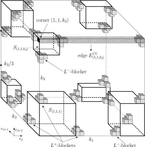
Figure 1. The set $[m_{1}]\times\dots\times[m_{d-1}]\times[k_{1}]\times\dots\times[k_{\ell+1}]$, with examples of blockers and edges. Observe that the $d-1$ first dimensions are not depicted: each ‘unit’ square is a set $\mathcal{M}_{\mathbf{x}}$.

Given vectors $\mathbf{m}\in\mathbb{N}^{d-1}$ and $\mathbf{k}\in\mathbb{N}^{\ell+1}$, we define $C([\mathbf{m}]\times[\mathbf{k}],1)$ to be the bootstrap structure such that

1. the vertex set is $S=[m_{1}]\times\dots\times[m_{d-1}]\times[k_{1}]\times\dots\times[k_{\ell+1}]$,
   

2. the edge set is induced by $\mathbb{Z}^{d+\ell}$,
   

3. $v=(a_{1},\ldots,a_{d-1},b_{1},\ldots,b_{\ell+1})$ has threshold $1+\left|\big{\{}j\in[\ell+1]:b_{j}\not\in\{1,k_{j}\}\big{\}}\right|$.

We remark that in our applications, we shall take $k_{2}=\dots=k_{\ell+1}=k$, and $k_{1}=s$, where $k$ is much larger than $s$.

To study this structure, we slice the set $S=[\mathbf{m}]\times[\mathbf{k}]$ into sets $\mathcal{M}_{\mathbf{x}}$, see Figure 1, where

$$\mathcal{M}_{\mathbf{x}}\;:=\;\big{\{}\mathbf{y}\in[\mathbf{m}]\times[\mathbf{k}]\,:\,y_{d-1+j}=x_{j}\text{ for every }j\in[\ell+1]\big{\}}$$

for each $\mathbf{x}\in[\mathbf{k}]$. Given a vector $\mathbf{x}\in\mathbb{Z}^{d}$, let $\mathcal{C}(\mathbf{x}):=\{1,x_{1}\}\times\dots\times\{1,x_{d}\}$ denote the set of ‘corners’ of $\mathbf{x}$. Now, given a corner $\mathbf{b}\in\mathcal{C}(\mathbf{k})=\{1,k_{1}\}\times\dots\times\{1,k_{\ell+1}\}$ of $S$, and a direction $j\in[\ell+1]$, we define a boundary edge (or simply an edge) of $S$ to be the union of sets $\mathcal{M}_{\mathbf{x}}$ over those $\mathbf{x}$ with $x_{i}=b_{i}$ for $i\neq j$, so

$$E^{(j)}_{\mathbf{b}}\;=\;\bigcup_{t=1}^{k_{j}}\big{\{}\mathcal{M}_{\mathbf{x}}\,:\,x_{i}=b_{i}\textup{ if }i\neq j\textup{ and }x_{j}=t\big{\}}.$$

Note that if $\mathbf{b}_{i}=\mathbf{b}^{\prime}_{i}$ for each $i\neq j$, then $E^{(j)}_{\mathbf{b}}=E^{(j)}_{\mathbf{b}^{\prime}}$.

We shall need the following generalization of the notion of blockers from [6]. Let $e_{i}=(0,\ldots,0,1,0,\ldots,0)$ denote the vector with a single $1$ in position $i$.

Definition.

Given $\mathbf{b}\in\mathcal{C}(\mathbf{k})$ and $j\in[\ell+1]$, let $\mathbf{x}\in E^{(j)}_{\mathbf{b}}$. The set $\mathcal{M}_{\mathbf{x}}$ is an $L^{+}$-blocker of the edge $E^{(j)}_{\mathbf{b}}$ if the events $U_{\mathbf{x}}$ and $\{V_{\mathbf{x}}^{(i)}:d\leqslant i\leqslant d+\ell\}$ all occur, where

$$U_{\mathbf{x}} \,:=\,\big{\{}\mathcal{M}_{\mathbf{x}}\textup{ is not occupied}\big{\}},$$

$$V_{\mathbf{x}}^{(i)} \,:=\,\left\{\begin{array}[]{l}\big{\{}\mathcal{M}_{\mathbf{x}-e_{i}}\textup{ is not occupied}\big{\}}\textup{ if }i\neq j\text{ and }b_{i}=k_{i},\\[4.30554pt] \big{\{}\mathcal{M}_{\mathbf{x}+e_{i}}\textup{ is not occupied}\big{\}}\text{ otherwise}.\end{array}\right.$$

It is an $L^{-}$-blocker of $E^{(j)}_{\mathbf{b}}$ if the event $V_{\mathbf{x}}^{(j)}$ in the definition above is replaced by the event

$$\hat{V}_{\mathbf{x}}^{(j)}\;=\;\{\mathcal{M}_{\mathbf{x}-e_{j}}\textup{ is not occupied}\}.$$

The edge $E^{(i)}_{\mathbf{b}}$ is said to be blocked if there exist $\mathbf{y},\mathbf{z}\in E^{(i)}_{\mathbf{b}}$ such that $\mathcal{M}_{\mathbf{y}}$ is an $L^{+}$-blocker and $\mathcal{M}_{\mathbf{z}}$ is an $L^{-}$-blocker of $E^{(i)}_{\mathbf{b}}$, with $z_{i}>y_{i}$. It is said to be fully blocked if moreover $y_{i}<(k_{i}/3)-1$ and $z_{i}>(2k_{i}/3)+1$.

Note that $L$-blockers are so-named because of their shape; $L$ is not a variable. The following lemma is purely deterministic.

Lemma 7.

Let $\mathbf{m}\in\mathbb{N}^{d-1}$ and $\mathbf{k}\in\mathbb{N}^{\ell+1}$, let $A\subset C([\mathbf{m}]\times[\mathbf{k}],1)$, and let $S=[\mathbf{m}]\times[\mathbf{k}]$. Suppose that there is a path in $[A]$ across $S$ in direction $j$, for some $d\leqslant j\leqslant d+\ell$. Then one of the following holds:

• $A$ contains two sites $x\neq y$ with $d_{G}(x,y)\leqslant 2$.

• One of the boundary edges $\{E^{(j)}_{\mathbf{b}}\,:\,\mathbf{b}\in\mathcal{C}(\mathbf{k})\}$ is not blocked.

• One of the boundary edges $\{E^{(i)}_{\mathbf{b}}\,:\,j\neq i\in[\ell+1],\,\mathbf{b}\in\mathcal{C}(\mathbf{k})\}$ is not fully blocked.

Proof.

Suppose that none of the three events holds; that is, $A\subset S$ does not contain two sites at distance at most two from one another, and for every $\mathbf{b}\in\mathcal{C}(\mathbf{k})$, the boundary edge $E^{(j)}_{\mathbf{b}}$ is blocked, and the boundary edges $\{E^{(i)}_{\mathbf{b}}\,:\,j\neq i\in[\ell+1]\}$ are all fully blocked.

We define a set $\hat{S}$ as follows (see Figure 1). For each $\mathbf{b}\in\mathcal{C}(\mathbf{k})$ and $i\in[\ell+1]$, let $y_{i}(\mathbf{b})$ denote the minimal $i$-coordinate of an $L^{+}$-blocker $\mathcal{M}_{\mathbf{y}}$ of $E^{(i)}_{\mathbf{b}}$, and let $z_{i}(\mathbf{b})$ denote the maximal $i$-coordinate of an $L^{-}$-blocker $\mathcal{M}_{\mathbf{z}}$ of $E^{(i)}_{\mathbf{b}}$. Note that $y_{j}(\mathbf{b})<z_{j}(\mathbf{b})$, and that $y_{i}(\mathbf{b})<(k_{i}/3)-1$ and $z_{i}(\mathbf{b})>(2k_{i}/3)+1$ for every $j\neq i\in[\ell+1]$.

For each $\mathbf{b}\in\mathcal{C}(\mathbf{k})$, let

$$S_{\mathbf{b}}\;:=\;[\mathbf{m}]\times I_{1}(\mathbf{b})\times\dots\times I_{\ell+1}(\mathbf{b}),$$

where $I_{i}(\mathbf{b})=[1,y_{i}(\mathbf{b})-1]$ if $\mathbf{b}_{i}=1$, and $I_{i}(\mathbf{b})=[z_{\ell+1}(\mathbf{b})+1,k_{i}]$ if $\mathbf{b}_{i}=k_{i}$. Let

$$\hat{S}\;:=\;\bigcup_{\mathbf{b}}S_{\mathbf{b}}.$$

Claim: $\hat{S}\cup A$ is a stable set, i.e., $[\hat{S}\cup A]=\hat{S}\cup A$.

Proof of claim.

We first claim that the sets $S_{\mathbf{b}}$ are pairwise at distance at least three. Indeed, let $\mathbf{b},\mathbf{b}^{\prime}\in\mathcal{C}(\mathbf{k})$, and suppose that there exists some $\mathbf{x}\in[\mathbf{k}]$ such that $d(S_{\mathbf{b}},\mathcal{M}_{\mathbf{x}})\leqslant 1$ and $d(S_{\mathbf{b}^{\prime}},\mathcal{M}_{\mathbf{x}})\leqslant 1$. Suppose first that $\mathbf{b}_{i}=\mathbf{b}^{\prime}_{i}$ for every $i\neq j$. Then either $\mathbf{b}=\mathbf{b}^{\prime}$, or $\mathbf{b}_{j}=1$ and $\mathbf{b}^{\prime}_{j}=k_{j}$, say. But then $d(S_{\mathbf{b}},\mathcal{M}_{\mathbf{x}})\leqslant 1$ implies that $\mathbf{x}_{j}\leqslant y_{j}(\mathbf{b})$, and $d(S_{\mathbf{b}^{\prime}},\mathcal{M}_{\mathbf{x}})\leqslant 1$ implies that $\mathbf{x}_{j}\geqslant z_{j}(\mathbf{b})$. Since $y_{j}(\mathbf{b})<z_{j}(\mathbf{b})$, this is a contradiction.

So assume that $\mathbf{b}_{i}=1$ and $\mathbf{b}^{\prime}_{i}=k_{i}$ for some $i\neq j$. Since $d(S_{\mathbf{b}},\mathcal{M}_{\mathbf{x}})\leqslant 1$, we have $\mathbf{x}_{i}\leqslant y_{i}(\mathbf{b})$, and since $d(S_{\mathbf{b}^{\prime}},\mathcal{M}_{\mathbf{x}})\leqslant 1$, we have $\mathbf{x}_{i}\geqslant z_{i}(\mathbf{b}^{\prime})$. But $y_{i}(\mathbf{b})<(k_{i}/3)-1<(2k_{i}/3)+1<z_{i}(\mathbf{b}^{\prime})$, which is a contradiction, and hence the sets $S_{\mathbf{b}}$ are pairwise at distance at least three, as claimed.

Suppose that $[\hat{S}\cup A]\setminus\hat{S}\cup A$ is non-empty, and consider the first new site $v$ to be infected. It has at most one neighbour in $\hat{S}$, by the previous observation, and at most one neighbour in $A$, since $A$ does not contain two sites at distance at most two. Thus $v$ must have threshold at most two, and hence it belongs to an edge, $E^{(i)}_{\mathbf{b}}$, say.

Now, simply note that if a vertex of $E^{(i)}_{\mathbf{b}}$ is at distance one from $\hat{S}$, then it is in $\mathcal{M}_{\mathbf{y}}$ for some $\mathcal{M}_{\mathbf{y}}$ which is a blocker of $E^{(i)}_{\mathbf{b}}$. By the definition of a blocker, these vertices have no element of $A\setminus\hat{S}$ as a neighbour, and so it must have threshold one. But if $v$ has threshold one, then $v\in\mathcal{M}_{\mathbf{b}}$ for some $\mathbf{b}\in\mathcal{C}(\mathbf{k})$, and since $v\not\in\hat{S}$ (by assumption), it follows that $S_{\mathbf{b}}$ is empty, and that $\mathcal{M}_{\mathbf{b}}$ is a blocker for $E^{(i)}_{\mathbf{b}}$, so $v$ has no neighbour in $\hat{S}\cup A$. This final contradiction proves the claim. ∎

It follows immediately from the claim that $[A]\subset\hat{S}\cup A$. But there is no path in $\hat{S}\cup A$ across $S$ in direction $j$, since the rectangles $S_{\mathbf{b}}$ are pairwise at distance at least three, and the elements of $A$ are pairwise at distance at least three. The lemma follows. ∎

We shall need the following bound on the probability that an edge is blocked.

Lemma 8.

Given $\mathbf{m}\in\mathbb{N}^{d-1}$ and $\mathbf{k}\in\mathbb{N}^{\ell+1}$, let $S=C([\mathbf{m}]\times[\mathbf{k}],1)$. Let $\mathbf{b}\in\mathcal{C}(\mathbf{k})$, and let $j\in[\ell+1]$ and $p>0$. Then

$$\mathbb{P}_{p}(E^{(j)}_{\mathbf{b}}\textup{ is not blocked})\;\leqslant\;k_{j}\Big{(}\beta_{\ell+1}\big{(}u(S)\big{)}\Big{)}^{k_{j}-2},$$

and

$$\mathbb{P}_{p}(E^{(j)}_{\mathbf{b}}\textup{ is not fully blocked})\;\leqslant\;2\Big{(}\beta_{\ell+1}\big{(}u(S)\big{)}\Big{)}^{k_{j}/3-2},$$

where $u(S)=u\big{(}\prod_{i=1}^{d-1}m_{i}\big{)}$.

In order to prove Lemma 8, we shall need the following lemma from [6], which is easily proved by induction on $m$. Given $\ell,m\in\mathbb{N}$, consider some sequence of events

$$\mathcal{E}\;=\;\Big{\{}U_{i}:i\in[m+1]\Big{\}}\cup\Big{\{}V^{(i)}_{j}:i\in[\ell],j\in[m]\Big{\}}.$$

An $L$-gap in $\mathcal{E}$ is an event $\neg\left(U_{i}\vee U_{i+1}\vee V^{(1)}_{i}\vee\ldots\vee V^{(\ell)}_{i}\right)$ for some $i\in[m]$.

Lemma 9 (Lemma 6 of [6]).

Let $\ell,m\in\mathbb{N}$, let $u\in(0,1)$, and suppose that each event in the set

$$\mathcal{E}\;=\;\Big{\{}U_{i}:i\in[m+1]\Big{\}}\cup\left\{V^{(i)}_{j}:i\in[\ell],j\in[m]\right\}$$

occurs independently with probability $u$.

Let $L(m,u)$ denote the probability that there is no $L$-gap in $\mathcal{E}$. Then

$$\beta_{\ell+1}(u)^{m+1}\;\leqslant\;L(m,u)\;\leqslant\;\beta_{\ell+1}(u)^{m},$$

where $\beta_{\ell+1}(u)$ is the function defined in the Introduction.

Proof of Lemma 8.

Assume without loss that $\mathbf{b}_{j}=1$, and let $\mathbf{x}(t)=\mathbf{b}+(t-1)e_{j}$ for each $t\in[k_{j}]$, so $E^{(j)}_{\mathbf{b}}=\{\mathbf{x}(t):t\in[k_{j}]\}$. For each $y\in[k_{j}]$, consider the following events:

$$F_{1}(y): \mathcal{M}_{\mathbf{x}(t)} L^{+} E^{(j)}_{\mathbf{b}} 1\leqslant t\leqslant y-1$$ is not an -blocker of for each .

$$F_{2}(y): \mathcal{M}_{\mathbf{x}(t)} L^{-} E^{(j)}_{\mathbf{b}} y+2\leqslant t\leqslant k_{j}$$ is not an -blocker of for each .

Note that the events $F_{1}(y)$ and $F_{2}(y)$ are independent.

Suppose that $E^{(j)}_{\mathbf{b}}$ is not blocked. We claim there exists $y\in[k_{j}]$ such that $F_{1}(y)$ and $F_{2}(y)$ both hold; that is, there is no $L^{+}$-blocker $\mathcal{M}_{\mathbf{x}(t)}$ of $E^{(j)}_{\mathbf{b}}$ with $t<y$, and there is no $L^{-}$-blocker $\mathcal{M}_{\mathbf{x}(t)}$ of $E^{(j)}_{\mathbf{b}}$ with $t>y+1$. (To see this, simply take $y$ minimal such that $\mathcal{M}_{\mathbf{x}(y)}$ is an $L^{+}$-blocker of $E^{(j)}_{\mathbf{b}}$, or $k_{j}$ if there is no such blocker.)

The lemma now follows from Lemma 9, applied to the events $U_{\mathbf{x}(t)}$ and $V_{\mathbf{x}(t)}^{(i)}$ for $t\in[k_{j}]$ and $j\neq i\in[\ell+1]$. Indeed, we have

$$\beta_{\ell+1}\big{(}u(S)\big{)}^{y+1}\;\leqslant\;F_{1}(y)\;\leqslant\;\beta_{\ell+1}\big{(}u(S)\big{)}^{y},$$

and similarly for $F_{2}(y)$, and hence

$$\mathbb{P}_{p}(E^{(j)}_{\mathbf{b}}\textup{ is not blocked})\;\leqslant\;\sum_{y=1}^{k_{j}}\mathbb{P}_{p}\big{(}F_{1}(y)\wedge F_{2}(y)\big{)}\;\leqslant\;k_{j}\Big{(}\beta_{\ell+1}\big{(}u(S)\big{)}\Big{)}^{k_{j}-2},$$

as required.

Finally, if $E^{(j)}_{\mathbf{b}}$ is not fully blocked then either the event $F_{1}\big{(}(k_{j}/3)-1\big{)}$ or the event $F_{2}\big{(}(2k_{j})/3\big{)}$ occurs, and so

$$\mathbb{P}_{p}(E^{(j)}_{\mathbf{b}}\textup{ is not fully blocked}) \leqslant \mathbb{P}_{p}\Big{(}F_{1}\big{(}(k_{j}/3)-1\big{)}\Big{)}\,+\,\mathbb{P}_{p}\Big{(}F_{2}\big{(}(2k_{j})/3\big{)}\Big{)}$$

$$\leqslant 2\Big{(}\beta_{\ell+1}\big{(}u(S)\big{)}\Big{)}^{k_{j}/3-2},$$

as claimed. ∎

Given a rectangle $S\subset C([n]^{d-1}\times[k]^{\ell+1},1)$, a set $A\subset S$, and a direction $j\in[\ell+1]$, define the event

$$\mathcal{X}^{S}_{j}(A)\;:=\;\big{\{}\textup{there is a path in $[A\cap S]$ across $S$ in direction $d+j-1$}\big{\}}.$$

The following upper bound on the probability of $\mathcal{X}^{S}_{j}(A)$ follows easily from Lemmas 7 and 8.

Lemma 10.

Let $B>0$ and $d,k,\ell\in\mathbb{N}$, with $d\geqslant 2$. If $p>0$ is sufficiently small then the following holds. Let $j\in[\ell+1]$, and let $\mathbf{m}\in\mathbb{N}^{d-1}$ and $\mathbf{k}\in\mathbb{N}^{\ell+1}$, with $m_{i}\leqslant B/p^{1/(d-1)}$, $2\ell<k_{j}\leqslant k/6$ and $k/2\leqslant k_{i}\leqslant k$ for each $i\neq j$. Then

$$\mathbb{P}_{p}\big{(}\mathcal{X}^{S}_{j}(A)\big{)}\;\leqslant\;2^{\ell+1}k_{j}\Big{(}\beta_{\ell+1}\big{(}u(S)\big{)}\Big{)}^{k_{j}-2},$$

where $S=C([\mathbf{m}]\times[\mathbf{k}],1)$ and $u(S)=u\big{(}\prod_{i=1}^{d-1}m_{i}\big{)}$.

Proof.

By Lemma 7, if there is a path in $[A]$ across $S$ in direction $d+j-1$, then either $A$ contains two sites within distance two, or one of the boundary edges in direction $j$ is not blocked, or one of the other boundary edges is not fully blocked. The probability that $A$ contains two sites at distance at most two is at most

$$(2d+2\ell)^{2}|S|p^{2}\;\leqslant\;4(d+\ell)^{2}B^{d-1}k^{\ell+1}p\;=\;O(p).$$

There are $2^{\ell}$ boundary edges in direction $j$, so, by Lemma 8, the probability that one of them is not blocked is at most

$$2^{\ell}k_{j}\Big{(}\beta_{\ell+1}\big{(}u(S)\big{)}\Big{)}^{k_{j}-2}.$$

Finally, there are at most $2^{\ell}\ell$ boundary edges not in direction $j$, so the probability that one of them is not fully blocked is at most

$$2^{\ell+1}\ell\Big{(}\beta_{\ell+1}\big{(}u(S)\big{)}\Big{)}^{k/6-2},$$

by Lemma 8, and since $k_{i}\geqslant k/2$ for every $i\neq j$. Since $p$ was chosen sufficiently small, and $k_{j}\leqslant k/6$ and $k_{j}>2\ell$, it follows that

$$\mathbb{P}\big{(}\mathcal{X}^{S}_{j}(A)\big{)}\;\leqslant\;2^{\ell+1}k_{j}\Big{(}\beta_{\ell+1}\big{(}u(S)\big{)}\Big{)}^{k_{j}-2},$$

as required. ∎

We can now deduce Lemma 6 from Lemma 10.

Proof of Lemma 6.

The lower bound is straightforward, and follows by Lemma 7 of [6], and the second inequality is immediate from the definition. We shall prove the upper bound. Let $R$ be a rectangle as described in the lemma, so $R\subset C([n]^{d}\times[k]^{\ell},2)$ with $\dim(R)=(a_{1},\ldots,a_{d})$, where $a_{i}\leqslant B/p^{1/(d-1)}$ for every $i\neq 1$. Recall that $B,\delta>0$, and that $k\geqslant k_{0}(d,\ell,B,\delta)$ is sufficiently large.

Let $A\sim\textup{Bin}(R,p)$, let $t\in\mathbb{N}$, and let $W\subset R$ with $|W|=t$. We are required to bound from above the probability that there is a path in $[A^{\prime}]$ across $R$ in direction $1$, where $A^{\prime}\;=\;(A\cap R)\,\cup\,\{\mathbf{x}\,:\,x_{1}\leqslant a_{1}-1\}\cup W$.

Let $s=k/10$, $\mathbf{m}=(a_{2},\ldots,a_{d})$ and $\mathbf{k}=(s,k,\ldots,k)\in\mathbb{N}^{\ell+1}$, and assume for simplicity that $s$ divides $a_{1}$. We partition $R$ into $M=a_{1}/s$ blocks $B_{1},\ldots,B_{M}$, where $B_{j}\cong[\mathbf{m}]\times[\mathbf{k}]$ for each $j$, in the obvious way, i.e., so that $B_{j}$ is a translate of $[\mathbf{m}]\times[\mathbf{k}]$. Replace the thresholds in $B_{j}$ with those of $C([\mathbf{m}]\times[\mathbf{k}],1)$, and allow the bootstrap process to occur independently in each block. (By this, we mean that the blocks do not interact with each other.) Denote by $\{A\}(j)$ the closure of $A\cap B_{j}$ under this process, i.e., the closure of $A\cap B_{j}$ in the bootstrap structure $C([\mathbf{m}]\times[\mathbf{k}],1)$.

Let $\{A\}=\bigcup_{j=1}^{M}\{A\}(j)$. The following claim shows that this is a coupling.

Claim: $\{A\}\supset[A^{\prime}]$, where $[A^{\prime}]$ denotes the closure of $A^{\prime}$ in $C([n]^{d}\times[k]^{\ell},2)$.

Proof of claim.

Let $\mathbf{x}$ be a vertex of $B_{j}$, so $\mathbf{x}=(y_{1},x_{2},\ldots,x_{d},y_{2},\ldots,y_{\ell+1})$, where $x_{j}\in[m_{j}]$ and $y_{j}\in[k]$ for each $j\geqslant 2$, and $(j-1)s+1\leqslant y_{1}\leqslant js$. Observe that $\mathbf{x}$ has at most one neighbour in $A^{\prime}\setminus B_{j}$, since such a neighbour must differ from $\mathbf{x}$ in direction 1. Moreover, ‘internal’ vertices of $B_{j}$ (those with $y_{1}\not\in\{(j-1)s+1,js\}$) have no neighbours in $A^{\prime}$ outside $B_{j}$.

In the original system, $C([n]^{d}\times[k]^{\ell},2)$, the threshold of vertex $\mathbf{x}$ was

$$r(\mathbf{x})\;=\;2\,+\,\left|\big{\{}2\leqslant j\leqslant\ell+1:y_{j}\not\in\{1,k\}\big{\}}\right|.$$

In the coupled system, it is $r(\mathbf{x})-1+I[y_{1}\not\in\{(j-1)s+1,js\}]$. It follows that the threshold of no vertex has increased, and the threshold of those vertices which have a neighbour in $A^{\prime}$ outside $B_{j}$ have decreased by one. Thus $\{A\}\supset[A^{\prime}]$, as claimed. ∎

Let $\mathcal{J}\subset[M]$ denote the set of indices $j$ such that $B_{j}\cap W\neq\emptyset$, and recall that $|\mathcal{J}|\leqslant t$. Observe that, by the claim, if $R$ is left-to-right crossed by $A\cup W$ in direction 1, then the event $\mathcal{X}^{B_{j}}_{1}(A)$ occurs for each $j\in[M]\setminus\mathcal{J}$, i.e., there is a path in $\{A\}\cap B_{j}$ across $B_{j}$ in direction 1. Note, moreover, that the events $\mathcal{X}^{B_{j}}_{1}(A)$ for $j\in[M]\setminus\mathcal{J}$ are independent. Hence, by Lemma 10, and recalling that $M=a_{1}/s$ and $|\mathcal{J}|\leqslant t$,

$$\mathbb{P}_{p}\Big{(}R\textup{ is left-to-right crossed by }A\text{ in direction }1\>\big{|}\>W\subset A\Big{)}\;\leqslant\;\prod_{j\in[M]\setminus\mathcal{J}}\mathbb{P}_{p}\big{(}\mathcal{X}^{B_{j}}_{1}(A)\big{)}$$

$$\hskip 91.04872pt\;\leqslant\;\prod_{j\in[M]\setminus\mathcal{J}}2^{\ell+1}s\Big{(}\beta_{\ell+1}\big{(}u_{1}(B_{j})\big{)}\Big{)}^{s-2}\;\leqslant\;\Big{(}\beta_{\ell+1}\big{(}u_{1}(B_{j})\big{)}\Big{)}^{(1-\delta)a_{1}-st},$$

where $u_{1}(B_{j})=u\big{(}\prod_{i=2}^{d}a_{i}\big{)}$. In the final inequality we used the fact that $a_{i}\leqslant B/p$ for each $i\neq 1$, so $\beta_{\ell+1}\big{(}u_{1}(B_{j})\big{)}$ is bounded away from 1 (as a function of $B$, $d$ and $\ell$). Hence

$$\Big{(}2^{\ell+1}s\Big{)}^{a_{1}/s}\Big{(}\beta_{\ell+1}\big{(}u_{1}(B_{j})\big{)}\Big{)}^{-2a_{1}/s}\;\leqslant\;\Big{(}\beta_{\ell+1}\big{(}u_{1}(B_{j})\big{)}\Big{)}^{-\delta a_{1}}$$

since $s=k/10$ is sufficiently large. This proves Lemma 6. ∎

6. Analytic tools

In this section we shall extend the analytic tools used by Holroyd [31] to the $d$-dimensional setting. We remark that the results of this section, together with the method of [31], are sufficient to prove Theorem 1 in the case $r=2$.

The following line integral was introduced in [31] in the case $d=2$. Let $\mathbb{R}_{+}$ denote the (strictly) positive reals. Given any function $f:\mathbb{R}_{+}\to\mathbb{R}_{+}$, and $\mathbf{a},\mathbf{b}\in\mathbb{R}^{d}_{+}$, define

$$W_{f}(\mathbf{a},\mathbf{b})\;:=\;\displaystyle\inf_{\gamma\,:\,\mathbf{a}\to\mathbf{b}}\int_{\gamma}\bigg{(}\sum_{j}f\Big{(}\prod_{i\neq j}x_{i}\Big{)}\,\textup{d}x_{j}\bigg{)},$$

where the infimum is taken over all piecewise linear, increasing paths from $\mathbf{a}$ to $\mathbf{b}$ in $\mathbb{R}^{d}_{+}$ (see Section 6 of [31]). Moreover, for any two rectangles $R\subset R^{\prime}\subset[n]^{d}\times[k]^{\ell}$, let

$$U_{f}(R,R^{\prime})\;=\;W_{f}\Big{(}p^{1/(d-1)}\dim(R),p^{1/(d-1)}\dim(R^{\prime})\Big{)}.$$ (3)

The aim of this section is to prove the following two propositions, which will allow us to deduce Theorem 2 from Lemmas 5 and 6. The first is a generalization of Lemma 37 of [31].

Proposition 11.

Let $n,d,k,\ell\in\mathbb{N}$, let $\hat{T},\hat{Z},p>0$, and let $Z=\hat{Z}\cdot p^{1/(d-1)}$. For any hierarchy $\mathcal{H}$ of a rectangle $R\subset C([n]^{d}\times[k]^{\ell},2)$ which is good for $(\hat{T},\hat{Z})$, there exists a rectangle $S=S(\mathcal{H})\subset R$, with

$$\phi(S)\;\leqslant\;\sum_{\textup{seeds }u}\phi(R_{u}),$$

such that

$$\sum_{N_{G_{\mathcal{H}}}^{\rightarrow}(u)=\{v\}}U_{g_{\ell+1}}(R_{v},R_{u})\;\geqslant\;U_{g_{\ell+1}}(S,R)\>-\>\Big{(}d\,p^{1/(d-1)}g_{\ell+1}(Z)\Big{)}\left|\left\{u\in\mathcal{H}:|N_{G_{\mathcal{H}}}^{\rightarrow}(u)|\geqslant 2\right\}\right|.$$

The rectangle $S(\mathcal{H})$ is called the pod of the hierarchy $\mathcal{H}$. In order to understand this statement, ignore the final (error) term, and observe that the lemma gives us a lower bound on the sum a large number of small line integrals (which correspond to events $D(R_{v},R_{u})$ in the hierarchy).

The next result, which is a generalization of Proposition 14 of [31], shows that, if there are not too many big seeds, then this lower bound is exactly what we want. It will follow from the fact that the line integral $W_{g_{\ell}}(\mathbf{a},\mathbf{b})$ is minimized by following the main diagonal as closely as possible.

Given a vector $\mathbf{x}\in\mathbb{R}^{d}$, we shall write $\Delta(\mathbf{x})=\max_{j}\{x_{j}\}$. Given two vectors $\mathbf{a},\mathbf{b}\in\mathbb{R}^{d}$, we shall write $\mathbf{a}\leqslant\mathbf{b}$ if $a_{j}\leqslant b_{j}$ for each $j\in[d]$, and $\mathbf{a}<\mathbf{b}$ if $a_{j}<b_{j}$ for every $j\in[d]$.

Proposition 12.

Let $d,\ell\in\mathbb{N}$, and let $\mathbf{a},\mathbf{b}\in\mathbb{R}^{d}_{+}$, with $\mathbf{a}\leqslant\mathbf{b}$ and $\min_{j}\{b_{j}\}=b_{i}$. Then

$$W_{g_{\ell}}(\mathbf{a},\mathbf{b})\;\geqslant\;d\int_{\Delta(\mathbf{a})}^{\Delta(\mathbf{b})}g_{\ell}(z^{d-1})\,\textup{d}z\;-\;d\Delta(\mathbf{b})g_{\ell}\Big{(}\prod_{i\neq j}b_{j}\Big{)}.$$

Remark 2.

We shall use the following simple properties of the function $g_{k}(z)$ defined in the introduction: $g_{k}(u)$ is decreasing, convex and continuous, and $g_{k}(z)\leqslant 2e^{-kz}$ if $z$ is sufficiently large. Note that either we have $\prod_{i\neq j}b_{j}\leqslant\log\big{(}d\Delta(\mathbf{b})\big{)}$, or $d\Delta(\mathbf{b})g_{k}\big{(}\prod_{i\neq j}b_{j}\big{)}\to 0$ as $\Delta(\mathbf{b})\to\infty$.

We shall prove Propositions 11 and 12 using a discretization argument. Given a function $f$ and a path $\gamma$ in $\mathbb{R}^{d}_{+}$, we shall write

$$w_{f}(\gamma)\;:=\;\int_{\gamma}\bigg{(}\sum_{j}f\Big{(}\prod_{i\neq j}x_{i}\Big{)}\,\textup{d}x_{j}\bigg{)},$$

so that $W_{f}(\mathbf{a},\mathbf{b})=\displaystyle\inf_{\gamma\,:\,\mathbf{a}\to\mathbf{b}}w_{f}(\gamma)$. We begin with a simple observation.

Observation 13.

Let $f:\mathbb{R}_{+}\to\mathbb{R}_{+}$ be continuous, and let $\mathbf{a},\mathbf{b}\in\mathbb{R}^{d}_{+}$ with $\mathbf{0}<\mathbf{a}\leqslant\mathbf{b}$. For every $\varepsilon>0$, there exists a piecewise linear, increasing path $\gamma_{\varepsilon}$ from $\mathbf{a}$ to $\mathbf{b}$, with each linear piece parallel to one of the axes, and all of equal length, such that

$$w_{f}\big{(}\gamma_{\varepsilon}\big{)}\;\leqslant\;W_{f}(\mathbf{a},\mathbf{b})+\varepsilon.$$

The following lemma is a generalization of Lemma 18 of [31].

Lemma 14.

Let $f:\mathbb{R}_{+}\to\mathbb{R}_{+}$ be continuous and decreasing, and let $\mathbf{a},\mathbf{b},\mathbf{c}\in\mathbb{R}^{d}_{+}$ with $\mathbf{a}\leqslant\mathbf{b}\leqslant\mathbf{c}$. Then

$$W_{f}(\mathbf{a},\mathbf{c})\;\geqslant\;W_{f}(\mathbf{b},\mathbf{c}).$$

Remark 3.

Notice that a similarly ‘intuitive’ inequality, that $W_{f}(\mathbf{a},\mathbf{b})\leqslant W_{f}(\mathbf{a},\mathbf{c})$, is not true in general, even in two dimensions. To see this, consider for example the triple $\mathbf{a}=(1,1)$, $\mathbf{b}=(B,1)$ and $\mathbf{c}=(B,B)$, and let $B\gg 1$. Then $W_{f}(\mathbf{a},\mathbf{b})\to\infty$ as $B\to\infty$, but if $f$ is integrable then $W_{f}(\mathbf{a},\mathbf{c})=O(1)$.

Proof.

The proof will be by induction on $d$. When $d=1$ it is trivial, since there is a unique path from $\mathbf{a}$ to $\mathbf{c}$, which passes through $\mathbf{b}$.

Let $d\geqslant 2$, and assume that the result holds for $d-1$. Let $\varepsilon>0$, and let $\gamma_{\varepsilon}$ be the path from $\mathbf{a}$ to $\mathbf{c}$ given by Observation 13. In other words, $\gamma_{\varepsilon}$ is piecewise linear and increasing, with each linear piece parallel to one of the axes, and all of equal length, and $w_{f}(\gamma_{\varepsilon})\leqslant W_{f}(\mathbf{a},\mathbf{c})+\varepsilon$.

Now consider the first point $\mathbf{v}$ on $\gamma_{\varepsilon}$ such that $\mathbf{v}\geqslant\mathbf{b}$, and observe that $\mathbf{v}_{j}=\mathbf{b}_{j}$ for some $j\in[d]$. Assume that $j=1$, let $\mathbf{a}^{\prime}=(b_{1},a_{2},\ldots,a_{d})$, and observe that $\mathbf{a}^{\prime}$, $\mathbf{b}$ and $\mathbf{v}$ all live in the same $(d-1)$-dimensional hyperplane. Hence, by the induction hypothesis, it follows that $W_{f}(\mathbf{a}^{\prime},\mathbf{v})\geqslant W_{f}(\mathbf{b},\mathbf{v})$.

Now, let $\gamma_{1}$ denote the section of $\gamma_{\varepsilon}$ between $\mathbf{a}$ and $\mathbf{v}$, and let $\gamma_{2}$ denote the section from $\mathbf{v}$ to $\mathbf{c}$. Consider the path $\delta_{1}$ from $\mathbf{a}^{\prime}$ to $\mathbf{v}$ obtained from $\gamma_{1}$ by projecting onto the hyperplane $x_{1}=b_{1}$. Observe that each linear piece which is parallel to the $x_{1}$-axis disappears, and each other piece retains its length and direction, and has its $x_{1}$-coordinate increased. Since $f$ is decreasing, it follows that $w_{f}(\delta_{1})\leqslant w_{f}(\gamma_{1})$.

Now, since $W_{f}(\mathbf{a}^{\prime},\mathbf{v})\geqslant W_{f}(\mathbf{b},\mathbf{v})$, it follows that there exists a path $\delta^{\prime}$ from $\mathbf{b}$ to $\mathbf{v}$ such that $w_{f}(\delta^{\prime})\leqslant w_{f}(\delta_{1})+\varepsilon$.

Finally, let $\delta_{\varepsilon}$ denote the path from $\mathbf{a}^{\prime}$ to $\mathbf{c}$ obtained by conjoining the paths $\delta^{\prime}$ (from $\mathbf{b}$ to $\mathbf{v}$) and $\gamma_{2}$ (from $\mathbf{v}$ to $\mathbf{c}$). By the observations above, we have

$$w_{f}\big{(}\delta_{\varepsilon}\big{)}\;\leqslant\;w_{f}(\delta_{1})+w_{f}(\gamma_{2})+\varepsilon\;\leqslant\;w_{f}(\gamma_{1})+w_{f}(\gamma_{2})+\varepsilon\;=\;w_{f}\big{(}\gamma_{\varepsilon}\big{)}+\varepsilon,$$

and hence

$$W_{f}(\mathbf{b},\mathbf{c})\;\leqslant\;w_{f}\big{(}\delta_{\varepsilon}\big{)}\;\leqslant\;w_{f}\big{(}\gamma_{\varepsilon}\big{)}+\varepsilon\;\leqslant\;W_{f}(\mathbf{a},\mathbf{c})+2\varepsilon,$$

by our choice of $\gamma_{\varepsilon}$. Since $\varepsilon>0$ was arbitrary, the lemma follows. ∎

We are now ready to prove Proposition 11. The proof is exactly as in [31], except we need to replace Lemma 18 of [31] with Lemma 14, above. For completeness, we sketch the proof.

Proof of Proposition 11.

Let $f:\mathbb{R}_{+}\to\mathbb{R}_{+}$ be continuous and decreasing; the lemma holds for any such function. The key step is a $d$-dimensional version of Proposition 15 of [31], which states the following: for every $\mathbf{a},\mathbf{b},\mathbf{c},\mathbf{d}\in\mathbb{R}^{d}_{+}$ with $\mathbf{a}\leqslant\mathbf{b}$ and $\mathbf{c}\leqslant\mathbf{d}$, and every $x,Z\in\mathbb{R}_{+}$ and $\mathbf{r}\in\mathbb{R}^{d}_{+}$ with $\mathbf{b},\mathbf{d}\leqslant\mathbf{r}\leqslant\mathbf{b}+\mathbf{d}+(x,\ldots,x)$, $x<Z$ and $\mathbf{r}\geqslant(2Z,\ldots,2Z)$, there exists $\mathbf{s}\in\mathbb{R}^{d}_{+}$ with $\mathbf{s}\leqslant\mathbf{a}+\mathbf{c}$ such that

$$W_{f}(\mathbf{a},\mathbf{b})+W_{f}(\mathbf{c},\mathbf{d})\;\leqslant W_{f}(\mathbf{s},\mathbf{r})-(xd)f(Z).$$

This statement for $d=2$ follows by Propositions 12 and 13 and Lemmas 17 and 18 of [31]. The first three generalize easily to the $d$-dimensional setting; in fact they are easy consequences of the fact that $f$ is decreasing. The last follows for general $d$ by Lemma 14.

Proposition 11 now follows by a straightforward induction argument, exactly as in the proof of Lemma 37 of [31], noting that if $R$, $S$ and $T$ are rectangles with $R=\langle S\cup T\rangle$ in $C([n]^{d}\times[k]^{\ell},2)$, then $\dim(S)+\dim(T)\geqslant\dim(R)-(1,\ldots,1)$. ∎

Finally, we prove Proposition 12. In this case the proof does not follow by the method of [31], which was via an application of Green’s Theorem in the plane. We shall discretize and apply Lemma 15. Given two piecewise linear paths $\gamma$ and $\gamma^{\prime}$ in $\mathbb{R}^{d}_{+}$, we say that $\gamma^{\prime}$ is a permutation of $\gamma$ if it is obtained by permuting the linear pieces of $\gamma$.

The following lemma allows us to permute adjacent linear pieces in order to move the path closer to the main diagonal.

Lemma 15.

Let $f:\mathbb{R}_{+}\to\mathbb{R}_{+}$ be convex, let $\mathbf{a}\in\mathbb{R}^{d}_{+}$ and $b\in\mathbb{R}_{+}$, and set $\mathbf{b}=\mathbf{a}+be_{1}$ and $\mathbf{c}=\mathbf{a}+be_{2}$. Suppose that $a_{1}\leqslant a_{2}$. Then

$$W_{f}(\mathbf{a},\mathbf{b})+W_{f}(\mathbf{b},\mathbf{b}+\mathbf{c})\;\leqslant\;W_{f}(\mathbf{a},\mathbf{c})+W_{f}(\mathbf{c},\mathbf{b}+\mathbf{c}).$$

Proof.

This follows easily from the definition. Since $f$ convex, we have

$$f(x)-f(x+z)\;\leqslant\;f(y)-f(y+z)$$

for any $x,y,z\in\mathbb{R}$ with $x\geqslant y$. Thus

$$W_{f}(\mathbf{a},\mathbf{b})+W_{f}(\mathbf{b},\mathbf{b}+\mathbf{c})\;=\;bf\Big{(}a_{2}\prod_{i\geqslant 3}a_{i}\Big{)}\,+\,bf\Big{(}(a_{1}+b)\prod_{i\geqslant 3}a_{i}\Big{)}$$

$$\hskip 56.9055pt\leqslant\;bf\Big{(}(a_{2}+b)\prod_{i\geqslant 3}a_{i}\Big{)}\,+\,bf\Big{(}a_{1}\prod_{i\geqslant 3}a_{i}\Big{)}\;=\;W_{f}(\mathbf{a},\mathbf{c})+W_{f}(\mathbf{c},\mathbf{b}+\mathbf{c}),$$

by the inequality above with $x=\prod_{i\neq 1}a_{i}$, $y=\prod_{i\neq 2}a_{i}$, and $z=b\prod_{i\geqslant 3}a_{i}$. ∎

Proof of Proposition 12.

Let $f:\mathbb{R}_{+}\to\mathbb{R}_{+}$ be continuous and convex; the result will hold for any such function. Recall that $\mathbf{a},\mathbf{b}\in\mathbb{R}^{d}_{+}$ with $\mathbf{a}\leqslant\mathbf{b}$, and assume without loss of generality that $b_{1}\leqslant\ldots\leqslant b_{d}$. We require a lower bound on $W_{f}(\mathbf{a},\mathbf{b})$. Let $B=b_{d}=\Delta(\mathbf{b})$ and let $\mathbf{b}^{\prime}=(B,\ldots,B)$. Observe that $\mathbf{b}^{\prime}\geqslant\mathbf{b}$, so

$$W_{f}(\mathbf{a},\mathbf{b}^{\prime})\;\leqslant\;W_{f}(\mathbf{a},\mathbf{b})\,+\,W_{f}(\mathbf{b},\mathbf{b}^{\prime}).$$

It is easy to see that $W_{f}(\mathbf{b},\mathbf{b}^{\prime})\leqslant(Bd)f\big{(}\prod_{j=2}^{d}b_{j}\big{)}=d\Delta(\mathbf{b})f\big{(}\prod_{j=2}^{d}b_{j}\big{)}$ (simply choose a path which grows in direction 1 first, then direction 2, and so on), and so the proposition will follow from the statement

$$W_{f}(\mathbf{a},\mathbf{b}^{\prime})\;\geqslant\;d\int_{\Delta(\mathbf{a})}^{B}f(z^{d-1})\,\textup{d}z.$$

Let $\varepsilon>0$, and let $\gamma$ be a path from $\mathbf{a}$ to $\mathbf{b}^{\prime}=(B,\ldots,B)$ given by Observation 13. Thus $\gamma$ is piecewise linear and increasing, with each linear piece parallel to one of the axes, and all of equal length, and $w_{f}(\gamma)\leqslant W_{f}(\mathbf{a},\mathbf{b}^{\prime})+\varepsilon$. Let $\delta>0$ denote the length of each piece of $\gamma$, and note that we may choose $\delta$ as small as we like.

We claim that there exists a permutation $\gamma^{\prime}$ of $\gamma$ which passes within $\ell_{\infty}$-distance $\delta$ of every point of the straight line between $(A,\ldots,A)$ and $(B,\ldots,B)$, such that

$$w_{f}(\gamma)\;\geqslant\;w_{f}(\gamma^{\prime})\;\geqslant\;d\int_{\Delta(\mathbf{a})}^{B}f(z^{d-1})\,\textup{d}z\,-\,\varepsilon.$$

This follows by Lemma 15. Indeed, let $\gamma^{\prime}$ be chosen to minimize $w_{f}(\gamma^{\prime})$ over all permutations of $\gamma$. Assume, without loss of generality, that $a_{1}\leqslant a_{2}\leqslant\dots\leqslant a_{d}$, and consider the piecewise linear path $\zeta$, given by

$$(a_{1},\ldots,a_{d})\to\dots\to(a_{j},\ldots,a_{j},a_{j+1},\ldots,a_{d})\to\dots\to(a_{d},\ldots,a_{d})\to(B,\ldots,B),$$

where $\mathbf{x}\to\mathbf{y}$ means that $\zeta$ follows a straight line between $\mathbf{x}$ and $\mathbf{y}$. By Lemma 15, we can choose $\gamma^{\prime}$ to be the permutation which follows $\zeta$ as closely as possible. The second inequality follows because $f$ is continuous, and we chose $\delta>0$ sufficiently small.

Putting the pieces together, we have

$$W_{f}(\mathbf{a},\mathbf{b}^{\prime})\;\geqslant\;w_{f}(\gamma)-\varepsilon\;\geqslant\;w_{f}(\gamma^{\prime})-\varepsilon\;\geqslant\;d\int_{\Delta(\mathbf{a})}^{B}f(z^{d-1})\,\textup{d}z\,-\,2\varepsilon.$$

Since $\varepsilon>0$ was arbitrary, the result follows. ∎

To finish the section, we prove the following simple property of $\lambda(d,r)$, which will be useful in Section 7.

Proposition 16.

Let $d,\ell\in\mathbb{N}$ with $d\geqslant 2$. Then $\lambda(d+\ell,\ell+2)<\displaystyle\frac{d+1}{2}$.

Proof.

Recall from (1) that

$$\lambda(d+\ell,\ell+2)\;=\;\int_{0}^{\infty}g_{\ell+1}(z^{d-1})\,\textup{d}z.$$

By Proposition 3 of [6], we have $g_{k+1}(z)\leqslant g_{k}(z)$ for every $k\in\mathbb{N}$ and $z\in(0,\infty)$, so it suffices to prove the result for $\ell=0$. By Theorem 5 of [33], we have

$$\int_{\log(3/2)}^{\infty}g_{1}(z)\,\textup{d}z\;=\;\int_{0}^{2/3}\frac{-\log\big{(}\beta_{1}(1-x)\big{)}}{x}\,\textup{d}x\;<\;\frac{\pi^{2}}{36}\;<\;\frac{1}{3}.$$

Moreover, since $g_{1}$ is decreasing, we have $g_{1}(z^{d-1})\leqslant g_{1}(z)$ whenever $z\geqslant 1$. Hence

$$\int_{1}^{\infty}g_{1}(z^{d-1})\,\textup{d}z\;\leqslant\;\int_{1}^{\infty}g_{1}(z)\,\textup{d}z\;\leqslant\;\int_{\log(3/2)}^{\infty}g_{1}(z)\,\textup{d}z\;<\;\frac{1}{3}.$$

To bound the integral when $z<1$, observe that $\beta_{1}(u)\geqslant\sqrt{u}$ for $0\leqslant u\leqslant 1$, and that $1-e^{-z}\geqslant(1-1/e)z$ for $0\leqslant z\leqslant 1$, so

$$\beta_{1}(1-e^{-z})\;\geqslant\;\sqrt{1-e^{-z}}\;\geqslant\;\left(1-\frac{1}{e}\right)^{1/2}\sqrt{z}$$

for every $0\leqslant z\leqslant 1$. Hence $g_{1}(z^{d-1})\leqslant-\log\left(z^{(d-1)/2}\right)+\displaystyle\frac{1-\log(e-1)}{2}$, and so

$$\int_{0}^{1}g_{1}(z^{d-1})\,\textup{d}z\;\leqslant\;\frac{d-1}{2}\int_{0}^{1}-\log z\,\textup{d}z\,+\,\frac{2}{5}\;=\;\frac{d-1}{2}\,+\,\frac{2}{5}.$$

Thus $\lambda(d+\ell,\ell+2)\leqslant\displaystyle\frac{d-1}{2}+\frac{2}{5}+\frac{1}{3}<\frac{d+1}{2}$, as claimed. ∎

7. Proof of Theorem 2

In this section we complete the proof of Theorem 2. We shall follow the basic method of Holroyd [31] (see also Sections 4.3 and 4.4 of [6]), but we shall need some new ideas here also. Theorem 2 will follow easily from the following theorem (see Corollary 23).

Theorem 17.

For every $d,\ell\in\mathbb{N}$ with $d\geqslant 2$, and every $\varepsilon>0$, there exists $B_{0}>0$ and $k_{0}:\mathbb{N}\to\mathbb{N}$ such that the following holds for every $B\geqslant B_{0}$ and every $k\geqslant k_{0}(B)$.

Let $G=C([n]^{d}\times[k]^{\ell},2)$, and let $p>0$ be sufficiently small. Let $R\subset V(G)$ be a rectangle with $\textup{long}(R)=B/p^{1/(d-1)}$. Then

$$\mathbb{P}_{p}\big{(}R\in\langle A\cap R\rangle\big{)}\;\leqslant\;\exp\left(-\frac{d\lambda(d+\ell,\ell+2)-\varepsilon}{p^{1/(d-1)}}\right).$$

We begin by bounding the probability that a rectangle grows sideways by $T/p^{1/(d-1)}$. Let $R\subset R^{\prime}$ be rectangles in $C([n]^{d}\times[k]^{\ell},2)$, and recall from Section 4 that $P_{p}(R,R^{\prime})=\mathbb{P}_{p}\big{(}D(R,R^{\prime})\big{)}$, where $D(R,R^{\prime})$ denotes the event that $R^{\prime}$ is internally spanned by $(A\cup R)\cap R^{\prime}$.

We shall deduce the following lemma from Lemma 6. We refer the reader to [28] (see Lemma 5) where a similar trick is used.

Lemma 18.

For each $d,\ell\in\mathbb{N}$ and $B,\delta>0$, there exist constants $k\in\mathbb{N}$, $Z=Z(k)>0$ and $T=T(k,Z)>0$ such that the following holds.

Let $p>0$ be sufficiently small, and let $R\subset R^{\prime}$ be rectangles in $C([n]^{d}\times[k]^{\ell},2)$ with $\dim(R)=(m_{1},\ldots,m_{d})$ and $\dim(R^{\prime})=(m_{1}+s_{1},\ldots,m_{d}+s_{d})$. Suppose that $Z/p^{1/(d-1)}\leqslant m_{j}\leqslant B/p^{1/(d-1)}$ and $s_{j}\leqslant T/p^{1/(d-1)}$ for each $j\in[d]$. Then

$$P_{p}(R,R^{\prime}) \leqslant \exp\bigg{(}-\big{(}1-2\delta\big{)}\sum_{j=1}^{d}g_{\ell+1}\Big{(}q\prod_{i\neq j}m_{i}\Big{)}s_{j}\bigg{)}.$$ (4)

Proof.

For each direction $j\in[d]$, let $R^{<}_{j}$ denote the rectangle $\{\mathbf{x}\in R^{\prime}:x_{j}<y_{j}\textup{ for all }\mathbf{y}\in R\}$, and similarly let $R^{>}_{j}$ denote the rectangle $\{\mathbf{x}\in R^{\prime}:x_{j}>y_{j}\textup{ for all }\mathbf{y}\in R\}$. Write $R_{j}=R^{<}_{j}\cup R^{>}_{j}$, and let $C=\bigcup_{i<j}R_{i}\cap R_{j}$ denote the corner areas of $R^{\prime}\setminus R$. Finally, let $W=A\cap C$, and let $t=|W|$.

If the event $D(R,R^{\prime})$ occurs, then clearly the events $H^{\rightarrow(j)}(R^{>}_{j})$ and $H^{\leftarrow(j)}(R^{<}_{j})$ must also occur for each $j\in[d]$. Hence,

$$P_{p}(R,R^{\prime}) \leqslant \mathbb{P}_{p}\left(\bigwedge_{j}H^{\rightarrow(j)}(R^{>}_{j})\wedge H^{\leftarrow(j)}(R^{<}_{j})\right).$$

Note that $|C|\leqslant{d\choose 2}T^{2}B^{d-2}p^{-d/(d-1)}$. The idea is that, since $T$ may be chosen small compared with $Z$ (and also $B$, $d$, $k$, $\ell$), it is likely that $|A\cap C|$ will be small compared with $s_{j}$, and so the events $H^{\rightarrow(i)}(R^{>}_{i})$ and $H^{\leftarrow(j)}(R^{<}_{j})$ are ‘almost independent’.

To be precise, by Lemma 6, and the binomial theorem, we have

$$P_{p}(R,R^{\prime}) \leqslant \sum_{t=0}^{|C|}{{|C|}\choose t}p^{t}(1-p)^{|C|-t}\prod_{j}h^{(j)}(R^{>}_{j},t)\cdot h^{(j)}(R^{<}_{j},t)$$

$$\leqslant \sum_{t=0}^{|C|}{{|C|}\choose t}p^{t}\prod_{j}\big{(}\beta_{\ell+1}\big{(}u_{j}(R)\big{)}\big{)}^{(1-\delta)s_{j}-kt}$$

$$= \left(\prod_{j}\Big{(}\beta_{\ell+1}\big{(}u_{j}(R)\big{)}\Big{)}^{(1-\delta)s_{j}}\right)\left(1+p\prod_{j}\Big{(}\beta_{\ell+1}\big{(}u_{j}(R)\big{)}\Big{)}^{-k}\right)^{|C|}.$$

To estimate the error term, we use our bounds on $m_{j}$ and $s_{j}$. Indeed, since $m_{j}\geqslant Z/p^{1/(d-1)}$ for each $j\in[d]$, we have $u_{j}(R)\geqslant 1-\exp(-Z^{d-1})\geqslant Z^{d-1}/2$. Since $\beta_{\ell+1}(u)$ is increasing on $[0,1]$ (see Proposition 3 of [6]), and $\beta_{\ell+1}(u)\geqslant u$ when $u$ is small, it follows that

$$\prod_{j}\Big{(}\beta_{\ell+1}\big{(}u_{j}(R)\big{)}\Big{)}^{-k}\;\leqslant\;\prod_{j}\big{(}2/Z^{d-1}\big{)}^{k}\;\leqslant\;\left(\frac{1}{Z}\right)^{kd^{2}}.$$

Let $T_{1}=p^{1/(d-1)}\max_{j}\{s_{j}\}\leqslant T$, and recall that $|C|\leqslant{d\choose 2}T_{1}^{2}B^{d-2}p^{-d/(d-1)}$, since $m_{j}\leqslant B/p^{1/(d-1)}$ for each $j\in[d]$. Hence, since $T_{1}\leqslant T$,

$$\left(1+p\prod_{j}\Big{(}\beta_{\ell+1}\big{(}u_{j}(R)\big{)}\Big{)}^{-k}\right)^{|C|}\;\leqslant\;\exp\Big{(}|C|Z^{-kd^{2}}p\Big{)}\;\leqslant\;\exp\left(\frac{T_{1}^{3/2}}{p^{1/(d-1)}}\right)$$

$$\hskip 85.35826pt\leqslant\;\exp\bigg{(}\delta g_{\ell+1}\big{(}2B^{d-1}\big{)}\max_{j}\{s_{j}\}\bigg{)}\;\leqslant\;\exp\bigg{(}\delta\sum_{j=1}^{d}g_{\ell+1}\Big{(}q\prod_{i\neq j}m_{i}\Big{)}s_{j}\bigg{)},$$

if $T>0$ is chosen to be sufficiently small (with respect to $d$, $\ell$, $B$, $\delta$, $k$ and $Z$). The penultimate inequality follows since we may we choose $\sqrt{T}\leqslant\delta g_{\ell+1}\big{(}2B^{d-1}\big{)}$. In the final inequality, we used the facts that $g_{\ell+1}$ is decreasing, and that $q\prod_{i\neq j}m_{i}\leqslant 2B^{d-1}$.

Finally, recall that $e^{-g_{\ell+1}(qx)}=\beta_{\ell+1}\big{(}u(x)\big{)}$, so

$$\prod_{j}\Big{(}\beta_{\ell+1}\big{(}u_{j}(R)\big{)}\Big{)}^{(1-\delta)s_{j}}\;=\;\exp\bigg{(}-\big{(}1-\delta\big{)}\sum_{j=1}^{d}g_{\ell+1}\Big{(}q\prod_{i\neq j}m_{i}\Big{)}s_{j}\bigg{)}.$$

Combining these bounds, the lemma follows. ∎

We now rewrite the right-hand side of (4) in a more useful form. We shall use the following easy observation from [31].

Observation 19 (Proposition 12 of [31]).

If $f$ is decreasing, then

$$W_{f}(\mathbf{a},\mathbf{b})\;\leqslant\;\sum_{j=1}^{d}\big{(}b_{j}-a_{j}\big{)}f\Big{(}\prod_{i\neq j}a_{i}\Big{)}.$$

By Observation 19 and the definition of $U_{g_{\ell+1}}(R,R^{\prime})$, we have

$$\frac{1}{p^{1/(d-1)}}U_{g_{\ell+1}}(R,R^{\prime})\;\leqslant\;\sum_{j=1}^{d}g_{\ell+1}\Big{(}q\prod_{i\neq j}m_{i}\Big{)}s_{j}.$$

The following corollary of Lemma 18 is now immediate.

Corollary 20.

Under the conditions of Lemma 18,

$$P_{p}(R,R^{\prime})\;\leqslant\;\exp\left(-\big{(}1-2\delta\big{)}\frac{U_{g_{\ell+1}}(R,R^{\prime})}{p^{1/(d-1)}}\right).$$

Next we bound the probability that a seed is internally spanned. Recall that $\phi(R)$ denotes the semi-perimeter of a rectangle $R$.

Lemma 21.

Let $d,\ell,k\in\mathbb{N}$, let $B,\alpha>0$, and let $Z=Z(d,\ell,B,\alpha,k)>0$ be sufficiently small. Let $p>0$, and let $R$ be a rectangle in $C([n]^{d}\times[k]^{\ell},2)$. Suppose $\textup{short}(R)\leqslant Z/p^{1/(d-1)}$ and $\textup{long}(R)\leqslant B/p^{1/(d-1)}$. Then

$$\mathbb{P}_{p}(R\in\langle A\cap R\rangle)\;\leqslant\;e^{-\alpha\phi(R)}.$$

Proof.

Let $\dim(R)=(u_{1},\ldots,u_{d})$, and suppose without loss of generality that $u_{1}=\textup{long}(R)$ and $u_{2}=\textup{short}(R)$. Note that if $R\in\langle A\cap R\rangle$, then $R$ has no ‘double gap’, i.e., no pair of adjacent empty hyperplanes (see Lemma 27 of [6]). Thus,

$$\mathbb{P}\big{(}R\in\langle A\cap R\rangle\big{)}\;\leqslant\;\Big{(}2k^{\ell}u_{1}^{d-2}u_{2}p\Big{)}^{u_{1}/2}\;\leqslant\;\Big{(}2k^{\ell}B^{d-2}Z\Big{)}^{\phi(R)/2d}\;\leqslant\;e^{-\alpha\phi(R)}$$

if $2k^{\ell}B^{d-2}Z\leqslant e^{-2d\alpha}$, which holds if $Z>0$ is sufficiently small, as required. ∎

Finally, we recall the following lemma from [6] (see also [2]).

Lemma 22 (Lemma 16 of [6]).

Let $A\subset C([n]^{d}\times[k]^{\ell},2)$. If $1\leqslant L\leqslant\textup{diam}([A])$, then there exists a rectangle $R$, internally spanned by $A$, with

$$L\;\leqslant\;\textup{long}(R)\;\leqslant\;2L.$$

We are ready to prove Theorem 17.

Proof of Theorem 17.

Let $d,\ell\in\mathbb{N}$, with $d\geqslant 2$, and let $\varepsilon>0$. We choose positive constants $B$, $\alpha$, $\delta$, $k$, $Z$ and $T$ (chosen in that order), with $B>0$ sufficiently large, $\delta>0$ sufficiently small, and $k$, $Z$ and $T$ chosen so that Lemmas 18 and 21 hold. In particular, let $\alpha=d\lambda(d+\ell,\ell+2)B$, and note that

$$T\ll Z\ll\delta\ll 1\ll B\ll k.$$

Finally, we let $p\to 0$, so that $p\ll T$. Let $\hat{T}=T/p^{1/(d-1)}$ and $\hat{Z}=Z/p^{1/(d-1)}$.

Let $R$ be a rectangle in $G=C([n]^{d}\times[k]^{\ell},2)$ with $\dim(R)=(b_{1},\ldots,b_{d})$, let $\textup{long}(R)=B/p^{1/(d-1)}$, and assume without loss of generality that $b_{1}\leqslant\ldots\leqslant b_{d}$. By Corollary 20 and Lemmas 5 and 21, we obtain

$$\mathbb{P}_{p}\big{(}R\in\langle A\cap R\rangle\big{)}\;\leqslant\;\sum_{\mathcal{H}\in\mathcal{H}(R,\hat{T},\hat{Z})}\left(\prod_{N_{G_{\mathcal{H}}}^{\rightarrow}(u)=\{v\}}P_{p}(R_{v},R_{u})\right)\left(\prod_{\textup{ seeds $u\in\mathcal{H}$}}P_{p}(R_{u})\right)$$

$$\hskip 28.45274pt\leqslant\;\sum_{\mathcal{H}\in\mathcal{H}(R,\hat{T},\hat{Z})}\exp\left(-\sum_{N_{G_{\mathcal{H}}}^{\rightarrow}(u)=\{v\}}\frac{(1-2\delta)U_{g_{\ell+1}}(R_{v},R_{u})}{p^{1/(d-1)}}-\alpha\sum_{\textup{seeds $u\in\mathcal{H}$}}\phi(R_{u})\right)$$ (5)

For each hierarchy $\mathcal{H}\in\mathcal{H}(R,\hat{T},\hat{Z})$, let

$$Q(\mathcal{H})\;:=\;\exp\left(-\sum_{N_{G_{\mathcal{H}}}^{\rightarrow}(u)=\{v\}}\frac{(1-2\delta)U_{g_{\ell+1}}(R_{v},R_{u})}{p^{1/(d-1)}}-\alpha\sum_{\textup{seeds $u\in\mathcal{H}$}}\phi(R_{u})\right).$$

The theorem will follow easily from (5), Lemma 4 and the following claim.

Claim: $Q(\mathcal{H})\leqslant\exp\left(-\displaystyle\frac{d\lambda(d+\ell,\ell+2)-\varepsilon}{p^{1/(d-1)}}\right)$ for every $\mathcal{H}\in\mathcal{H}(R,\hat{T},\hat{Z})$.

Proof of claim.

We shall consider three cases. First, suppose that $\mathcal{H}$ has ‘many’ seeds.

Case 1: $\displaystyle\sum_{\textup{ seeds }u}\phi(R_{u})\geqslant\displaystyle\frac{1}{Bp^{1/(d-1)}}$.

In this case it is sufficient to consider only the second term in $Q(\mathcal{H})$. Indeed,

$$\exp\left(-\alpha\sum_{\textup{ seeds }u}\phi(R_{u})\right)\;\leqslant\;\exp\left(-\frac{\alpha}{Bp^{1/(d-1)}}\right)\;=\;\exp\left(-\displaystyle\frac{d\lambda(d+\ell,\ell+2)}{p^{1/(d-1)}}\right)$$

if $p>0$ is sufficiently small, since $\alpha=d\lambda(d+\ell,\ell+2)B$, as required.

Next, suppose that $R$ is unusually ‘long and thin’. Let $\textup{girth}(R)=p\prod_{j=2}^{d}b_{j}$, and recall that $b_{d}=B/p^{1/(d-1)}$, and that $B$ is chosen to be sufficiently large.

Case 2: $\displaystyle\sum_{\textup{ seeds }u}\phi(R_{u})\leqslant\displaystyle\frac{1}{Bp^{1/(d-1)}}$ and $\textup{girth}(R)\leqslant 2\log(Bd)$.

In this case we consider only the first term in $Q(\mathcal{H})$. Let $S=S(\mathcal{H})$ be the pod of $\mathcal{H}$, given by Proposition 11. Note that $\mathcal{H}$ has bounded height (in terms of $B$, $d$ and $T$), and hence that $|G_{\mathcal{H}}|$ is bounded (as $p\to 0$). Hence, by Proposition 11, we have

$$Q(\mathcal{H})\;\leqslant\;\exp\left(-\frac{(1-2\delta)U_{g_{\ell+1}}(S,R)}{p^{1/(d-1)}}+M_{1}\right),$$ (6)

for some constant $M_{1}=M_{1}(d,\ell,B,Z,T)$.

Next, note that $b_{d}/b_{1}\geqslant\sqrt{B}$, since $\textup{girth}(R)\leqslant 2\log(Bd)\leqslant\sqrt{B}$ and so

$$b_{1}\;\leqslant\;\left(\frac{\textup{girth}(R)}{p}\right)^{1/(d-1)}\;\leqslant\;\left(\frac{\sqrt{B}}{p}\right)^{1/(d-1)}\;\leqslant\;\frac{\sqrt{B}}{p^{1/(d-1)}},$$

whereas $b_{d}=B/p^{1/(d-1)}$. Recall (3), the definition of $U_{g_{\ell+1}}(S,R)$, and recall also that $\phi(S)\leqslant\sum_{\textup{seeds}}\phi(R_{u})$, and that $g_{\ell+1}$ is decreasing. We obtain

$$U_{g_{\ell+1}}(S,R)\;\geqslant\;\Big{(}B-\phi(S)p^{1/(d-1)}\Big{)}g_{\ell+1}\bigg{(}q\prod_{j=1}^{d-1}b_{j}\bigg{)}\;\geqslant\;\big{(}B-1\big{)}g_{\ell+1}\left(\frac{4\log(Bd)}{\sqrt{B}}\right)\;\geqslant\;2B,$$

if $B>0$ is sufficiently large. The first inequality above follows by considering growth only in direction $d$. For the second step, note that $q\prod_{j=1}^{d-1}b_{j}\leqslant 2\cdot\textup{girth}(R)(b_{1}/b_{d})$, and use the upper bounds on $\sum_{\textup{seeds}}\phi(R_{u})$, $\textup{girth}(R)$ and $b_{1}/b_{d}$. The final inequality holds if $B$ is sufficiently large, since $g_{\ell+1}(z)\to\infty$ as $z\to 0$.

Thus, combining this bound with (6), we deduce that

$$Q(\mathcal{H})\;\leqslant\;\exp\left(-\frac{B}{p^{1/(d-1)}}+M_{1}\right)\;<\;\exp\left(-\frac{d\lambda(d+\ell,\ell+2)}{p^{1/(d-1)}}\right)$$

if $B>0$ is sufficiently large and $p>0$ is sufficiently small, as required.

Finally, we arrive at the main case.

Case 3: $\displaystyle\sum_{\textup{ seeds }u}\phi(R_{u})\leqslant\displaystyle\frac{1}{Bp^{1/(d-1)}}$ and $\textup{girth}(R)\geqslant 2\log(Bd)$.

The inequality (6) again follows from Proposition 11 and the definition of $Q(\mathcal{H})$, exactly as in Case 2. By Proposition 12 (applied to the vectors $\mathbf{a}=p^{1/(d-1)}\dim(S)$ and $\mathbf{b}=p^{1/(d-1)}\dim(R)$), we have

$$U_{g_{\ell+1}}(S,R)\;\geqslant\;d\int_{1/B}^{B}g_{\ell+1}\big{(}z^{d-1}\big{)}\,\textup{d}z\>-\>(Bd)g_{\ell+1}\Big{(}p\prod_{j=2}^{d}b_{j}\Big{)},$$

and hence, recalling that $\textup{girth}(R)\geqslant 2\log(Bd)$ and noting that $\delta/p^{1/(d-1)}\gg M_{1}$,

$$Q(\mathcal{H})\;\leqslant\;\exp\left[-\frac{(1-3\delta)}{p^{1/(d-1)}}\left(d\int_{1/B}^{B}g_{\ell+1}\big{(}z^{d-1}\big{)}\,\textup{d}z\>-\>(Bd)g_{\ell+1}\Big{(}2\log(Bd)\Big{)}\right)\right].$$

But $g_{\ell+1}(z)\leqslant 2e^{-(\ell+1)z}$ for large $z$ (see [6]), so

$$Q(\mathcal{H}) \leqslant \exp\left[-\frac{(1-3\delta)}{p^{1/(d-1)}}\left(d\int_{1/B}^{B}g_{\ell+1}\big{(}z^{d-1}\big{)}\,\textup{d}z\>-\>\frac{2}{Bd}\right)\right]$$

$$\leqslant \exp\left(-\frac{d\lambda(d+\ell,\ell+2)-\varepsilon}{p^{1/(d-1)}}\right)$$

if $B$ is sufficiently large, and $\delta$ is sufficiently small, as required. ∎

To complete the proof of Theorem 17, recall that, by Lemma 4,

$$|\mathcal{H}(R,\hat{T},\hat{Z})|\;\leqslant\;M_{2}\left(\frac{1}{p}\right)^{M_{2}}.$$

for some constant $M_{2}=M_{2}(B,T,d,\ell)$. Hence, by (5) and the claim,

$$\mathbb{P}_{p}\big{(}R\in\langle A\cap R\rangle\big{)}\;\leqslant\;\sum_{\mathcal{H}\in\mathcal{H}(R,\hat{T},\hat{Z})}Q(\mathcal{H})\;\leqslant\;M_{2}\left(\frac{1}{p}\right)^{M_{2}}\max_{\mathcal{H}\in\mathcal{H}(R,\hat{T},\hat{Z})}Q(\mathcal{H})$$

$$\hskip 28.45274pt\leqslant\;M_{2}\left(\frac{1}{p}\right)^{M_{2}}\exp\left(-\displaystyle\frac{d\lambda(d+\ell,\ell+2)-\varepsilon}{p^{1/(d-1)}}\right)\;\leqslant\;\exp\left(-\displaystyle\frac{d\lambda(d+\ell,\ell+2)-2\varepsilon}{p^{1/(d-1)}}\right)$$

if $p>0$ is sufficiently small. Since $\varepsilon>0$ was arbitrary, the theorem follows. ∎

We complete this section by deducing the following corollary of Theorem 17, which is the technical statement which we shall need in Section 9.

Corollary 23.

Let $d,\ell\in\mathbb{N}$, with $d\geqslant 2$. If $\varepsilon>0$ is sufficiently small, then there exist $B>0$ and $k_{0}=k_{0}(B)>0$ such that, if $k\geqslant k_{0}$ and $n\geqslant n_{0}(B,d,k,\ell,\varepsilon)$ is sufficiently large, then the following holds. Let $G=C([n]^{d}\times[k]^{\ell},2)$, and let

$$p\,=\,p(n)\,\leqslant\,\left(\displaystyle\frac{\lambda(d+\ell,\ell+2)-\varepsilon}{\log n}\right)^{d-1}.$$

Then

$$\mathbb{P}_{p}\Big{(}\textup{diam}([A])\geqslant B\log n\Big{)}\;\leqslant\;n^{-\varepsilon}.$$

Proof.

Let $\varepsilon^{\prime}=\varepsilon^{\prime}(d,\ell,\varepsilon)>0$ be sufficiently small, let $B_{0}=B_{0}(\varepsilon^{\prime})$, $k_{0}=k_{0}(B_{0},\varepsilon^{\prime})$ be chosen according to Theorem 17, and write $\lambda=\lambda(d+\ell,\ell+2)$. Let $n\in\mathbb{N}$ and, noting that the probability is monotone in $p$, let

$$p\,=\,p(n)\,=\,\left(\displaystyle\frac{\lambda-\varepsilon}{\log n}\right)^{d-1}.$$

Let $B_{1}=2B_{0}/(\lambda-\varepsilon)$. We shall show that

$$\mathbb{P}_{p}\Big{(}\textup{long}(R)\geqslant B_{1}\log n\textup{ for some }R\in\langle A\rangle\Big{)}\;\leqslant\;n^{-\varepsilon}.$$

The result will then follow, since $\textup{diam}([A])\leqslant\max\big{\{}\textup{long}(R):R\in\langle A\rangle\big{\}}$.

Suppose $\textup{long}(R)\geqslant B_{1}\log n$ for some $R\in\langle A\rangle$. By Lemma 22, there exists an internally spanned rectangle $R^{\prime}\subset R$ with

$$\frac{B_{1}\log n}{2}\;\leqslant\;\textup{long}(R^{\prime})\;\leqslant\;B_{1}\log n.$$

By our choice of $p$, it follows that $\textup{long}(R^{\prime})=B/p^{1/(d-1)}$ for some $B\in[B_{0},2B_{0}]$. Hence, by Theorem 17, if $n$ is sufficiently large then

$$\mathbb{P}_{p}\big{(}R^{\prime}\in\langle A\cap R^{\prime}\rangle\big{)}\;\leqslant\;\exp\left(-\frac{d\lambda-\varepsilon^{\prime}}{p^{1/(d-1)}}\right)\;\leqslant\;\exp\left(-\left(\frac{d\lambda-\varepsilon^{\prime}}{\lambda-\varepsilon}\right)\log n\right)\;\leqslant\;n^{-(d+\varepsilon+\varepsilon^{\prime})}.$$

The last inequality holds since $\varepsilon>0$ and $\varepsilon^{\prime}=\varepsilon^{\prime}(d,\ell,\varepsilon)>0$ were chosen sufficiently small, and because $\lambda(d+\ell,\ell+2)<(d+1)/2<d$, by Proposition 16.

There are at most $(B\log n)^{d}n^{d}\leqslant n^{d+\varepsilon^{\prime}}$ potential such rectangles $R^{\prime}$. So, writing $Y(B_{1})$ for the number of internally spanned rectangles $R^{\prime}\subset C([n]^{d}\times[k]^{\ell},2)$ with $(B_{1}/2)\log n\leqslant\textup{long}(R^{\prime})\leqslant B_{1}\log n$, we get

$$\mathbb{P}_{p}\big{(}\textup{long}(R)\geqslant B_{1}\log n\textup{ for some }R\in\langle A\rangle\big{)}\;\leqslant\;\mathbb{E}_{p}\big{(}Y(B_{1})\big{)}\;\leqslant\;n^{-\varepsilon}$$

as required. ∎

It is easy to see that Corollary 23 implies Theorem 2.

8. The Cerf-Cirillo Method

In this section we shall recall a fundamental technique in the study of bootstrap percolation on $[n]^{d}$. This technique was introduced by Cerf and Cirillo [13], and later used and refined by Cerf and Manzo [14], Holroyd [32], and Balogh, Bollobás and Morris [6]. We shall use this ‘Cerf-Cirillo method’ in order to prove the induction step in our proof of Theorem 1.

In order to state the main lemma of this section, we need to recall some definitions from [6]. We will be interested in two-coloured graphs, i.e., simple graphs with two types of edges, which we shall label ‘good’ and ‘bad’. We call such a two-coloured graph ‘admissible’ if it either contains at least one bad edge, or if every component is a clique (i.e., a complete graph). For any set $S$, let

$$\Lambda(S)\;:=\;\big{\{}\textup{admissible two-coloured graphs with vertex set }S\times[2]\big{\}}.$$

Now, given $m\in\mathbb{N}$, let

$$\Omega(S,m)\;:=\;\big{\{}\mathcal{P}=(G_{1},\ldots,G_{m})\,:\,G_{t}\in\Lambda(S)\textup{ for each }t\in[m]\big{\}},$$

the set of sequences of two-coloured admissible graphs on $S\times[2]$ of length $m$. We shall sometimes think of $G_{t}$ as a coloured graph on $S\times[2t-1,2t]$, and trust that this will cause no confusion. We shall be interested in probability distributions on $\Omega(S,m)$ in which, with high probability, there are bad edges in only very few of the graphs $G_{t}$.

Now, for each $\mathcal{P}\in\Omega(S,m)$, let $G_{\mathcal{P}}$ denote the graph with vertex set $S\times[2m]$, and the following edge set $E(G_{\mathcal{P}})$ (see, for example, Figure 2).

$$(a) G_{\mathcal{P}}[S\times\{2y-1,2y\}]=G_{y},\hskip 256.0748pt$$

$$(b) \{(x,2y),(x^{\prime},2y+1)\}\in E(G_{\mathcal{P}})\Leftrightarrow x=x^{\prime},$$

$$(c) \{(x,y),(x^{\prime},y^{\prime})\}\notin E(G_{\mathcal{P}})\textup{ if }|y-y^{\prime}|\geqslant 2.$$

Edges in $G_{\mathcal{P}}$ of type $(a)$ are labelled good and bad in the obvious way, to match the label of the corresponding edge in $G_{y}$. Thus $G_{\mathcal{P}}$ has three types of edge: good, bad, and unlabelled.

Such a graph $G_{\mathcal{P}}$, with $S=[3]$ and $m=4$, is pictured below. Note that, for example, $G_{3}$ has two edges: $\{(1,1),(2,1)\}$ and $\{(3,1),(3,2)\}$, and that $G_{4}$ must contain a bad edge.

............................................................................................................................................................................................................................................................................................................................................................................................................................................................................................................................................................................................................................................................................................................................................................................................................................................................................................................................................................................................................................................................................................................................................................................................................................................................................................................................................................................................................................................................................................................................................................................................................................................................................................................................................................................................................................................................................................................................................................................................................................................................................................................................................................................................................................................................................................................................................................................................................................................................................................................................................................................................................................................................................$$G_{1} G_{2} G_{3} G_{4} G_{\mathcal{P}} S=[3] m=4$$Figure 2: A graph , with and .

Given $G\in\Lambda(S)$, let $E^{g}(G)$ denote the set of good edges, and $E^{b}(G)$ denote the bad edges, so that $E(G)=E^{g}(G)\cup E^{b}(G)$. If $uv$ is a good edge in $G$, then we shall write $u\sim v$. For each vertex $v=(x,y)\in V(G_{\mathcal{P}})$, let

$$\Gamma_{\mathcal{P}}(v)\;:=\;\{u\in V(G_{\mathcal{P}})\,:\,u\sim v\textup{ and }u\neq v\},$$

and let $d_{\mathcal{P}}(v)=|\Gamma_{\mathcal{P}}(v)|$. We emphasize that $d_{\mathcal{P}}(v)$ is the number of good edges incident with $v$.

Finally, let $X(\mathcal{P})$ denote the event that there is a connected path across $G_{\mathcal{P}}$ (i.e., a path from the set $S\times\{1\}$ to the set $S\times\{2m\}$). Observe that the event $X(\mathcal{P})$ holds for the graph $G_{\mathcal{P}}$ depicted in Figure 2.

The following lemma was first stated in [6], but the proof is due to Cerf and Cirillo [13].

Lemma 24 (Cerf and Cirillo [13], see Lemma 35 of [6]).

For each $0<\alpha<1/2$ and $\varepsilon>0$, there exists $\delta>0$ such that the following holds for all $m\in\mathbb{N}$ and all finite sets $S$ with $\alpha^{4}|S|^{\varepsilon}\geqslant 1$.

Let $\mathcal{P}=(G_{1},\ldots,G_{m})$ be a random sequence of admissible two-coloured graphs on $S\times[2]$, chosen according to some probability distribution $f_{\Omega}$ on $\Omega(S,m)$. Suppose $f_{\Omega}$ satisfies the following conditions:

• Independence: $G_{i}$ and $G_{j}$ are independent if $i\neq j$,
  

• BK condition: For each $t\in[m]$, $r\in\mathbb{N}$, and each $x_{1},y_{1},\ldots,x_{r},y_{r}\in V(G_{t})$,

  $$\mathbb{P}\left(\bigwedge_{j=1}^{r}\big{(}x_{j}\sim y_{j}\big{)}\wedge\bigwedge_{j\neq j^{\prime}}\big{(}x_{j}\not\sim x_{j^{\prime}}\big{)}\wedge\big{(}E^{b}(G_{t})=\emptyset\big{)}\right)\;\leqslant\;\prod_{j=1}^{r}\mathbb{P}\big{(}x_{j}\sim y_{j}\big{)},$$

and for each $t\in[m]$ and $v\in V(G_{\mathcal{P}})$,

• Bad edge condition:  $\mathbb{P}\big{(}E^{b}(G_{t})\neq\emptyset\big{)}\,\leqslant\,|S|^{-\varepsilon}$,
  

• Good edge condition:  $\mathbb{E}\left(d_{\mathcal{P}}(v)\right)\,\leqslant\,\delta$.
  

Then

$$\mathbb{P}\big{(}X(\mathcal{P})\big{)}\;\leqslant\;\alpha^{m}|S|.$$

Remark 4.

We shall apply Lemma 24 with $S=[N]^{d-1}\times[k]^{\ell}$, where $N\leqslant\log n$. The pair $uv$ will be an edge of the graph $G_{t}$ if $u,v$ are in the same component of $[A]$, where the closure is in the structure $C([N]^{d-1}\times[k]^{\ell+1},r-1)$, and $A$ is chosen according to $\mathbb{P}_{p}$. Edges will be labelled ‘good’ if both endpoints lie in some internally filled component of ‘small’ diameter, i.e., less than $B\log N$, for some suitably chosen $B>0$. Condition $(b)$ will be proved using the van den Berg-Kesten Lemma, and conditions $(c)$ and $(d)$ by the induction hypothesis. The base cases are Corollary 23 and Lemma 25, below.

Given a bootstrap structure $G$ on $[n]^{d}\times[k]^{\ell}$, a set $A\subset V(G)$, a vertex $x\in V(G)$ and a number $m>0$, we define the set

$$\Gamma_{G}(A,m,x)\>:=\>\big{\{}y\in V(G)\,:\,\textup{there exists an internally filled connected}$$

$$\hskip 92.47145pt\textup{component }X\subset V(G)\textup{ such that }x,y\in X\textup{ and }\textup{diam}(X)\leqslant m\big{\}}.$$ (7)

(This definition is important, and is due to Holroyd [32].) The following straightforward lemma, which we shall use to bound the expected number of good edges incident with a vertex, was proved in [6].

Lemma 25 (Lemma 36 of [6]).

Let $n,d,k,\ell\in\mathbb{N}$, with $d\geqslant 2$, and let $B>0$. There exists a constant $c(B,d,k,\ell)$ such that the following holds. Given $p>0$ sufficiently small, let $G=C([n]^{d}\times[k]^{\ell},2)$ and $A\sim\textup{Bin}(V(G),p)$. Then

$$\mathbb{E}_{p}\Big{(}\big{|}\Gamma_{G}(A,B/p^{1/(d-1)},v)\big{|}\Big{)}\;\leqslant\;c(B,d,k,\ell)\,\big{(}\log(1/p)\big{)}^{3d+\ell+1}\,p$$

for every $v\in V(G)$.

We shall also use the following easy lemma from [13].

Lemma 26.

Let $A\subset C([n]^{d}\times[k]^{\ell},r)$. Then for every $1\leqslant L\leqslant\textup{diam}([A])$, there exists a connected set $X$ which is internally filled, i.e., $X\subset[A\cap X]$, with

$$L\;\leqslant\;\textup{diam}(X)\;\leqslant\;2L.$$

Proof.

Add newly infected sites one by one, and note that in each step the largest diameter of a component in $[A]$ may jump from at most $L-1$ to at most $2L-1$. Thus, at some point in the process the required set $X$ must appear as a component. ∎

9. Proof of Theorem 1

We can now prove the following generalization of the lower bound in Theorem 1 by induction on $r$, using the method of Cerf and Cirillo for the induction step, and with Corollary 23 and Lemma 25 as the base case.

Recall from Section 8 the definition (7) of $\Gamma_{G}(A,m,x)$, the set of vertices which are connected to $x$ by a ‘small’ component which is internally filled by $A$. We shall show that, for appropriate values of $p$ and $m$, the expected size of this set goes to zero as $n\to\infty$.

Theorem 27.

Let $d,\ell,r\in\mathbb{N}$ with $d\geqslant r\geqslant 2$. If $\varepsilon>0$ is sufficiently small, then there exist $B>0$ and $k_{0}=k_{0}(B)>0$ such that, if $k\geqslant k_{0}$ and $n\in\mathbb{N}$ is sufficiently large, then the following holds. Let $G=C([n]^{d}\times[k]^{\ell},r)$, and let

$$p\,=\,p(n)\,\leqslant\,\left(\displaystyle\frac{\lambda(d+\ell,\ell+r)-\varepsilon}{\log_{(r-1)}n}\right)^{d-r+1}.$$

Then

$$\mathbb{P}_{p}\Big{(}\textup{diam}([A])\geqslant B\log n\Big{)}\,\leqslant\,n^{-(r-2)d-\varepsilon},$$

and moreover

$$\mathbb{E}_{p}\Big{(}\big{|}\Gamma_{G}(A,B\log n,v)\big{|}\Big{)}\,=\,o(1)$$

as $n\to\infty$, for every $v\in V(G)$.

Proof.

The proof is by induction on $r$; we begin by proving the base case, $r=2$. Let $B=B^{(2)}(d,\ell,\varepsilon)$ and $k_{0}(B)$ be given by Corollary 23. The first statement follows from Corollary 23, and the second follows by Lemma 25, so in this case we are done.

Let $r\geqslant 3$, and assume that the theorem holds for $r-1$, for all $d,\ell\in\mathbb{N}$ and every sufficiently small $\varepsilon>0$. We shall prove the theorem with $B=B^{(r)}(d,\ell,\varepsilon)=1$ when $r\geqslant 3$. Fix $d,\ell\in\mathbb{N}$ and $\varepsilon>0$, let $p=p(n)>0$ be as described above, and let $k\geqslant k_{0}(d,\ell,r,\varepsilon)\in\mathbb{N}$ be sufficiently large.

Let $G=C([n]^{d}\times[k]^{\ell},r)$, and recall that $P_{p}(R)$ denotes the probability that a rectangle $R\subset V(G)$ is internally spanned by $A\sim\textup{Bin}\big{(}V(G),p\big{)}$. The induction step is a straightforward consequence of the following claim.

Claim: If $R\subset C([n]^{d}\times[k]^{\ell},r)$ is a rectangle and $\textup{diam}(R)=m\leqslant\log n$, then

$$P_{p}(R)\leqslant\alpha^{m/k}(m+k)^{d+\ell}$$

for some $\alpha=\alpha(n)\to 0$ as $n\to\infty$.

Proof of claim.

If $m\leqslant\log_{(r)}n$ then $P_{p}(R)\leqslant k^{d+\ell}p\to 0$ as $n\to\infty$, since $R$ must contain an element of $A$. So assume that $m>\log_{(r)}n\gg k$, let $R^{\prime}\supset R$ be a rectangle in $G$, with $R^{\prime}\cong[m]^{d}\times[k]^{\ell}$, and let $t=\lfloor m/k\rfloor$. Assume without loss of generality that $\dim(R)_{1}=m$ (i.e., $R$ has length $m$ in direction 1), and assume for simplicity that $m$ is divisible by $k$. We partition the rectangle $R^{\prime}$ into blocks $L_{1},\ldots,L_{t}$, each of size $[m]^{d-1}\times[k]^{\ell+1}$. To be precise, let $L_{j}=\big{\{}\mathbf{x}\in R^{\prime}:(j-1)k+1\leqslant x_{1}\leqslant jk\big{\}}$.

Since $R$ is internally spanned by $A$, there exists a path in $[A\cap R]$ from the set $\{\mathbf{x}\in R:x_{1}=1\}$ to the set $\{\mathbf{x}\in R:x_{1}=m\}$. We shall use Lemma 24 to show that this is rather unlikely. In order to do so we use the following coupling.

Replace the thresholds in each block $L_{j}$ with those of $C([m]^{d-1}\times[k]^{\ell+1},r-1)$, and run the bootstrap process independently in each block. Denote by $\{A\}(j)$ the closure of $A\cap L_{j}$ under this process, i.e., the closure in the bootstrap structure $C([m]^{d-1}\times[k]^{\ell+1},r-1)$.

Let $\{A\}=\bigcup_{j}\{A\}(j)$. The following subclaim shows that this is indeed a coupling.

Subclaim: $\{A\}\supset[A\cap R^{\prime}]\supset[A\cap R]$.

Proof of subclaim.

Note that each vertex of $L_{j}$ has at most one neighbour in $R^{\prime}\setminus L_{j}$, and ‘internal’ vertices of $L_{j}$ (those with $x\not\in\{(j-1)k+1,jk\}$) have no neighbours outside $L_{j}$. A vertex $\mathbf{x}\in L_{j}$ originally had threshold $r$, and now (in the coupled system) has threshold $r-1+I[x_{1}\not\in\{(j-1)k+1,jk\}]$. Thus, the threshold of no vertex has increased, and the threshold of those vertices which have a neighbour in $R^{\prime}$ outside $L_{j}$ have decreased by one. Thus $\{A\}\supset[A\cap R^{\prime}]$, as claimed. The second inclusion follows since $R\subset R^{\prime}$. ∎

Now, let $S=[m]^{d-1}\times[k]^{\ell}$, and for each $j\in[t]$, define a two-coloured graph $G_{j}$ on $S\times[2]$ as follows. For each $\mathbf{x}\in S\times[2]$, let $\tilde{\mathbf{x}}$ denote the element of $\{(j-1)k+1,jk\}\times[m]^{d-1}\times[k]^{\ell}$ corresponding to $\mathbf{x}$ in the natural isomorphism. Now define the edges of $G_{j}$ by

$$\mathbf{x}\mathbf{y}\in E(G_{j})\textup{ if and only if $\tilde{\mathbf{x}}$ and $\tilde{\mathbf{y}}$ are in the same component of }\{A\}(j),$$

and let

$$\mathbf{x}\sim\mathbf{y}\;\Leftrightarrow\textup{ there exists an internally filled connected component }$$

$$\hskip 85.35826ptX\subset\{A\}(j)\textup{ such that }\mathbf{x},\mathbf{y}\in X\textup{ and }\textup{diam}(X)\leqslant B\log n,$$

where $\mathbf{x}\sim\mathbf{y}$ means $\mathbf{x}\mathbf{y}$ is a ‘good’ edge, as in Section 8, and $B=B^{(r-1)}(d-1,\ell+1,\varepsilon)$ was chosen above. Note that $G_{j}$ is admissible, since $\mathbf{x}\sim\mathbf{y}$ and $\mathbf{y}\sim\mathbf{z}$ in $G_{j}$ implies that $\mathbf{x}$ and $\mathbf{z}$ are in the same component of $\{A\}(j)$, and so either $\mathbf{x}\sim\mathbf{z}$, or $\mathbf{x}\mathbf{z}$ is a bad edge. Note also that the event $\mathbf{x}\sim\mathbf{y}$ is increasing.

For each set $A\subset V(G)$, we have defined a sequence $\mathcal{P}:=(G_{1},\ldots,G_{t})\in\Omega(S,m)$ of admissible two-coloured graphs. We claim that the (random) sequence $\mathcal{P}$ satisfies the conditions of Lemma 24. Indeed, recall that $m\leqslant\log n$, so

$$p\;\leqslant\;\left(\displaystyle\frac{\lambda(d+\ell,\ell+r)-\varepsilon}{\log_{(r-2)}m}\right),$$

and let $\varepsilon^{\prime}=\varepsilon/(d+\ell)$. By the induction hypothesis (and our choice of $B$ and $k$), for each $j\in[t]$ we have

$$\mathbb{P}\big{(}E^{b}(G_{j})\neq\emptyset\big{)}\;\leqslant\;\mathbb{P}_{p}\Big{(}\textup{diam}\big{(}\{A\}(j)\big{)}>B\log m\Big{)}\;\leqslant\;m^{-\varepsilon}\;\leqslant\;|S|^{-\varepsilon^{\prime}},$$ (8)

since $|S|=m^{d-1}k^{\ell}\leqslant m^{d+\ell}$.

Next, choose a function $\alpha=\alpha(n)$ such that $\alpha\to 0$ sufficiently slowly as $n\to\infty$, and let $\delta=\delta(\alpha,\varepsilon^{\prime})>0$ be given by Lemma 24. Since $\alpha(n)\to 0$ sufficiently slowly, and $d$, $\ell$ and $\varepsilon$ are constants, we can assume that $\delta=\delta(n)$ approaches zero arbitrarily slowly as $n\to\infty$. Thus, by the induction hypothesis, we have

$$\mathbb{E}_{p}\big{(}d_{\mathcal{P}}(v)\big{)}\;=\;\mathbb{E}_{p}\Big{(}\big{|}\Gamma_{G}(A\cap L_{j},B^{(r-1)}(d-1,\ell+1,\varepsilon)\log m,v)\big{|}\Big{)}\;\leqslant\;\delta$$ (9)

for any $v\in V(G_{j})$, if $n$ (and therefore $m\geqslant\log_{(r)}n$) is sufficiently large. Moreover, we have $|S|\geqslant m\geqslant\log_{(r)}n$, so $\alpha^{4}|S|^{\varepsilon^{\prime}}\to\infty$ as $n\to\infty$ if $\alpha(n)\to 0$ sufficiently slowly.

By (8) and (9), it follows that conditions $(c)$ and $(d)$ of Lemma 24 are satisfied (for $\varepsilon^{\prime}$ and $\delta=\delta(\alpha,\varepsilon^{\prime})$ as above). Condition $(a)$ is satisfied by construction. Condition $(b)$ follows because if $\mathbf{x}\sim\mathbf{y}$ and $\mathbf{x}^{\prime}\sim\mathbf{y}^{\prime}$, and there are no bad edges, then either all four points are in the same internally spanned component with diameter at most $B\log n$, or they are in different components of $\{A\}(j)$. Thus, if $\mathbf{x}\not\sim\mathbf{x}^{\prime}$, then the events $\mathbf{x}\sim\mathbf{y}$ and $\mathbf{x}^{\prime}\sim\mathbf{y}^{\prime}$ must occur disjointly, and so we can apply the van den Berg-Kesten Lemma.

Recall that $X(\mathcal{P})$ denotes the event that there is a connected path across $G_{\mathcal{P}}$, and note that if $R$ is internally spanned by $A$, then, by the subclaim, the event $X(\mathcal{P})$ holds. Thus, by Lemma 24, we have

$$P_{p}(R)\;\leqslant\;\mathbb{P}\big{(}X(\mathcal{P})\big{)}\;\leqslant\;\alpha^{\lfloor m/k\rfloor}(m+k)^{d+\ell}$$

as required, and the claim follows. ∎

We shall now use the claim to prove the theorem for $r$. Indeed, suppose that $\textup{diam}([A])\geqslant\log n$. By Lemma 26, there exists an internally filled, connected set $X$ with

$$\frac{\log n-1}{2}\;\leqslant\;\textup{diam}(X)\;\leqslant\;\log n-1.$$

Let $R$ be the smallest rectangle containing $X$, and observe that $R$ is internally spanned by $A$, and that $\textup{diam}(R)=\textup{diam}(X)\leqslant\log n$. Since there are at most $(n\log n)^{d}$ such rectangles, by the claim we have

$$\mathbb{P}_{p}\Big{(}\textup{diam}([A])\geqslant\log n\Big{)}\;\leqslant\;(n\log n)^{d}\cdot\alpha^{\log n/3k}(\log n+k)^{d+\ell}\;\leqslant\;n^{-dr},$$

if $n$ is sufficiently large, since $\alpha(n)\to 0$ as $n\to\infty$.

Finally, let $v\in V(G)$, and suppose that $w\in\Gamma_{G}(A,\log n,v)$. Then there exists an internally filled connected component $X\subset V(G)$ such that $v,w\in X$ and $\textup{diam}(X)\leqslant\log n$, and hence there exists an internally spanned rectangle $R$ (the smallest rectangle containing $X$) such that $v,w\in R$ and $m:=\textup{diam}(R)\leqslant\log n$.

There are at most $m^{2d}$ rectangles with diameter $m$ containing $v$, and each contains at most $m^{d}k^{\ell}$ vertices. It follows that

$$\mathbb{E}_{p}\Big{(}\big{|}\Gamma_{G}(A,\log n,v)\big{|}\Big{)}\;\leqslant\;\sum_{m=1}^{\log n}m^{3d}k^{\ell}\cdot\alpha^{m/k}(m+k)^{d+\ell}\;=\;o(1),$$

since $\alpha(n)\to 0$ as $n\to\infty$. This completes the induction step, and hence the proof of Theorem 27. ∎

This completes the proof of Theorem 1, since the upper bound was proved in [6], and the lower bound follows immediately from Theorem 27 in the case $\ell=0$.

10. Open problems

In this section we shall present three different directions for future research into the bootstrap process on the grid $[n]^{d}$: extensions to higher dimensions ($d=d(n)\to\infty$), more general update rules, and further sharpening of the thresholds. See [4, 5, 7, 18, 29] for some recent work on these questions.

10.1. Higher dimensions

We consider Theorem 1 to be an important step towards a much bigger goal: to determine $p_{c}([n]^{d},r)$ for arbitrary functions $n=n(t)$, $d=d(t)$ and $r=r(t)$ with $n+d\to\infty$. Despite much recent progress, $r$-neighbour bootstrap percolation on $[n]^{d}$ is still poorly understood for most such functions.

Our understanding of the bootstrap process is most complete in the case $r=2$, where we have sharp bounds in the case $d=O(1)$ (by Theorem 1), and in the case $d\gg\log n$, where it was proved in [7] that

$$p_{c}\big{(}[n]^{d},2\big{)}\>=\>\Big{(}4\lambda+o(1)\Big{)}\left(\frac{n}{n-1}\right)^{2}\,\displaystyle\frac{1}{d^{2}}\,2^{-2\sqrt{d\log_{2}n}},$$

as $d\to\infty$, where $\lambda\approx 1.166$ is the smallest positive root of the equation $\displaystyle\sum_{k=0}^{\infty}\frac{(-1)^{k}\lambda^{k}}{2^{k^{2}-k}k!}=0$.

Problem 1.

Determine $p_{c}([n]^{d},2)$ for all functions $d(n)$ with $1\ll d(n)=O(\log n)$.

We expect that our proof of Theorem 1 can be extended to slowly growing functions $d=d(n)$, and that $d=\Theta(\log n)$ will be the most challenging range. The growth of the the critical droplet is very different in the ranges $d=O(1)$ (where it grows in all directions at the same time), and $d\gg\log n$ (where it grows in only one direction at a time), and it will be particularly interesting to see whether these are the only two possible (dominant) behaviours.

Due to some recent progress, we also know a significant amount about the process when $d=r$. Indeed, by Theorem 1 and the results of [5], we have sharp bounds on $p_{c}([n]^{d},d)$ when $d=O(1)$ and when $d\geqslant(\log\log n)^{2+\varepsilon}$. Looking from slightly further away, we have the following theorem, which is implied by the results of [39] and [5].

Theorem 28.

Let $n=n(d)$. Then, as $d\to\infty$, we have

$$p_{c}([n]^{d},d)\;=\;\left\{\begin{array}[]{c @{\quad\textup{if} \quad}l}o(1)&n\geqslant 2^{2^{\mathinner{\mkern 1.0mu\raise 1.0pt\vbox{\kern 7.0pt\hbox{.}}\mkern 2.0mu\raise 4.0pt\hbox{.}\mkern 2.0mu\raise 7.0pt\hbox{.}\mkern 1.0mu}^{2}}},\;\textup{ (a tower of 2s of height $d$)}\\[4.30554pt] \displaystyle\frac{1}{2}+o(1)&n\leqslant 2^{2^{\sqrt{d/\log d}}}.\end{array}\right.$$

We have very little idea where (or how) the transition from 0 to $1/2$ occurs.

Problem 2.

Determine a function $n=n(d)$ (if one exists), such that

$$0\;<\;\liminf_{d\to\infty}p_{c}([n]^{d},d)\;\leqslant\;\limsup_{d\to\infty}p_{c}([n]^{d},d)\;<\;\frac{1}{2}.$$

There are also much simpler questions to which we have no good answer. For example, the following conjecture was made in [7].

Conjecture 1.

For $r$ fixed,

$$p_{c}([2]^{d},r)\;=\;\exp\Big{(}-\Theta\left(d^{1/2^{r-1}}\right)\Big{)}.$$

We know of no non-trivial lower bound on this function when $r\geqslant 3$.

10.2. More general models on $[n]^{d}$

In [18], Duminil-Copin and Holroyd introduced the following, much more general family of bootstrap percolation models. We say that $\mathcal{N}\subset\mathbb{Z}^{d}$ is a neighbourhood if it is a finite, convex, symmetric set containing the origin $\mathbf{0}$. (Here, symmetric means that if $\mathbf{x}\in\mathcal{N}$ then $-\mathbf{x}\in\mathcal{N}$.) For $r\in\mathbb{N}$, define the bootstrap process on $[n]^{d}$ with parameters $(r,\mathcal{N})$ by setting

$$A_{t+1}\;:=\;A_{t}\cup\big{\{}v\in[n]^{d}:|(\mathcal{N}+v)\cap A_{t}|\geqslant r\big{\}}$$

for each $t\in\mathbb{N}$, where $A_{0}$ is the set of vertices which are infected at time $0$. We define the closure $[A]$ of a set $A$, and the critical probability $p_{c}([n]^{d},r,\mathcal{N})$ as in the Introduction.

Depending on the shape of $\mathcal{N}$ and the value of $r$, these dynamics behave very differently. We say that they are critical if, on the infinite grid $\mathbb{Z}^{d}$, any finite set generates a finite set, and no finite set can be the complement of a stable set (see [25, 26] or [18] for more details).

Critical models can be divided into two sub-families: balanced and unbalanced models. Given a set $S$, define $\iota_{1}(S)$ to be the maximal cardinality of a set of the form $L\cap S$ where $L$ is a line passing through $\mathbf{0}$. A model is balanced if there exist two distinct lines $L$ and $L^{\prime}$ passing through $\mathbf{0}$ such that $L\cap\mathcal{N}$ and $L^{\prime}\cap\mathcal{N}$ both have cardinality $\iota_{1}(\mathcal{N})$. Finally, let $\gamma_{1}=r-(|\mathcal{N}|-\iota_{1}(\mathcal{N}))/2$.

The following theorem shows that, in two dimensions, there is a sharp threshold for $p_{c}([n]^{d},r,\mathcal{N})$ for all balanced, critical models.

Theorem 29 (Duminil-Copin and Holroyd [18]).

Let $\mathcal{N}\subset\mathbb{Z}^{2}$ be a neighbourhood of $\mathbf{0}$, let $r\in\mathbb{N}$, and suppose that the bootstrap process on $[n]^{2}$ with parameters $(r,\mathcal{N})$ is balanced and critical. Then there exists a constant $\Lambda\in(0,\infty)$ such that

$$p_{c}([n]^{2},r,\mathcal{N})\;=\;\left(\frac{\Lambda+o(1)}{\log n}\right)^{1/\gamma_{1}}$$

as $n\to\infty$.

It is a challenging open problem to extend this result to higher dimensions, and to more general neighbourhoods and update rules.

10.3. Sharper thresholds

Finally, we note some recent progress, also in two dimensions, on the problem of proving even sharper thresholds for $p_{c}([n]^{d},r)$. This question was first addressed by Gravner and Holroyd [27], who were interested in explaining the surprising discrepancy between the rigorously proved result of Holroyd [31], and the estimates of $p_{c}([n]^{2},2)$ from simulations. They improved the upper bound, proving that

$$p_{c}([n]^{2},2)\;\leqslant\;\frac{\pi^{2}}{18\log n}\,-\,\frac{c}{(\log n)^{3/2}}$$

for some $c>0$, and showed also that the function $p_{c}([n]^{2},2)\log n$ converges too slowly for the limit to be easily estimated. In [28], they conjectured that their upper bound is close to being tight. This conjecture was proved recently by Gravner, Holroyd and Morris [29].

Theorem 30 (Gravner, Holroyd and Morris [29]).

There exist constants $C>0$ and $c>0$ such that

$$\frac{\pi^{2}}{18\log n}\,-\,\frac{C(\log\log n)^{3}}{(\log n)^{3/2}}\;\leqslant\;p_{c}([n]^{2},2)\;\leqslant\;\frac{\pi^{2}}{18\log n}\,-\,\frac{c}{(\log n)^{3/2}}$$

for every $n\in\mathbb{N}$.

Similarly tight bounds have also been proved for the hypercube when $r=2$ and when $r=d/2$ (see [5, 7]). By combining the techniques of this paper with those of  [29], one might hope that sharper bounds could also be given on $p_{c}([n]^{d},2)$. However, it is likely to be much harder to prove such results when $r\geqslant 3$.

References

- [1] J. Adler and U. Lev, Bootstrap Percolation: visualizations and applications, Braz. J. Phys., 33 (2003), 641–644.
- [2] M. Aizenman and J.L. Lebowitz, Metastability effects in bootstrap percolation, J. Phys. A., 21 (1988) 3801–3813.
- [3] J. Balogh and B. Bollobás, Sharp thresholds in bootstrap percolation, Physica A, 326 (2003), 305–312.
- [4] J. Balogh and B. Bollobás, Bootstrap percolation on the hypercube, Prob. Theory Rel. Fields, 134 (2006), 624–648.
- [5] J. Balogh, B. Bollobás and R. Morris, Majority bootstrap percolation on the hypercube, Combin. Prob. Computing, 18 (2009), 17–51.
- [6] J. Balogh, B. Bollobás and R. Morris, Bootstrap percolation in three dimensions, Ann. Prob., 37 (2009), 1329–1380.
- [7] J. Balogh, B. Bollobás and R. Morris, Bootstrap percolation in high dimensions, Combin. Prob. Computing, 19 (2010), 643–692.
- [8] J. Balogh, Y. Peres and G. Pete, Bootstrap percolation on infinite trees and non-amenable groups, Combin. Prob. Computing, 15 (2006), 715–730.
- [9] J. Balogh and B. Pittel, Bootstrap percolation on random regular graphs, Random Structures Algorithms, 30 (2007), 257–286.
- [10] J. van den Berg and H. Kesten, Inequalities with applications to percolation and reliability, J. Appl. Probab., 22 (1985), 556–589.
- [11] M. Biskup and R.H. Schonmann, Metastable behavior for bootstrap percolation on regular trees, J. Statist. Phys. 136 (2009), 667–676.
- [12] N.S. Branco, S.L.A. de Queiroz and R.R. Dos Santos, Critical exponents for high density and bootstrap percolation, J. Phys. C, 19 (1986), 1909–1921.
- [13] R. Cerf and E. N. M. Cirillo, Finite size scaling in three-dimensional bootstrap percolation, Ann. Prob., 27 (1999), 1837–1850.
- [14] R. Cerf and F. Manzo, The threshold regime of finite volume bootstrap percolation, Stochastic Proc. Appl., 101 (2002), 69–82.
- [15] R. Cerf and F. Manzo, A -dimensional nucleation and growth model, arXiv:1001.3990.
- [16] J. Chalupa, P. L. Leath and G. R. Reich, Bootstrap percolation on a Bethe latice, J. Phys. C., 12 (1979), L31–L35.
- [17] P.A. Dreyer and F.S. Roberts. Irreversible -threshold processes: Graph-theoretical threshold models of the spread of disease and of opinion, Discrete Applied Math., 157 (2009), 1615–1627.
- [18] H. Duminil-Copin and A. Holroyd, Sharp metastability for threshold growth models. In preparation.
- [19] A.C.D. van Enter, Proof of Straley’s argument for bootstrap percolation, J. Statist. Phys., 48 (1987), 943–945.
- [20] P. Flocchini, E. Lodi, F. Luccio, L. Pagli and N. Santoro, Dynamic monopolies in tori, Discrete Applied Math., 137 (2004), 197–212.
- [21] L.R. Fontes and R.H. Schonmann, Bootstrap percolation on homogeneous trees has 2 phase transitions, J. Stat. Phys., 132 (2008), 839–861.
- [22] L.R. Fontes, R.H. Schonmann and V. Sidoravicius, Stretched Exponential Fixation in Stochastic Ising Models at Zero Temperature, Commun. Math. Phys., 228 (2002), 495–518.
- [23] E. Friedgut and G. Kalai, Every monotone graph property has a sharp threshold, Proc. Amer. Math. Soc., 124 (1996), 2993–3002.
- [24] M. Granovetter, Threshold models of collective behavior, American J. Sociology, 83 (1978), 1420–1443.
- [25] J. Gravner and D. Griffeath, Threshold growth dynamics, Trans. Amer. Math. Soc., 340 (1993), 837–870.
- [26] J. Gravner and D. Griffeath, Cellular automaton growth on : Theorems, examples and problems, Adv. in Appl. Math., 21 (1998), 241–304.
- [27] J. Gravner and A.E. Holroyd, Slow convergence in bootstrap percolation, Ann. Appl. Prob., 18 (2008), 909–928.
- [28] J. Gravner and A.E. Holroyd, Local bootstrap percolation, Electron. J. Probability, 14 (2009), Paper 14, 385–399.
- [29] J. Gravner, A.E. Holroyd and R. Morris, A sharper threshold for bootstrap percolation in two dimensions, to appear in Prob. Theory Rel. Fields.
- [30] P. De Gregorio, A. Lawlor, P. Bradley and K.A. Dawson, Exact solution of a jamming transition: closed equations for a bootstrap percolation problem. Proc. Natl. Acad. Sci., 102 (2005), 5669–5673.
- [31] A. Holroyd, Sharp Metastability Threshold for Two-Dimensional Bootstrap Percolation, Prob. Theory Rel. Fields, 125 (2003), 195–224.
- [32] A. Holroyd, The Metastability Threshold for Modified Bootstrap Percolation in Dimensions, Electron. J. Probability, 11 (2006), Paper 17, 418–433.
- [33] A.E. Holroyd, T.M. Liggett and D. Romik. Integrals, partitions, and cellular automata, Trans. Amer. Math. Soc., 356 (2004), 3349–3368.
- [34] S. Janson, On percolation in Random Graphs with given vertex degrees, Electron. J. Probability, 14 (2009), 86–118.
- [35] S. Janson, T. Łuczak, T. Turova and T. Vallier, Bootstrap percolation on the random graph , arXiv:1012.3535.
- [36] M.A. Khan, H. Gould and J. Chalupa, Monte Carlo renormalization group study of bootstrap percolation, J. Phys. C, 18 (1985), L223–L228.
- [37] R. Morris, Zero-temperature Glauber dynamics on , to appear in Prob. Theory Rel. Fields.
- [38] J. von Neumann, Theory of Self-Reproducing Automata. Univ. Illinois Press, Urbana, 1966.
- [39] R.H. Schonmann, On the behaviour of some cellular automata related to bootstrap percolation, Ann. Prob., 20 (1992), 174–193.
- [40] S. Ulam, Random processes and transformations, Proc. Internat. Congr. Math. (1950), 264–275.
- [41] D.J. Watts. A simple model of global cascades on random networks, Proc. Nat. Acad. Sci., 99 (2002), 5766–5771.