A multiple exp-function method for nonlinear differential equations and its application

Abstract

A multiple exp-function method to exact multiple wave solutions of nonlinear partial differential equations is proposed. The method is oriented towards ease of use and capability of computer algebra systems, and provides a direct and systematical solution procedure which generalizes Hirota’s perturbation scheme. With help of Maple, an application of the approach to the $3+1$ dimensional potential-Yu-Toda-Sasa-Fukuyama equation yields exact explicit 1-wave and 2-wave and 3-wave solutions, which include 1-soliton, 2-soliton and 3-soliton type solutions. Two cases with specific values of the involved parameters are plotted for each of 2-wave and 3-wave solutions.

PACS codes: 02.30.Gp, 02.30.Ik, 02.30.Jr

Key words. Multiple wave solutions, Integrable equations, Solitons

1 Introduction

Exact solutions to nonlinear partial differential equations help us understand the physical phenomena they describe in nature. Many solution methods have been proposed, which contain the tanh-function method [1, 2, 3], the sech-function method [4, 5, 6], the homogeneous balance method [7, 8] the extended tanh-function method [9]-[11], the sine-cosine method [12, 13], the tanh-coth method [14] and the exp-function method [15, 16]. The crucial idea of these methods is to search for rational solutions to variable coefficient ordinary differential equations transformed from given nonlinear partial differential equations. Following this observation, a unified approach to exact solutions to nonlinear equations has been proposed, revealing relations between solvable ordinary differential equations and nonlinear partial differential equations recently [17]. Solitary waves, periodic waves and kink waves modeling various nonlinear motions have been presented for many nonlinear dispersive and dissipative equations, indeed.

However, those existing methods are only concerned about travelling wave solutions to nonlinear equations. It is known that there are multiple wave solutions to nonlinear equations, for instance, multi-soliton solutions to many physically significant equations including the KdV equation and the Toda lattice equation [18] and multiple periodic wave solutions to Hirota bilinear equations [19, 20]. Therefore, it naturally comes that there should be a similar direct approach for constructing multiple wave solutions to nonlinear equations. We would, in this paper, like to give an answer by formulating a solution algorithm for computing multiple wave solutions to nonlinear equations. The approach will be illustrated step by step while applying to an example, providing a general feature of solving nonlinear equations by adopting linear ones.

The application example we will present is the $3+1$ dimensional so-called potential-Yu-Toda-Sasa-Fukuyama equation (for short, the potential-YTSF equation):

$$-4u_{xt}+u_{xxxz}+4u_{x}u_{xz}+2u_{xx}u_{z}+3u_{yy}=0.$$ (1.1)

This equation is a potential-type counterpart of a $3+1$ dimensional nonlinear equation

$$[-4v_{t}+\Phi(v)v_{z}]_{x}+3v_{yy}=0,\ \Phi=\partial^{2}+4v+2v_{x}\partial^{-1},$$ (1.2)

introduced by Yu, Toda, Sasa and Fukuyama in [21], while making a $3+1$ dimensional generalization from the $2+1$ dimensional Calogero-Bogoyavlenkii-Schiff equation (see, say, [22] and references therein):

$$-4v_{t}+\Phi(v)v_{z}=0,\ \Phi=\partial^{2}+4v+2v_{x}\partial^{-1},$$ (1.3)

as did for the KP equation from the KdV equation. Taking $v=u_{x}$ transforms the equation (1.2) into the potential-YTSF equation (1.1) [23]. We also remark that the equation (1.1) itself becomes the potential KP equation if $z=x$, and reduces to the potential KdV equation while further taking $u_{y}=0$. Therefore, various applications of the KP and KdV equations show great potential for applications of (1.1) in the physical sciences.

Obviously, the potential-YTSF equation (1.1) has the solutions independent of two variables:

$$u=f(z,t),\ u=f(x)+g(t),\ u=cx+f(z),\ u=cy+f(z),\ u=cy+f(t),$$ (1.4)

and a particular variable separated solution:

$$u=(cy+d)x+yf(z,t)+g(z,t),$$ (1.5)

where $c,d$ are arbitrary constants and $f,g,h$ are arbitrary functions in the indicated variables; and a known solution $u=u(x,y,z,t)$ will lead to a new one:

$$v=u(x,y,z,t)+cy+f(t),$$ (1.6)

where $c$ is an arbitrary constant and $f$ is an arbitrary function in $t$. Moreover, a Bäcklund transformation of the type $v=2(\ln\phi)_{x}+u$ was constructed by Yan in [24] and a class of other variable separated solutions was constructed in [24]-[27]. It is worth noting that variable separated solutions exist ubiquitously for $2+1$ dimensional integrable equations (see, say, [28]). We will formulate a multiple exp-function solution method and present a few broad classes of exact wave solutions, including 1-soliton, 2-soliton and 3-soliton type solutions, to the potential-YTSF equation (1.1). In particular, our multiple exp-function method will yield two different classes of two-wave and three-wave solutions to the potential-YTSF equation, and every class contains diverse soliton type solutions, both analytic and singular.

The paper is organized as follows. In Section 2, a direct formulation for generating multiple wave solutions to nonlinear equations is established, by searching for rational solutions in new variables defining individual waves. In Section 3, an application is made to construct multiple wave solutions to the $3+1$ dimensional potential-YTSF equation. We conclude the paper in the final section, along with a discussion on polynomial solutions.

2 A multiple exp-function method

Let us formulate our solution procedure by focusing on a scalar $1+1$ dimensional partial differential equation

$$P(x,t,u_{x},u_{t},\cdots)=0,$$ (2.1)

which is assumed to be of differential polynomial type like the KdV equation. The solution method will also work for systems of nonlinear equations and high-dimensional ones.

Step 1 - Defining Solvable Differential Equations:

We introduce a sequence of new variables $\eta_{i}=\eta_{i}(x,t)$, $1\leq i\leq n$, by solvable partial differential equations, for instance, the following linear ones:

$$\eta_{i,x}=k_{i}\eta_{i},\ \eta_{i,t}=-\omega_{i}\eta_{i},\ 1\leq i\leq n,$$ (2.2)

where $k_{i},\ 1\leq i\leq n$, are the angular wave numbers and $\omega_{i},\ 1\leq i\leq n$, are the wave frequencies. This is often a starting point for constructing exact solutions to nonlinear equations, since no way can help solve nonlinear equations directly. Solving such linear equations leads to the exponential function solutions:

$$\eta_{i}=c_{i}e^{\xi_{i}},\ \xi_{i}={k_{i}x-\omega_{i}t},\ 1\leq i\leq n,$$ (2.3)

where $c_{i},\ 1\leq i\leq n$, are any constants, positive or negative. The arbitrariness of the constants $c_{i}$, $1\leq i\leq n$, brings more choices for solutions than we used to [29]. Each of the functions $\eta_{i}$, $1\leq i\leq n$, describes a single wave and a multiple wave solution will be a combination of all those single waves. We emphasize that the linear differential relations in (2.2) are extremely helpful while transforming differential equations to algebraic equations and carrying out related computations by computer algebra systems. The explicit solutions (2.3) offer reasons why the approach is called the multiple exp-function method. The idea of using linear differential conditions could also be applied for other occasions, in which there might be diverse solutions [30]. Both the differential relations and the solution formulas are important in understanding and applying the approach.

The basic idea of using solvable differential equations was also successfully used to solve the $2+1$ dimensional KdV-Burgers equation through a second-order ordinary differential equation $a\eta^{\prime\prime}+b\eta^{\prime}+c\eta^{2}+d\eta=0$ ($a,b,c,d=\textrm{const.}$) in [31], and the Kolmogorov-Petrovskii-Piskunov equation through a first-order ordinary differential equation $\eta^{\prime}=1\pm\eta^{2}$ in [9]. It has been broadly adopted in the tanh-function type methods [10, 11, 14], the Jacobi elliptic function method [32, 33], the mapping method [34, 35], the $F$-expansion type methods [36, 37, 38] and the $G^{\prime}/G$-expansion method [39].

Step 2 - Transforming Nonlinear PDEs:

Let us proceed to consider rational solutions in the new variables $\eta_{i}$, $1\leq i\leq n$:

$$u(x,t)=\frac{p(\eta_{1},\eta_{2},\cdots,\eta_{n})}{q(\eta_{1},\eta_{2},\cdots,\eta_{n})},\ p={\displaystyle\sum_{r,s=1}^{n}\sum_{i,j=0}^{M}p_{rs,ij}\eta_{r}^{i}\eta_{s}^{j}},\ q={\displaystyle\sum_{r,s=1}^{n}\sum_{i,j=0}^{N}q_{rs,ij}\eta_{r}^{i}\eta_{s}^{j}},$$ (2.4)

where $p_{kl,ij}$ and $q_{kl,ij}$ are all constants to be determined from the original equation (2.1). All Laurent polynomial and polynomial functions are only special examples of rational functions, and so, we can similarly have a multiple tanh-coth method for getting multiple wave solutions to nonlinear equations.

By using the differential relations in (2.2), it is straightforward to express all partial derivatives of $u$ with $x$ and $t$ in terms of $\eta_{i}$, $1\leq i\leq n$. For example, we can have

$$u_{t}=\frac{\displaystyle q\sum_{i=1}^{n}p_{\eta_{i}}\eta_{i,t}-p\displaystyle\sum_{i=1}^{n}q_{\eta_{i}}\eta_{i,t}}{q^{2}}=\frac{\displaystyle-q\sum_{i=1}^{n}\omega_{i}p_{\eta_{i}}\eta_{i}+p\displaystyle\sum_{i=1}^{n}\omega_{i}q_{\eta_{i}}\eta_{i}}{q^{2}},$$ (2.5)

and

$$u_{x}=\frac{\displaystyle q\sum_{i=1}^{n}p_{\eta_{i}}\eta_{i,x}-p\displaystyle\sum_{i=1}^{n}q_{\eta_{i}}\eta_{i,x}}{q^{2}}=\frac{\displaystyle q\sum_{i=1}^{n}k_{i}p_{\eta_{i}}\eta_{i}-p\displaystyle\sum_{i=1}^{n}k_{i}q_{\eta_{i}}\eta_{i}}{q^{2}},$$ (2.6)

where $p_{\eta_{i}}$ and $q_{\eta_{i}}$ are partial derivatives of $p$ and $q$ with respect to $\eta_{i}$. This way, we can see that all partial derivatives, not only $u_{t}$ and $u_{x}$, will still be rational functions in the new variables $\eta_{i}$, $1\leq i\leq n$. Substituting those new expressions of partial derivatives into the original equation (2.1) generates a rational function equation in the new variables $\eta_{i},\ 1\leq i\leq n$:

$$Q(x,t,\eta_{1},\eta_{2},\cdots,\eta_{n})=0.$$ (2.7)

This is called the transformed equation of the original equation (2.1). The step here makes it possible to compute solutions to differential equations directly by computer algebra systems.

Step 3 - Solving Algebraic Systems:

Now we let the numerator of the resulting rational function $Q(x,t,\eta_{1},\eta_{2},\cdots,\eta_{n})$ to be zero. This yields a system of algebraic equations on all variables $k_{i},\omega_{i},p_{kl,ij},q_{kl,ij}$; and solve this system to determine two polynomials $p$ and $q$ and the wave exponents $\xi_{i}$, $1\leq i\leq n$. All computation can be done systematically by computer algebra systems such as Maple. We point out that the resulting algebraic systems may be complicated and so a computer program really helps. Now, the multiple wave solution $u$ is computed and given by

$$u(x,t)=\frac{p(c_{1}e^{k_{1}x-\omega_{1}t},\cdots,c_{n}e^{k_{n}x-\omega_{n}t})}{q(c_{1}e^{k_{1}x-\omega_{1}t},\cdots,c_{n}e^{k_{n}x-\omega_{n}t})}.$$ (2.8)

Since we begin with the exponential function solutions to the initial linear equations, we call the above method a multiple exp-function method. If we choose some other linear equations, we can, for instance, have a multiple sine-cosine method to get multiple periodic wave solutions to nonlinear equations. Clearly, our multiple exp-function method in the case of $n=1$ becomes the so-called exp-function method proposed by He and Wu in [15].

The solution procedure described above provides a direct and systematical solution procedure for generating multiple wave solutions and it allows us to carry out the involved computation conveniently by powerful computer algebra systems such as Maple, Mathematica, MuPAD and Matlab. It also presents a generalization of Hirota’s perturbation scheme to construct multi-soliton solutions [18]. We will analyze three cases of polynomials $p$ and $q$ for the $3+1$ dimensional potential-YTSF equation (1.1), to construct its multiple wave solutions.

3 One-wave, two-wave and three-wave solutions to the potential-YTSF equation

Let us apply our multiple exp-function method to the $3+1$ dimensional potential-YTSF equation (1.1). We will discuss three cases of two polynomial functions $p$ and $q$ to generate one-wave, two-wave and three-wave solutions as follows.

Case 1 - One-wave solutions:

We require the linear conditions:

$$\eta_{1,x}=k_{1}\eta_{1},\ \eta_{1,y}=l_{1}\eta_{1},\ \eta_{1,z}=m_{1}\eta_{1},\ \eta_{1,t}=-\omega_{1}\eta_{1},$$ (3.1)

where $k_{1},l_{1},m_{1},\omega_{1}$ are constants. Then try a pair of two polynomials of degree one:

$$p(\eta_{1})=a_{0}+a_{1}\eta_{1},\ q(\eta_{1})=b_{0}+b_{1}\eta_{1},$$ (3.2)

where $a_{0},a_{1},b_{0},b_{1}$ are constants to be determined. By the multiple exp-function method and using the differential relations in (3.1), we can have the following solution to the resulting algebraic system with Maple:

$$a_{1}=\frac{b_{1}(2k_{1}b_{0}+a_{0})}{b_{0}},\ \omega_{1}=-\frac{1}{4}{k_{1}}^{2}m_{1}-\frac{3{l_{1}}^{2}}{4k_{1}},$$ (3.3)

and all other constants are arbitrary. Since we can have an exponential function solution to (3.1):

$$\eta_{1}=e^{k_{1}x+l_{1}y+m_{1}z-\omega_{1}t},$$ (3.4)

the corresponding 1-wave solutions read

$$u=u(x,y,z,t)=\frac{p}{q}=\frac{a_{0}+a_{1}e^{k_{1}x+l_{1}y+m_{1}z-\omega_{1}t}}{b_{0}+b_{1}e^{k_{1}x+l_{1}y+m_{1}z-\omega_{1}t}},$$ (3.5)

where $a_{1}$ and $\omega_{1}$ are defined by (3.3) and all the other involved constants are arbitrary. This is in agreement with the selection for the 1-soliton solution in [40] and contains all exact solutions in [41]. Note that the wave frequency depends on all angular wave numbers in the 1-wave solutions above, but we will see that it is not the case in the 2-wave and 3-wave solutions below.

Case 2 - Two-wave solutions:

Similarly, we require the linear conditions:

$$\eta_{i,x}=k_{i}\eta_{i},\ \eta_{i,y}=l_{i}\eta_{i},\ \eta_{i,z}=m_{i}\eta_{i},\ \eta_{i,t}=-\omega_{i}\eta_{i},\ 1\leq i\leq 2,$$ (3.6)

where $k_{i},l_{i},m_{i},\omega_{i},\ 1\leq i\leq 2$, are constants, and thus, the solutions $\eta_{1}$ and $\eta_{2}$ can be defined by

$$\eta_{i}=c_{i}e^{k_{i}x+l_{i}y+m_{i}z-\omega_{i}t},\ 1\leq i\leq 2.$$ (3.7)

where $c_{1}$ and $c_{2}$ are arbitrary constants.

Let us try a particular pair of two polynomials of degree two:

$$\left\{\begin{array}[]{l}p(\eta_{1},\eta_{2})=2[k_{1}\eta_{1}+k_{2}\eta_{2}+a_{12}(k_{1}+k_{2})\eta_{1}\eta_{2}],\vspace{2mm}\\ q(\eta_{1},\eta_{2})=1+\eta_{1}+\eta_{2}+a_{12}\eta_{1}\eta_{2},\end{array}\right.$$ (3.8)

where $a_{12}$ is a constant to be determined. By the multiple exp-function method and using the differential relations in (3.6), we can have two solutions to the resulting algebraic system with Maple:

$$\omega_{i}=-\frac{3}{4}k_{i}-\frac{1}{4}{k_{i}}^{2}m_{i},\ 1\leq i\leq 2,$$ (3.9)

and

$$a_{12}=\frac{(k_{1}-k_{2})^{2}}{(k_{1}+k_{2})^{2}},$$ (3.10)

when $l_{i}=k_{i},\ 1\leq i\leq 2$; and

$$\omega_{i}=-\frac{1}{4}{k_{i}}^{3}-\frac{3{l_{i}}^{2}}{4k_{i}},\ 1\leq i\leq 2.$$ (3.11)

and

$$a_{12}={\frac{\left(k_{{1}}{k_{{2}}}^{2}-{k_{{1}}}^{2}k_{{2}}+k_{{1}}l_{{2}}-l_{{1}}k_{{2}}\right)\left(k_{{1}}{k_{{2}}}^{2}-{k_{{1}}}^{2}k_{{2}}-k_{{1}}l_{{2}}+l_{{1}}k_{{2}}\right)}{\left(k_{{1}}{k_{{2}}}^{2}+{k_{{1}}}^{2}k_{{2}}+k_{{1}}l_{{2}}-l_{{1}}k_{{2}}\right)\left(k_{{1}}{k_{{2}}}^{2}+{k_{{1}}}^{2}k_{{2}}-k_{{1}}l_{{2}}+l_{{1}}k_{{2}}\right)}},$$ (3.12)

when $m_{i}=k_{i},\ 1\leq i\leq 2$.

Then, the two corresponding 2-wave solutions are determined by

$$u=u(x,y,z,t)=\frac{p(\eta_{1},\eta_{2},\eta_{3})}{q(\eta_{1},\eta_{2},\eta_{3})}=\frac{2[k_{1}\eta_{1}+k_{2}\eta_{2}+a_{12}(k_{1}+k_{2})\eta_{1}\eta_{2}]}{1+\eta_{1}+\eta_{2}+a_{12}\eta_{1}\eta_{2}},$$ (3.13)

where $\eta_{1}$ and $\eta_{2}$ are defined by (3.7), either with the frequencies $\omega_{1}$ and $\omega_{2}$ being given by (3.9) and $a_{12}$, by (3.10) when $l_{i}=k_{i},\ 1\leq i\leq 2$; or with the frequencies $\omega_{1}$ and $\omega_{2}$ being given by (3.11) and $a_{12}$, by (3.12) when $m_{i}=k_{i},\ 1\leq i\leq 2$. All the unspecified involved constants in the solutions are arbitrary. There is a different selection of frequencies in [42] but it does not lead to exact non-constant solutions. Two specific solutions of the above 2-wave solutions are plotted in the figures 3.1 and 3.2. In each figure, the first plot is three dimensional, and the other plots exploit the $x$-, $y$- and $z$-curves or the contour plots with $z=0$ at different times.

   

   

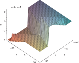
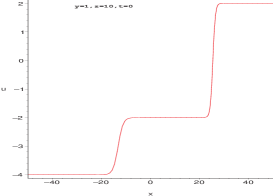
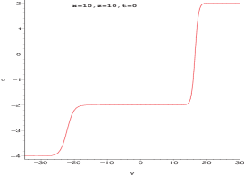
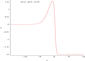
Figure 3.1: 1st 2-wave solution with $k_{1}=1,k_{2}=-2,m_{1}=1,m_{2}=5,c_{1}=1,c_{2}=2.$

    

    

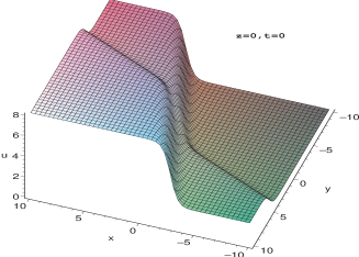
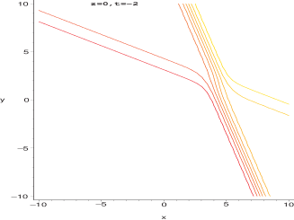
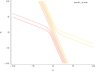
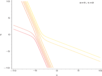
Figure 3.2: 2nd 2-wave solution with $k_{1}=1,k_{2}=3,l_{1}=2,l_{2}=1,c_{1}=1,c_{2}=2.$

Case 3 - Three-wave solutions:

Again similarly, we require the linear conditions:

$$\eta_{i,x}=k_{i}\eta_{i},\ \eta_{i,y}=l_{i}\eta_{i},\ \eta_{i,z}=m_{i}\eta_{i},\ \eta_{i,t}=-\omega_{i}\eta_{i},\ 1\leq i\leq 3,$$ (3.14)

where $k_{i},l_{i},m_{i},\omega_{i},\ 1\leq i\leq 3$, are constants, and thus, the solutions $\eta_{1},\eta_{2}$ and $\eta_{3}$ can be defined by

$$\eta_{i}=c_{i}e^{k_{i}x+l_{i}y+m_{i}z-\omega_{i}t},\ 1\leq i\leq 3.$$ (3.15)

where $c_{1},c_{2}$ and $c_{3}$ are arbitrary constants.

Let us now try the following particular pair of two polynomials of degree three:

$$\left\{\begin{array}[]{l}p(\eta_{1},\eta_{2},\eta_{3})=2[k_{1}\eta_{1}+k_{2}\eta_{2}+k_{3}\eta_{3}+a_{12}(k_{1}+k_{2})\eta_{1}\eta_{2}+a_{13}(k_{1}+k_{3})\eta_{1}\eta_{3}\vspace{2mm}\\ \qquad\qquad\qquad+a_{23}(k_{2}+k_{3})\eta_{2}\eta_{3}+a_{12}a_{13}a_{23}(k_{1}+k_{2}+k_{3})\eta_{1}\eta_{2}\eta_{3}],\vspace{2mm}\\ q(\eta_{1},\eta_{2},\eta_{3})=1+\eta_{1}+\eta_{2}+\eta_{3}+a_{12}\eta_{1}\eta_{2}+a_{13}\eta_{1}\eta_{3}+a_{23}\eta_{2}\eta_{3}+a_{12}a_{13}a_{23}\eta_{1}\eta_{2}\eta_{3},\end{array}\right.$$ (3.16)

where $a_{12}$, $a_{13}$ and $a_{23}$ are constants to determined. By the multiple exp-function method and using the differential relations in (3.14), we can have two solutions to the resulting algebraic system with Maple:

$$\omega_{i}=-\frac{3}{4}k_{i}-\frac{1}{4}{k_{i}}^{2}m_{i},\ 1\leq i\leq 3,$$ (3.17)

and

$$a_{ij}=\frac{(k_{i}-k_{j})^{2}}{(k_{i}+k_{j})^{2}},\ 1\leq i,j\leq 3,$$ (3.18)

when $l_{i}=k_{i},\ 1\leq i\leq 3$; and

$$\omega_{i}=-\frac{1}{4}{k_{i}}^{3}-\frac{3{l_{i}}^{2}}{4k_{i}},\ 1\leq i\leq 3,$$ (3.19)

and

$$a_{ij}={\frac{\left(k_{{i}}{k_{{j}}}^{2}-{k_{{i}}}^{2}k_{{j}}+k_{{i}}l_{{j}}-l_{{i}}k_{{j}}\right)\left(k_{{i}}{k_{{j}}}^{2}-{k_{{i}}}^{2}k_{{j}}-k_{{i}}l_{{j}}+l_{{i}}k_{{j}}\right)}{\left(k_{{i}}{k_{{j}}}^{2}+{k_{{i}}}^{2}k_{{j}}+k_{{i}}l_{{j}}-l_{{i}}k_{{j}}\right)\left(k_{{i}}{k_{{j}}}^{2}+{k_{{i}}}^{2}k_{{j}}-k_{{i}}l_{{j}}+l_{{i}}k_{{j}}\right)}},\ 1\leq i,j\leq 3,$$ (3.20)

when $m_{i}=k_{i},\ 1\leq i\leq 3$.

Then, the two corresponding 3-wave solutions are given by

$$u=u(x,y,z,t)=\frac{p(\eta_{1},\eta_{2},\eta_{3})}{q(\eta_{1},\eta_{2},\eta_{3})},$$ (3.21)

where $p$ and $q$ are defined by (3.16) and $\eta_{1},\eta_{2}$ and $\eta_{3}$ are defined by (3.15), either with the frequencies $\omega_{1},\omega_{2}$ and $\omega_{3}$ being given by (3.17) and $a_{12},\ a_{13}$ and $a_{23}$, by (3.18) when $l_{i}=k_{i},\ 1\leq i\leq 3$; or with the frequencies $\omega_{1},\omega_{2}$ and $\omega_{3}$ being given by (3.19) and $a_{12},\ a_{13}$ and $a_{23}$, by (3.20) when $m_{i}=k_{i},\ 1\leq i\leq 3$. All the unspecified involved constants in the solutions are arbitrary. Two specific solutions of those 3-wave solutions are plotted in the figures 3.3 and 3.4. In each figure, the first plot is three dimensional, and the other plots exploit the $x$-curves with $y=1$ and different $z$-values at different times or the contour plots with $z=0$ at different times.

   

   

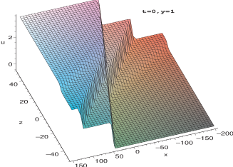
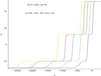
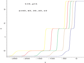
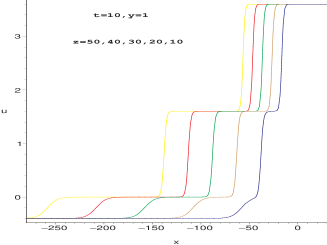
Figure 3.3: 1st 3-wave solution with $k_{1}=0.8,k_{2}=1.6,k_{3}=-0.6,l_{1}=-2,l_{2}=3,l_{3}=-1.5,c_{1}=0.9,c_{2}=0.8,c_{3}=1.2.$

    

    

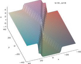
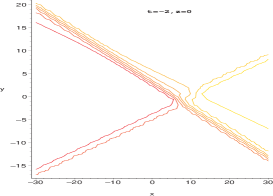
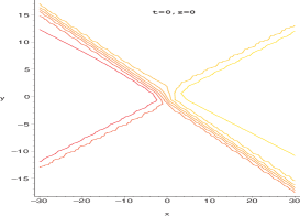
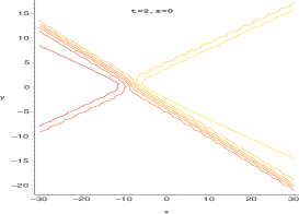
Figure 3.4: 2nd 3-wave solution with $k_{1}=0.8,k_{2}=1.6,k_{3}=-0.6,l_{1}=-2,l_{2}=3,l_{3}=-1.5,c_{1}=0.9,c_{2}=0.8,c_{3}=1.2.$

We emphasize that through the proposed multiple exp-function algorithm, two kinds of 2-wave solutions and 3-wave solutions are easily obtained for the potential-YTSF equation (1.1). If for 2-wave and 3-wave solutions, we take the general wave frequencies like (3.3), where $m_{1},k_{1},l_{1}$ have no relation, we will meet contradictions in the resulting algebraic systems. On the other hand, if the involved constants in (3.5) satisfy $b_{0}b_{1}<0$ and some of the constants $c_{i}$, $1\leq i\leq n$, in (3.13) and (3.21) are negative, the corresponding exact solutions become singular. Moreover, for the second case (i.e., $m_{i}=k_{i}$), even if the constants $c_{i}$ are positive in (3.13) and (3.21), the constants $a_{ij}$ can be negative, and thus, the solutions (3.13) and (3.21) can be singular. Taking special constants in our 1-wave, 2-wave and 3-wave solutions and considering equal angular wave numbers $l_{i}=m_{i}=k_{i}$ yields all special soliton solutions to the potential-YTSF equation (1.1), presented by Wazwaz in [43].

4 Concluding remarks

A direct and systematical solution procedure for constructing multiple wave solutions to nonlinear partial differential equations is proposed. The presented method is oriented towards ease of use and capability of computer algebra systems, allowing us to carry out the involved computation conveniently through powerful computer algebra systems. It is the use of computer algebra systems that in each case of 2-wave and 3-wave solutions, we are able to present two classes of concrete exact explicit solutions to the $3+1$ dimensional PYTSF equation, only in form of $u=f(t,x+y,z)$ or $u=f(t,x+z,y)$ (but not in a general form including $u=f(t,x,y+z)$). The key point of our approach is to search for rational solutions in a set of new variables defining individual waves. An application of our method yields specific 1-wave, 2-wave and 3-wave solutions to the $3+1$ dimensional PYTSF equation. The method can also be easily applied to other nonlinear evolution and wave equations in mathematical physics.

It is direct to check that the $3+1$ dimensional potential-YTSF equation (1.1) has the following class of polynomial solutions:

$$u_{1}=u_{1}(x,y,z,t)=a_{1}+a_{2}x+a_{3}y+a_{4}z+a_{5}t+a_{6}xy+a_{7}yz+a_{8}yt+a_{9}zt+a_{10}yzt,$$ (4.1)

where $a_{i},\ 1\leq i\leq 10$, are arbitrary constants. These are all polynomial solutions among a class of polynomial functions with $\deg(u_{1},x)=\deg(u_{1},y)=\deg(u_{1},z)=\deg(u_{1},t)=1$. On the other hand, there are other two solutions:

$$u_{2}=u_{2}(x,y,z,t)=a_{1}+a_{2}x+a_{3}y+a_{4}z+a_{5}t+f(z,t),$$ (4.2)

and

$$u_{3}=u_{3}(x,y,z,t)=a_{1}+a_{2}x+a_{3}z+a_{4}t+g(x)+h(t),$$ (4.3)

where $a_{i},\ 1\leq i\leq 5$, are arbitrary constants and $f,g,h$ are arbitrary functions in the indicated variables. Taking $f,g,h$ as polynomials engenders other polynomial solutions to the potential-YTSF equation (1.1), which can be of high degree. But the third one reduces to solutions to the $2+1$ dimensional potential Calogero-Bogoyavlenkii-Schiff equation, independent of the variable $y$.

It is our guess that higher-wave solutions to the $3+1$ dimensional potential-YTSF equation (1.1) could be presented in a parallel manner. But the required computation is pretty complicated, even in the case of 4-wave solutions. We hope that they could be presented and verified by some analytic way. Any general form of 2-waves and 3-waves, which does not involve any relation among the angular wave numbers $k_{i},l_{i},m_{i}$, will be more interesting and important.

References

- [1] H. B. Lan, K. L. Wang, Exact solutions for two nonlinear equations: I., J. Phys. A: Math. Gen. 23 (1990) 3923–3928.
- [2] W. Malfliet, Solitary wave solutions of nonlinear wave equations, Amer. J. Phys. 60 (1992) 650–654.
- [3] E. J. Parkes, B. R. Duffy, An automated tanh-function method for finding solitary wave solutions to non-linear evolution equations. Comput. Phys. Commun. 98 (1996) 288–300.
- [4] W. X. Ma, Travelling wave solutions to a seventh order generalized KdV equation, Phys. Lett. A 180 (1993) 221–224.
- [5] B. R. Duffy, E. J. Parkes, Travelling solitary wave solutions to a seventh-order generalized KdV equation, Phys. Lett. A 214 (1996) 271–272.
- [6] W. X. Ma, D. T. Zhou, Explicit exact solutions to a generalized KdV equation, Acta Mathematica Scientia 17(Supp.) (1997) 168–74.
- [7] M. L. Wang, Solitary wave solutions for variant Boussinesq equations, Phys. Lett. A 199 (1995) 169–72.
- [8] E. G. Fan, A note on the homogenous balance method, Phys. Lett. A 246 (1998) 403–406.
- [9] W. X. Ma, B. Fuchssteiner, Explicit and exact solutions to a Kolmogorov-Petrovskii-Piskunov equation, Internat. J. Non-Linear Mech. 31 (1996) 329–338.
- [10] E. G. Fan, Extended tanh-function method and its applications to nonliear equations, Phys. Lett. A 277 (2000) 212–218.
- [11] T. W. Han, X. L. Zhuo, Rational form solitary wave solutions for some types of high order nonlinear evolution equations, Ann. Differential Equations 16 (2000) 315–319.
- [12] C. T. Yan, A simple transformation for nonlinear waves, Phys. Lett. A 224 (1996) 77–84.
- [13] A. M. Wazwaz, A sine-cosine method for handling nonlinear wave equations, Math. Comput. Modelling 40 (2004) 499–508.
- [14] A. M. Wazwaz, The tanh-coth method for solitons and kink solutions for nonlinear parabolic equations, Appl. Math. Comput. 188 (2007) 1467–1475.
- [15] J. H. He, H. X. Wu, Exp-function method for nonlinear wave equations, Chaos, Solitons and Fractals 30 (2006) 700–708.
- [16] J. H. He, M. A. Abdou, New periodic solutions for nonlinear evolution equations using Exp-function method, Chaos, Solitons and Fractals 34 (2007) 1421–1429.
- [17] W. X. Ma, J. H. Lee, A transformed rational function method and exact solutions to the dimensional Jimbo-Miwa equation, Chaos, Solitons and Fractals 42 (2009) 1356 -1363.
- [18] R. Hirota, The Direct Method in Soliton Theory, Cambridge Tracts in Mathematics 155 (Cambridge University Press, Cambridge, 2004).
- [19] Y. Zhang, L. Y. Ye, Y. N. Lv, H. G. Zhao, Periodic wave solutions of the Boussinesq equation, J. Phys. A: Math. Gen. 40 (2007) 5539–5549.
- [20] W. X. Ma, R. G. Zhou, L. Gao, Exact one-periodic and two-periodic wave solutions to Hirota bilinear equations in dimensions, Modern Phys. Lett. A 24 (2009) 1677–1688.
- [21] S. J. Yu, K. Toda, N. Sasa, T. Fukuyama, -soliton solutions to the Bogoyavlenskii-Schiff equation and a quest for the soliton solution in dimensions, J. Phys. A: Math. Gen. 31 (1998) 3337–3347.
- [22] M. S. Bruzón, M. L. Gandarias, S. Muriel, Kh. Ramíres, S. Saez, F. R. Romero, The Calogero-Bogoyavlenskii-Schiff equation in dimension , Teoret. Mat. Fiz. 137 (2003) 14–26; Theoret. Math. Phys. 137 (2003) 1367–1377.
- [23] F. Calogero, A. Degasperis, Nonlinear evolution equations solvable by the inverse spectral transform I, Nuovo Cimento B 32 (1976) 201–242.
- [24] Z. Y. Yan, New families of nontravelling wave solutions to a new -dimensional potential-YTSF equation, Phys. Lett. A 318 (2003) 78–83.
- [25] C. L. Bai, H. Zhao, Generalized extended tanh-function method and its application, Chaos, Solitons and Fractals 27 (2006) 1026–1035.
- [26] T. X. Zhang, H. N. Xuan, D. F. Zhang, C. J. Wang, Non-travelling wave solutions to a -dimensional potential-YTSF equation and a simplified model for reacting mixtures, Chaos, Solitons and Fractals 34 (2007) 1006–1013.
- [27] L. N. Song, H. Q. Zhang, A new variable coefficient Korteweg-de Vries equation-based sub-equation method and its application to the -dimensional potential-YTSF equation, Appl. Math. Comput. 189 (2007) 560–566.
- [28] S. Y. Lou, J. Z. Lu, Special solutions from the variable separation approach: the Davey-Stewartson equation, J. Phys. A: Math. Gen. 29 (1996) 4209–4215.
- [29] N. A. Kudryashov, Seven common errors in finding exact solutions of nonlinear differential equations, Commun. Nonlinear Sci. Numer. Simul. 14 (2009) 3507–3529.
- [30] W. X. Ma, H. Y. Wu, J. S. He, Partial differential equations possessing Frobenius integrable decompositions, Phys. Lett. A 364 (2007) 29–32.
- [31] W. X. Ma, An exact solution to two-dimensional Korteweg-de Vries-Burgers equation, J. Phys. A: Math. Gen. 26 (1993) L17–L20.
- [32] S. K. Liu, Z. T. Fu, S. D. Liu, Q. Zhao, Jacobi elliptic function expansion method and periodic wave solutions of nonlinear wave equations, Phys. Lett. A 289 (2001) 69–74.
- [33] E. J. Parkes, B. R. Duffy, P. C. Abbott, The Jacobi elliptic-function method for finding periodic-wave solutions to nonlinear evolution equations, Phys. Lett. A 295 (2002) 280–286.
- [34] Y. Z. Peng, A Mapping Method for Obtaining Exact Travelling Wave Solutions to Nonlinear Evolution Equations, Chinese J. Phys. 41 (2003) 103–110.
- [35] E. Yomba, On exact solutions of the coupled Klein-Gordon-Schrodinger and the complex coupled KdV equations using mapping method, Chaos, Solitons and Fractals 21 (2004) 209–229.
- [36] Y. Zhou, M. L. Wang, Y. M. Wang, Periodic wave solutions to a coupled KdV equations with variable coefficients, Phys. Lett. A 308 (2003) 31–36.
- [37] J. B. Liu, K. Q. Yang, The extended -expansion method and exact solutions of nonlinear PDEs, Chaos, Solitons and Fractals 22 (2004) 111–121.
- [38] Y. Chen, Z. Y. Yan, New exact solutions of -dimensional Gardner equation via the new sine-Gordon equation expansion method, Chaos, Solitons and Fractals 26 (2005) 399–406.
- [39] M. L. Wang, X. Z. Li, J. L. Zhang, The -expansion method and travelling wave solutions of nonlinear evolution equations in mathematical physics. Phys. Lett. A 372 (2008) 417–423.
- [40] A. Boz, A. Bekir, Application of Exp-function method for -dimensional nonlinear evolution equations, Comput. Math. Appl. 56 (2008) 1451–1456.
- [41] Y. P. Wang, Solving the (3+1)-dimensional potentail-YTSF equation with exp-function method, J. Phys. A: Conf. Series 96 (2008) 012186, pp.7.
- [42] X. P. Zeng, Z. D. Dai, D. L. Li, New periodic soliton solutions for the (3+1)-dimensional potential-YTSF equation, Chaos, Solitons and Fractals 42 (2009) 657–661.
- [43] A. M. Wazwaz, Multiple-soliton solutions for the Calogero-Bogoyavlenskii-Schiff, Jimbo-Miwa and YTSF equations, Appl. Math. Comput. 203 (2008) 592–597.