An Energy Conserving Parallel Hybrid Plasma Solver

Abstract

We investigate the performance of a hybrid plasma solver on the test problem of an ion beam. The parallel solver is based on cell centered finite differences in space, and a predictor–corrector leapfrog scheme in time. The implementation is done in the FLASH software framework. It is shown that the solver conserves energy well over time, and that the parallelization is efficient (it exhibits weak scaling).

1 Introduction

Modeling of collisionless plasmas are often done using fluid magnetohydrodynamic models (MHD). The MHD fluid approximation is however questionable when the gyro radius of the ions are large compared to the spatial region that is studied. On the other hand, kinetic models that discretize the full velocity space, or full particle in cell (PIC) models that treat ions and electrons as particles, are very computational expensive. For problems where the ion time- and spatial scales are of interest, hybrid models provide a compromise. In such models, the ions are treated as discrete particles, while the electrons are treated as a (often massless) fluid. This mean that the electron time- and spatial scales do not need to be resolved, and enables applications such as modeling of the solar wind interaction with planets. For a detailed discussion of different models, see Ledvina et al. (2008).

Here we present an finite difference implementation of a hybrid model in the FLASH parallel computational framework, along with test cases that show that the implementation scales well and conserve energy well.

2 The hybrid equations

In the hybrid approximation, ions are treated as particles, and electrons as a massless fluid. In what follows we use SI units. The trajectory of an ion, $\mathbf{r}(t)$ and $\mathbf{v}(t)$, with charge $q$ and mass $m$, is computed from the Lorentz force,

$$\frac{\displaystyle d\mathbf{r}}{\displaystyle dt}=\mathbf{v},\quad\frac{\displaystyle d\mathbf{v}}{\displaystyle dt}=\frac{\displaystyle q}{\displaystyle m}\left(\mathbf{E}+\mathbf{v}\times\mathbf{B}\right),$$

where $\mathbf{E}=\mathbf{E}(\mathbf{r},t)$ is the electric field, and $\mathbf{B}=\mathbf{B}(\mathbf{r},t)$ is the magnetic field. The electric field is given by

$$\mathbf{E}=\frac{\displaystyle 1}{\displaystyle\rho_{I}}\left(-\mathbf{J}_{I}\times\mathbf{B}+\mu_{0}^{-1}\left(\nabla\times\mathbf{B}\right)\times\mathbf{B}\right)-\nabla p_{e},$$

where $\rho_{I}$ is the ion charge density, $\mathbf{J}_{I}$ is the ion current, $p_{e}$ is the electron pressure, and $\mu_{0}=4\pi\cdot 10^{-7}$ is the magnetic constant. Then Faraday’s law is used to advance the magnetic field in time,

$$\frac{\displaystyle\partial\mathbf{B}}{\displaystyle\partial t}=-\nabla\times\mathbf{E}.$$

3 A cell centered finite difference hybrid solver

We use a cell-centered representation of the magnetic field on a uniform grid. All spatial derivatives are discretized using standard second order stencils. Time advancement is done by a predictor-corrector leapfrog method with subcycling of the field update, denoted cyclic leapfrog (CL) by Matthews (1994). An advantage of the discretization is that the divergence of the magnetic field is zero, down to round off errors. The ion macroparticles (each representing a large number of real particles) are deposited on the grid by a cloud-in-cell method (linear weighting), and interpolation of the fields to the particle positions are done by the corresponding linear interpolation. Initial particle positions are drawn from a uniform distribution, and initial particle velocities from a Maxwellian distribution. Further details of the algorithm can be found in Holmström (2011).

4 Implementing the solver in FLASH

We use an existing software framework, FLASH, developed at the University of Chicago (Fryxell et al., 2000), that implements a block-structured adaptive (or uniform) Cartesian grid and is parallelized using the Message-Passing Interface (MPI) library for communication. It is written in Fortran 90, well structured into modules, and open source. Output is handled by the HDF5 library, providing parallel I/O. Although the FLASH framework has mostly been used for fluid modeling, it has support for particles which we have used to implement a hybrid solver using the latest version of the framework, FLASH3.

The advantage of using an existing framework when implementing a solver is that all grid operations, parallelization and file handling is done by standard software calls that have been well-tested. Also, there is an existing infrastructure for parameter files and setup directories that simplifies code handling. The concept of a setup directory is that one can place modified versions of any routine in the directory, and this new version will be used during the build process. This is an easy way to handle different versions of code for different runs of the solver.

In particular, many of the basic operations needed for a PIC code are provided as standard operations in FLASH:

• Deposit charges onto the grid: call Grid_mapParticlesToMesh()

• Interpolate fields to particle positions: call Grid_mapMeshToParticles()

• Ghost cell update for all blocks: call Grid_fillGuardCells()

The advantage of a parallel solver is the ability to handle larger computational problems than on a single processor, both in terms of computational time and memory requirements. This is especially important for PIC solvers which are computational intensive compared to fluid solvers. Since we typically have 10–100 particles per cell, the computational work will be dominated by operations on the particles: moving the particles and grid-particle operations.

That a code works well in parallel is usually investigated by looking at how the code scales. For the case of strong scaling, a fixed size problem is run on different numbers of processors. Ideally the execution time should decrease proportional to the number of processors (linear scaling). This is however difficult to achieve in real world applications. Sequential parts of the program quickly dominate the execution time. An alternative concept is that of weak scaling. Here the problem size is increased at the same time as we add more processors. That this implementation of a hybrid solver exhibits weak scaling is shown in Fig. 1. For this application, weak scaling is adequate, since we aim to solve larger problems using a constant wall clock time.

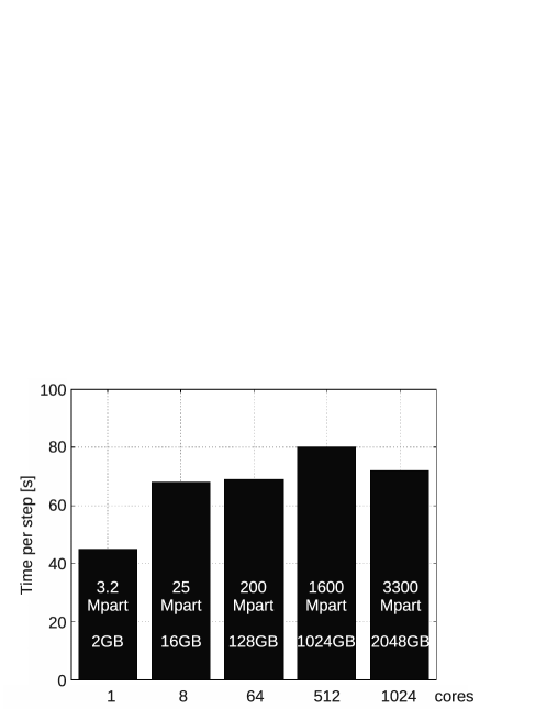
Figure 1: Timings for the hybrid solver, illustrating that the code scales well for large problems. We see that the wall clock time required for a time step for this particular test is roughly constant around 70 seconds independent of problem size. Total number of particles, and total available memory is shown on each bar. All runs were done on the Akka cluster at the High Performance Computing Center North (HPC2N) at Umeå University, Sweden. A 672 node cluster with an Infiniband interconnect, where each cluster node has two quad core Intel Xeon processors and 16 GB of RAM.

5 Accuracy of the solver

It is not easy to check the correctness and accuracy of a hybrid solver. There are not many non-trivial test problems that have analytical solutions to compare with. One can of course check the results against published results but that only gives a crude sanity check of the code. One option is to investigate the conservation of total energy. This is a crucial quantity since the behavior of a plasma is a constant exchange of energy between the kinetic energy of the particles and the energy stored in the electromagnetic fields. It is also a quantity that easily can be measured for any simulation, especially if the boundary conditions are periodic. We therefore choose to perform numerical experiments with an ion beam, a test problem that strongly exhibits this exchange of energy between particles and fields, to study the conservation of total energy.

5.1 One-dimensional ion beam

A classic plasma model problem is that of an ion beam into a plasma (Winske & Leroy, 1984; Winske, 1985; Winske & Quest, 1986). Matthews (1994) describes a two-dimensional simulation of a low density ion beam through a background plasma. The initial condition has a uniform magnetic field, with a beam of ions, number density $n_{b}$, propagating along the field with velocity $v_{b}=10v_{A}$, where $v_{A}=B/\sqrt{\mu_{0}nm_{i}}$ is the Alfvén velocity, through a background (core) plasma of number density $n_{c}$. Both the background and beam ions have thermal velocities $v_{th}=v_{A}$. Here we study what is denoted a resonant beam with $n_{b}=0.015\,n_{c}$ and $v_{c}=-0.2\,v_{A}$. Electron temperature is assumed to be zero, so the electron pressure term in the electric field equation of state is zero. The weight of the macroparticles are chosen such that there is an equal number of core and beam macroparticles, each beam macroparticles thus represent fewer real ions than the core macroparticles. The number of magnetic field update subcycles is nine.

The spatial extent of the domain is 22016 km along the $x$-axis, divided up in 256 cells with periodic boundary conditions. The core number density is $n_{c}=7$ cm^-3. The magnetic field magnitude is $B=6$ nT directed along the $x$-axis, which give an Alfvén velocity of 50 km/s and an ion inertial length of $\delta_{i}$=86 km, where $\delta_{i}=v_{A}/\Omega_{i}$ and $\Omega_{i}=q_{i}B/m_{i}$ is the ion gyrofrequency. The time step is 0.0865 s = $0.05\,\Omega_{i}^{-1}$, and the cell size is $\delta_{i}$. The number of particles per cell is 32. In Fig. 2 we show a velocity space plot of the macro-ions at time $t=34.6$ s $\approx 20\,\Omega_{i}^{-1}$. This can be compared to Fig. 5 in Winske & Leroy (1984).

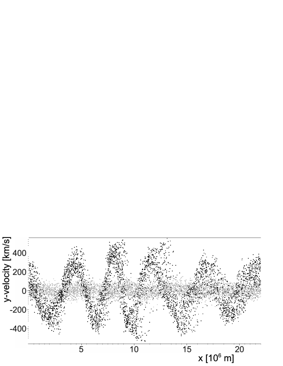
Figure 2: Velocity space plot for a one-dimensional ion beam. Velocity along the $y$-axis as a function of position at time $t=34.6$ s $\approx 20\,\Omega_{i}^{-1}$. Each gray dot is a core macro-ion, and each black dot is a beam macro-ion.

The kinetic energy of the ions, the energy stored in the electromagnetic fields, and total energy, as a function of time, are shown in Fig. 3. The magnetic and electric field energies are computed as

$$\frac{1}{2\mu_{0}}\int\left|\mathbf{B}\right|^{2}dV,\quad\mbox{ and }\quad\frac{\epsilon_{0}}{2}\int\left|\mathbf{E}\right|^{2}dV,$$

respectively. Here $\epsilon_{0}$ is the vacuum permittivity, $\epsilon_{0}\mu_{0}c^{2}=1$. Note that the electric field energy is too small to be visible in the figure (orders of magnitude smaller than the magnetic field energy).

Figure 3: Energy partition for a one-dimensional ion beam as a function of time.

At $t=86$ s $\approx 50\,\Omega_{i}^{-1}$ the relative energy error is less than 0.1%. This can be compared to the error of 11% given by Matthews (1994).

5.2 Two-dimensional ion beam

In the two-dimensional case we have a square grid with sides of length 22016 km, and 128 cells in each direction with periodic boundary conditions. The time step is 0.0216 s = $0.05\,\Omega_{i}^{-1}$, and the cell widths are $2\delta_{i}$. The number of particles per cell is 16. Otherwise the setup is identical to the one-dimensional case. In Fig. 4 we show the magnitude of the magnetic field $y$-component at time $t=77.85$ s $\approx 46\,\Omega_{i}^{-1}$. This can be compared to Fig. 5 in Winske & Quest (1986).

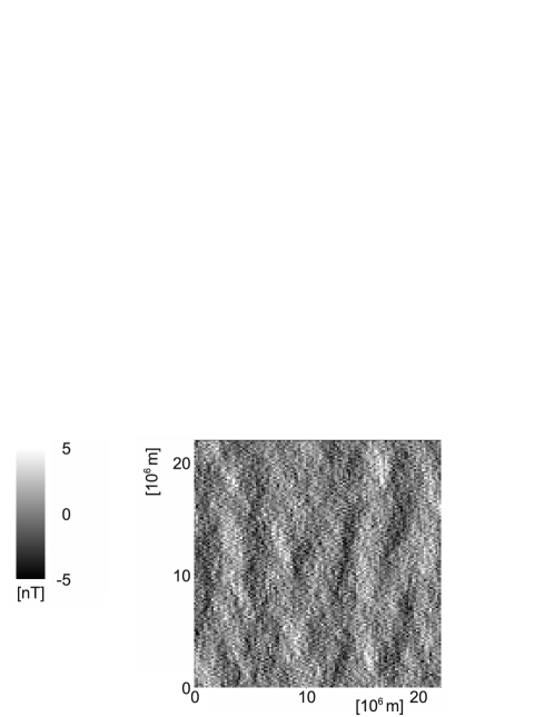
Figure 4: The magnetic field $y$-component for a two-dimensional ion beam at time $t=77.85$ s $\approx 46\,\Omega_{i}^{-1}$.

The kinetic energy of the ions, the energy stored in the electromagnetic fields, and total energy, as a function of time, are shown in Fig. 5.

Figure 5: Energy partition for a two-dimensional ion beam as a function of time.

We can note that the fluctuations in magnetic and kinetic energy is smaller than in the one-dimensional case, consistent with the observations by Winske & Quest (1986). The total relative energy gain at $t=173$ s $\approx 100\,\Omega_{i}^{-1}$ is less than 0.004%. This can be compared to Winske & Quest (1986), where the stated energy gain was less than 2% and smoothing of the fields was needed for numerical stability.

6 Summary and conclusions

We have investigated the performance of a hybrid solver on the classical test case of an ion beam, in one and two dimensions. It is shown that the cell centered finite difference solver conserves energy very well. The change in total energy over time is more than an order of magnitude smaller than for two previously published solvers. Also, the solver is numerically stable over long times without any smoothing of the fields. It is planned that this hybrid solver will be part of a future release of the FLASH code.

Acknowledgments

This research was conducted using resources provided by the Swedish National Infrastructure for Computing (SNIC) at the High Performance Computing Center North (HPC2N), Umeå University, Sweden. The software used in this work was in part developed by the DOE-supported ASC / Alliance Center for Astrophysical Thermonuclear Flashes at the University of Chicago.

References

- Fryxell et al. (2000) Fryxell, B., et al. 2000, The Astrophysical Journal Supplement Series, 131, 273
- Holmström (2011) Holmström, M. 2011, in Proceedings of ENUMATH 2009 (Springer), 451. ArXiv:0911.4435v2
- Ledvina et al. (2008) Ledvina, S., Ma, Y.-J., & Kallio, E. 2008, Space Sci. Rev., 143
- Matthews (1994) Matthews, A. P. 1994, Journal of Computational Physics, 112, 102
- Winske (1985) Winske, D. 1985, Space Science Reviews, 42, 53
- Winske & Leroy (1984) Winske, D., & Leroy, M. M. 1984, Journal of Geophysical Research, 89, 2673
- Winske & Quest (1986) Winske, D., & Quest, K. 1986, Journal of Geophysical Research, 91, 8789