First-principles approach to rotational-vibrational frequencies and infrared intensity for H₂ adsorbed in nanoporous materials

Abstract

The absorption sites and the low-lying rotational and vibrational (RV) energy states for H₂ adsorbed within a metal-organic framework are calculated via van der Waals density functional theory. The induced dipole due to bond stretching is found to be accurately given by a first-principles driven approximation using maximally-localized-Wannier-function analysis. The strengths and positions of lines in the complex spectra of RV transitions are in reasonable agreement with experiment, and in particular explain the experimentally mysteriously missing primary line for para hydrogen.

Gas adsorption into nanoporous materials is of great interest for both fundamental science and applications. Molecular H₂ is challenging because it can vibrate, rotate, and translate quantum mechanically about its binding site due to its small mass. The vibration-rotation (RV) excitations induced by infrared (IR) absorption thus provide rich information Chabal . However, determining the origin and strength of these lines is challenging because large unit cells are encountered in typical nanoporous structures, and the dynamic dipole is distributed over spatially remote parts of the structure. To determine the absorption intensity, a precisely tractable experimental quantity, one must not only calculate the dipole, but also evaluate the quantum mechanical matrix element. An effective approximation scheme for doing this has not hitherto been found.

Here, we present such a scheme based on the combination of a self-consistent van der Waals density functional (vdW-DF) approach vdw with maximally-localized-Wannier-function (MLWF) analysis wannier ; Marzari and apply it to H₂ adsorption in a prototypical metal-organic framework, MOF-5 Yaghi2003 . Such materials have been extensively explored for hydrogen storage Murray , gas separation, catalysis, and sensors Czaja . We analyze the dynamical properties of the adsorbed H₂, finding results consistent with experiment. Importantly, we apply the MLWF analysis to calculate the induced dipole moment due to H₂ adsorption and bond stretching, decomposing the dipole into the contributions from both adsorbed dihydrogen and MOF. Monitoring the change in each Wannier center of the MOF structure upon H₂ adsorption provides an intuitive picture by breaking the H₂-sorbent interaction into individual components of the MOF structure, thus identifying the parts that directly interact with the dihydrogen. Such knowledge is important to optimize MOF structures for desired properties. In the present case, we use this information to calculate the dynamical dipole moment and its matrix element for H₂ vibrational transitions and RV transitions. We find that the IR intensity of the purely vibrational mode for para hydrogen is only about 2.5% of that for ortho hydrogen at the primary adsorption site, which agrees beautifully with the missing line in the experiment. FitzGerald2008 . A selection rule for RV transitions at the relevant site is also obtained and supported by the IR data.

The H₂ binding sites are efficiently determined by self-consistent vdW-DF calculations vdw . A series of total energy calculations for different bond lengths, orientations, and center-of-mass positions respectively are performed keeping the MOF atoms fixed at experimental positions Rowsell2005 . The resulting potential energy surfaces are then used in the corresponding radial and rigid rotor Schrödinger equations respectively to extract the vibrational, rotational and translational frequencies Kongprb ; Kongprl . Anharmonic effects are fully included.

It has been shown that the sum of the Wannier-function centers is connected to the Berry phase theory of bulk polarization wannier . The dipole in the unit cell is given by $\mathbf{u}=e\sum_{m}Z_{m}\mathbf{R}_{m}-e\sum_{n,spin}\mathbf{r}_{n}$, where $Z_{m}$ and $\mathbf{R}_{m}$ are the atomic number and position of the $m^{\mathrm{th}}$ nuclei and $\mathbf{r}_{n}$ is the center of the $n^{\mathrm{th}}$ Wannier function. Importantly, it is trivial to decompose the total dipole into components in various parts of the structure Marzari , which goes beyond the Berry-phase method. Thereby, we may use the change of Wannier center upon adsorption as a qualitative measure for understanding the H₂-MOF interaction and to determine the important parts of the MOF that directly interact with hydrogen.

There are four types of adsorption sites in this structure, as established experimentally Yildirim2005 and theoretically Sillar2009 , with reasonable agreement. We start with the positions determined by neutron scattering Yildirim2005 and relax the H₂ with the vdW-DF approach, thereby confirming the positions of the four sites, named the cup, O3, O2, and benzene sites Yildirim2005 . Fig. 1 shows the position of the cup site and a portion of the MOF-5 structure where there exists 3-fold rotation symmetry among the three benzene ring branches. The distance between the H₂ center-of-mass position and the oxygen atom passing through the rotation axis is about 4.2Å  which is somewhat larger than the measured value of 3.8Å Yildirim2005 due to a known vdW-DF overestimation of bond lengths Langreth2009 . Fig. 1 also shows the shift of the Wannier centers upon H₂ adsorption with respect to the bare MOF and the free H₂. See Supplemental Material for other sites . These figures show that the Wannier centers associated with the $\pi$ bonds in the benzene ring change significantly upon H₂ adsorption for all four adsorption sites, showing a clear and intuitive picture of the MOF components that interact directly with the adsorbed H₂.

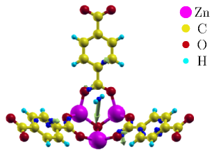
Figure 1: The primary adsorption site and the change of Wannier centers (blue balls) due to H₂ adsorption compared to bare MOF and free H₂. Vector lengths are enlarged by 1200. The structure shown is just a fraction of the unit cell.

Table 1 shows both the theoretical and experimental stretch frequency shifts of the adsorbed H₂ with respect to the corresponding free H₂ value. The agreement is good, within a reasonable error. Importantly, the origin of the IR peaks at $-$19 and $-$17 cm^-1 (not understood in the experiment FitzGerald2008 ) is now unraveled with the aid of our calculational results. Note that the calculated binding energies at O2 and O3 sites are very close. However, vdW-DF typically overestimates intermediate-range interactions Lee . Since O3 has three benzene neighbors while O2 has two, the overestimation for the O3 site is expected to be larger than that for the O2 site. As a result, the O2 site is probably more favorable energetically and should get populated more than the O3 site. This is consistent with the measurements where the $-$17 cm^-1 peak is quite weak and appears only as a shoulder to the main line at $-$19 cm^-1. We therefore assign the $-$19 cm^-1 peak to the O2 site whereas $-$17 cm^-1 to O3.

Table 1: Theory vs experiment FitzGerald2008 for the stretch frequency shift of the adsorbed H₂ relative to free H₂. See text for zero point energies (not included in the binding energies E_B here).

site	Theory	Expr.	Calculated EB
	(cm-1)	(cm-1)	(kJ/mol)
cup	$-$23	$-$27.5	$-$11.1
O2	$-$22	$-$19.0	$-$7.9
O3	$-$13	$-$17	$-$7.8
benzene	$-$15	—	$-$5.4

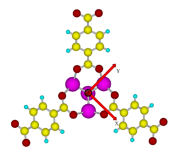
Figure S2: Illustration of the MOF frame of reference. Origin is at the cup adsorption sites and Z is along the <111>direction of cubic crystal lattice shown in Fig. S1. It is also the 3-fold rotation axis.

The IR spectra also show some RV lines where both vibrational and rotational states change during a single transition. Usually inelastic neutron scattering is employed to study the H₂ rotational states and has been already applied to H₂ in MOF-5 Yaghi2003 ; Rowselljacs2005 . However, the low energy resolution limits detailed analysis. We therefore consider the RV measured with IR  FitzGerald2008 for comparison with our rotational calculations. The left panel of Fig. 2 is the angular potential energy surface at the cup site. The coordinate system is chosen so that the origin is at the cup site and the $Z$ axis is the 3-fold rotation axis (see Fig. S2 in Supplemental Material ). Fig. 2 shows that H₂ tends to lie in the $XY$ plane and to be perpendicular to the rotation axis ($Z$). The energies for in-plane orientations are almost uniform. Therefore, the rotation is essentially two dimensional, as shown by the flattened ground-state angular wave function in the right panel of Fig. 2. Combining the stretch frequency and the rotational energies (see Supplemental Material), we obtain the RV frequencies. The results for the cup site are shown as S transitions in Table 2, where the frequency shifts are listed relative to the corresponding free H₂ values (see Supplemental Material for other sites). The magnitude of the shifts is consistent between theory and experiment, particularly for the leading peaks in each category that are most intense.

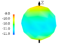
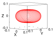
Figure 2: left: Orientational dependence of the binding energy (kJ/mol) at the cup site; right: Ground state $|\psi_{rot}|^{2}$. The distance from the origin is the probability for that orientation.

We also calculated the translational frequencies at the cup site associated with the motion of the whole H₂ against the adsorption site. The three translational frequencies, at 95, 108 and 133 cm^-1 respectively, are consistent with the value of 84 cm^-1 extracted from IR spectra FitzGerald2008 . They are also similar to that observed for H₂ in C₆₀ (110 cm^-1) FitzGerald2002 . The determination of the rotational and translational states gives the corresponding zero point energies of $\sim$0.5 and 2 kJ/mol for H₂ at the cup site. The binding energy after corrections is therefore about 8.5 kJ/mol and somewhat larger than the measured adsorption enthalpy of $\sim$5 kJ/mol Rowsell2006 ; Kaye2005 . This overestimation by vdW-DF, also found in other MOF materials Kongprb , is attributed to overestimation of the intermediate-range interactions Lee .

The measured IR spectra for the cup adsorption site shows a strong pure vibrational peak due to the ortho-H₂, while the corresponding para line is not observed. Since the orientational energy map only shows a small rotational barrier, the missing para-H₂ line cannot be explained by the assumption of a frozen H₂ orientation. Moreover, the local structure around this site has $C_{3v}$ symmetry. The rotational state of the para H₂ has the same symmetry as $Z$ and transforms as $A1$. Therefore the transitions between two $A1$ states should be IR active, even though the X and Y components of the dipole give a vanishing contribution by symmetry.

To understand the unexpected missing para-H₂ line and to calculate the line weights in the more complex RV spectra, we evaluate the transition dipole integral explicitly. Assuming the electronic state remains in the ground state and the RV wave function is separable, one has $I_{\alpha}=\langle\psi_{vib}^{f}\psi_{rot}^{f}|u_{\alpha}|\psi_{vib}^{i}\psi_{rot}^{i}\rangle$, where $u$ is the dipole moment and $\alpha=X,Y$, or $Z$; the translational motion associated with H₂ center-of-mass is not included. The dipole is a function of the H₂ internuclear distance, $R$, and the bond orientation is defined by $(\theta,\phi)$. It can be expanded as $u_{\alpha}(R,\theta,\phi)=u_{\alpha}(R_{0},\theta,\phi)+\left.u_{\alpha}^{\prime}(R,\theta,\phi)\right|_{R_{0}}\Delta R$ where $R_{0}$ is the equilibrium bond length, and $u_{\alpha}^{\prime}$ is the derivative of $u_{\alpha}$ with respect to $R$. Since the vibrational wave functions depend only on the inter-nuclear distance, the integral of the first term vanishes for transitions between different vibrational states due to orthogonality. We find $I_{\alpha}=\langle\psi_{vib}^{f}|\Delta R|\psi_{vib}^{i}\rangle\langle\psi_{rot}^{f}|u_{\alpha}^{\prime}(R_{0},\theta,\phi)|\psi_{rot}^{i}\rangle$, where $|\psi_{rot}^{i}\rangle\equiv|j_{i}m_{i}\rangle$ with $j$ even (odd) for para (ortho) H₂, and similarly for $|\psi_{rot}^{f}\rangle$. The radial integral is a constant for both ortho and para H₂ and therefore unnecessary for understanding the missing line of para-H₂. The angular integral determines the relative intensity between them. We now need to evaluate this integral, for which $u_{\alpha}^{\prime}(R_{0},\theta,\phi)$ remains to be calculated.

To perform ab initio calculations for $u_{\alpha}^{\prime}$ for every ($\theta$,$\phi$) is computationally expensive and impractical for this system. A possible approach is to compute the dipole from first principles for a few H₂ orientations and derive from them the dipole of all the other orientations. This becomes feasible if one can write the dipole as

$$u_{\alpha}=\sum_{i}C_{i,\alpha}F_{i,\alpha}(\theta,\phi)$$ (1)

where $F$ are some known functions and the summation needs to be run over only a few terms. This approach is appropriate if one realizes that H₂ and MOF are weakly interacting and the dipole induced on each other can be well described within a classical picture. First, MOF atoms produce an electric field ($\vec{E}$) which induces a dipole on H₂. At the cup site, the field is along Z due to the rotational symmetry so it can be easily shown that the induced dipole on H₂ is of the form in Eq. (1) by projecting the field perpendicular and parallel to the H₂ bond and calculating the corresponding dipole components. A second contribution to the total dipole of the system arises from the H₂ permanent quadrupole inducing a dipole on the MOF. The quadrupolar potential and the corresponding electric field at position $\mathbf{r}$, depend on $\mathbf{r}$, the H₂ quadrupole and the bond orientation, which are again of the form in Eq. (1). This field shifts the MOF charge density and induces a dipole. The total dipole on the MOF may be formally calculated by multiplying the electric field by the polarizability at the same position and integrating over the whole MOF. This procedure extends the classical picture of point charge into the continuous charge density regime. It cannot be performed in practice since the polarizability is not available. However, the final result for the dipole would be like the expression in Eq. (1), since the integration runs over the MOF space while ($\theta,\phi$) would be left unchanged. One can similarly add second-order corrections where the induced dipole on H₂ and MOF further produce dipole on each other. The final equation after this correction turns out to be quite simple for cup site absorption (see the Supplemental Material for derivation) and reads

$$u^{s}_{X} =C_{1}^{s}\sin 2\theta\cos\phi-(C_{2}^{s}\cos 2\phi-C_{3}^{s}\sin 2\phi)\sin^{2}\theta$$

$$u^{s}_{Y} =C_{1}^{s}\sin 2\theta\sin\phi+(C_{2}^{s}\sin 2\phi+C_{3}^{s}\cos 2\phi)\sin^{2}\theta$$ (2)

$$u^{s}_{Z} =C_{4}^{s}\cos^{2}\theta+C_{5}^{s},$$

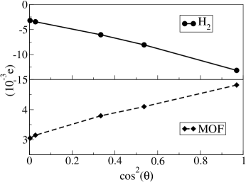
Figure S7: $\partial{u_{Z}}/\partial{R}$ vs $\cos^{2}\theta$ for the induced dipole on H₂ and MOF. $u^{\prime}_{Z}$ was calculated as the difference between the dipole moments at equilibrium bond length and a stretch of 0.05Å.

where $s$ could be H₂, MOF, or the total system. The C coefficients depend on the H₂ quadrupole, polarizability and MOF geometry which are kept fixed during the vibrational transition. From Eq. (2) we see that only two orientations (each orientation gives three equations) are required to determine the five constants and correspondingly the dipole for any other orientations. To test this model, we calculate $u^{\prime}_{Z}$ for several H₂ orientations. Good linearity is obtained between $u^{\prime}_{Z}$ and $\cos^{2}\theta$ (see Fig. S7 in Supplemental Material), in agreement with our model. X and Y components are also consistent with our model (see Supplemental Material).

Table 2: Theory vs. experiment FitzGerald2008 for RV transitions at the cup site. The frequency shift $\Delta$v (cm^-1) is relative to the corresponding free H₂ value. The theoretical intensity [$\propto I_{\alpha}^{2}$ times the 30K Boltzmann factor (times 3 for ortho)] is normalized to 100 for the strongest line; strong (str), weak (wk), and absent (abs) describe the experimental intensity.

	$m_{i}$	$m_{f}$	Theory		Experiment
			$\Delta$v	Int.	$\Delta$v	Int.
Q(0)	0	0	$-23$	2		abs
Q(1)	$\pm 1$	$\pm 1$	$-23$	97	$-$27.5	str
	0	0
Q*(1)	$\pm 1$	0	22	9	39	wk
S(0)	0	$\pm$2	$-$44	58	$-$49.3	str
		$\pm$1	$-12$	5	$-$6.8	wk
		0	$-$1	2		abs
S(1)	$\pm 1$	$\pm$3	$-$34	100	$-$36.8	str
		$\pm$2	$-$9	6	$-$0.8	wk
		$\pm$1	6	9	21.6	wk
		0	11	3		abs
	0	$\pm$3	$-$78	0		abs
		$\pm$2	$-$53	3	$-$61	wk
		$\pm$1	$-$50	$\sim$0		abs
		0	$-$33	$\sim$0		abs

Table 2 summarizes our results for H₂ at the cup site. First we consider pure vibrations where rotational quantum numbers do not change (the Q lines in Table 2). The angular integral ($I_{A}^{2}$) for Q(0) (para) is much smaller than that for Q(1) (ortho), owing partly to the vanishing of the $X$ and $Y$ components of the dipole for the Q(0) transition due to symmetry. This symmetry issue also applies to the $|jm>=|10\rangle$$\rightarrow$$|10\rangle$ transition in Q(1) so that the integral is about 1/3 of that for the other two transitions of Q(1). Additionally, Fig. 2 shows that para H₂ has a larger probability to be oriented in $XY$ plane, giving a smaller $u^{\prime}_{Z}$ upon bond stretching, while the $|10\rangle$ state of ortho H₂ is $p_{z}$ like and the H₂ bond is mainly perpendicular to $XY$ plane. As a result, $u^{\prime 2}_{Z}$ for the para state is only about one quarter of that for the $|10\rangle$ state (see Supplemental Material for the integral results of each component of $\mathbf{u}^{\prime}$ for the Q transitions). To get the relative intensity between Q(0) and Q(1), we need to consider the population ratio between para and ortho hydrogen, which we took to be 1:3. Also, the calculated rotational energy of the $|10\rangle$ state is about 5.5 meV higher than that for the $m=\pm 1$ states (see Supplemental Material). As such, its population is about 13% of that of the $m=1$ or $-1$ state at the experimental temperature of 30K within a Boltzmann distribution approximation. We can therefore estimate that the vibrational intensity for para H₂ is about 2.5% of that for ortho H₂, hence agreeing with the IR measurement, where the para line was simply not observed FitzGerald2008 .

Table 2 also shows the results for S lines in the IR spectrum, where $\Delta j=2$. First a selection rule of $\Delta m=\pm 2$ is observed with small probabilities for other transitions. This table also predicts that there is one single strong line for each S(0) and S(1) at the experimental temperature 30K, with shifts of $-$44 and $-$34 cm^-1 respectively, whereas the S(1) line at $-53$ cm^-1 should be weak due to the low population of the $|10\rangle$ state. More importantly, the strong line in each category exhibits the largest frequency relative to the free H₂ value. These results are in very good agreement with the IR measurements in Ref. FitzGerald2008, where a single strong S(0) line of $-$49.3 cm^-1 and a strong S(1) line of $-$36.8 cm^-1 are observed for H₂ at the cup site. A weak S(0) line at $-$6.8 cm^-1 and two S(1) peaks at $-$0.8 and 21.6 cm^-1 are also observed with intensities roughly one order of magnitude smaller than that of the corresponding strong line, consistent with our calculations. Furthermore, Table 2 shows that the calculated intensities of the two strong S lines and the Q(1) lines are comparable, which is also observed FitzGerald2010 . We also note a peak of $\sim$$-$61 cm^-1 shift with an intensity similar to that of the S(1) at $-$0.8 cm^-1 FitzGerald2010 . This peak might arise from the $|10\rangle$$\rightarrow|$$3,\pm 2\rangle$ transitions with theoretical intensity close to those of the other two weak S(1) lines, after the 13% population weight is taken into accout(Table 2). Finally, we discuss the special Q*(1) line ($|1,\pm 1\rangle\rightarrow|10\rangle$) ) that is experimentally observed FitzGerald2008 . The calculated $I_{A}^{2}$ of this transition is approximately equal to that for Q(0). However, the population between para and ortho hydrogen is $\sim$1:3 which makes Q*(1) 3$\sim$4 times stronger and observable. The calculated shift of 22 cm^-1 is quite small compared to the experimental value of 39 cm^-1. This is likely due to the neglect of rotation-translation coupling, which would probably lower the low rotational state even more and therefore increase the splitting between the $m$=0 and $m$=$\pm$1 states.

In summary, we have proposed a method that provides an intuitive picture of H₂ interaction in complex environments. These techniques provide powerful tools for studying gas adsorption in general.

Supported by DOE Grant No. DE-FG02-08ER46491.

Supplemental Material

Calculational methods

First-principles calculations based on van der Waals density functional theory were performed within the plane-wave implementation of the density functional theory in the ABINIT package ABINIT , which we have adapted from the Siesta Siesta code to incorporate the van der Waals interaction. We adopted Troullier-Martins pseudopotentials TM with a gradient-corrected functional. An energy cutoff of 50 Ry and Gamma point sampling were used for total energy calculations.

Vibrational frequency

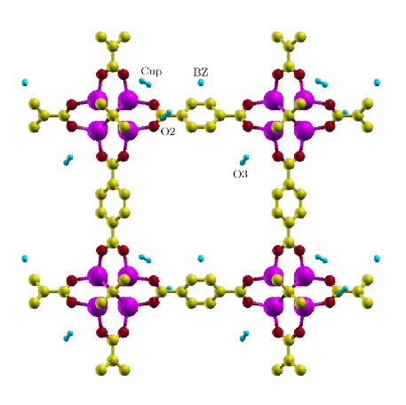
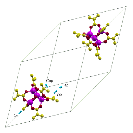
Figure S1: Illustration of H₂ adsorption sites in MOF-5 unit cell (top) and primitive cell (bottom). MOF-5 has FCC structure with lattice constant of 25.89Å Rowselljacs2005 . The primitive cell has 106 atoms. The H atoms on benzene rings are omitted for clarity.

The four type of adsorption sites are shown in Fig. S1. To calculate the stretch frequency for H₂ at each of these four sites, we performed a series of calculations varying the bond length of H₂, with the center of H₂ and the host atoms fixed at their equilibrium positions. The resulting potential-energy curve was used in the Schrödinger equation to obtain the eigenvalues and excitation frequencies. A similar calculation was also carried out for isolated H₂ to obtain the frequency shift due to MOF-H₂ interaction. The ab initio total energies vs H₂ internuclear distance were tabulated in Tables S3$-$S6 for H₂ at the four type of adsorption sites.

Rotational frequency

In order to calculate the rotational states, we first sample the solid angle to get the total energies. The spherical surface was sampled as follows: the polar angle were evenly divided into seven layers; and the azimuthal angle were then sampled by {1,8,16,24,16,8,1} number of points corresponding to each layer from pole to pole of the sphere. We next fit these potential energies with spherical harmonics

$$V(\theta,\phi)=\sum_{lm}c_{lm}Y_{lm}$$ (S1)

which was then substituted into the rigid rotor equation and diagonalized for rotational energies. We found that fitting with $s$ and $d$ states gave results converged within 1 cm^-1. The fitted coefficients are shown in Table S7. The calculated rotational energy states are shown in Tables S8$-$S11.

Wannier function approach for dipole moment and IR intensity

The Wannier functions were calculated with the Wannier90 code Wannier90 embedded in ABINIT and the Brillouin zone was sampled by a 2x2x2 Monkhorst-Pack grid. The Wannier centers for the bare MOF were first calculated and used as initial guess for the H₂ loaded system. The change of MOF Wannier centers upon H₂ adsorption was obtained from

$$\delta\mathbf{r}_{n}=\mathbf{r}^{MOF+H_{2}}_{n}-\mathbf{r}^{MOF}_{n}$$ (S2)

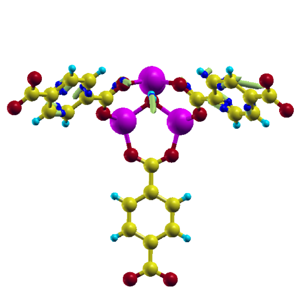
Figure S3: Illustration of the O2 adsorption site and the change of Wannier centers due to H₂ adsorption compared to bare MOF and free H₂. The vector lengths are enlarged by 1200.

where $\mathbf{r}_{n}$ is the center of the $n$-th Wannier function. Fig. S3$-$S5 show these changes for the O2, O3 and benzene sites while the cup site is given in the main text.

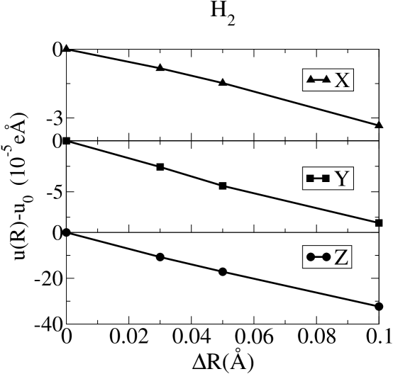
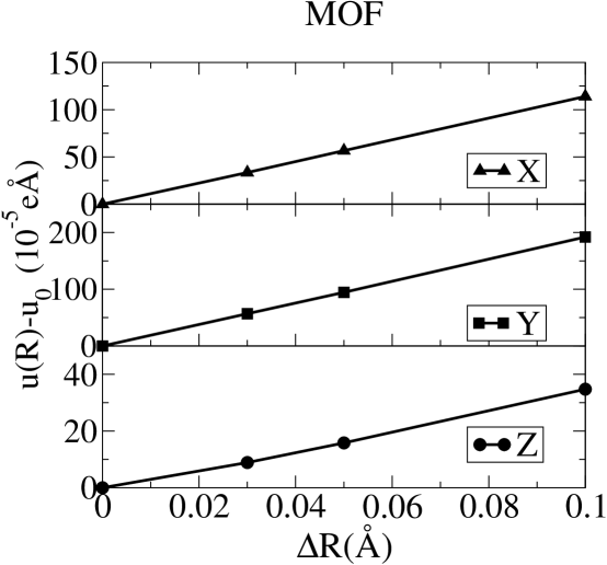
Figure S6: $\delta{\mathbf{u}}$ as a function of H₂ internuclear distance. u₀ is the dipole at equilibrium distance.

To calculate the IR intensity, one first needs to get the derivative of the dipole with respect to the normal coordinates corresponding to H₂ stretch vibration. We used the H₂ internuclear distance as an approximation for the stretching normal coordinates and the derivative was approximate by the finite difference. To reduce the numerical errors, the bond stretching should be sufficiently large, but still in the linear regime. We found that a stretch of 0.05A from equilibrium bond length was appropriate, as shown in Fig. S6.

Model for induced dipole

The total induced dipole of the system can be approximated by a sum of four terms.

$$\mathbf{u}=\mathbf{u}^{H_{2}}_{0}+\mathbf{u}^{MOF}_{0}+\mathbf{u}^{MOF}_{1}+\mathbf{u}^{H_{2}}_{1}$$ (S3)

The first term on the right-hand side is the induced dipole on H₂ due to interactions with MOF atoms. The second term is the induced dipole on MOF atoms due to H₂ quadrupole. The third term is the induced dipole on MOF due to $\mathbf{u}^{H_{2}}_{0}$ and the fourth term is the induced dipole on H₂ due to $\mathbf{u}^{MOF}_{0}$. These last two terms are second order corrections. We now derive the expressions for the four terms for cup site adsorption.

.1 $\mathbf{u}^{H_{2}}_{0}$

Due to the 3-fold symmetry, the electric field ($\vec{E}$) at cup site due to MOF atoms is along the rotation axis, i.e. Z. For H₂ with its bond oriented along ($\theta,\phi$), the projected fields along and perpendicular to the bond are

$$E_{\|} =E\cos\theta$$ (S4a)

$$E_{\bot} =E\sin\theta$$ (S4b)

and the corresponding induced dipole is

$$u_{\|} =E\alpha_{\|}\cos\theta$$ (S5a)

$$u_{\bot} =E\alpha_{\bot}\sin\theta$$ (S5b)

where $\alpha_{\|}$ and $\alpha_{\bot}$ are the H₂ polarizability along and perpendicular to the bond. In Cartesian coordinates, this gives

$$u_{0X}^{H_{2}} =E(\alpha_{\|}-\alpha_{\bot})\sin\theta\cos\theta\cos\phi$$ (S6a)

$$u_{0Y}^{H_{2}} =E(\alpha_{\|}-\alpha_{\bot})\sin\theta\cos\theta\sin\phi$$ (S6b)

$$u_{0Z}^{H_{2}} =E(\alpha_{\|}\cos^{2}\theta+\alpha_{\bot}\sin^{2}\theta)$$ (S6c)

.2 $\mathbf{u}^{MOF}_{0}$

Hydrogen molecule has permanent quadrupole. The tensor is $Q_{zz}=-2Q_{xx}=-2Q_{yy}=Q$. For H₂ at origin with orientation of ($\theta,\phi$), the quadrupole potential at position P₁(X,Y,Z) is

$$V(\mathbf{r})=\frac{3Q}{2r^{5}}\tilde{Z}^{2}-\frac{Q}{2r^{2}}$$ (S7)

where $r=(X^{2}+Y^{2}+Z^{2})^{1/2}$ and $\tilde{Z}=X\sin\theta\cos\phi+Y\sin\theta\sin\phi+Z\cos\theta$. The electric field of this potential is

$$E_{0X}(\mathbf{r}) =\frac{3Q}{2r^{7}}\left\{-2r^{2}\sin\theta\cos\phi\tilde{Z}+5X\tilde{Z}^{2}\right\}-\frac{3Q}{2r^{5}}X$$ (S8a)

$$E_{0Y}(\mathbf{r}) =\frac{3Q}{2r^{7}}\left\{-2r^{2}\sin\theta\sin\phi\tilde{Z}+5Y\tilde{Z}^{2}\right\}-\frac{3Q}{2r^{5}}Y$$ (S8b)

$$E_{0X}(\mathbf{r}) =\frac{3Q}{2r^{7}}\left\{-2r^{2}\sin\theta\cos\phi\tilde{Z}+5Z\tilde{Z}^{2}\right\}-\frac{3Q}{2r^{5}}Z$$ (S8c)

The MOF charge density will be shifted by this field and thus leads to induced dipole. To calculate this induced dipole on MOF, one may view that there is an electron at position P₁ with partial charge which is equal to the charge density at P₁. This charge has a certain polarizability. The total induced dipole can then be formally calculated by multiplying the electric field by the corresponding polarizability and then integrating over the whole MOF space. This procedure is somewhat an extension of the classical point charge into the continuous charge density regime. Assuming the polarizability is isotropic, the final result will have the same dependence on ($\theta,\phi$) as electric field since the integration runs over (X,Y,Z) while ($\theta,\phi$) will be left unchanged. In other words, we will have an equation of the form in Eq. (5) in the main text. Note that the isotropic assumption is not critical here except in making the final equations simpler. If one had used the whole polarizability tensor, the final result can still be cast into the form in Eq. (5) in the main text. We found that the isotropic assumption gave consistent results for our system.

Due to the 3-fold rotation symmetry, there are three equivalent points with equal polarizability in MOF. Taking advantage of this symmetry, the sum of the electric fields at the three positions is

$$\tilde{E}_{0X} =\frac{9Q}{4r^{7}}\left\{\left(3r^{2}-5Z^{2}\right)Z\sin 2\theta\cos\phi-\frac{5}{2}\left(3XY^{2}-X^{3}\right)\sin^{2}\theta\cos 2\phi+\frac{5}{2}\left(3X^{2}Y-Y^{3}\right)\sin^{2}\theta\sin 2\phi\right\}$$ (S9a)

$$\tilde{E}_{0Y} =\frac{9Q}{4r^{7}}\left\{\left(3r^{2}-5Z^{2}\right)Z\sin 2\theta\sin\phi+\frac{5}{2}\left(3X^{2}Y-Y^{3}\right)\sin^{2}\theta\cos 2\phi+\frac{5}{2}\left(3XY^{2}-X^{3}\right)\sin^{2}\theta\sin 2\phi\right\}$$ (S9b)

$$\tilde{E}_{0Z} =\frac{9Q}{4}\frac{(5Z^{2}-3r^{2})Z}{r^{7}}(3\cos^{2}\theta-1)$$ (S9c)

The induced dipole on MOF is therefore given by

$$u_{0X}^{MOF} =C_{01}^{MOF}\sin 2\theta\cos\phi-C_{02}^{MOF}\sin^{2}\theta\cos 2\phi+C_{03}^{MOF}\sin^{2}\theta\sin 2\phi$$ (S10a)

$$u_{0Y}^{MOF} =C_{01}^{MOF}\sin 2\theta\sin\phi+C_{03}^{MOF}\sin^{2}\theta\cos 2\phi+C_{02}^{MOF}\sin^{2}\theta\sin 2\phi$$ (S10b)

$$u_{0Z}^{MOF} =C_{04}^{MOF}(3\cos^{2}\theta-1)$$ (S10c)

where

$$C_{01}^{MOF} =\int\frac{9Q}{4r^{7}}\left(3r^{2}-5Z^{2}\right)Z\alpha^{MOF}(\mathbf{r})\,d\mathbf{r}$$ (S11a)

$$C_{02}^{MOF} =\int\frac{9Q}{4r^{7}}\frac{5}{2}\left(3XY^{2}-X^{3}\right)\alpha^{MOF}(\mathbf{r})\,d\mathbf{r}$$ (S11b)

$$C_{03}^{MOF} =\int\frac{9Q}{4r^{7}}\frac{5}{2}\left(3X^{2}Y-Y^{3}\right)\alpha^{MOF}(\mathbf{r})\,d\mathbf{r}$$ (S11c)

$$C_{04}^{MOF} =\int\frac{9Q}{4r^{7}}(5Z^{2}-3r^{2})Z\alpha^{MOF}(\mathbf{r})\,d\mathbf{r}$$ (S11d)

and the integration runs over the 1/3 irreducible region of MOF, as a result of the 3-fold rotation symmetry.

.3 2^nd-order corrections: $\mathbf{u}^{MOF}_{1}$ and $\mathbf{u}^{H_{2}}_{1}$

The induced dipole on H₂ and MOF, $\mathbf{u}^{H_{2}}_{0}$ and $\mathbf{u}^{MOF}_{0}$, further induces dipole on each other and produces second order corrections. For $\mathbf{u}^{H_{2}}_{0}$, it gives electric field at P₁(X,Y,Z)

$$E_{1X}(\mathbf{r}) =\frac{1}{r^{5}}\left(-u^{H_{2}}_{0X}r^{2}+3\mathbf{u}^{H_{2}}_{0}\cdot\mathbf{r}X\right)$$ (S12a)

$$E_{1Y}(\mathbf{r}) =\frac{1}{r^{5}}\left(-u^{H_{2}}_{0Y}r^{2}+3\mathbf{u}^{H_{2}}_{0}\cdot\mathbf{r}Y\right)$$ (S12b)

$$E_{1Z}(\mathbf{r}) =\frac{1}{r^{5}}\left(-u^{H_{2}}_{0Z}r^{2}+3\mathbf{u}^{H_{2}}_{0}\cdot\mathbf{r}Z\right)$$ (S12c)

Similar to the derivation of $\mathbf{u}^{MOF}_{0}$, one obtains

$$u^{MOF}_{1X} =C_{11}^{MOF}\sin 2\theta\cos\phi-C_{12}^{MOF}\sin^{2}\theta\cos 2\phi+C_{13}^{MOF}\sin^{2}\theta\sin 2\phi$$ (S13a)

$$u^{MOF}_{1Y} =C_{11}^{MOF}\sin 2\theta\sin\phi+C_{12}^{MOF}\sin^{2}\theta\sin 2\phi+C_{13}^{MOF}\sin^{2}\theta\cos 2\phi$$ (S13b)

$$u^{MOF}_{1Z} =C_{14}^{MOF}\cos^{2}\theta+C_{15}^{MOF}$$ (S13c)

where

$$C_{11}^{MOF} =\int\left\{\frac{9Q}{4}\left(\frac{3Z}{r^{5}}-\frac{5Z^{3}}{r^{7}}\right)+\frac{3E}{4}\left(\frac{1}{r^{3}}-\frac{3Z^{2}}{r^{5}}\right)\left(\alpha_{\|}-\alpha_{\perp}\right)\right\}\alpha^{MOF}(\mathbf{r})\,d\mathbf{r}$$ (S14a)

$$C_{12}^{MOF} =\int\left\{\frac{45Q}{8r^{7}}\left(3XY^{2}-X^{3}\right)\right\}\alpha^{MOF}(\mathbf{r})\,d\mathbf{r}$$ (S14b)

$$C_{13}^{MOF} =\int\left\{\frac{45Q}{8r^{7}}\left(3X^{2}Y-Y^{3}\right)\right\}\alpha^{MOF}(\mathbf{r})\,d\mathbf{r}$$ (S14c)

$$C_{14}^{MOF} =\int\left\{\frac{27Q}{4}\left(-\frac{3Z}{r^{5}}+\frac{5Z^{3}}{r^{7}}\right)-3E\left(\frac{1}{r^{3}}-\frac{3Z^{2}}{r^{5}}\right)(\alpha_{\|}-\alpha_{\perp})\right\}\alpha^{MOF}(\mathbf{r})\,d\mathbf{r}$$ (S14d)

$$C_{15}^{MOF} =\int\left\{\frac{9Q}{4}\left(\frac{3Z}{r^{5}}-\frac{5Z^{3}}{r^{7}}\right)-3E\left(\frac{1}{r^{3}}-\frac{3Z^{2}}{r^{5}}\right)\alpha_{\perp}\right\}\alpha^{MOF}(\mathbf{r})\,d\mathbf{r}$$ (S14e)

and the integration again runs over 1/3 of the MOF region.

Now let us look at the second-order correction on H₂, $\mathbf{u}^{H_{2}}_{1}$. The hydrogen quadrupole generates electric field at P₁ as given by Eq. (S9). With the help of the partial charge and local polarizability concept, this field produces a local dipole $\mathbf{u}^{MOF}_{0}(\mathbf{r})=\alpha^{MOF}(\mathbf{r})\mathbf{E}_{0}(\mathbf{r})$ where $\mathbf{E}_{0}$($\mathbf{r}$) is given in Eq. (S8) and $\alpha^{MOF}(\mathbf{r})$ is assumed to be isotropic. The electric field back at H₂ due to this local dipole is

$$E^{H_{2}}_{1X} =-\frac{\alpha}{r^{5}}\left\{E^{MOF}_{0X}(r^{2}-3X^{2})-3E^{MOF}_{0Y}XY-3E^{MOF}_{0Z}XZ\right\}$$ (S15a)

$$E^{H_{2}}_{1Y} =-\frac{\alpha}{r^{5}}\left\{E^{MOF}_{0Y}(r^{2}-3Y^{2})-3E^{MOF}_{0X}XY-3E^{MOF}_{0Z}YZ\right\}$$ (S15b)

$$E^{H_{2}}_{1Z} =-\frac{\alpha}{r^{5}}\left\{E^{MOF}_{0Z}(r^{2}-3Z^{2})-3E^{MOF}_{0X}XZ-3E^{MOF}_{0Y}YZ\right\}$$ (S15c)

Inserting Eq. (S9) into Eq. (S15), adding together the three rotationally equivalent points and integrating over the 1/3 MOF region, one finally obtains

$$\tilde{E}^{H_{2}}_{1X} =C^{H_{2}}_{11}\sin 2\theta\cos\phi-C^{H_{2}}_{12}\sin^{2}\theta\cos 2\phi+C^{H_{2}}_{13}\sin^{2}\theta\sin 2\phi$$ (S16a)

$$\tilde{E}^{H_{2}}_{1Y} =C^{H_{2}}_{11}\sin 2\theta\cos\phi+C^{H_{2}}_{12}\sin^{2}\theta\sin 2\phi+C^{H_{2}}_{13}\sin^{2}\theta\cos 2\phi$$ (S16b)

$$\tilde{E}^{H_{2}}_{1Z} =C^{H_{2}}_{14}\cos^{2}\theta+C^{H_{2}}_{15}$$ (S16c)

where

$$C^{H_{2}}_{11} =\int\frac{9\alpha^{MOF}(\mathbf{r})QZ}{2r^{8}}\left(\frac{33}{16}-\frac{Z^{2}}{8r^{2}}-\frac{15Z^{4}}{16r^{4}}-\frac{5X^{2}Y^{2}}{4r^{4}}\right)\,d\mathbf{r}$$ (S17a)

$$C^{H_{2}}_{12} =\int\frac{9\alpha^{MOF}(\mathbf{r})Q}{2r^{10}}(3Y^{2}-X^{2})X\,d\mathbf{r}$$ (S17b)

$$C^{H_{2}}_{13} =\int\frac{9\alpha^{MOF}(\mathbf{r})Q}{2r^{10}}(3X^{2}-Y^{2})Y\,d\mathbf{r}$$ (S17c)

$$C^{H_{2}}_{14} =\int\frac{9\alpha^{MOF}(\mathbf{r})QZ}{2r^{8}}\left(-\frac{9}{16}+\frac{45}{8}\frac{Z^{2}}{r^{2}}+\frac{15}{16}\frac{Z^{4}}{r^{4}}+\frac{5X^{2}Y^{2}}{4r^{4}}\right)\,d\mathbf{r}$$ (S17d)

$$C^{H_{2}}_{15} =\int\frac{9\alpha^{MOF}(\mathbf{r})QZ}{2r^{8}}\left(\frac{57}{16}-\frac{37}{8}\frac{Z^{2}}{r^{2}}-\frac{15}{16}\frac{Z^{4}}{r^{4}}-\frac{5X^{2}Y^{2}}{4r^{4}}\right)\,d\mathbf{r}$$ (S17e)

and the integral is over the 1/3 of the MOF space. Considering the anisotropy of the polarizability of H₂, we have

$$\mathbf{u}^{H_{2}}_{1}\\ =\left[\alpha_{\perp}+(\alpha_{\|}-\alpha_{\perp})\left(\begin{array}[]{lll}\sin^{2}\theta\cos^{2}\phi&\sin^{2}\theta\sin\phi\cos\phi&\sin\theta\cos\theta\cos\phi\\ \sin^{2}\theta\sin\phi\cos\phi&\sin^{2}\theta\sin^{2}\phi&\sin\theta\cos\theta\sin\phi\\ \sin\theta\cos\theta\cos\phi&\sin\theta\cos\theta\sin\phi&\cos^{2}\theta\end{array}\right)\right]\tilde{\mathbf{E}}^{H_{2}}_{1}$$ (S18)

The anisotropic term impose a small correction to the first term inside the bracket. For simplicity, we neglect the second term so that $\mathbf{u}^{H_{2}}_{1}$ and $\tilde{\mathbf{E}}^{H_{2}}_{1}$ have a simple linear relationship. In particular, they have the same form of dependence on ($\theta,\phi$) as given in Eq. (S16).

.4 Coefficients

From Eq. (S6), (S10), (S13) and (S16), we conclude that the following equations hold

$$u^{s}_{X} =C_{1}^{s}\sin 2\theta\cos\phi-(C_{2}^{s}\cos 2\phi-C_{3}^{s}\sin 2\phi)\sin^{2}\theta$$ (S19a)

$$u^{s}_{Y} =C_{1}^{s}\sin 2\theta\sin\phi+(C_{2}^{s}\sin 2\phi+C_{3}^{s}\cos 2\phi)\sin^{2}\theta$$ (S19b)

$$u^{s}_{Z} =C_{4}^{s}\cos^{2}\theta+C_{5}^{s}$$ (S19c)

where $s$ denotes the system and could be H₂, MOF or the total. To determine the coefficients C’s, we calculated the dipole and the derivative of the dipole with respect to H₂ internuclear distance with Wannier function approach for five hydrogen orientations. The Z components of the obtained values were used to fit C₄ and C₅ in Eq. (S19c). As shown in Fig. S7, good linearity is obtained in agreement with our model.

To compute C₁, C₂ and C₃, we pick three ab initio calculated value, u${}^{\prime}_{x}$/u${}^{\prime}_{y}$ of orientation 4 and u${}^{\prime}_{x}$ of orientation 5, to solve a 3$\times$3 linear equation for the coefficients. To check the values obtained, we substitute them back into Eq. (S19a) and (S19b) for other orientations and compare with the ab initio results. The comparison are shown in Table S12 and S13. Consistent results are obtained generally while we do see some deviations on the induced dipole on H₂, which may be due to the neglect of the anisotropy in Eq. (S18). However, the absolute magnitude of these deviations are quite small ($<$ 10%) compared to the total value which is the sum of the induced dipole on MOF and on H₂.

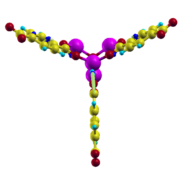
Figure S4: Illustration of the O3 adsorption site and the change of Wannier centers due to H₂ adsorption compared to bare MOF and free H₂. The vector lengths are enlarged by 1200.

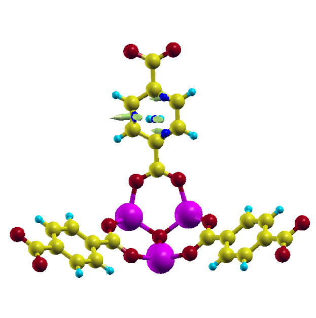
Figure S5: Illustration of the benzene adsorption site and the change of Wannier centers due to H₂ adsorption compared to bare MOF and free H₂. The vector lengths are enlarged by 1200.

Table S3: Calculated total energy vs H₂ internuclear distance at cup site

R(a.u.)	E(a.u.)
0.63258	-1147.23459646
0.70817	-1147.34182739
0.78376	-1147.41767267
0.85935	-1147.47155388
0.93494	-1147.50972612
1.01052	-1147.53646724
1.08611	-1147.55478553
1.16170	-1147.56683964
1.23729	-1147.57419775
1.31288	-1147.57801104
1.38847	-1147.57913028
1.48297	-1147.57768502
1.57745	-1147.57390705
1.67194	-1147.56843515
1.76642	-1147.56176098
1.86091	-1147.55423624
1.95540	-1147.54614531
2.04988	-1147.53771266
2.14437	-1147.52910151
2.23886	-1147.52044322
2.33334	-1147.51183591

Table S4: Calculated total energy vs H₂ internuclear distance at O2 site

R(a.u.)	E(a.u.)
0.63142	-1147.23167787
0.70701	-1147.33946050
0.78259	-1147.41567703
0.85818	-1147.46981324
0.93377	-1147.50816182
1.00936	-1147.53502878
1.08495	-1147.55343531
1.16054	-1147.56555111
1.23613	-1147.57295236
1.31172	-1147.57679567
1.38731	-1147.57793396
1.48182	-1147.57650225
1.57630	-1147.57273083
1.67079	-1147.56726718
1.76528	-1147.56059280
1.85976	-1147.55307608
1.95425	-1147.54499838
2.04873	-1147.53657940
2.14322	-1147.52798691
2.23771	-1147.51934958
2.33219	-1147.51076491

Table S5: Calculated total energy vs H₂ internuclear distance at O3 site

R(a.u.)	E(a.u.)
0.63117	-1147.23131641
0.70676	-1147.33921650
0.78235	-1147.41551509
0.85794	-1147.46970566
0.93353	-1147.50809162
1.00912	-1147.53498512
1.08471	-1147.55340776
1.16030	-1147.56553250
1.23589	-1147.57293612
1.31147	-1147.57677507
1.38705	-1147.57790325
1.48153	-1147.57645368
1.57601	-1147.57265607
1.67050	-1147.56716130
1.76499	-1147.56045531
1.85947	-1147.55290340
1.95396	-1147.54478993
2.04845	-1147.53633172
2.14293	-1147.52769561
2.23742	-1147.51900844
2.33191	-1147.51036692

Table S6: Calculated total energy vs H₂ internuclear distance at benzene site

R(a.u.)	E(a.u.)
0.63097	-1147.23028851
0.70656	-1147.33826702
0.78215	-1147.41460791
0.85774	-1147.46882070
0.93333	-1147.50721490
1.00891	-1147.53410287
1.08450	-1147.55251525
1.16009	-1147.56462548
1.23568	-1147.57201447
1.31127	-1147.57584010
1.38686	-1147.57695620
1.48135	-1147.57549948
1.57583	-1147.57170006
1.67032	-1147.56620858
1.76480	-1147.55950504
1.85929	-1147.55195560
1.95378	-1147.54384388
2.04826	-1147.53538984
2.14275	-1147.52676285
2.23724	-1147.51809406

Table S7: Expansion coefficients (meV) of orientational potential energy surface in the basis of spherical harmonics. The equilibrium energy is set to be zero.

site	s	$d_{z^{2}}$	$d_{xz}$	$d_{yz}$	$d_{xy}$	$d_{x^{2}-y^{2}}$
cup	17.0	0.06	8.45	8.41	8.55	-0.006
O2	25.0	-3.74	-6.36	-6.90	-5.76	-4.88
O3	7.73	0.27	-2.43	-2.39	-2.38	0
benzene	1.46	-0.52	0	0.27	0	0.80

Table S8: Rotational eigen energies (meV) at cup site

State #	Energy	Ei-E1	j	m
1	4.428	–	0	0
2	17.498	13.070	1	$-$1
3	17.555	13.127		1
4	23.014	18.586		0
5	46.197	41.769	2	$-$2
6	46.197	41.769		2
7	50.094	45.666		$-$1
8	50.135	45.707		1
9	51.781	47.353		0
10	89.88	85.452	3	$-$3
11	89.88	85.452		3
12	92.934	88.506		$-$2
13	92.934	88.506		2
14	94.856	90.428		$-$1
15	94.894	90.466		1
16	95.552	91.124		0

Table S9: Rotational eigen energies (meV) at O2 site

State #	Energy	Ei-E1
1	6.76	–
2	18.614	11.854
3	22.306	15.546
4	24.03	17.270
5	49.036	42.276
6	49.39	42.630
7	50.619	43.859
8	53.265	46.505
9	53.439	46.679
10	93.026	86.266
11	93.146	86.386
12	94.315	87.555
13	95.211	88.451
14	95.488	88.728
15	97.788	91.028
16	97.801	91.041

Table S10: Rotational eigen energies (meV) at O3 site

State #	Energy	Ei-E1	j	m
1	2.148	–	0	0
2	15.815	13.667	1	0
3	17.356	15.208		$-$1
4	17.434	15.286		1
5	45.551	43.403	2	0
6	45.869	43.721		$-$1
7	45.924	43.776		1
8	47.026	44.878		$-$2
9	47.027	44.879		2
10	89.685	87.537	3	0
11	89.831	87.683		$-$1
12	89.884	87.736		1
13	90.375	88.227		$-$2
14	90.377	88.229		2
15	91.253	89.105		$-$3
16	91.253	89.105		3

Table S11: Rotational eigen energies (meV) at benzene site

State #	Energy	Ei-E1
1	0.409	–
2	14.929	14.520
3	15.051	14.642
4	15.35	14.941
5	44.332	43.923
6	44.339	43.930
7	44.553	44.144
8	44.64	44.231
9	44.691	44.282
10	88.408	87.999
11	88.409	88.000
12	88.595	88.186
13	88.611	88.202
14	88.693	88.284
15	88.773	88.364
16	88.787	88.378

Table S12: Comparison of ($\delta u_{X},\delta u_{Y}$) on MOF due to H₂ bond stretching of 0.05Å between the ab initio and the fitted values

orientation	$\theta$(degree)	$\phi$(degree)	ab initio		fitted
			$\delta u_{x}$	$\delta u_{y}$	$\delta u_{x}$	$\delta u_{y}$
1	99.650	-95.723	5.690E-04	9.440E-04	5.690E-04	9.634E-04
2	87.054	-6.190	-4.864E-04	-8.400E-04	-5.178E-04	-8.720E-04
3	10.097	-112.811	-5.760E-05	-1.008E-04	-5.172E-05	-9.052E-05
4	54.741	-98.278	2.774E-04	2.464E-04	–	–
5	42.937	-16.295	2.640E-04	-6.126E-04	–	-5.754E-04

Table S13: comparison of ($\delta u_{X},\delta u_{Y}$) on H₂ due to bond stretching of 0.05Å between the ab initio and the fitted values

orientation	$\theta$(degree)	$\phi$(degree)	ab initio		fitted
			$\delta u_{x}$	$\delta u_{y}$	$\delta u_{x}$	$\delta u_{y}$
1	99.650	-95.723	-1.631E-05	-4.322E-05	-2.286E-05	-6.552E-05
2	87.054	-6.190	1.562E-05	2.220E-05	1.340E-05	4.522E-05
3	10.097	-112.811	1.338E-05	3.052E-05	9.392E-06	2.030E-05
4	54.741	-98.278	-2.190E-06	3.340E-05	–	–
5	42.937	-16.295	-6.386E-05	3.326E-05	–	4.184E-05

Table S14: Theory vs experiment (Ref. FitzGerald2008, ) for RV frequency shifts (cm^-1) of adsorbed H₂ relative to free H₂. The vibrational transition is from the ground state to the 1st excited state ($v$=0 $\rightarrow$ $v$=1).

site		S(0) (para)	S(1) (ortho)
		($j$=0$\rightarrow j$=2)	($j$=1$\rightarrow j$=3)
O2	Th.	$-37$, $-34$, $-24$, $-3$, $-1$	$-15$, $-14$, $-4,3$, $5$, $24$, $24$
	Ex.	$-36.7$, $-27.3$, $-24.3$, $-7.4$	$-12.9$
O3	Th.	$-19$, $-16$, $-7$	$-10$, $-9$, $-4$, $3$

Table S15: Angular integral $\langle jm|\mathbf{u^{\prime}}|jm\rangle$ for H₂ at cup site. The energy of the $|00\rangle$ is set as reference. The units for $\mathbf{u^{\prime}}$ is 10^-3e.

jm	u${}^{\prime}_{X}$	u${}^{\prime}_{Y}$	u${}^{\prime}_{Z}$	u${}^{\prime 2}(\times 10^{-6}e^{2})$	E(meV)
00	-0.009	0.02	-2.23	5.0	0
1$\bar{1}$	-2.38	7.69	-1.41	66.7	13.1
11	2.36	-7.67	-1.40	66.4	13.2
10	0.003	0.01	-4.67	21.8	18.6

Table S16: Theoretical predictions and experimental data FitzGerald2008 for $v=0\rightarrow v=1$ transitions of H₂ at the cup site. The frequency shift $\Delta$v (cm^-1) is relative to the corresponding free H₂ value and the angular integral given by $I_{A}^{2}=|\langle j_{f}m_{f}|\mathbf{u^{\prime}}|j_{i}m_{i}\rangle|^{2}$ (10^-6e²). The rotational energy (meV) $E^{rot}_{i}$ of the $|00\rangle$ state is set as a reference. The theoretical intensity is calculated from $I_{A}^{2}$ weighted by the 30K Boltzmann factor and the spin ratio of 1:3 between para and ortho H₂. The strongest line is normalized to 100.

	mi	mf	Theory				Experiment
			E${}_{i}^{rot}$	$\Delta$v	$I^{2}_{A}$	Intensity	$\Delta$v	Intensity
Q(0)($j_{i}$=0$\rightarrow j_{f}$=0)	0	0	0	-23	5	2		absent
Q(1)($j_{i}$=1$\rightarrow j_{f}$=1)	$\pm 1$	$\pm 1$	13.1	-23	66	97	$-$27.5	strong
	0	0	18.6		22
Q*(1)($j_{i}$=1$\rightarrow j_{f}$=1)	$\pm 1$	0	13.1	22	6	9	39	weak
S(0) ($j_{i}$=0$\rightarrow j_{f}$=2)	0	$\pm$2	13.1	$-$44	115	58	$-$49.3	strong
		$\pm$1		$-12$	10	5	$-$6.8	weak
		0		$-$1	5	2		absent
S(1)($j_{i}$=1$\rightarrow j_{f}$=3)	$\pm 1$	$\pm$3	13.1	$-$34	69	100	$-$36.8	strong
		$\pm$2		$-$9	4	6	$-$0.8	weak
		$\pm$1		6	6	9	21.6	weak
		0		11	2	3		absent
	0	$\pm$3	18.6	$-$78	0	0		absent
		$\pm$2		$-$53	49	3	$-$61	weak
		$\pm$1		$-$50	8	$\sim$0		absent
		0		$-$33	6	$\sim$0		absent

References

- (1) Y. J. Chabal and C. K. N. Patel, Phys. Rev. Lett. 53, 210 (1984).
- (2) M. Dion et al., Phys. Rev. Lett. 92, 246401 (2005); T. Thonhauser et al., Phys. Rev. B 76, 125112 (2007); G. Román-Pérez and J. Soler, Phys. Rev. Lett. 103, 096102 (2009).
- (3) R. D. King-Smith and D. Vanderbilt, Phys. Rev. B, 47, 1651 (1993).
- (4) N. Marzari and D. Vanderbilt, Phys. Rev. B, 56, 12847 (1997); I. Souza et al., Phys. Rev. B, 62, 15505 (2000).
- (5) N. L. Rosi et al., Science 300, 1127 (2003).
- (6) L. J. Murray, M. Dincǎ, and J. R. Long, Chem. Soc. Rev. 38, 1294 (2009).
- (7) A. U. Czaja, N. Trukhan, and U. Müller, Chem. Soc. Rev. 38, 1284 (2009).
- (8) S. A. FitzGerald et al., Phys. Rev. B 77, 224301 (2008).
- (9) J. L. C. Rowsell et al., Science 309, 1350 (2005).
- (10) L. Kong et al., Phys. Rev. B 79, 081407 (2009).
- (11) L. Kong, G. Román-Pérez, J. M. Soler, and D. C. Langreth, Phys. Rev. Lett. 103, 096103 (2009).
- (12) T. Yildirim and M. R. Hartman, Phys. Rev. Lett. 95, 215504 (2005).
- (13) K. Sillar, A. Hofmann, and J. Sauer, J. Am. Chem. Soc. 131, 4143 (2009).
- (14) D. C. Langreth et al., J. Phys.: Cond. Mat. 21, 084203 (2009).
- (15) K. Lee et al., Phys. Rev. B 82, 081101 (2010).
- (16) J. L. C. Rowsell, J. Eckert, and O. M. Yaghi, J. Am. Chem. Soc. 127, 14904 (2005).
- (17) S. A. FitzGerald, S. Forth, and M. Rinkoski, Phys. Rev. B 65, 140302 (2002).
- (18) J. L. C. Rowsell and O. M. Yaghi, J. Am. Chem. Soc. 128, 1304 (2006).
- (19) S. S. Kaye and J. R. Long, J. Am. Chem. Soc. 127, 6506 (2005).
- (20) S. A. FitzGerald et al., Phys. Rev. B 81, 104305 (2010).

References

- (1) X. Gonze et al., Comp. Mat. Sci. 25, 478 (2002). X. Gonze, et al. Z. Kristallogr. 220, 558 (2005).
- (2) P. Ordejón, E. Artacho and J. M. Soler, Phys. Rev. 53, 10441(R) (1996); J. M. Soler, E. Artacho, J. D. Gale, A. García, J. Junquera, P. Ordejón, and D. Sánchez-Portal, J. Phys.: Condens. Matt. 14, 2745 (2002).
- (3) N. Troullier; J. L. Martins, Phys. Rev. B 43, 1991 (1993).
- (4) A. A. Mostofi, J. R. Yates, Y.-S Lee, I. Souza, D. Vanderbilt, N. Marzari, Comput. Phys. Commun. 178, 685 (2008).
- (5) S. FitzGerald, K. Allen, P. Landerman, J. Hopkins, J. Matters, R. Myers, and J. L. C. Rowsell, Phys. Rev. B, 77, 224301 (2008).
- (6) J. L. C. Rowsell, J. Eckert, and O. M. Yaghi, J. Am. Chem. Soc. 127, 14904 (2005).