Probabilistic cellular automata, invariant measures,
and perfect sampling

Abstract

A probabilistic cellular automaton (PCA) can be viewed as a Markov chain. The cells are updated synchronously and independently, according to a distribution depending on a finite neighborhood. We investigate the ergodicity of this Markov chain. A classical cellular automaton is a particular case of PCA. For a 1-dimensional cellular automaton, we prove that ergodicity is equivalent to nilpotency, and is therefore undecidable. We then propose an efficient perfect sampling algorithm for the invariant measure of an ergodic PCA. Our algorithm does not assume any monotonicity property of the local rule. It is based on a bounding process which is shown to be also a PCA. Last, we focus on the PCA Majority, whose asymptotic behavior is unknown, and perform numerical experiments using the perfect sampling procedure.

Keywords: probabilistic cellular automata, perfect sampling, invariant measures, ergodicity.

AMS classification (2010): Primary: 37B15, 60J05, 60J22. Secondary: 37A25, 60K35, 68Q80.

1 Introduction

A deterministic cellular automaton (DCA) consists of a lattice (e.g. $\mathbb{Z}$ or $\mathbb{Z}^{2}$ or $\mathbb{Z}/n\mathbb{Z}$) divided in regular cells, each cell containing a letter of a finite alphabet. The cells evolve synchronously, each one evolving in function of a finite number of cells in its neighborhood, according to a local rule.

DCA form a natural mathematical object: by Hedlund’s theorem [18], the mappings realized by DCA are precisely the continuous functions (for the product topology) commuting with the shift. They also constitute a powerful model of computation, in particular they can “simulate” any Turing machine. Last, due to the amazing gap between the simplicity of the definition and the intricacy of the generated behaviors, DCA are good candidates for modelling “complex systems” appearing in physical and biological processes.

Probabilistic cellular automata. To take into account random events, one is led to consider probabilistic versions of DCA. In one of them, at most one cell is updated at each time, this cell being randomly chosen according to a given distribution. For an infinite set of cells, one is led to consider continuous time models, obtaining what is known in probability theory as an interacting particle system [23]. Another model is that of probabilistic cellular automata (PCA) [31]. For PCA, time is discrete, and all the cells evolve synchronously as for DCA, but the difference is that for each cell, the new content is randomly chosen, independently of the others, according to a distribution depending only on a finite neighborhood of the cell.

Let us mention a couple of motivations. First, the investigation of fault-tolerant computational models was the motivation for the Russian school to study PCA [31, 12]. Second, PCA appear in combinatorial problems related to the enumeration of directed animals [9, 2, 22]. Third, in the context of the classification of DCA (Wolfram’s program), robustness to random errors can be used as a discriminating criterion [11, 26]. Recently, PCA also proved to be pertinent for the density classification problem [10], that is, testing efficiently if some sequence contains more occurrences of $0$ or $1$. Last, PCA are used in statistical physics and in life sciences. They modelize various phenomena, from the dynamical properties of the neural tissue [21] to competition between species.

We focus our study on the equilibrium behavior of PCA. Observe that a PCA may be viewed as a Markov chain over the state space $\mathcal{A}^{E}$, where $\mathcal{A}$ is the alphabet and $E$ is the set of cells. So the equilibrium is studied via the invariant measures of the Markov chain. Several questions are in order.

Ergodicity. A PCA is ergodic if it has a unique and attractive invariant measure. A challenging problem in this area is the positive rates conjecture. A PCA is said to have positive rates if for any neighborhood, the updated content of a cell can be any letter with a strictly positive probability. The positive rates conjecture states that any one-dimensional ($E=\mathbb{Z}$) model with positive rates is ergodic. Gács exhibited in 2001 a very large and complex counter-example in a paper of more than 200 pages [12] which was published with an introductory article by Gray [13]. This counter-example is far from being completely understood and several questions remain. For instance, does the conjecture hold true for small alphabets and neighborhoods? Even for alphabets and neighborhoods of size 2, the question is not settled.

Performance evaluation. The second natural question is whether the invariant measures can be evaluated. A PCA with an alphabet and a neighborhood of size 2 is determined by four parameters. If the parameters satisfy a given polynomial equation, there exists an invariant measure with an explicit product form [31, Chapter 16]. Under another polynomial condition, there exists an invariant measure with an explicit Markovian form, see [31, Chapter 16] or [2]. What happens for generic values of the parameters? Or for PCA with a larger neighborhood or alphabet? When explicit computation is not possible, simulation becomes the alternative. Simulating PCA is known to be a challenging task, costly both in time and space. Also, configurations cannot be tracked down one by one (there is an infinite number of them when $E=\mathbb{Z}$) and may only be observed through some measured parameters. So the crucial point is whether some guarantees can be given upon the results obtained from simulations.

The contributions of the present paper are as follows:

First on ergodicity. We prove that the ergodicity of a DCA on $\mathbb{Z}$ is undecidable. This was mentioned as Unsolved Problem 4.5 in [30]. Since a DCA is a special case of a PCA, it also provides a new proof of the undecidability of the ergodicity of a PCA (Kurdyumov, see [31, Chap. 14], and Toom [29]).

Second on performance evaluation. Given an ergodic PCA, a perfect sampling procedure is a random algorithm which returns a configuration distributed according to the invariant measure. By applying the procedure repeatedly, we can estimate the invariant measure with arbitrary precision. We propose such an algorithm for PCA by adapting the coupling from the past method of Propp $\&$ Wilson [24]. When the set of cells is $E=\mathbb{Z}/n\mathbb{Z}$, a PCA is a finite state space Markov chain. Therefore, coupling from the past from all possible initial configurations provides a basic perfect sampling procedure. But a very inefficient one since the number of configurations is exponential in $n$. Here, the contribution consists in simplifying the procedure. We define a new PCA on an extended alphabet, called the envelope PCA (EPCA). We obtain a perfect sampling procedure for the original PCA by running the EPCA on a single initial configuration. When the set of cells is $E=\mathbb{Z}^{d}$, a PCA is a Markov chain on an uncountable state space. So there is no basic perfect sampling procedure anymore. We prove the following: If the PCA is ergodic, then the EPCA may or may not be ergodic. If it is ergodic, then we can use the EPCA to design an efficient perfect sampling procedure (the result of the algorithm is the finite restriction of a configuration with the right invariant distribution). In the case $E=\mathbb{Z}$, we give a sufficient condition for the EPCA to be ergodic. The EPCA can be viewed as a systematic treatment of ideas already used by Toom for percolation PCA (see for instance [30, Section 2]).

The perfect sampling procedure can also be run on a PCA whose ergodicity is unknown, with the purpose of testing it. We illustrate this approach on Majority, prototype of a PCA whose equilibrium behavior is not well understood. More precisely, we define a parametrized family of PCA, called Majority$(\alpha)$, $\alpha\in(0,1)$. We prove that for $\alpha$ large enough, the PCA has several invariant measures. We conjecture the existence of a phase transition between two situations: (i) several invariant measures; (ii) a unique but non-attractive invariant measure. We provide some numerical evidence for the phase transition, which would be the first example of this kind. In fact, the mere existence of a PCA satisfying (ii) had been a long standing open question which was recently answered by the positive [5].

Section 2 gives the basic definitions. Section 3 is devoted to the ergodicity problem. Section 4 presents the perfect sampling procedures. Last, Section 5 is devoted to the case study of the Majority PCA.

A short version without proofs of the paper appears in the proceedings of the STACS’2011 Conference [4].

2 Probabilistic cellular automata

Let $\mathcal{A}$ be a finite set called the alphabet, and let $E$ be a countable or finite set of cells. We denote by $X$ the set $\mathcal{A}^{E}$ of configurations.

We assume that $E$ is equipped with a commutative semigroup structure, whose law is denoted by $+$. In examples, we consider mostly the cases $E=\mathbb{Z}$ or $E=\mathbb{Z}/n\mathbb{Z}$. Given $K\subset E$ and $V\subset E$, we define

$$V+K=\bigl{\{}u+v\in E\mid u\in V,v\in K\bigr{\}}\>.$$

A cylinder is a subset of $X$ having the form $\{x\in X\mid\forall k\in K,x_{k}=y_{k}\}$ for a given finite subset $K$ of $E$ and a given element $(y_{k})_{k\in K}\in\mathcal{A}^{K}$. When there is no possible confusion, we shall denote briefly by $y_{K}$ the cylinder $\{x\in X\mid\forall k\in K,x_{k}=y_{k}\}$. For a given finite subset $K$, we denote by $\mathcal{C}(K)$ the set of all cylinders of base $K$.

Let us equip $X=\mathcal{A}^{E}$ with the product topology, which can be described as the topology generated by cylinders. We denote by $\mathcal{M}(\mathcal{A})$ the set of probability measures on $\mathcal{A}$ and by $\mathcal{M}(X)$ the set of probability measures on $X$ for the $\sigma$-algebra generated by all cylinder sets, which corresponds to the Borelian $\sigma$-algebra. For $x\in X$, denote by $\delta_{x}$ the Dirac measure concentrated on the configuration $x$.

Definition 2.1

Given a finite set $V\subset E$, a transition function of neighborhood $V$ is a function $f:\mathcal{A}^{V}\rightarrow\mathcal{M}(\mathcal{A})$. The probabilistic cellular automaton (PCA) $P$ of transition function $f$ is the application

$$P:\mathcal{M}(X) \rightarrow\mathcal{M}(X)$$

$$\mu \mapsto\mu P\>,$$

defined on cylinders by:

$$\mu P(y_{K})=\sum_{x_{V+K}\in\mathcal{C}(V+K)}\mu(x_{V+K})\prod_{k\in K}f((x_{k+v})_{v\in V})(y_{k})\>.$$

Let us look at how $P$ acts on a Dirac measure $\delta_{z}$. The content $z_{k}$ of the $k$-th cell is changed into the letter $a\in\mathcal{A}$ with probability $f((z_{k+v})_{v\in V})(a)$, independently of the evolution of the other cells. The real number $f((z_{k+v})_{v\in V})(a)\in[0,1]$ is thus to be thought as the conditional probability that, after application of $P$, the $k$-th cell will be in the state $a$ if, before its application, the neighborhood of $k$ was in the state $(z_{k+v})_{v\in V}.$

Let $u$ be the uniform measure on $[0,1]$. We define the product measure $\tau=\bigotimes_{i\in E}u$ on $[0,1]^{E}$.

Definition 2.2

An update function of the probabilistic cellular automaton $P$ is a deterministic function $\phi:\mathcal{A}^{E}\times[0,1]^{E}\rightarrow\mathcal{A}^{E}$ (the function $\phi$ takes as argument a configuration and a sample in $[0,1]^{E}$, and returns a new configuration), satisfying for each $x\in\mathcal{A}^{E}$, and each cylinder $y_{K}$,

$$\tau(\{r\in[0,1]^{E};\phi(x,r)\in y_{K}\})=\prod_{k\in K}f((x_{k+v})_{v\in V})(y_{k}).$$

In practice, it is always possible to define an update function $\phi$ for which the value of $\phi(x,r)_{k}$ only depends on $(x_{k+v})_{v\in V}$ and on $r_{k}$. For example, if the alphabet is $\mathcal{A}=\{a_{1},\ldots,a_{n}\}$, one can set

$$\phi(x,r)_{k}=\left\{\begin{array}[]{l}a_{1}\ \mbox{ if }\ 0\leq r_{k}<f((x_{k+v})_{v\in V})(a_{1})\\ a_{2}\ \mbox{ if }\ f((x_{k+v})_{v\in V})(a_{1})\leq r_{k}<f((x_{k+v})_{v\in V})(\{a_{1},a_{2}\})\\ \vdots\\ a_{n}\ \mbox{ if }\ f((x_{k+v})_{v\in V}(\{a_{1},a_{2},\ldots,a_{n-1}\})\leq r_{k}\leq 1.\\ \end{array}\right.$$ (1)

For a given initial configuration $x^{0}\in\mathcal{A}^{E}$, and samples $(r^{t})_{t\in\mathbb{N}},\ r^{t}\in[0,1]^{E}$, let $(x^{t})_{t\in\mathbb{N}}\in{(\mathcal{A}^{E})^{\mathbb{N}}}$ be the sequence defined recursively by

$$x^{t+1}=\phi(x^{t},r^{t}).$$

Such a sequence is called a space-time diagram. It can be viewed as a realization of the Markov chain. Examples of space-time diagrams appear in Figures 1 and 9.

Classical cellular automata are a specialization of PCA.

Definition 2.3

A deterministic cellular automaton (DCA) is a PCA such that for each sequence $(x_{v})_{v\in V}\in\mathcal{A}^{V}$ , the measure $f((x_{v})_{v\in V})$ is concentrated on a single letter of the alphabet. A DCA can thus be seen as a deterministic function $F:\mathcal{A}^{E}\rightarrow\mathcal{A}^{E}$.

In the literature, the term cellular automaton denotes what we call here a DCA. Deterministic cellular automata have been widely studied, in particular on the set of cells $E=\mathbb{Z}$, see Section 3. For a DCA, any initial configuration defines a unique space-time diagram.

Example 2.4

Let $\mathcal{A}=\{0,1\}$, $E=\mathbb{Z}$, and $V=\{0,1\}$. Consider $0<\varepsilon<1$ and the local function

$$f(x,y)=(1-\varepsilon)\,\delta_{x+y\mathop{\rm mod}\nolimits 2}+\varepsilon\,\delta_{x+y+1\mathop{\rm mod}\nolimits 2}\>.$$

This defines a PCA that can be considered as a perturbation of the DCA $F:\mathcal{A}^{E}\rightarrow\mathcal{A}^{E}$ defined by $F(x)_{i}=x_{i}+x_{i+1}\mathop{\rm mod}\nolimits 2$, with errors occurring in each cell independently with probability $\varepsilon$.

Example 2.5

Let $\mathcal{A}=\{0,1\}$, $E=\mathbb{Z}^{d}$, and let $V$ be a finite subset of $E$. Consider $0<\alpha<1$ and the local function:

$$f((x_{v})_{v\in V})=\alpha\,\delta_{\max(x_{v},\ v\in V)}+(1-\alpha)\,\delta_{0}\>.$$

The corresponding PCA is called the percolation PCA associated with $V$ and $\alpha$. The particular case of the space $E=\mathbb{Z}$ and the neighborhood $V=\{0,1\}$ is called the Stavskaya PCA. In Figure 1, we represent two space-time diagrams of the percolation PCA for $V=\{-1,0,1\}$.

Invariant measures and ergodicity

A PCA can be seen as a Markov chain on the state space $\mathcal{A}^{E}$. We use the classical terminology for Markov chains that we now recall.

Definition 2.6

A probability measure $\pi\in\mathcal{M}(X)$ is said to be an invariant measure of the PCA $P$ if $\pi P=\pi$. The PCA is ergodic if it has exactly one invariant measure $\pi$ which is attractive, that is, for any measure $\mu\in\mathcal{M}(X)$, the sequence $\mu P^{n}$ converges weakly to $\pi$ (i.e. for any cylinder $C$, $\lim_{n\rightarrow+\infty}\mu P^{n}(C)=\pi(C)$).

A PCA has at least one invariant measure, and the set of invariant measures is convex and compact. This is a standard fact, based on the observation that the set $\mathcal{M}(X)$ of measures on $X$ is compact for the weak topology, see for instance [31]. Therefore, there are three possible situations for a PCA:

1. several invariant measures;

2. a unique invariant measure which is not attractive;

3. a unique invariant measure which is attractive (ergodic case).

Example 2.7

Consider the PCA of Example 2.4. Using the results in [31, Chapters 16 and 17], one can prove that the PCA is ergodic and that its unique invariant measure is the uniform mesure, i.e. the product of Bernoulli measures of parameter 1/2.

Example 2.8

Consider the percolation PCA of Example 2.5. Observe that the Dirac measure $\delta_{0^{E}}$ is an invariant measure. Using a coupling with a percolation model, one can prove the following, see for instance [30, Section 2]. There exists $\alpha^{*}\in(0,1)$ such that:

$$\alpha<\alpha^{*} \implies (iii):\ \mbox{ergodicity}$$

$$\alpha>\alpha^{*} \implies (i):\ \mbox{several invariant measures.}$$

The exact value of $\alpha^{*}$ is not known but it satisfies $1/|V|\leq\alpha^{*}\leq 53/54$.

(a) $\alpha=0.5$

(b) $\alpha=0.6$

Figure 1: Space-time diagrams of the PCA of Example 2.5, for $V=\{-1,0,1\}$

The existence of a PCA corresponding to situation (ii) had been a long standing conjecture (Unsolved problem 5.7 in Toom [30]). In [5], it is proved that situation (ii) occurs for the PCA on $\{0,1\}^{\mathbb{Z}}$ with neighborhood $V=\{0,1\}$, and local function $a$ defined by $a(00)(1)=1/2,\>a(01)(1)=0,\>a(10)(1)=1,\>a(11)(1)=1/2$.

The PCA of Example 2.5 exhibits a phase transition between the situations (i) and (iii). In Section 5, we study a PCA that may have a phase transition between the situations (ii) and (iii). It would provide the first example of this type.

3 Ergodicity of DCA

DCA form the simplest class of PCA, it is therefore natural to study the ergodicity of DCA. In this section, we prove the undecidability of ergodicity for DCA (Theorem 3.4). This also gives a new proof of the undecidability of the ergodicity for PCA.

Remark. In the context of DCA, the terminology of Definition 2.6 might be confusing. Indeed a DCA $P$ can be viewed in two different ways:

$$(i)\mbox{ a (degenerated) Markov chain;}\qquad(ii)\mbox{ a symbolic dynamical system.}$$

In the dynamical system terminology, $P$ is uniquely ergodic if: $[\exists!\mu,\ \mu P=\mu].$ In the Markov chain terminology (that we adopt), $P$ is ergodic if: $[\exists!\mu,\ \mu P=\mu]$ and $[\forall\nu,\ \nu P^{n}\stackrel{{\scriptstyle w}}{{\longrightarrow}}\mu]$, where $\stackrel{{\scriptstyle w}}{{\longrightarrow}}$ stands for the weak convergence. Knowing if the unique ergodicity (of symbolic dynamics) implies the ergodicity (of the Markovian theory) is an open question for DCA.

The limit set of $P$ is defined by

$$LS=\bigcap_{n\in\mathbb{N}}P^{n}({\mathcal{A}}^{E})\>.$$

In words, a configuration belongs to $LS$ if it may occur after an arbitrarily long evolution of the cellular automaton.

Observe that $LS$ is non-empty since it is the decreasing limit of non-empty closed sets. A constructive way to show that $LS$ is non-empty is as follows. The image by $P$ of a monochromatic configuration $x^{E}$ is monochromatic: $x^{E}\rightarrow y^{E}$. In particular there exists a monochromatic periodic orbit for $P$, and we have:

$$x_{0}^{E}\rightarrow x_{1}^{E}\rightarrow\cdots\rightarrow x_{k-1}^{E}\rightarrow x_{0}^{E}\quad\implies\quad\{x_{0}^{E},x_{1}^{E},\dots,x_{k-1}^{E}\}\subset LS\>.$$ (2)

Recall that $\delta_{u}$ denotes the probability measure concentrated on the configuration $u$. The periodic orbit $(x_{0}^{E},\ldots,x_{k-1}^{E})$ provides an invariant measure given by $(\delta_{x_{0}^{E}}+\ldots+\delta_{x_{k-1}^{E}})/k$. More generally, the support of any invariant measure is included in the limit set.

Definition 3.1

A DCA is nilpotent if its limit set is a singleton.

Using (2), we see that a DCA is nilpotent iff $LS=\{x^{E}\}$ for some $x\in\mathcal{A}$. The following stronger statement is proved in [8], using a compactness argument:

$$[\ P\mbox{ \emph{nilpotent}}\ ]\quad\iff\quad[\ \exists x\in\mathcal{A},\exists N\in\mathbb{N},\ \ P^{N}(\mathcal{A}^{E})=\{x^{E}\}\ ]\>.$$

We get next proposition as a corollary.

Proposition 3.2

Consider a DCA $P$. We have:

$$[\ P\mbox{ nilpotent}\ ]\quad\implies\quad[\ P\mbox{ ergodic}\ ]\>.$$

Proof. Let $x\in\mathcal{A}$ and $N\in\mathbb{N}$ be such that $P^{N}(\mathcal{A}^{E})=\{x^{E}\}$. For any probability measure $\mu$ on $\mathcal{A}^{E}$, we have $\mu P^{N}=\delta_{x^{E}}$. Therefore, $P$ is ergodic with unique invariant measure $\delta_{x^{E}}$. $\hfill\square$

If we restrict ourselves to DCA on $\mathbb{Z}$, we get the converse statement.

Theorem 3.3

Consider a DCA $P$ on the set of cells $\mathbb{Z}$. We have:

$$[\ P\mbox{ nilpotent}\ ]\quad\iff\quad[\ P\mbox{ ergodic}\ ]\>.$$

Proof. Let $P$ be an ergodic DCA. Assume that there exists a monochromatic periodic orbit $(x_{0}^{\mathbb{Z}},\ldots,x_{k-1}^{\mathbb{Z}})$ with $k\geq 2$. Then $\mu=(\delta_{x_{0}^{\mathbb{Z}}}+\cdots+\delta_{x_{k-1}^{\mathbb{Z}}})/k$ is the unique invariant measure. The sequence $\delta_{x_{0}^{\mathbb{Z}}}P^{n}$ does not converge weakly to $\mu$, which is a contradiction. Therefore, there exists a monochromatic fixed point: $P(x^{\mathbb{Z}})=x^{\mathbb{Z}}$, and $\delta_{x^{\mathbb{Z}}}$ is the unique invariant measure.

Define the cylinder $C=\{v\in\mathcal{A}^{\mathbb{Z}}\mid\forall i\in K,\ v_{i}=x\}$, where $K$ is some finite subset of $\mathbb{Z}$. For any initial configuration $u\in\mathcal{A}^{\mathbb{Z}}$, using the ergodicity of $P$, we have:

$$\delta_{u}P^{n}(C)\longrightarrow\delta_{x^{\mathbb{Z}}}(C)=1\>.$$

But $\delta_{u}P^{n}$ is a Dirac measure, so $\delta_{u}P^{n}(C)$ is equal to $0$ or $1$. Consequently, we have $\delta_{u}P^{n}(C)=1$ for $n$ large enough, that is,

$$\exists N\in\mathbb{N},\forall n\geq N,\forall i\in K,\qquad P^{n}(u)_{i}=x\>.$$

In words, in any space-time diagram of $P$, any column becomes eventually equal to $xxx\cdots$. Using the terminology of Guillon $\&$ Richard [15], the DCA $P$ has a weakly nilpotent trace. It is proved in [15] that the weak nilpotency of the trace implies the nilpotency of the DCA. (The result is proved for cellular automata on $\mathbb{Z}$ and left open in larger dimensions.) This completes the proof. $\hfill\square$

Kari proved in [20] that the nilpotency of a DCA on $\mathbb{Z}$ is undecidable. (For DCA on $\mathbb{Z}^{d}$, $d\geq 2$, the proof appears in [8].) By coupling Kari’s result with Theorem 3.3, we get:

Corollary 3.4

Consider a DCA $P$ on the set of cells $\mathbb{Z}$. The ergodicity of $P$ in undecidable.

The undecidability of the ergodicity of a PCA was a known result, proved by Kurdyumov, see [31], see also Toom [29]. Kurdyumov’s and Toom’s proofs use a non-deterministic PCA of dimension 1 and a reduction of the halting problem of a Turing machine.

Corollary 3.4 is a stronger statement. In fact, the (un)decidability of the ergodicity of a DCA was mentioned as Unsolved Problem 4.5 in [30]. We point out that Corollary 3.4 can also be obtained without Theorem 3.3, by directly adapting Kari’s proof to show the undecidability of the ergodicity of the DCA associated with a NW-deterministic tile set.

4 Sampling the invariant measure of an ergodic PCA

Generally, the invariant measure(s) of a PCA cannot be described explicitly. Numerical simulations are consequently very useful to get an idea of the behavior of a PCA. Given an ergodic PCA, we propose a perfect sampling algorithm which generates configurations exactly according to the invariant measure.

A perfect sampling procedure for finite Markov chains has been proposed by Propp $\&$ Wilson [24] using a coupling from the past scheme. Perfect sampling procedures have been developed since in various contexts. We mention below some works directly linked to the present article. For more information see the annotated bibliography: Perfectly Random Sampling with Markov Chains, http://dimacs.rutgers.edu/~dbwilson/exact.html/.

The complexity of the algorithm depends on the number of all possible initial conditions, which is prohibitive for PCA. A first crucial observation already appears in [24]: for a monotone Markov chain, one has to consider two trajectories corresponding to minimal and maximal states of the system. For anti-monotone systems, an analogous technique has been developed by Häggström $\&$ Nelander [17] that also considers only extremal initial conditions. To cope with more general situations, Huber [19] introduced the idea of a bounding chain for determining when coupling has occurred. The construction of these bounding chains is model-dependent and in general not straightforward. In the case of a Markov chain on a lattice, Bušić et al. [3] proposed an algorithm to construct bounding chains.

Our contribution is to show that the bounding chain ideas can be given in a particularly simple and convenient form in the context of PCA via the introduction of the envelope PCA.

4.1 Basic coupling from the past for PCA

4.1.1 Finite set of cells

Consider an ergodic PCA $P$ on the alphabet $\mathcal{A}$ and on a finite set of cells $E$ (for example $\mathbb{Z}_{m}=\mathbb{Z}/m\mathbb{Z}$). Let $\pi$ be the invariant measure on $X=\mathcal{A}^{E}$. A perfect sampling procedure is a random algorithm which returns a state $x\in X$ with probability $\pi(x)$. Let us present the Propp $\&$ Wilson, or coupling from the past (CFTP), perfect sampling procedure.

Data: An update function $\phi:X\times[0,1]^{E}\rightarrow X$ of a PCA. A family $(r^{-n}_{k})_{(k,n)\in E\times\mathbb{N}}$ of i.i.d. r.v. with uniform distribution in $[0,1]$.

begin

       $t=1$ ;

       repeat

             $R_{-t}=X$ ;

             for $j=-t$ to $-1$ do

                  $R_{j+1}=\{\phi(x,(r_{i}^{j})_{i\in E})\>;\>x\in R_{j}\}$

             end for

            $t=t+1$

      until $|R_{0}|=1$;

      return the unique element of $R_{0}$

end

Algorithm 1 Basic CFTP algorithm for a finite set of cells

The good way to implement this algorithm is to keep track of the partial couplings of trajectories. This allows to consider only one-step transitions.

Proposition 4.1 ([24])

If the procedure stops almost surely, then the PCA is ergodic and the output is distributed according to the invariant measure.

In Figure 2, we illustrate the algorithm on the toy example of a PCA on the alphabet $\{0,1\}$ and the set of cells $\mathbb{Z}_{2}$. The state space is thus $X=\{x_{1}=00,x_{2}=01,x_{3}=10,x_{4}=11\}$. On this sample, the algorithm returns $x_{2}$.

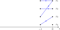
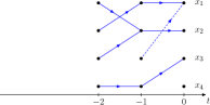
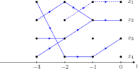
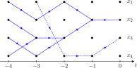
Figure 2: Coupling from the past

A sketch of the proof of Proposition 4.1 can be given using Figure 2. On the last of the four pictures, the Markov chain is run from time -4 onwards and its value is $x_{2}$ at time 0. If we had run the Markov chain from time $-\infty$ to 0, then the result would obviously still be $x_{2}$. But if we started from time $-\infty$, then the Markov chain would have reached equilibrium by time 0.

4.1.2 Infinite set of cells

Assume that the set of cells $E$ is infinite. Then a PCA defines a Markov chain on the infinite state space $X=\mathcal{A}^{E}$, so the above procedure is not effective anymore. However, it is possible to use the locality of the updating rule of a PCA to still define a perfect sampling procedure. (This observation already appears in [1].)

Let $P$ be an ergodic PCA and denote by $\pi$ its invariant distribution. In this context, a perfect sampling procedure is a random algorithm taking as input a finite subset $K$ of $E$ and returning a cylinder $x_{K}\in\mathcal{C}(K)$ with probability $\pi(x_{K})$.

To get such a procedure, we use the following fact: if the PCA is run from time $-k$ onwards, then to compute the content of the cells in $K$ at time 0, it is enough to consider the cells in the finite dependence cone of $K$. This is illustrated in Figure 3 for the set of cells $E=\mathbb{Z}$ and the neighborhood $V=\{-1,0,1\}$, with the choice $K=\{0\}$.

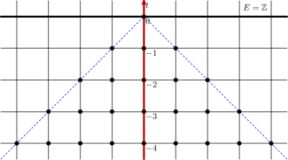
Figure 3: Dependence cone of a cell

Observe that the orientation has changed with respect to Figure 2 in order to be consistent with the convention of Figures 1 and 9 for space-time diagrams.

Let us define this more formally. Let $V$ be the neighborhood of the PCA. Given a subset $K$ of $E$, the dependence cone of $K$ is the family $(V_{-t}(K))_{t\geq 0}$ of subsets of $E$ defined recursively by $V_{0}(K)=K$ and $V_{-t}(K)=V+V_{-t+1}(K)$. Let $\phi:X\times[0,1]^{E}\rightarrow X$ be an update function, for instance the one defined according to (1). For a given subset $K$ of $E$, we denote $\phi_{-t}:\mathcal{A}^{V_{-t}(K)}\times[0,1]^{V_{-t}(K)}\rightarrow\mathcal{A}^{V_{-t+1}(K)}$ the corresponding restriction of $\phi$.

With these notations, the algorithm can be written as follows.

Data: An update function $\phi:X\times[0,1]^{E}\rightarrow X$ of a PCA. A family $(r^{-n}_{k})_{(k,n)\in E\times\mathbb{N}}$ of i.i.d. r.v. with uniform distribution in $[0,1]$. A finite subset $K$ of $E$.

begin

       $V_{0}(K)=K$ ;

       $t=1$ ;

       repeat

             $V_{-t}(K)=V+V_{-t+1}(K)$ ;

             $R_{-t}={\mathcal{A}}^{V_{-t}(K)}$ ;

             for $j=-t$ to $-1$ do

                  $R_{j+1}=\{\phi_{j}(x,(r^{j}_{i})_{i\in V_{j}(K)})\>;\>x\in R_{j}\}\subset\mathcal{A}^{V_{j+1}(K)}$

             end for

            $t=t+1$

      until $|R_{0}|=1$;

      return the unique element of $R_{0}$

end

Algorithm 2 Basic CFTP algorithm for an infinite set of cells

Next proposition is an easy extension of Proposition 4.1.

Proposition 4.2

If the procedure stops almost surely, then the PCA is ergodic and the output is distributed according to the marginal of the invariant measure.

4.2 Envelope probabilistic cellular automata (EPCA)

The CFTP algorithm is inefficient when the state space is large. This is the case for PCA: when $E$ is finite, the set $\mathcal{A}^{E}$ is very large, and when $E$ is infinite, it is the number of configurations living in the dependence cone described above which is very large. We cope with this difficulty by introducing the envelope PCA.

To begin with, let us assume that $P$ is a PCA on the alphabet $\mathcal{A}=\{0,1\}$ (as previously, the set of cells is denoted by $E$, the neighborhood by $V\subset E$, and the local function by $f$). The case of a general alphabet is treated in Section 4.5.

Definition of the EPCA.

Let us introduce a new alphabet:

$${\mathcal{B}}=\{{\mathbf{0}},{\mathbf{1}},{\mathbf{?}}\}.$$

A word on $\mathcal{B}$ is to be thought as a word on $\mathcal{A}$ in which the letters corresponding to some positions are not known, and are thus replaced by the symbol “${\mathbf{?}}$”. Formally we identify $\mathcal{B}$ with $2^{\mathcal{A}}-\emptyset$ as follows: ${\mathbf{0}}=\{0\}$, ${\mathbf{1}}=\{1\}$, and ${\mathbf{?}}=\{0,1\}$. So each letter of $\mathcal{B}$ is a set of possible letters of $\mathcal{A}$. With this interpretation, we view a word on $\mathcal{B}$ as a set of words on $\mathcal{A}$. For instance,

$$\mathbf{?}\mathbf{1}\mathbf{?}=\{010,011,110,111\}.$$

We will associate to the PCA $P$ a new PCA on the alphabet $\mathcal{B}$, that we call the envelope probabilistic cellular automaton of $P$.

Definition 4.3

The envelope probabilistic cellular automaton (EPCA) of $P$, is the PCA $\mbox{env}(P)$ of alphabet $\mathcal{B}$, defined on the set of cells $E$, with the same neighborhood $V$ as for $P$, and a local function $\mbox{env}(f):{\mathcal{B}}^{V}\rightarrow{\mathcal{M}}({\mathcal{B}})$ defined for each $y\in{\mathcal{B}}^{V}$ by

$$\mbox{env}(f)(y)({\mathbf{0}})=\min_{x\in\mathcal{A}^{V},\;x\in y}f(x)(0)$$

$$\mbox{env}(f)(y)({\mathbf{1}})=\min_{x\in\mathcal{A}^{V},\;x\in y}f(x)(1)$$

$$\mbox{env}(f)(y)({\mathbf{?}})=1-\min_{x\in\mathcal{A}^{V},\;x\in y}f(x)(0)-\min_{x\in\mathcal{A}^{V},\;x\in y}f(x)(1).$$

We point out that $\min_{x\in\mathcal{A}^{V},\;x\in y}f(x)(1)+\max_{x\in\mathcal{A}^{V},\;x\in y}f(x)(0)=1$, so that the last quantity $\mbox{env}(f)(y)({\mathbf{?}})$ is non-negative.

Moreover, $\mbox{env}(P)$ acts like $P$ on configurations which do not contain the letter “${\mathbf{?}}$”. More precisely,

$$\forall y\in{\mathcal{A}}^{V},\qquad\mbox{env}(f)(y)({\mathbf{0}})=f(y)(0),\quad\mbox{env}(f)(y)({\mathbf{1}})=f(y)(1),\quad\mbox{env}(f)(y)({\mathbf{?}})=0\>.$$ (3)

In particular, we get the following.

Proposition 4.4

If the EPCA $\mbox{env}(P)$ is ergodic then the PCA $P$ is ergodic.

Proof. According to (3), any invariant measure of $P$ corresponds to an invariant measure of $\mbox{env}(P)$. Therefore, if $P$ has several invariant measures, so does $\mbox{env}(P)$. Assume that $P$ has a unique invariant measure $\mu$ which is non-ergodic. Let $\mu_{0}$ be such that $\mu_{0}P^{n}$ does not converge to $\mu$. Then $\mu_{0}\ \mbox{env}(P)^{n}$ does not converge either, see (3). To summarize, we have proved that $P$ non-ergodic implies $\mbox{env}(P)$ non-ergodic. $\hfill\square$

The converse of Proposition 4.4 is not true and counter-examples will be given in Section 4.3.3.

Construction of an update function for the EPCA.

Let us define the update function

$$\tilde{\phi}:\mathcal{B}^{E}\times[0,1]^{E}\rightarrow\mathcal{B}^{E}$$

of the PCA $\mbox{env}(P)$, by:

$$\tilde{\phi}(y,r)_{k}=\left\{\begin{array}[]{l}{\mathbf{0}}\mbox{ if }0\leq r_{k}<\mbox{env}(f)((y_{k+v})_{v\in V})({\mathbf{0}})\\ {\mathbf{1}}\mbox{ if }1-\mbox{env}(f)((y_{k+v})_{v\in V})({\mathbf{1}})\leq r_{k}\leq 1\\ {\mathbf{?}}\mbox{ otherwise.}\\ \end{array}\right.$$ (4)

The value of $\tilde{\phi}(y,r)_{k}$ in function of $r_{k}$ can thus be represented as follows.

For a PCA of neighborhood $V=\{0,1\}$, we represent below the construction of the updates of the EPCA when the value of the neighborhood is $\mathbf{0}?$.

Let $\phi$ be the natural update function for the PCA $P$ defined as in (1). Observe that the function $\tilde{\phi}$ coincides with $\phi$ on configurations which do not contain the letter “${\mathbf{?}}$”. Furthermore, we have:

$$\forall r\in[0,1]^{E},\ \forall x\in\mathcal{A}^{E},\ \forall y\in\mathcal{B}^{E},\qquad x\in y\implies\phi(x,r)\in\tilde{\phi}(y,r)\>.$$ (5)

4.3 Perfect sampling using EPCA

We propose two perfect sampling algorithms, for a finite and for an infinite number of cells. We show that in both cases, the algorithm stops almost surely if and only if the EPCA is ergodic (Theorem 4.5). The ergodicity of the EPCA implies the ergodicity of the PCA but the converse is not true: we provide a counterexample for each case, finite and infinite (Section 4.3.3).We also give conditions of ergodicity of the EPCA (Prop. 4.6 and 4.7).

4.3.1 Algorithms

Finite set of cells.

The idea is to consider only one trajectory of the EPCA - the one that starts from the initial configuration ${\mathbf{?}}^{E}$ (coding the set of all configurations of the PCA). The algorithm stops when at time $0$, this trajectory hits the set $\mathcal{A}^{E}$.

Data: The pre-computed update function $\tilde{\phi}$. A family $(r^{-n}_{k})_{(k,n)\in E\times\mathbb{N}}$ of i.i.d. r.v. with uniform distribution in $[0,1]$.

begin

       $t=1$ ;

       repeat

             $c={\mathbf{?}}^{E}$ ;

             for $j=-t$ to $-1$ do

                  $c=\tilde{\phi}(c,(r^{j}_{i})_{i\in E})$

             end for

            $t=t+1$

      until $c\in\mathcal{A}^{E}$;

      return $c$

end

Algorithm 3 Perfect sampling using the EPCA for a finite set of cells

Infinite set of cells.

Once again, we consider only one trajectory of the EPCA.

Data: The pre-computed update function $\tilde{\phi}$. A family $(r^{-n}_{k})_{(k,n)\in E\times\mathbb{N}}$ of i.i.d. r.v. with uniform distribution in $[0,1]$. A finite subset $K$ of $E$.

begin

       $V_{0}(K)=K$ ;

       $t=1$ ;

       repeat

             $V_{-t}(K)=V+V_{-t+1}(K)$ ;

             $c={\mathbf{?}}^{V_{-t}(K)}$ ;

             for $j=-t$ to $-1$ do

                  $c=\tilde{\phi}_{j}(c,(r^{j}_{i})_{i\in V_{j}(K)})\in\mathcal{B}^{V_{j+1}(K)}$

             end for

            $t=t+1$

      until $c\in\mathcal{A}^{K}$;

      return $c$

end

Algorithm 4 Perfect sampling using the EPCA for an infinite set of cells

Theorem 4.5

Algorithm 3, resp. 4, stops almost surely if and only if the EPCA is ergodic. In that case, the output of the algorithm is distributed according to the unique invariant measure of the PCA.

Proof. The argument is the same in the finite and infinite cases. We give it for the finite case. Assume first that Algorithm 3 stops almost surely. By construction, it implies that for all $\mu_{0}$, the measure $\mu_{0}\ \mbox{env}(P)^{n}$ is asymptotically supported by $\mathcal{A}^{E}$. Therefore, we can strengthen the result in Proposition 4.4: the invariant measures of $\mbox{env}(P)$ coincide with the invariant measures of $P$. In that case, $\mbox{env}(P)$ is ergodic iff $P$ is ergodic. Using (5), the halting of Algorithm 3 implies the halting of Algorithm 1. Furthermore, if we use the same samples $(r^{-n}_{k})_{(k,n)\in E\times\mathbb{N}}$, Algorithms 3 and 1 will have the same output. According to Proposition 4.1, this output is distributed according to the unique invariant measure of $P$. In particular, $P$ is ergodic. So $\mbox{env}(P)$ is ergodic.

Assume now that the EPCA is ergodic. The unique invariant measure $\pi$ of $\mbox{env}(P)$ has to be supported by $\mathcal{A}^{E}$. Also, by ergodicity, we have $\delta_{\mathbf{?}^{E}}\ \mbox{env}(P)^{n}\stackrel{{\scriptstyle w}}{{\longrightarrow}}\pi$. This means precisely that the Algorithm 3 stops a.s. $\square$

4.3.2 Criteria of ergodicity for the EPCA

Finite set of cells.

In the next proposition, we give a necessary and sufficient condition for the EPCA to be ergodic. In particular, this condition is satisfied if the PCA has positive rates (see the Introduction).

Proposition 4.6

The EPCA $\mbox{env}(P)$ is ergodic if and only if $\mbox{env}(f)({\mathbf{?}}^{V})({\mathbf{?}})<1$. This condition can also be written as:

$$\min_{x\in\mathcal{A}^{V}}f(x)(0)+\min_{x\in\mathcal{A}^{V}}f(x)(1)>0.$$ (6)

Proof. If $\mbox{env}(f)({\mathbf{?}}^{V})({\mathbf{?}})=1$, then for almost any $r\in[0,1]^{E}$, we have $\tilde{\phi}({\mathbf{?}}^{E},r)={\mathbf{?}}^{E},$ so that at each step of the algorithm, the value of $c$ is ${\mathbf{?}}^{E}$ with probability 1.

Conversely, if we assume for example that $p=\min_{x\in{\mathcal{A}}^{V}}f(x)(0)>0$, then for any configuration $d\in\mathcal{B}^{E}$, the probability to have $\tilde{\phi}(x,r)={\mathbf{0}}^{E}$ is greater than $p^{|E|}$, so that the algorithm stops almost surely, and the expectation of the running time can be roughly bounded by $1/p^{|E|}$. $\square$

Infinite set of cells.

For an infinite set of cells the situation is more complex. The condition of Proposition 4.6 is not sufficient to ensure the ergodicity of the EPCA. A counter-example is given in Section 4.3.3. First, we propose a rough sufficient condition of convergence for Algorithm 4.

Proposition 4.7

Let $\alpha^{*}\in(0,1)$ be the critical probability of the percolation PCA with neighborhood $V$, see Examples 2.5 and 2.8. The EPCA $\mbox{env}(P)$ is ergodic if

$$\mbox{env}(f)(\mathbf{?}^{V})({\mathbf{?}})\ <\ \alpha^{*}$$ (7)

and non-ergodic if

$$\min_{x\in\mathcal{B}^{V}-\mathcal{A}^{V}}\mbox{env}(f)(x)({\mathbf{?}})\ >\ \alpha^{*}.$$ (8)

Proof. Recall that $\mathcal{B}=\{{\bf 0},{\bf 1},\mathbf{?}\}$. Define $\mathcal{C}=\left\{{\bf d},\mathbf{?}\right\}$, with ${\bf d}=\{{\bf 0},{\bf 1}\}$. A word over $\mathcal{C}$ is interpreted as a set of words over $\mathcal{B}$, for instance, ${\bf d}?=\{{\bf 0}\mathbf{?},{\bf 1}?\}$. The symbol d stands for determined letter, as opposed to ? which represents an unknown letter.

We define a new PCA $Q$ on the alphabet $\mathcal{C}$, with the same neighborhood $V$ as $P$ and $\mbox{env}(P)$, and with the transition function $g:{\mathcal{C}}^{V}\rightarrow{\mathcal{M}}({\mathcal{C}})$ defined by:

$$g({\bf d}^{V})=\delta_{{\bf d}},\quad\mbox{and}\quad\forall u\in\mathcal{C}^{V}-\{{\bf d}^{V}\},\quad g(u)=\alpha\delta_{\mathbf{?}}+(1-\alpha)\delta_{{\bf d}}\>,$$

for $\alpha=\max_{x\in\mathcal{B}^{V}}\mbox{env}(f)(x)({\mathbf{?}})=\mbox{env}(f)(\mathbf{?}^{V})({\mathbf{?}})$.

Observe that $\delta_{{\bf d}^{E}}$ is an invariant measure of $Q$. Recall that $\tilde{\phi}$ is an update function of $\mbox{env}(P)$, see (4). Given the way $Q$ is defined, we can construct an update function $\phi_{Q}$ of $Q$ such that

$$\forall x\in\mathcal{B}^{E},\forall y\in\mathcal{C}^{E},\forall r\in[0,1]^{E},\qquad x\in y\implies\tilde{\phi}(x,r)\in\phi_{Q}(y,r)\>.$$ (9)

In particular, assume that $Q$ is ergodic. Then $\delta_{\mathbf{?}^{E}}\ Q^{n}\stackrel{{\scriptstyle w}}{{\longrightarrow}}\delta_{{\bf d}^{E}}$. Using (9), it implies that Algorithm 4 stops almost surely, and $\mbox{env}(P)$ is ergodic according to Theorem 4.5. To summarize, the ergodicity of $Q$ implies the ergodicity of $\mbox{env}(P)$.

Observe that the PCA $Q$ is a percolation PCA as defined in Example 2.5 (here, d plays the role of 0 and $\mathbf{?}$ plays the role of 1). Let $\alpha^{*}\in(0,1)$ be the critical probability of the percolation PCA with neighborhood $V$, see Example 2.8. For $\alpha<\alpha^{*}$, the percolation PCA $Q$ is ergodic. This completes the proof of (7).

Define a PCA $R$ on the alphabet $\mathcal{C}$, with neighborhood $V$, and with the transition function:

$$h({\bf d}^{V})=\delta_{{\bf d}},\quad\mbox{and}\quad\forall u\in\mathcal{C}^{V}-\{{\bf d}^{V}\},\quad h(u)=\beta\delta_{\mathbf{?}}+(1-\beta)\delta_{{\bf d}}\>,$$

for $\beta=\min_{x\in\mathcal{B}^{V}-\mathcal{A}^{V}}\mbox{env}(f)(x)({\mathbf{?}})$. Given the way $R$ is defined, we can construct an update function $\phi_{R}$ of $R$ such that

$$\forall x\in\mathcal{B}^{E},\forall y\in\mathcal{C}^{E},\forall r\in[0,1]^{E},\forall k\in E,\qquad[x\in y,\ \phi_{R}(y,r)_{k}=\mathbf{?}]\implies\tilde{\phi}(x,r)_{k}=\mathbf{?}\>.$$

Therefore, the ergodicity of $env(P)$ implies the ergodicity of $R$. Equivalently, the non-ergodicity of $R$ implies the non-ergodicity of $env(P)$. Observe that the PCA $R$ is a percolation PCA. Therefore, for $\beta>\alpha^{*}$, the percolation PCA $R$ is non-ergodic. This completes the proof of (8).

$\square$

4.3.3 Counter-examples

Recall Proposition 4.4: [ EPCA ergodic ] $\implies$ [ PCA ergodic ]. We now show that the converse is not true.

Example 4.8

Consider the PCA with alphabet $\mathcal{A}=\{0,1\}$, neighborhood $V=\{-1,0,1\}$, set of cells $E=\mathbb{Z}/n\mathbb{Z}$, and transition function

$$f(x,y,z)=\begin{cases}\delta_{1-y}&\mbox{if }xyz\in\{101,010\}\\ \alpha\delta_{y}+(1-\alpha)\delta_{1-y}&\mbox{otherwise}\>,\end{cases}$$

for a parameter $\alpha\in(0,1)$. This is the PCA Majority studied in Section 5. For $n$ odd, we prove in Proposition 5.1 that the PCA is ergodic. However the associated EPCA satisfies $\mbox{env}(f)(???)=\delta_{?}$. According to Proposition 4.6, the EPCA is not ergodic.

Example 4.9

Consider the PCA of Example 2.4. This PCA has positive rates, in particular, it satisfies (6). So the EPCA is ergodic on a finite set of cells. Now let the set of cells be $\mathbb{Z}$. The PCA is ergodic for $\varepsilon\in(0,1)$, see Example 2.7. Consider the associated EPCA $\mbox{env}(P)$. Assume for instance that $\varepsilon\in(0,1/2)$. We have

$$\mbox{env}(f)(u)=\begin{cases}f(u)&\mbox{if }u\in\{\mathbf{0},\mathbf{1}\}^{V}\\ \varepsilon\delta_{{\bf 0}}+\varepsilon\delta_{{\bf 1}}+(1-2\varepsilon)\delta_{\mathbf{?}}&\mbox{otherwise}\>.\end{cases}$$

By applying Proposition 4.7, $\mbox{env}(P)$ is non-ergodic if $1-2\varepsilon>\alpha^{*}.$

4.4 Decay of correlations

In what follows, the set of cells is $E=\mathbb{Z}^{d},\ d\geq 1$. It is easy to prove that the invariant measure of an ergodic PCA is shift-invariant. Using the coupling from the past tool, we give conditions for the invariant measure of an ergodic PCA to be shift-mixing.

Definition 4.10

A measure $\mu$ on $X={\cal A}^{\mathbb{Z}^{d}}$ is shift-mixing if for any non-trivial translation shift $\tau$ of $\mathbb{Z}^{d}$, and for any cylinders $U,V$ of $X$,

$$\lim_{n\rightarrow+\infty}\mu(U\cap\tau^{-n}(V))=\mu(U)\mu(V).$$ (10)

The proof of the following proposition is inspired from the proof of the validity of the coupling from the past method (see [24] or [16]).

Figure 4: Illustration of the proof of Proposition 4.11

Proposition 4.11

If Algorithm 2 stops almost surely, then the unique invariant measure of the PCA is shift-mixing. It is in particular the case under condition (7).

Proof. Assume that $P$ is an ergodic PCA, and denote by $\pi$ its unique invariant measure. Let $K$ and $L$ be two finite subsets of $E$, and denote by $x_{K}$ and $y_{L}$ some cylinders corresponding to these subsets. Since the perfect sampling algorithm stops almost surely, for each $\varepsilon>0$, there exists an integer $t_{\varepsilon}$ such that with probability greater than $1-\varepsilon$, the algorithm stops before reaching the time $-t_{\varepsilon}$ when it is run for the set of cells $K$ or for the set of cells $L$. If $n\in\mathbb{N}^{d}$ is large enough, we have: $V_{-t_{\varepsilon}}(K)\cap V_{-t_{\varepsilon}}(\tau^{-n}(L))=\varnothing$.

Let $Z$ be the output of the algorithm if it is asked to sample the marginals of $\pi$ corresponding to the cells of $K\cup\tau^{-n}(L)$.

Imagine running the PCA from time $-t_{\varepsilon}$ and set of cells $V_{-t_{\varepsilon}}(K)\cup V_{-t_{\varepsilon}}(\tau^{-n}(L))$ up to time $0$, using the same update variables as the ones used to get $Z$. Choose the initial condition at time $-t_{\varepsilon}$ as follows: independently on $V_{-t_{\varepsilon}}(K)$ and $V_{-t_{\varepsilon}}(\tau^{-n}(L))$, and according to the relevant marginals of $\pi$. Let $X$, resp. $Y$, be the output at time 0 on the set of cells $K$, resp. $\tau^{-n}(L)$. Observe that $X$ and $Y$ are distributed according to the marginals of $\pi$. Furthermore, $X$ and $Y$ are independent since the dependence cones of $K$ and $\tau^{-n}(L)$ originating at time $-t_{\varepsilon}$ are disjoint. We therefore get

$$\pi(x_{K}\cap\tau^{-n}(y_{L}))-\pi(x_{K})\pi(y_{L}) ={\mathbb{P}}(Z_{K}=x_{K},Z_{\tau^{-n}(L)}=y_{L})-{\mathbb{P}}(X=x_{K}){\mathbb{P}}(Y=y_{L})$$

$$={\mathbb{P}}(Z_{K}=x_{K},Z_{\tau^{-n}(L)}=y_{L})-{\mathbb{P}}(X=x_{K},Y=y_{L})$$

$$\leq{\mathbb{P}}((Z_{K},Z_{\tau^{-n}(L)})=(x_{K},y_{L})\mbox{ and }(X,Y)\not=(x_{K},y_{L}))$$

$$\leq{\mathbb{P}}((Z_{K},Z_{\tau^{-n}(L)})\not=(X,Y))\ \leq\ 2\varepsilon\>.$$

In the same way, we get $\pi(x_{K})\pi(y_{L})-\pi(x_{K}\cap\tau^{-n}(y_{L}))\leq 2\varepsilon$. It completes the proof. $\square$

In Proposition 4.11, the coupling from the past method is not used as a sampling tool but as a way to get theoretical results. Knowing if there exists an ergodic PCA having an invariant measure which is not shift-mixing is an open question (see [6] for details).

4.5 Extensions

In a PCA, the dynamic is homogeneous in space. It is possible to get rid of this characteristic by defining non-homogeneous PCA, for which the neighborhood and the transition function depend on the position of the cell. The definition below is to be compared with Definition 2.1. The configuration space $X=\mathcal{A}^{E}$ is unchanged.

Definition 4.12

For each $k\in E$, denote by $V_{k}\subset E$ the (finite) neighborhood of the cell $k$, and by $f_{k}:\mathcal{A}^{V_{k}}\rightarrow\mathcal{M}(\mathcal{A})$ the transition function associated to $k$. Set $\mathcal{V}(K)=\cup_{k\in K}V_{k}$. The non-homogeneous PCA (NH-PCA) of transition functions $(f_{k})_{k\in E}$ is the application $P:\mathcal{M}(X)\rightarrow\mathcal{M}(X),\ \mu\mapsto\mu P$, defined on cylinders by

$$\mu P(y_{K})=\sum_{x_{\mathcal{V}(K)}\in\mathcal{C}(\mathcal{V}(K))}\mu(x_{\mathcal{V}(K)})\prod_{k\in K}f_{k}((x_{v})_{v\in V_{k}})(y_{k})\>.$$

Observe that it is not necessary for $E$ to be equipped with a semigroup structure anymore. We use this below to define the finite restriction of a PCA.

It is quite straightforward to adapt the coupling from the past algorithms to NH-PCA. More precisely, given a NH-PCA, we define the associated NH-EPCA by considering Definition 4.3 and replacing $V$ and $\mbox{env}(f)$ by $V_{k}$ and $\mbox{env}(f)_{k}$ for each $k\in E$. The algorithms of Section 4.1 and 4.3.1 are then unchanged, and Proposition 4.4 and Theorem 4.5 still hold in the non-homogeneous setting.

In Section 5, we study the PCA Majority by approximating it by a sequence of NH-PCA. Let us explain the construction in a general setting.

Let $P$ be a PCA on the infinite set of cells $E$, with neighborhood $V$ and transition function $f:\mathcal{A}^{V}\rightarrow\mathcal{M}(\mathcal{A})$. Let $D$ be a finite subset of $E$. Define

$$\overline{V}(D)=\{u\in E\mid\exists x\in D,\exists v\in V\cup\{0\},\ u=x+v\},\quad B(D)=\overline{V}(D)-D\>.$$

The set $B(D)$ is the boundary of the domain $D$. Fix a probability measure $\nu$ on $\mathcal{A}$. The restriction of $P$ associated with $\nu$ and $D$ is the NH-PCA $P(\nu,D)$ with set of cells $\overline{V}(D)$ and neighborhoods:

$$\forall u\in D,\ V_{u}=\{u\}+V,\qquad\forall u\in B(D),\ V_{u}=\varnothing\>;$$

and transition functions:

$$\forall u\in D,\ f_{u}=f,\qquad\forall u\in B(D),\ f_{u}(\cdot)=\nu\>.$$

In words, the boundary cells are i.i.d. of law $\nu$ and the cells of $D$ are updated according to $P$.

If $\mu$ is a probability measure on $\mathcal{A}^{S}$, where $S$ is a finite subset of $E$, we define its extension $\tilde{\mu}$ on $\mathcal{A}^{E}$ by setting, for a fixed letter $a\in\mathcal{A}$:

$$\forall x\in\mathcal{A}^{E},\ \tilde{\mu}(x)=\begin{cases}\mu((x_{k})_{k\in S})&\mbox{if }\forall i\in E-S,\ x_{i}=a\\ 0&\mbox{ otherwise.}\end{cases}$$

Lemma 4.13

Let $(D_{i})_{i\in\mathbb{N}}$ be an increasing sequence of finite domains $D_{i}\subset E$ such that $\cup_{i\in\mathbb{N}}D_{i}=E$. Let $(\nu_{i})_{i\in\mathbb{N}}$ be a sequence of probability measures on $\mathcal{A}$. For each $i$, let $\mu_{i}$ be an invariant measure of $P(\nu_{i},D_{i})$. Any accumulation point of the sequence $(\tilde{\mu}_{i})_{i\in\mathbb{N}}$ is an invariant measure of the original PCA $P$ defined on $E$.

Proof. Upon extracting a subsequence, we may assume that $(\tilde{\mu}_{j})_{j\in\mathbb{N}}$ converges to $\tilde{\mu}\in\mathcal{M}(X)$. We need to prove that for any cylinder $y_{K}\in\mathcal{C}(K),$ we have $\tilde{\mu}P(y_{K})=\tilde{\mu}(y_{K})$.

By definition, $\mu_{j}P(\nu_{j},D_{j})=\mu_{j}$. Let the subset $K$ of $E$ and the cylinder $y_{K}\in\mathcal{C}(K)$ be fixed. If $j$ is large enough, we have $K\subset D_{j}$ and $\overline{V}(K)\subset D_{j}$. So that $\mu_{j}(y_{K})=\tilde{\mu}_{j}(y_{K})$ and $P(\nu_{j},D_{j})$ and $P$ coincide on $K$. We deduce that $\tilde{\mu}_{j}P(y_{K})=\tilde{\mu}_{j}(y_{K})$. By taking the limit on both sides, we get $\tilde{\mu}P(y_{K})=\tilde{\mu}(y_{K})$. $\hfill\square$

Alphabet with more than two elements

The EPCA and the associated algorithms have been defined on a two letters alphabet. It is possible to extend the approach to a general finite alphabet.

Let $\mathcal{A}$ be the finite alphabet. Let $P$ be a PCA with set of cells $E$, neighborhood $V$, and transition function $f:\mathcal{A}^{V}\rightarrow\mathcal{M}(\mathcal{A})$.

Consider the alphabet $\mathcal{B}=2^{\mathcal{A}}-\{\varnothing\}$, that is, the set of non-empty subsets of $\mathcal{A}$. A word over $\mathcal{B}$ is viewed as a set of words over $\mathcal{A}$.

The EPCA $\mbox{env}(P)$ associated with $P$ is the PCA on the alphabet $\mathcal{B}$ with neighborhood $V$ and transition function $\mbox{env}(f)$ defined by:

$$\forall v\in\mathcal{B}^{V},\ \forall y\in\mathcal{B},\qquad\mbox{env}(f)(v)(y)=\sum_{x\subset y}(-1)^{|y|-|x|}\min_{u\in v}f(u)(x)\>.$$

For instance, we have: $\mbox{env}(f)(v)(\{0,1,2\})=\alpha_{0,1,2}-\alpha_{0,1}-\alpha_{1,2}-\alpha_{0,2}+\alpha_{0}+\alpha_{1}+\alpha_{2}$ with $\alpha_{S}=\min_{u\in v}f(u)(\{S\})$.

The algorithms of Section 4.3 are unchanged. Observe however that the construction of an update function is not as natural as in the two-letters alphabet case.

5 The majority PCA: a case study

The Majority PCA is one of the simplest examples of PCA whose behaviour is not well understood. Therefore, it provides a good case study for the sampling algorithms of Section 4.

5.1 Definition of the majority PCA

Given $0<\alpha<1$, the PCA Majority$(\alpha)$, or simply Majority, is the PCA on the alphabet $\mathcal{A}=\{0,1\}$, with set of cells $E=\mathbb{Z}$ (or $\mathbb{Z}/n\mathbb{Z}$), neighborhood $V=\{-1,0,1\}$, and transition function

$$f(x,y,z)=\alpha\,\delta_{\mbox{maj}(x,y,z)}+(1-\alpha)\,\delta_{1-y}\>,$$

where $\mbox{maj}:\mathcal{A}^{3}\rightarrow\mathcal{A}$ is the majority function: the value of $\mbox{maj}(x,y,z)$ is $0$, resp. 1, if there are two or three $0$’s, resp $1$’s, in the sequence $x,y,z$. The transition function of PCA Majority$(\alpha)$ can thus be represented as in Figure 5. It consists in choosing independently for each cell to apply the elementary rule 232 (with probability $\alpha$) or to flip the value of the cell.

The PCA Minority$(\alpha)$ has also been studied (see [26]). It is defined by the transition function $g(x,y,z)=f(1-x,1-y,1-z)$.

Figure 5: The transition function of the PCA Majority

Let $x=(01)^{\mathbb{Z}}\in\{0,1\}^{\mathbb{Z}}$ be defined by: $\forall n\in\mathbb{Z}$, $x_{2n}=0,\ x_{2n+1}=1$. The configuration $(10)^{\mathbb{Z}}$ is defined similarly. Consider the probability measure

$$\mu=(\delta_{(01)^{\mathbb{Z}}}+\delta_{(10)^{\mathbb{Z}}})/2\>.$$ (11)

Clearly $\mu$ is an invariant measure for the PCA Majority. The question is whether there exists other invariant measures.

To get some other insight on the question of invariant measures, consider the PCA Majority on the set of cells $\mathbb{Z}_{n}={\mathbb{Z}/n\mathbb{Z}}$. This PCA has two completely different behaviors depending on the parity of $n$.

Proposition 5.1

Consider the Markov chain on the state space $\{0,1\}^{\mathbb{Z}_{n}}$ which is induced by the Majority PCA. The Markov chain has a unique invariant measure $\nu$. If $n$ is even then $\nu=(\delta_{(01)^{n/2}}+\delta_{(10)^{n/2}})/2$; if $n$ is odd then $\nu$ is supported by $\{0,1\}^{\mathbb{Z}_{n}}$.

Proof. Let $Q$ be the transition matrix of the Markov chain. We are going to prove the following. If $n$ is odd, then $Q$ is irreducible and aperiodic. If $n$ is even, the graph of $Q$ has a unique terminal component consisting of the two points $(01)^{n/2}=0101\ldots 01$ and $(10)^{n/2}=1010\ldots 10$.

Assume first that $n$ is odd. From the configurations $0^{n}=0\ldots 0$ or $1^{n}=1\ldots 1$, we can go to any configuration in one step. So, we only need to prove that from a given configuration, say $c\in\{0,1\}^{\mathbb{Z}_{n}}$, it is possible to reach $0^{n}$ or $1^{n}$. We assume that $c$ is neither $0^{n}$ nor $1^{n}$, and we consider the length $L$ of the longest subsequence of identical bits in $c$. Since $n$ is odd, there are at least two consecutive $0$’s or two consecutive $1$’s. So, we have $L\geq 2$. Say that we have the pattern $10^{L}1$ in $c$. With probability $(1-\alpha)^{2}\alpha^{L}$, the update of the corresponding cells will be: flip, majority, majority, …, majority, flip. Thus after one step, we can obtain configurations with the pattern $0^{L+2}$ (or $0^{n}$ if $L=n-1$). By iterating, we see that after at most $n/2$ steps, we can reach configuration $0^{n}$ or $1^{n}$.

Assume now that $n$ is even. Clearly

$$\delta_{(01)^{n/2}}Q=\delta_{(10)^{n/2}},\qquad\delta_{(10)^{n/2}}Q=\delta_{(01)^{n/2}}\>.$$

Thus, $\{(01)^{n/2},(10)^{n/2}\}$ is a terminal component of the graph of $Q$. Consider $c\in\{0,1\}^{\mathbb{Z}_{n}}-\{(01)^{n/2},(10)^{n/2}\}$. Then $c$ has at least two consecutive $0$’s or $1$’s. We can use the same argument as for $n$ odd, to show that we can reach $0^{n}$ or $1^{n}$ in at most $n/2$ steps. We conclude by observing that $(01)^{n/2}$ can be reached from $0^{n}$ or $1^{n}$ in one step. $\hfill\square$

Let us come back to the PCA Majority on $\mathbb{Z}$. The invariant measure $\mu$ in (11) can be viewed as the “limit” over $n$ of the invariant measures of the PCA on $\mathbb{Z}_{2n}$. What about the “limits” of the invariant measures of the PCA on $\mathbb{Z}_{2n+1}$ ? Do they define other invariant measures for the PCA on $\mathbb{Z}$ ?

One of the motivations of our work on perfect sampling algorithms for PCA was to test the following conjecture, which is inspired by the observations made in [25] and [26] on a PCA equivalent to Majority. This conjecture concerns the existence of a “phase transition” phenomenon for the PCA Majority.

Conjecture 5.2

There exists $\alpha_{c}\in(0,1)$ such that Majority$(\alpha)$ has a unique invariant measure if $\alpha<\alpha_{c}$, and several invariant measures if $\alpha>\alpha_{c}$.

In the next subsection, we give some rigorous (but partial) results about the invariant measures of Majority($\alpha$). We first introduce a related PCA and use it to prove that if $\alpha$ is large enough, Majority$(\alpha)$ has indeed non-trivial invariant measures; we then present a dual model that could be used to have some information for small values of $\alpha$.

The last subsection is devoted to the experimental study of Majority$(\alpha)$ using the perfect sampling tools developed in the previous section.

5.2 Theoretical study

5.2.1 A related model: the “flip-if-not-all-equal” PCA

Let us define as in [25], the PCA FINAE($\alpha$) of neighborhood $V=\{-1,0,1\}$ and transition function $g:\{0,1\}^{V}\rightarrow\mathcal{M}(\{0,1\})$ given by

$$g(x,y,z)=\alpha\delta_{\mbox{flip-if-not-all-equal}(x,y,z)}+(1-\alpha)\delta_{y}\>,$$

where the function flip-if-not-all-equal (FINAE), corresponding to the elementary cellular automaton 178, is defined by

$$\mbox{flip-if-not-all-equal}(x,y,z)=\begin{cases}y&\mbox{if }x=y=z\\ 1-y&\mbox{otherwise.}\end{cases}\>$$

Clearly, $\delta_{0^{\mathbb{Z}}}$ and $\delta_{1^{\mathbb{Z}}}$ are invariant measures of the PCA.

Let us define $\mbox{flip-odd}:\{0,1\}^{\mathbb{Z}}\rightarrow\{0,1\}^{\mathbb{Z}}$ and $\mbox{flip-even}:\{0,1\}^{\mathbb{Z}}\rightarrow\{0,1\}^{\mathbb{Z}}$ by, for $x=(x_{i})_{i\in\mathbb{Z}}$,

$$\mbox{flip-odd}(x)_{i}=\begin{cases}x_{i}&\mbox{if }i\mbox{ is even}\\ 1-x_{i}&\mbox{if }i\mbox{ is odd}\end{cases},\qquad\mbox{flip-even}(x)_{i}=\begin{cases}1-x_{i}&\mbox{if }i\mbox{ is even}\\ x_{i}&\mbox{if }i\mbox{ is odd}\end{cases}\>.$$

If we extend flip-odd and flip-even to mappings on $\mathcal{M}(\{0,1\}^{\mathbb{Z}})$, we have

$$\mbox{Majority}(\alpha)=\mbox{flip-odd}\circ\mbox{FINAE}(\alpha)\circ\mbox{flip-even}\>.$$

This equality can be checked on the local functions of the PCA Majority$(\alpha)$ and FINAE$(\alpha)$. One thus obtains that if $\pi$ is an invariant measure for FINAE$(\alpha)$, then

$$(\mbox{flip-odd}(\pi)+\mbox{flip-even}(\pi))/2$$

is an invariant measure for Majority$(\alpha)$. The invariant measures $\delta_{0^{\mathbb{Z}}}$ and $\delta_{1^{\mathbb{Z}}}$ of FINAE$(\alpha)$ correspond to the invariant measure $\mu$ in (11) for Majority$(\alpha)$, and the existence of a non-trivial invariant measure for FINAE$(\alpha)$ corresponds to the existence of a second invariant measure for Majority$(\alpha)$.

5.2.2 Validity of the conjecture for large values of $\alpha$

The partial result of Proposition 5.3 relies on ideas from Regnault [25].

Proposition 5.3

Let $p_{c}$ be the percolation threshold of directed bond-percolation in $\mathbb{N}^{2}$. If $\alpha\geq\sqrt[3]{1-(1-p_{c})^{4}}$, then Majority$(\alpha)$ has several invariant measures (resp. FINAE$(\alpha)$ has other invariant measures than the combinations of $\delta_{0^{\mathbb{Z}}}$ and $\delta_{1^{\mathbb{Z}}}$). It is in particular the case if $\alpha\geq 0.996$.

Proof. It is known that $0.6298\leq p_{c}\leq 2/3$, see for instance Grimmett [14]. This provides the bound $\sqrt[3]{1-(1-p_{c})^{4}}\leq 0.996$.

Let us consider the directed graph $G=(N,A)$ such that the set of nodes is $N=2\mathbb{Z}\times 2\mathbb{N}\cup(2\mathbb{Z}+1)\times(2\mathbb{N}+1)$ and for each $(i,j)\in N$, there is an arc (oriented bond) from $(i,j)$ to $(i-1,j+1)$ and one from $(i,j)$ to $(i+1,j+1)$.

Figure 6: The graph $G$

Let $S$ be some subset of $2\mathbb{Z}\times\{0\}$ called the source. The oriented bond-percolation on $G$ of parameter $p$ and source $S$ is defined as follows: each node is open with probability $p$ and closed with probability $1-p$, independently of the others, and a node of $N$ is said to be wet if there is an open path joining it from some node of $S$.

We say that the space-time diagram $(x^{t}_{k})_{k\in\mathbb{Z},t\in\mathbb{N}}$ of FINAE$(\alpha)$ and the percolation model satisfy the correspondence criterion at time $t$ if for each wet cell $(k,t)$ of height $t$, we have $x_{k}^{t}\not=x_{k+1}^{t}$ or $x_{k}^{t}\not=x_{k-1}^{t}$.

For values of $(\alpha,p)$ satisfying $\alpha\geq\sqrt[3]{1-(1-p)^{4}}$, Regnault is able to construct a coupling between FINAE$(\alpha)$ and the percolation model such that if the correspondence criterion is true at time $t$, it is still true at time $t+1$. Let us take for the initial configuration of FINAE$(\alpha)$ the configuration $x^{0}$ defined by $x^{0}_{k}=1$ if $k$ is odd and $x^{0}_{k}=0$ if $n$ is even. We also choose $S=2\mathbb{Z}\times\{0\}$ for the percolation model. The correspondence criterion is true at time $0$. By the coupling described in [25], the criterion is true at all time.

Consider the percolation model and the probability ${\mathbb{P}}((0,2t)\mbox{ is wet})$. It is known (see for example [14]) that if $p$ is strictly greater than a certain critical value $p_{c}$, this probability, which decreases with $t$, does not tend to $0$. Thus, for $p>p_{c}$, there exists $\eta_{p}>0$ such that ${\mathbb{P}}((0,2t)\mbox{ is wet})>\eta_{p}$ for all $t\in\mathbb{N}$. By construction of the coupling, we obtain ${\mathbb{P}}(x_{0}^{2t}\not=x_{1}^{2t}\mbox{ or }x_{0}^{2t}\not=x_{-1}^{2t})\geq\eta_{p}$ for all $t\in\mathbb{N}$. This proves that for $\alpha\geq\sqrt[3]{1-(1-p_{c})^{4}}$, the PCA FINAE$(\alpha)$ has at least one invariant measure which is not in the convex hull of the Dirac masses at the configurations “all zeroes” and “all ones” (take any accumulation point of the Cesàro sums obtained from the sequence obtained from the iterated of $\delta_{x^{0}}$ by FINAE). This result can be translated to the PCA Majority. $\hfill\square$

5.2.3 A duality result with the double branching annihilating random walk

The aim of this subsection is to prove a duality result between FINAE$(\alpha)$ and a double branching annihilating random walk (DBARW). The connection between these two models is interesting in itself and could provide a new way to study the PCA Majority$(\alpha)$ for small values of $\alpha$. A similar duality result was already obtained for interacting particle systems (see [7]), and the behavior of the DBARW is very well understood in continuous time (see [27]), but its study appears to be more difficult in discrete time.

We now assume that $\alpha\leq 2/3$ (in particular, Proposition 5.3 does not apply).

Let us define a process $(x_{k}^{t})_{k\in\mathbb{Z},t\in\mathbb{N}}$ in the following way. For each $(k,t)\in\mathbb{Z}\times\mathbb{N}$, we first choose independently to do one (and only one) of the following:

1. with probability $\alpha/2$, draw an arc from $(k-1,t)$ to $(k,t+1)$,

2. with probability $\alpha/2$, draw an arc from $(k+1,t)$ to $(k,t+1)$,

3. with probability $\alpha/2$, draw an arc from $(k-1,t)$ to $(k,t+1)$, an arc from $(k,t)$ to $(k,t+1)$, and an arc from $(k+1,t)$ to $(k,t+1)$,

4. with probability $1-3\alpha/2$, draw an arc from $(k,t)$ to $(k,t+1)$.

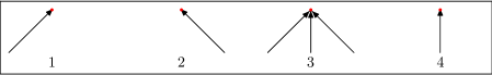
Figure 7: Construction of the graph $G_{1}$

We thus obtain a directed graph $G_{1}$, that we will use to label each node of $\mathbb{Z}\times\mathbb{N}$ with a letter of $\{0,1\}$. The nodes of $\mathbb{Z}\times\{0\}$ are labeled according to the wanted initial configuration $x^{0}$. A node labeled by a $1$ will be interpreted as being occupied. A node $(k,t)\in\mathbb{Z}\times\mathbb{N}$ is then labeled by a $1$ if and only if there is an odd number of paths leading to this node from an occupied node of $\mathbb{Z}\times\{0\}$. This define a random field $(x_{k}^{t})_{k\in\mathbb{Z},t\in\mathbb{N}}$ representing the labels of the nodes.

We claim that this field has the same distribution as a space-time diagram of FINAE$(\alpha)$ starting from $x^{0}$. Indeed, the value $x_{k}^{t+1}$ is equal to $x_{k-1}^{t}$ with probability $\alpha/2$, to $x_{k+1}^{t}$ with probability $\alpha/2$, to $x_{k-1}^{t}+x_{k}^{t}+x_{k+1}^{t}\mathop{\rm mod}\nolimits 2$ with probability $\alpha/2$ and to $x_{k}^{t}$ with probability $1-3\alpha/2$. And one can check for each value $(x,y,z)\in\{0,1\}^{3}$ that these probabilities coincide with the ones obtained with the local function flip-if-not-all-equal. For example, if $(x_{k-1}^{t},x_{k}^{t},x_{k+1}^{t})=(0,0,1)$, the value of $x_{k}^{t+1}$ will be $1$ if and only if case $2$ or case $3$ occurs, and they have together a probability $\alpha/2+\alpha/2=\alpha$. If $(x_{k-1}^{t},x_{k}^{t},x_{k+1}^{t})=(0,1,0)$, we will have $x_{k}^{t+1}=1$ if and only if case $3$ or case $4$ occurs, which has a probability $\alpha/2+(1-3\alpha/2)=1-\alpha$. And if $(x_{k-1}^{t},x_{k}^{t},x_{k+1}^{t})=(0,0,0)$ (resp. $(1,1,1)$), we will get a $0$ (resp. a $1$) in all cases.

We now consider the process $(y_{k}^{t})_{k\in\mathbb{Z},t\in\mathbb{N}}$ obtained from $(x_{k}^{t})_{k\in\mathbb{Z},t\in\mathbb{N}}$ by reversing time. Formally, for each $(k,t)\in\mathbb{Z}\times\mathbb{N}$, we first choose independently to do one (and only one) of the following things:

1. with probability $\alpha/2$, draw an arc from $(k,t)$ to $(k-1,t+1)$;

2. with probability $\alpha/2$, draw an arc from $(k,t)$ to $(k+1,t+1)$;

3. with probability $\alpha/2$, draw an arc from $(k,t)$ to $(k-1,t+1)$, an arc from $(k,t)$ to $(k,t+1)$, and an arc from $(k,t)$ to $(k+1,t+1)$;

4. with probability $1-3\alpha/2$, draw an arc from $(k,t)$ to $(k,t+1)$.

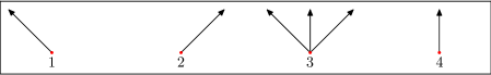
Figure 8: Construction of the graph $G_{2}$

We thus obtain again a directed graph $G_{2}$, that we will use to label each node of $\mathbb{Z}\times\mathbb{N}$ with a letter of $\{0,1\}$. The nodes of $\mathbb{Z}\times\{0\}$ are labeled according to the wanted initial configuration $y^{0}$. A node labeled by a $1$ will be interpreted as being occupied. A node $(k,t)\in\mathbb{Z}\times\mathbb{N}$ is then labeled by a $1$ if and only if there is an odd number of paths leading to this node from an occupied node of $\mathbb{Z}\times\{0\}$. This define a random field $(y_{k}^{t})_{k\in\mathbb{Z},t\in\mathbb{N}}$ representing the labels of the nodes.

We claim that this field has the same distribution as the double branching annihilating random walk c that we now define.

At time $0$, a particles is placed on each cell $k$ of $\mathbb{Z}$ such that $y^{0}_{k}=1$, and at each step of time, every particle chooses independently of the others do one (and only one) of the following things:

1. with probability $\alpha/2$, move from node $k$ to $k-1$;

2. with probability $\alpha/2$, move from node $k$ to $k+1$;

3. with probability $\alpha/2$, stay at node $k$ and create two new particles at nodes $k-1$ and $k+1$;

4. with probability $1-3\alpha/2$, stay at node $k$.

If after these choices, there is an even number of particles at a node, then all these particles annihilate. If there is an odd number of them, only one particle survives. We set $w_{k}^{t}=1$ if and only if at time $t$, there is a particle at node $k$.

To summarize, we have the following relations:

$$\mbox{ FINAE }\sim(x_{k}^{t})_{k\in\mathbb{Z},t\in\mathbb{N}}\stackrel{{\scriptstyle\mbox{ time-reversal }}}{{\longleftrightarrow}}(y_{k}^{t})_{k\in\mathbb{Z},t\in\mathbb{N}}\sim\mbox{ DBARW}$$

The processes $(x_{k}^{t})_{k\in\mathbb{Z},t\in\mathbb{N}}$ and $(y^{t}_{k})_{k\in\mathbb{Z},t\in\mathbb{N}}$ are obtained one from another by reversing time. This can be used to get nontrivial information for FINAE. For instance, if $A$ represents the set of occupied nodes at time $0$ for $x$, that is to say $x^{0}={1}_{A}$, we have the following duality relation:

$${\mathbb{P}}^{\;x^{0}={1}_{A}}(x_{k}^{t}\not=x_{l}^{t})={\mathbb{P}}^{\;x^{0}={1}_{A}}(x_{k}^{t}+x_{l}^{t}=1)$$

$$={\mathbb{P}}(\mbox{the total number of paths in }G_{1}\mbox{ leading from }A\times\{0\}\mbox{ to }(k,t)\mbox{ or }(l,t)\mbox{ is odd})$$

$$={\mathbb{P}}(\mbox{the total number of paths in }G_{2}\mbox{ leading from }(k,0)\mbox{ or }(l,0)\mbox{ to }A\times\{t\}\mbox{ is odd})$$

$$={\mathbb{P}}^{\;y^{0}={1}_{\{k,l\}}}(\sum_{i\in A}y^{t}_{i}\mbox{ is odd})$$

$$\leq{\mathbb{P}}^{\;y^{0}={1}_{\{k,l\}}}(\exists i\in A,y^{t}_{i}=1).$$

Thus, to prove that the probability for the PCA FINAE that two cells $k$ and $l$ will be in different states at time $t$ tends to $0$ as $t$ tends to $+\infty$, it is sufficient to prove that in the DBARW, starting from two particles, the probability of extinction of the population of particles tends to $1$.

5.3 Experimental study

We tried to get some numerical evidence for Conjecture 5.2. To study the PCA Majority experimentally, a first idea would be to consider the same PCA on the set of cells $\mathbb{Z}_{n}$, $n$ odd. This does not work well. First, due to the state space explosion, computing exactly the invariant measure is possible only for small values (we did it up to $n=9$ using Maple). Second, the algorithms of Section 4 cannot be applied since the EPCA is not ergodic.

Instead, we use approximations of the PCA by NH-PCA on a finite subset of cells, the methodology sketched in Section 4.5. Again, computing exactly the invariant measure is impossible except for very small windows. But now the sampling algorithms become effective.

(a) The value of $c_{n}$ as a function of $n$, for different $\alpha$.

(b) $\alpha=0.5$

(c) $\alpha=0.3$

Figure 9: Experimental study of Majority($\alpha)$ (the configurations at odd times only are represented on the space-time diagrams).

Let $P$ be the PCA Majority. Set $D_{n}=\{-n,\ldots,n\}$, and let $\nu$ be the uniform measure on $\{0,1\}$. Consider the NH-PCA $P(\nu,D_{n})$. Let $\mu_{n}$ be the unique invariant measure of $P(\nu,D_{n})$. We are interested in the quantity

$$c_{n}=\mu_{n}\{x\in X\mid x_{0}=x_{1}=0\}+\mu_{n}\{x\in X\mid x_{0}=x_{1}=1\}\>.$$

Indeed, by application of Lemma 4.13, if $\limsup_{n}c_{n}>0$, then there exists a non-trivial invariant measure for the PCA Majority on $\mathbb{Z}$.

Now the NH-EPCA is ergodic, so the sampling algorithms of Section 4 can be used. We were able to run the algorithms up to a window size of $n=1024$ before running into overtime problems. The experimental results appear in Figure 9, with a logarithmic scale. We ran the sampling algorithms $10000$ times. We show on the figure the confidence intervals calculated with Wilson score test at 95%.

It is reasonable to believe that the top two curves in Figure 9 do not converge to 0 while the bottom three converge to 0. This is consistent with the visual impression of space-time diagrams. It reinforces Conjecture 5.2 with a possible phase transition between 0.4 and 0.45.

Acknowledgements.

We used the applet FiatLux developed by N. Fatès and available on his website (LORIA, INRIA Lorraine) to draw the space-time diagrams of Figures 1 and 9.

References

- [1] J. van den Berg and J. E. Steif. On the existence and nonexistence of finitary codings for a class of random fields. Ann. Probab., 27(3):1501–1522, 1999.
- [2] M. Bousquet-Mélou. New enumerative results on two-dimensional directed animals. Discrete Math., 180:73–106, 1998.
- [3] A. Bušić, B. Gaujal, and J.-M. Vincent. Perfect simulation and non-monotone markovian systems. In Proceedings 3rd Int. Conf. Valuetools. ICST, 2008.
- [4] A. Bušić, J. Mairesse, and I. Marcovici. Probabilistic cellular automata, invariant measures, and perfect sampling. In 28th Symposium on Theoretical Aspects of Computer Science (STACS’11), pages 296-307, LIPICS, 2011.
- [5] P. Chassaing and J. Mairesse. A non-ergodic probabilistic cellular automaton with a unique invariant measure. arXiv:1009.0143, 2010.
- [6] C.F. Coletti and P. Tisseur. Invariant measures and decay of correlations for a class of ergodic probabilistic cellular automata. J. Statist. Phys., 140(1):103-121, 2010.
- [7] J.T. Cox and R. Durrett. Nonlinear voter models. Random walks, Brownian motion and interacting particle systems, R. Durrett and H. Kesten editors, 1991.
- [8] K. Culik II, J. Pachl, and S. Yu. On the limit sets of cellular automata. SIAM J. Comput., 18(4):831–842, 1989.
- [9] D. Dhar. Exact solution of a directed-site animals-enumeration problem in three dimensions. Phys. Rev. Lett., 51(10):853–856, 1983.
- [10] N. Fatès. Stochastic cellular automata solve the density classification problem with an arbitrary precision. HAL:inria-00521415, 2010
- [11] N. Fatès, D. Regnault, N. Schabanel, and E. Thierry. Asynchronous behavior of double-quiescent elementary cellular automata. In LATIN 2006, volume 3887 of Lecture Notes in Comput. Sci., pages 455–466. Springer, 2006.
- [12] P. Gács. Reliable cellular automata with self-organization. J. Statist. Phys., 103(1-2):45–267, 2001.
- [13] L. Gray. A reader’s guide to P. Gács’s “positive rates” paper: “Reliable cellular automata with self-organization”. J. Statist. Phys., 103(1-2):1–44, 2001.
- [14] G. Grimmett. Percolation. Grundlehren der Mathematischen Wissenschaften, 321, Second ed. Springer-Verlag, Berlin, 1999.
- [15] P. Guillon and G. Richard. Nilpotency and limit sets of cellular automata. In MFCS, volume 5162 of LNCS, pages 375–386. Springer, 2008.
- [16] O. Häggström. Finite Markov chains and algorithmic applications. London Mathematical Society Student Texts, 52. Cambridge University Press, Cambridge, 2002.
- [17] O. Häggström and K. Nelander. Exact sampling from anti-monotone systems. Statist. Neerlandica, 52(3):360–380, 1998.
- [18] G. Hedlund. Endormorphisms and automorphisms of the shift dynamical system. Math. Systems Theory, 3:320–375, 1969.
- [19] M. Huber. Perfect sampling using bounding chains. Ann. Appl. Probab., 14(2):734–753, 2004.
- [20] J. Kari. The nilpotency problem of one-dimensional cellular automata. SIAM J. Comput., 21(3):571–586, 1992.
- [21] R. Kozma, M. Puljic, P. Balister, B. Bollobás, and W.J. Freeman. Neuropercolation: A random cellular automata approach to spatio-temporal neurodynamics. In ACRI, pages 435–443, 2004.
- [22] Y. Le Borgne and J.-F. Marckert. Directed animals and gas models revisited. Electron. J. Combin., 14(1):R71, 2007.
- [23] T. Liggett. Interacting Particle Systems. Springer-Verlag, Berlin, 1985.
- [24] J. Propp and D. Wilson. Exact sampling with coupled Markov chains. Random Structures and Algorithms, 9:223–252, 1996.
- [25] D. Regnault. Directed percolation arising in stochastic cellular automata analysis. In MFCS 2008, volume 5162 of Lecture Notes in Comput. Sci., pages 563–574. Springer, Berlin, 2008.
- [26] N. Schabanel. Habilitation à Diriger des Recherches : Systèmes complexes algorithmes. Thesis. LIAFA, CNRS and Université Paris Diderot - Paris 7, 2009.
- [27] A. Sudbury. The branching annihilating process: an interacting particle system. Ann. Probab., 18(2):581–601, 1990.
- [28] A. Toom. Cellular automata with errors: problems for students of probability. Topics in contemporary probability and its applications, Probab. Stochastics Ser., pages 117–157. CRC, Boca Raton, FL, 1995.
- [29] A. Toom. Algorithmical unsolvability of the ergodicity problem for binary cellular automata. Markov Process. Related Fields, 6(4):569–577, 2000.
- [30] A. Toom. Contours, convex sets, and cellular automata. IMPA Mathematical Publications. IMPA, Rio de Janeiro, 2001.
- [31] A. Toom, N. Vasilyev, O. Stavskaya, L. Mityushin, G. Kurdyumov, and S. Pirogov. Discrete local Markov systems. In R. Dobrushin, V. Kryukov, and A. Toom, editors, Stochastic cellular systems: ergodicity, memory, morphogenesis. Manchester University Press, 1990.