Sub-Nyquist Sampling of Short Pulses

Abstract

We develop sub-Nyquist sampling systems for analog signals comprised of several, possibly overlapping, finite duration pulses with unknown shapes and time positions. Efficient sampling schemes when either the pulse shape or the locations of the pulses are known have been previously developed. To the best of our knowledge, stable and low-rate sampling strategies for continuous signals that are superpositions of unknown pulses without knowledge of the pulse locations have not been derived. The goal in this paper is to fill this gap. We propose a multichannel scheme based on Gabor frames that exploits the sparsity of signals in time and enables sampling multipulse signals at sub-Nyquist rates. Moreover, if the signal is additionally essentially multiband, then the sampling scheme can be adapted to lower the sampling rate without knowing the band locations. We show that, with proper preprocessing, the necessary Gabor coefficients, can be recovered from the samples using standard methods of compressed sensing. In addition, we provide error estimates on the reconstruction and analyze the proposed architecture in the presence of noise.

I Introduction

One of the common assumptions in sampling theory suggests that in order to perfectly reconstruct a bandlimited analog signal from its samples, it must be sampled at the Nyquist rate, that is twice its highest frequency. In practice, however, all real life signals are necessarily of finite duration, and consequently cannot be perfectly bandlimited, due to the uncertainty principle [1]. The Nyquist rate is therefore dictated by the essential bandwidth of the signal, that is by the desired accuracy of the approximation: the higher the rate, meaning the more samples are taken, the better the reconstruction.

In this paper we are interested in sampling a special class of time limited signals: signals consisting of a stream of short pulses, referred to as multipulse signals. Since the pulses occupy only a small portion of the signal support, intuitively less samples, then those dictated by the essential bandwidth, should suffice to reconstruct the signal.

There are two standard approaches in the literature to sample such functions. One is to acquire pointwise samples and approximate the signal using Shannon’s interpolation formula [2], [3]. The reconstruction error can be made sufficiently small with just a finite number of samples, when the signal is sampled dense enough. However, this strategy results in many pointwise samples that are zero, leading to unnecessary high rates. The second, is to collect Fourier samples and approximate the signal using a truncated Fourier series. However, the Fourier transform does not account for local properties of the signal, hence this method cannot be used to exploit signal structure and reduce the sampling rate. Both strategies require the Fourier transform of the signal to be integrable and do not take the sparsity of the signal in time into account. Moreover, exact pointwise samples needed for Shannon’s method requires implementing a very high bandwidth sampling filter. Here we show that these problems can be alleviated using Gabor frames [4].

Gabor samples, which are inner products of a function with shifted and modulated versions of a chosen window, are a good compromise between exact pointwise samples and Fourier samples. In particular, we show that all square-integrable time limited signals, without additional conditions on their Fourier transforms, can be well approximated by truncated Gabor series. Furthermore, Gabor samples, taken with respect to a window that is well localized in time and frequency, provide information about local behavior of any square integrable function and reflect the sparsity of a function either in time or frequency. The price to pay is a slightly greater number of samples necessary for approximation, that comes with using frames, namely, overcomplete dictionaries. The use of frames is a result of the fact that Gabor bases are not well localized in both time and frequency [5]. In all three approaches (pointwise, Fourier, Gabor) the number of samples necessary to represent an arbitrary time limited signal is dictated by the essential bandwidth of the signal and the desired approximation accuracy.

Recently, there has been growing interest in efficient sampling of multipulse signals [6], [7], [8], [9]. This interest is motivated by a variety of different applications such as digital processing of certain radar signals, which are superpositions of shifted and modulated versions of a single pulse [7], [10], [11]. Another example is ultrasound signals, that can be modeled by superpositions of shifted versions of a given pulse shape [9]. Multipulse signals are also prevalent in communication channels, bio-imaging, and digital processing of neuronal signals. Since the pulses occupy only a small portion of the signal support, intuitively less samples should suffice to reconstruct the signal.

Prior works mentioned above assumed that the signal is composed of shifts of a single known pulse. Such signals are completely characterized by a finite number of parameters and fall under the class of finite rate of innovation (FRI) signals introduced in [6]. The sampling schemes proposed in [8] operate at the minimal sampling rate required for such signals, determined by the rate of innovation [6]. In this case without noise, perfect recovery is possible due to the finite dimensionality of the problem.

In this paper we consider sampling of multipulse signals when neither the pulses nor their locations are known. The pulses can have arbitrary shapes and positions, and may overlap. The only knowledge we assume is that our signal is comprised of $N$ pulses, each of maximal width $W$. Despite the complete lack of knowledge on the signal shape, we show that using Gabor frames and appropriate processing, such signals can be sampled in an efficient and robust way, using far fewer samples than that dictated by the Nyquist rate. The number of samples is proportional to $WN$, that is, the actual time occupancy. More precisely, we need about $4\mu^{-1}\Omega^{\prime}WN$ samples, where $\Omega^{\prime}$ is related to the essential bandwidth of the signal and $\mu\in(0,1)$ is the redundancy of the Gabor frame used for processing. When the signal is additionally sparse in frequency with only $S$ essential bands of width no more than $\Omega_{W}$, the sampling rate can be further reduced. For such signals, we need about $8\mu^{-1}\Omega_{W}^{\prime}WNS$ samples, where $\Omega_{W}^{\prime}$ is related to the width $\Omega_{W}$ of the essential bands of the signal. In contrast, Nyquist-rate sampling in both settings requires about $\Omega^{\prime}\beta$ samples, where $\beta$ is the signal duration. If the signal occupies only a small portion of its time duration, such that $4\mu^{-1}WN\ll\beta$, respectively $2\Omega_{W}^{\prime}S\ll\Omega$, then our scheme results in a substantial gain over Nyquist-rate sampling.

The sampling criteria we consider are: a) minimal sampling rate that allows almost perfect reconstruction, b) no prior knowledge on the locations or shapes of the pulses, and c) numerical stability in the presence of mismodeling and noise. To achieve these goals we combine the well established theory of Gabor frames [4] with compressed sensing (CS) methods for multiple measurement systems [12], [13], [14]. Our scheme consists of a multichannel system that modulates the input signal in each channel with a parametric waveform, based on a chosen Gabor frame, and integrates the result over a finite time interval. We show that by a proper selection of the waveform parameters, the Gabor samples can be recovered, from which the signal is reconstructed. We also consider the case in which the signal exhibits additional sparsity in frequency, as is common in radar signals, and show that using our general scheme the sampling rate can be further reduced. To recover the signal in this case we solve two CS problems. We then prove that the proposed system is robust to noise and model errors, in contrast with techniques based on exact pointwise samples.

Our development follows the philosophy of recent work in analog CS, termed Xampling, which provides a framework for incorporating and exploiting structure in analog signals to reduce sampling rates, without the need for discretization [15], [16]. Xampling combines standard analog sampling methods with CS digital recovery techniques. A pioneer sub-Nyquist system of this type is the modulated wideband converter (MWC) introduced in [17] based on the earlier work of [18]. This scheme targets low rate sampling of multiband signals. Sub-Nyquist sampling is achieved by applying modulation waveforms to the analog input prior to uniformly sampling at the low rate.

Another system that falls into the Xampling paradigm is that of [8] which treats multipulse signals with a known pulse shape. The proposed sampling scheme is based on modulation waveforms as in the MWC. However, while in the MWC the modulations are used to reduce the sampling rate relative to the Nyquist rate, in [8] the modulations serve to simplify the hardware and improve robustness.

Gabor frames were recently used to sample short discrete pulses in [19]. The authors analyzed standard CS techniques for redundant dictionaries, and applied their results to radar-like signals. Finite discrete multipulse signals were also treated in [20] where the authors modeled the signals as convolutions of a sparse signal with a sparse filter, both sparse in the standard basis of $\mathbb{C}^{N}$. The important difference between [19], [20] and our work is that the former handles discrete time signals. In contrast, our method directly reduces the sampling rate of continuous time input signals without the need for discretization.

The paper is organized as follows. In Section II we introduce the notation and basic problem definition. Since the main tool in our analysis is Gabor frames, in Section III we recall basic facts and definitions from Gabor theory and show that truncated Gabor series provide a good approximation for time limited functions. Based on this observation, in Section IV, we introduce a sub-Nyquist sampling scheme for multipulse signals. In Section V we show that our system can also be used to efficiently sample radar-like signals, who are sparse in time and frequency. Section VI points out connections to recently developed sampling methods, while Section VII is devoted to implementation issues. The important part of our design are Gabor windows, which we review in Section VIII. In particular, we summarize several methods to generate compactly supported Gabor frames. We demonstrate our theory by several numerical examples in Section IX.

II Problem Formulation and Main Results

II-A Notation

We will be working throughout the paper with the Hilbert space of complex square integrable functions ${L_{2}}(\mathbb{R})$, with inner product

$$\langle f,g\rangle=\int_{-\infty}^{\infty}f(t)\overline{g(t)}\,dt\quad\mbox{for all}\quad f,g\in{L_{2}}(\mathbb{R})$$

where $\overline{g(t)}$ denotes the complex conjugate of $g(t)$. The norm induced by this inner product is given by $\lVert f\rVert_{2}^{2}=\langle f,f\rangle$. The Fourier transform of $f\in{L_{2}}(\mathbb{R})$ is defined as

$$\widehat{f}(\omega)=\int_{-\infty}^{\infty}f(t)e^{-2\pi i\omega t}\,dt$$

and is also square integrable with $\lVert\widehat{f}\rVert_{2}=\lVert f\rVert_{2}$.

A main tool in our derivations are Gabor frames, which we review in Section III-A. Two important operators that play a central role in Gabor theory, are the translation and modulation operators defined for $x,\omega\in\mathbb{R}$ as

$$T_{x}f(t):=f(t-x)\,,\quad M_{\omega}f(t):=e^{2\pi i\omega t}f(t)\,,$$

respectively. The composition $M_{\omega}\,T_{x}f(t)=e^{2\pi i\omega t}f(t-x)$ is called a time-frequency shift operator and gives rise to the short-time Fourier transform. For a fixed window $g\in{L_{2}}(\mathbb{R})$, the short time Fourier transform of $f\in{L_{2}}(\mathbb{R})$ with respect to $g(t)$ is defined as

$$V_{g}f(x,\omega):=\langle f,M_{\omega}T_{x}g\rangle\,.$$

Many derivations, and especially input-output relations for our sampling systems, will be presented in the compact form of matrix multiplications. We denote matrices by boldface capital letters, for example $\mathbf{C}$, $\mathbf{D}$, and vectors by boldface lower case letters, such as $\mathbf{x}$, $\mathbf{z}$.

Our recovery method relies on CS algorithms. An important notion in this context is that of the restricted isometry property (RIP). A matrix $\mathbf{C}$ is said to have the RIP of order $S$, if there exists $0\leq\delta<1$ such that

$$(1-\delta)\lVert\mathbf{u}\rVert_{2}^{2}\leq\lVert\mathbf{C}\mathbf{u}\rVert_{2}^{2}\leq(1+\delta)\lVert\mathbf{u}\rVert_{2}^{2}$$

for all $S-$sparse vectors $\mathbf{u}$ [21].

II-B Problem Formulation

Figure 1: Schematic example of a multipulse signal with $N=6$ pulses each of width no more than $W$. In the example, two of the pulses are overlapping.

We consider the problem of sampling and reconstructing signals comprised of a sum of short, finite duration pulses. A schematic representation of such a signal is depicted in Fig. 1. We do not assume any knowledge of the signal besides the maximum width (support) of the pulses. More formally, we consider real valued signals $f(t)$ of the form

$$f(t)=\sum_{n=1}^{N}h_{n}(t)\,,\quad\mbox{where}\quad\max_{n}{\lvert\mbox{supp}\,h_{n}\rvert}\leq W\,.$$ (1)

The number of pulses $N$ and their maximal width $W$ are assumed known. The pulses may overlap in time, as in Fig. 1. We assume that $f(t)$ is supported on an interval $[-\beta/2,\beta/2]$ with $NW\ll\beta$. Our goal is to recover $f(t)$ from the minimal number of samples possible.

Due to the uncertainty principle, finite duration functions cannot be perfectly bandlimited. However, in practice the main frequency content is typically confined to a finite interval. We refer to such signals as essentially bandlimited. More formally, we say that $f(t)$ is essentially bandlimited, or $\epsilon_{\Omega}-$bandlimited to $F=[-\Omega/2,\Omega/2]$, if for some $\epsilon_{\Omega}<1$

$$\left(\int_{F^{c}}\lvert\widehat{f}(\omega)\rvert^{2}\,d\omega\right)^{1/2}\leq\epsilon_{\Omega}\lVert f\rVert_{2}\,.$$ (2)

The symbol $F^{c}$ denotes the complement of the set $F$. The adjective ‘essential’ refers to the fact that the energy of $\widehat{f}(\omega)$ outside $[-\Omega/2,\Omega/2]$ is very small. We denote the set of multipulse signals (1) timelimited to $[-\beta/2,\beta/2]$ and essentially bandlimited to $[-\Omega/2,\Omega/2]$ by $\mathcal{MP}(N,W,\beta,\Omega)$.

There are three interesting special cases that fall into the model (1). The first is when $h_{n}(t)$ are shifts of a known pulse $h(t)$, so that $h_{n}(t)=\sigma_{n}h(t-t_{n})$ for some $t_{n},\sigma_{n}\in\mathbb{R}$. In this case, the problem is to find $2N$ parameters, the amplitudes $\sigma_{n}$ and shifts $t_{n}$. This setting can be treated within the class of finite rate of innovation problems [6], [8], [9]. We return to this scenario in Section VI and discuss the relation to our work in more detail. A second class, is when the location of the pulses $h_{n}(t)$ are known but the pulses themselves are not. The third, most difficult scenario, is when neither the locations nor the pulses are known. Our goal is to develop an efficient, robust, and low-rate sampling scheme for this most general scenario. We will later see that our system can be used to sample signals from the other two cases as well, at their respective minimal rates. In Section V we show that our system can be additionally used to reduce the sampling rate of a special subclass of $\mathcal{MP}(N,W,\beta,\Omega)$, which are multipulse signals whose frequency content is concentrated on only a few bands within $[-\Omega/2,\Omega/2]$.

We aim at designing a sampling system for signals from the model $\mathcal{MP}(N,W,\beta,\Omega)$ that satisfies the following properties:

• the system has no prior knowledge on the locations or shapes of the pulses;

• the number of samples should be as low as possible;

• the reconstruction from the samples should be simple;

• the original and reconstructed signals should be close.

II-C Main Results

The proposed multichannel sampling method, depicted in Fig. 4, is a mixture of ideas from Gabor theory and Xampling [16]. It consists of a set of modulators with functions $q_{j,m}(t)$, followed by integrators over the interval $[-\beta/2,\beta/2]$. The system depends on an appropriately chosen Gabor frame with redundancy degree $\mu\in(0,1)$, generated by a compactly supported window that is well localized in the frequency domain. This frame provides a sparse representation for $\mathcal{MP}(N,W,\beta,\Omega)$. The modulating waveforms $q_{j,m}(t)$, formally defined in (7), are different, finite superpositions of shifted versions of the chosen Gabor window. The goal of the modulators is to mix together all windowed pieces of the signal with different weights, so that, a sufficiently large number of mixtures will allow to almost perfectly recover relatively sparse multipulse signals. The resulting samples are weighted superpositions of Gabor coefficients of the signal with respect to the chosen frame. CS methods [12], [13], [14] are then used to recover the relevant nonzero signal coefficients from the given samples.

The number of rows in the resulting CS system is about $4N\mu^{-1}$; it is a function of the number of pulses present in the signal and the redundancy $\mu$ of the frame. Since CS algorithms are used to recover the relevant coefficients, the exact number of rows is dictated by the RIP constant of the matrix containing the coefficients of the waveforms, and is given by O$(4N\mu^{-1}\log(\beta^{\prime}/(4NW)))$. In the case of purely multipulse signals, the number of columns is a function of the desired accuracy of the approximation, and equals about $\Omega^{\prime}W$. However, when the signal is essentially mutiband, with $S$ bands of width $\Omega_{W}$, then the number of columns can be reduced to about $2\Omega_{W}^{\prime}WS$, proportional to the actual frequency content of the signal. Again, since CS methods are used in the recovery process, the overall number of columns is dictated by the RIP constant of the matrix containing the coefficients of the waveforms, and is given by O$(2\Omega_{W}^{\prime}WS\log(\Omega_{W}^{\prime}/(2\Omega_{W}^{\prime}S)))$. The quantities $\beta^{\prime}$, $\Omega^{\prime}$ and $\Omega_{W}^{\prime}$ are related to $\beta$, $\Omega$ and $\Omega_{W}^{\prime}$, respectively, and depend on the chosen Gabor frame.

After finding the Gabor coefficients, we recover the signal using a dual Gabor frame. The function $\widetilde{f}(t)$ reconstructed from the post-processed coefficients satisfies

$$\lVert f-\widetilde{f}\rVert_{2}\leq\widetilde{C}_{0}(\epsilon_{\Omega}+\epsilon_{B})\lVert f\rVert_{2}+\widetilde{C}_{1}\lVert\mathbf{n}_{1}\rVert_{2}+\widetilde{C}_{2}\lVert\mathbf{n}_{2}\rVert_{2}\,,$$

where $f(t)$ is the original signal, $\widetilde{C}_{0}$ is a constant depending on the Gabor frame, and $\epsilon_{B}$ is related to the essential bandwidth of the chosen Gabor window. The first term is due to the signal energy outside the essential bandwidth. The values of $\mathbf{n}_{1}$ and $\mathbf{n}_{2}$ reflect the noise level in the signal (mismodeling error) and the samples, respectively, while the constants $\widetilde{C}_{1}$ and $\widetilde{C}_{2}$ depend on the CS method used for recovery of the Gabor coefficients. If $f(t)$ is perfectly multipulse and the sampling system is noise free, then $\mathbf{n}_{1}=\mathbf{n}_{2}=0$. For multipulse signals that are essentially multiband, $\mathbf{n}_{1}$ is related to the signal energy outside the essential bands of $f(t)$.

III Sampling using Gabor frames

We begin by recalling some basic facts and notions from Gabor theory that will be used throughout the paper, and then show how Gabor frames can be used to sample multipulse signals with known pulse locations. In Section IV we expand the ideas to treat the unknown setting.

III-A Basic Gabor Theory

A collection $\mathcal{G}(g,a,b)=\{M_{bl}\,T_{ak}g(t)=e^{2\pi iblt}g(t-ak)\,;\,k,l\in\mathbb{Z}\}$ is a Gabor frame for ${L_{2}}(\mathbb{R})$ if there exist constants $0<A_{1}\leq A_{2}<\infty$ such that

$$A_{1}\lVert f\rVert^{2}\leq\sum_{k,l\in\mathbb{Z}}\lvert\langle f,M_{bl}\,T_{ak}\,g\rangle\rvert^{2}\leq A_{2}\lVert f\rVert^{2}$$

for all $f\in{L_{2}}(\mathbb{R})$. The frame is called tight, if $A_{1}=A_{2}$. By simple normalization every tight frame can be changed to a tight frame with frame bounds equal to one. Therefore, when we talk about tight frames we will mean frames with frame bounds $A_{1}=A_{2}=1$. Every signal $f\in{L_{2}}(\mathbb{R})$ can be represented in some Gabor frame [4].

A Gabor representation of a signal $f(t)$ comprises the set of coefficients $\{z_{k,l}\}_{k,l\in\mathbb{Z}}$ obtained by inner products with the elements of some Gabor system $\mathcal{G}(g,a,b)$ [4]:

$$z_{k,l}=\langle f,M_{bl}\,T_{ak}\,g\rangle=e^{2\pi akbl}\langle\widehat{f},M_{-ak}T_{bl}\,\widehat{g}\rangle\,.$$

The coefficients $z_{k,l}$ are simply samples of a short-time Fourier transform of $f(t)$ with respect to $g(t)$ at points $(ak,bl)$. If $\mathcal{G}(g,a,b)$ constitutes a frame for ${L_{2}}(\mathbb{R})$, then there exists a function $\gamma\in{L_{2}}(\mathbb{R})$ such that any $f\in{L_{2}}(\mathbb{R})$ can be reconstructed from $\{z_{k,l}\}_{k,l\in\mathbb{Z}}$ using the formula

$$f=\sum_{k,l\in\mathbb{Z}}z_{k,l}M_{bl}\,T_{ak}\,\gamma\,.$$ (3)

The Gabor system $\mathcal{G}(\gamma,a,b)$ is the dual frame to $\mathcal{G}(g,a,b)$. Consequently, the window $\gamma(t)$ is referred to as the dual of $g(t)$. Generally, there is more than one dual window $\gamma(t)$. The canonical dual is given by $\gamma=S^{-1}g$, where $S$ is the frame operator associated with $g(t)$, and is defined by $Sf=\sum_{k,l\in\mathbb{Z}}\langle f,M_{bl}\,T_{ak}\,g\rangle M_{bl}\,T_{ak}\,g$. There are several ways of finding an inverse of $S$, including the Janssen representation of $S$, the Zak transform method or iteratively using one of several available efficient algorithms [4].

Here we will only be working with Gabor frames whose windows are compactly supported on some interval $[-\alpha/2,\alpha/2]$ and lattice parameters $a=\mu\alpha$, $b=1/\alpha$ for some $\mu\in(0,1)$. For such frames, the frame operator takes on the particularly simple form

$$S(t)=\sum_{k\in\mathbb{Z}}\lvert g(t-ak)\rvert^{2}\,.$$

The frame constants can be computed as $A_{1}=\mbox{ess inf }S(t)$ and $A_{2}=\mbox{ess sup }S(t)$. The canonical dual is then $\gamma(t)=bS^{-1}(t)g(t)$. For tight frames the dual atom is simply $\gamma(t)=A_{1}^{-1}bg(t)$. A necessary condition for $\mathcal{G}(g,a,b)$ to be a frame for ${L_{2}}(\mathbb{R})$ is that $ab\leq 1$, while Gabor Riesz bases can only exists if $ab=1$ [4]. Thus the ratio $1/(ab)$ measures the redundancy of Gabor systems.

Since one key motivation for considering Gabor frames is to obtain a joint time-frequency representation of functions one usually attempts to choose the window $g(t)$ to be well localized in time and frequency. While the Balian-Low theorem [5] makes it impossible to design Gabor Riesz bases with good time-frequency localization, it is not difficult to design Gabor frames with excellent localization properties. For instance, if $g(t)$ is a Gaussian, then we obtain a Gabor frame whenever $ab<1$. Therefore, to obtain a well localized window one needs to allow for certain redundancy. In Section VIII we discuss in detail how to construct frames and their duals with compactly supported windows based on [22], [23].

We consider windows $g(t)$ that are members of so-called Feichtinger algebra, denoted by ${S_{0}}$ [24]. Such windows guarantee that the synthesis and analysis mappings are bounded and consequently result in stable reconstructions, and that the dual window is in ${S_{0}}$. Formally,

$${S_{0}}:=\Big{\{}f\in{L_{2}}(\mathbb{R})\,\Big{|}\,\lVert V_{\varphi}f\rVert_{1}=\iint\lvert V_{\varphi}f(x,\omega)\rvert\,dx\,d\omega<\infty\Big{\}}\,,$$

where $\varphi(t)=e^{-\pi t^{2}}$. The norm in ${S_{0}}$ is defined as $\lVert f\rVert_{{S_{0}}}:=\lVert V_{\varphi}f\rVert_{1}$. Examples of functions in ${S_{0}}$ are the Gaussian, B-splines of positive order, raised cosine, and any ${L_{1}}(\mathbb{R})$ function that is bandlimited or any ${L_{2}}(\mathbb{R})$ function that is compactly supported in time with Fourier transform in ${L_{1}}(\mathbb{R})$. Note, that the rectangular window is not a member of ${S_{0}}$ since its Fourier transform is not in ${L_{1}}(\mathbb{R})$.

III-B Truncated Gabor Series

It is well known that time limited ${L_{2}}(\mathbb{R})$ functions, whose Fourier transform is additionally in ${L_{1}}(\mathbb{R})$, can be well approximated with a finite number of samples using a Fourier series. We now show that the same is true for Gabor series, without assuming anything additional on the signal besides that it is square integrable.

Figure 2: The relation between $f$ and the shifts of the support of $g$ when $\mu=1$. When $\mbox{supp}\,T_{Wk}g$ for some $k$, does not overlap any of the pulses of $f$, then $z_{k,l}=0$ for all $\ell$.

Let $\mathcal{G}(g,a,b)$ be a Gabor frame with $g(t)$ compactly supported on an interval $[-\alpha/2,\alpha/2]$, $a=\mu\alpha$ and $b=1/\alpha$ for some $\mu\in(0,1)$. The reason for using compactly supported windows is that for every function $f(t)$ time limited to $[-\beta/2,\beta/2]$, the decomposition of (3) reduces to

$$f=\sum_{k=-K_{0}}^{K_{0}}\sum_{l\in\mathbb{Z}}z_{k,l}M_{bl}\,T_{ak}\,\gamma\,,$$ (4)

where $\gamma(t)$ is a dual window and $K_{0}$ denotes the smallest integer such that the sum in (4) contains all possible non-zero coefficients $z_{k,l}$. The exact value of $K_{0}$ is calculated by

$$-\frac{\alpha}{2}+(K_{0}+1)a\geq\frac{\beta}{2}\Rightarrow K_{0}=\left\lceil\frac{\beta+\alpha}{2a}\right\rceil-1\,.$$

The number of frequency samples $\ell$ necessary for $\epsilon$ reconstruction is dictated by the pair of dual windows $(g,\gamma)$ as incorporated in the following theorem, which is an extension of Theorem 3.6.15 in [24].

Theorem III.1.

Let $f(t)$ be a finite duration signal supported on the interval $[-\beta/2,\beta/2]$ and $\epsilon_{\Omega}-$bandlimited to $[-\Omega/2,\Omega/2]$ and let $\mathcal{G}(g,a,b)$ be a Gabor frame described above with the dual atom $\gamma\in{S_{0}}$. Then for every $\epsilon_{B}>0$ there exists an $L_{0}<\infty$, depending on the dual window $\gamma(t)$ and the essential bandwidths of $g(t)$ and $f(t)$, such that

$$\Big{\lVert}f-\sum_{k=-K_{0}}^{K_{0}}\sum_{l=-L_{0}}^{L_{0}}z_{k,l}M_{bl}\,T_{ak}\,\gamma\Big{\rVert}_{2}\leq\widetilde{C}_{0}(\epsilon_{\Omega}+\epsilon_{B})\lVert f\rVert_{2}\,,$$

where $\widetilde{C}_{0}=C_{a,b}^{2}\lVert\gamma\rVert_{{S_{0}}}\lVert g\rVert_{{S_{0}}}$ with $C_{a,b}=(1+1/a)^{1/2}(1+1/b)^{1/2}$ a constant depending on the chosen Gabor frame.

Similar estimates also appear in [25].

Proof.

See Appendix A. ∎

The exact number of frequency coefficients $L_{0}$ is dictated by the essential bandwidth of $g(t)$. More precisely, if $g_{c}(t)$ is a $[-B/2,B/2]-$bandlimited approximation of $g(t)$ in ${S_{0}}$, that is $\lVert g-g_{c}\rVert_{{S_{0}}}\leq\epsilon_{B}\lVert g\rVert_{{S_{0}}}$, then $L_{0}=\left\lceil\frac{\Omega+B}{2b}\right\rceil-1$.

Theorem III.1 states that finite duration, essentially bandlimited signals, can be well approximated using just the dominant coefficients in the Gabor representation.

The number of samples depend on the chosen frame and the accuracy of the approximation. To minimize the number of samples for a chosen accuracy of the approximation, we select $\mu\geq 1/2$ (which reduces the number of samples in time) and construct a window that is well localized in frequency (which reduces the number of samples in frequency). Therefore, there is an interplay between the number of samples in the frequency domain and the number of samples with respect to time. The total number of Gabor coefficients, meaning samples of the short-time Fourier transform, is related to a somewhat larger interval $[-\beta^{\prime}/2,\beta^{\prime}/2]\subseteq[-\beta/2,\beta/2]$, where $\beta^{\prime}=\beta+\alpha$, with $K=2K_{0}+1\approx\frac{\beta^{\prime}}{a}$, in the time domain and a larger interval $[-\Omega^{\prime}/2,\Omega^{\prime}/2]\subseteq[-\Omega/2,\Omega/2]$, where $\Omega^{\prime}=\Omega+B$, with $L=2L_{0}+1\approx\frac{\Omega^{\prime}}{b}$, in the frequency domain. Overall, the required number of samples is

$$KL =\left(2\left\lceil\frac{\beta+\alpha}{2a}\right\rceil-1\right)\left(2\left\lceil\frac{\Omega+B}{2b}\right\rceil-1\right)$$

$$\approx\frac{\beta^{\prime}}{a}\frac{\Omega^{\prime}}{b}=\beta^{\prime}\Omega^{\prime}\mu^{-1}\,.$$

When $\mu$ is close to one, and $g(t)$ is well localized in frequency forming a tight frame, the number of required samples is close to $\Omega\beta$. For a fixed $\mu$ and a chosen accuracy of approximation, the number of frequency samples in a tight frame depends on the decay properties of $\widehat{g}(\omega)$. Therefore, to minimize the number of channels, we need to choose a window $g(t)$ that exhibits good frequency localization. On the other hand, having already chosen a frame $\mathcal{G}(g,a,b)$, if we desire to improve the accuracy of approximation, then the number $L_{0}$ of ‘frequency’ coefficients has to increase.

III-C Multipulse Signals with Known Pulse Locations

If $\alpha\ll\beta$, and the signal is multipulse, then many of the $K$ Gabor coefficients are zero. Indeed, if the shift $g(t-ak)$ does not overlap any pulse of $f(t)$ then

$$z_{k,l}=\langle f,M_{bl}T_{ak}g\rangle=\int_{-\beta/2}^{\beta/2}f(t)\overline{g(t-ak)}e^{-2\pi iblt}\,dt=0\,,$$

for all $l\in\mathbb{Z}$. Therefore, when the locations of the pulses are known, we can reduce the number of samples from $KL$ to $ML$, where $M<K$ is the number of $k$s, $\lvert k\rvert\leq K_{0}$, for which $z_{k,l}\neq 0$. To reduce $M$ to minimum, one needs to choose a Gabor frame that allows for the sparsest representation of $f(t)$ with respect to the index $k$.

Figure 3: Schematic representation of a matrix $\mathbf{Z}$ of Gabor coefficients in the case of multipulse signals, on the left, and multipulse essentially multiband signals, on the right. Empty circles denote zero values and crosses denote small, but nonzero values of $z_{k,l}$.

For signals from $\mathcal{MP}(N,W,\beta,\Omega)$, an optimal choice is an atom $g(t)$ that is supported on $[-W/2,W/2]$ and shift parameters $a=\mu W$, $b=1/W$ for some $\mu\in(0,1)$. In that case at most $\lceil 2\mu^{-1}\rceil$ shifts of $g(t)$ by $ak=\mu Wk$ overlap one pulse of $f(t)$. Indeed, when $\mu=1$, at most two shifts of $g(t)$ overlap one pulse, as depicted in Fig. 2. When $\mu<1$, at most $\lceil 2\mu^{-1}\rceil$ shifts of $\mbox{supp}\,g$ overlap one pulse of $f(t)$. This can be calculated from

$$\begin{array}[]{c}\frac{W}{2}<-\frac{W}{2}+\mu WK_{1}\Rightarrow K_{1}>\mu^{-1}\\ -\frac{W}{2}>\frac{W}{2}+\mu WK_{2}\Rightarrow K_{2}<-\mu^{-1}\end{array}\Longrightarrow K_{1}-K_{2}>2\mu^{-1}\,.$$

Let $\mathbf{Z}$ denote the $K\times L$ matrix of dominant Gabor coefficients. For functions $f\in\mathcal{MP}(N,W,\beta,\Omega)$ each column $\mathbf{Z}[l]=[z_{-K_{0},l},\ldots,z_{K_{0},l}]^{T}$ of $\mathbf{Z}$ has at most $\lceil 2\mu^{-1}\rceil$ nonzero entries. Moreover, all columns $\mathbf{Z}[l]$ have nonzero entries at the same places, as modulations $e^{2\pi iblt}$ applied to $f(t)$ do not change the positions of the pulses. The matrix $\mathbf{Z}$ is schematically depicted in Fig. 3. Therefore, the necessary Gabor coefficients can be obtained with only $ML\approx 2\Omega^{\prime}WN\mu^{-1}$ channels, where $M=\lceil 2\mu^{-1}\rceil N$ and $L\approx\Omega^{\prime}W$.

III-D Method Comparison

Since time limited functions can be reconstructed only to a certain accuracy, we refer to the minimal number of samples as the minimal number required to reconstruct the signal with a desired accuracy. For an $\epsilon$ accuracy of approximation using the Fourier series and Shannon’s interpolation [2], [3] methods, the minimal number of samples is of order $\Omega^{\prime\prime}\beta$, where $\Omega^{\prime\prime}$ is such that

$$\int_{F_{1}^{c}}\lvert\widehat{f}(\omega)\rvert\,d\omega\leq\epsilon\lVert f\rVert_{2}\,,$$

with $F_{1}=[-\Omega^{\prime\prime}/2,\Omega^{\prime\prime}/2]$ and we have to assume that $\widehat{f}\in L_{1}(\mathbb{R})$. For the above to be satisfied with $\epsilon=\epsilon_{\Omega}$, as in (2), $\Omega^{\prime\prime}$ has to be greater than $\Omega$ since $\lVert\widehat{f}\rVert_{2}\leq\lVert\widehat{f}\rVert_{1}$. The approximation error using Fourier series is then given by

$$\Big{\lVert}f(t)-\sum_{\lvert l\rvert\leq L_{0}}\widehat{f}\left(\frac{l}{\beta}\right)e^{2\pi ilt/\beta}\Big{\rVert}_{2}\leq\sum_{\lvert l\rvert>L_{0}}\lvert\widehat{f}(l/\beta)\rvert$$ (5)

where $\widehat{f}\left(\frac{l}{\beta}\right)$ are the Fourier coefficients and $L_{0}$ has to be equal at least $\Omega^{\prime\prime}\beta/2$ to achieve $\epsilon$ approximation. When the signal is multipulse, $L_{0}$ cannot be reduced because the Fourier transform does not account for local signal properties.

The approximation error using Shannon’s interpolation formula equals

$$\left|f(t)-(S_{\Omega^{\prime\prime}}f)(t)\right|\leq\int_{\lvert\omega\rvert>\Omega^{\prime\prime}/2}\lvert\widehat{f}(\omega)\rvert\,\,d\omega\,,$$ (6)

where $K_{0}$ is the largest integer less then $\Omega^{\prime\prime}\beta/2$ and

$$(S_{\Omega^{\prime\prime}}f)(t)=\sum_{\lvert k\rvert\leq K_{0}}f\left(\frac{k}{\Omega^{\prime\prime}}\right)\mbox{sinc}(\pi\Omega^{\prime\prime}(t-k/\Omega^{\prime\prime}))\,.$$

For $k>K_{0}$, $f\left(\frac{k}{\Omega^{\prime\prime}}\right)=0$ as $f(t)$ is of finite duration, so that about $\Omega^{\prime\prime}\beta$ pointwise values of $f(t)$ must be evaluated to achieve $\epsilon$ accuracy. If the signal is multipulse and the pulse locations are known, then this number can be reduced to $NW\Omega^{\prime\prime}$ samples, with $W\Omega^{\prime\prime}$ samples per pulse.

	Fourier series	Shannon’s interpolation	Gabor series with $\mathcal{G}(g,a,b)$, $ab=\mu$
number of samples	$\approx\Omega^{\prime\prime}\beta$	$\approx\Omega^{\prime\prime}\beta$	$\approx\Omega^{\prime}\beta^{\prime}\mu^{-1}$
number of samples for multipulse signal with known pulse locations	$\approx\Omega^{\prime\prime}\beta$	$\approx\Omega^{\prime\prime}WN$	$\approx 2\Omega^{\prime}WN\mu^{-1}$
number of samples for multipulse signal with unknown pulse locations	$\approx\Omega^{\prime\prime}\beta$	$\approx\Omega^{\prime\prime}\beta$	$\approx 4\Omega^{\prime}WN\mu^{-1}$
approximation error	(5)	(6)	Theorem III.1

TABLE I: Comparison of three methods for approximating ${L_{2}}(\mathbb{R})$ functions that are time limited to $[-\beta/2,\beta/2]$ and essentially bandlimited to $[-\Omega/2,\Omega/2]$. The second and third lines refer to multipulse signals with $N$ pulses, each of width no more than $W$. The methods are compared for the same accuracy of approximation.

For a Gabor frame with redundancy $\mu$, we achieve $\epsilon$ approximation with a minimal number of samples of order $\Omega^{\prime}\beta^{\prime}\mu^{-1}$ as long as the Gabor window $g(t)$ and its dual $\gamma(t)$ are such that

$$\left(\int_{E}\int_{F_{2}^{c}}\lvert V_{g}f(x,\omega)\rvert^{2}\,dx\,d\omega\right)^{1/2}\leq\frac{\epsilon}{C_{a,b}\lVert\gamma\rVert_{{S_{0}}}}\lVert f\rVert_{2}\,,$$

where $E=[-\beta^{\prime}/2,\beta^{\prime}/2]$ and $F_{2}=[-\Omega^{\prime}/2,\Omega^{\prime}/2]$. The $\Omega^{\prime}$ is an enlargement of $\Omega$, as in (2), by the essential bandwidth $[-B/2,B/2]$ of the window $g(t)$, and $\beta^{\prime}$ is an enlargement of $\beta$ by the support $[-W/2,W/2]$ of the window $g(t)$. Then, $\Omega^{\prime}=\Omega+B$ and $\beta^{\prime}=\beta+W$.

Table I compares the number of samples necessary for a good approximation of time limited signals and of multipulse signals using these three methods. As can be seen from the table, the Gabor frame has two main advantages. The first is that it does not require strong decay of $\widehat{f}(\omega)$ for the reconstruction error to be bounded. Second, this approach can be used to efficiently sample multipulse signals with unknown pulse locations, as we will show in the next section. In this case we need approximately $4\Omega^{\prime}WN\mu^{-1}$ samples which is minimal with respect to the chosen approximation accuracy and frame redundancy. However, this amount increases slightly to the order of O$(4N\mu^{-1}\log(\beta^{\prime}/(4NW))\Omega^{\prime}W)$ due to the utilization of CS algorithms in the recovery process.

IV Sampling of multipulse signals

We now present a sampling scheme for functions from $\mathcal{MP}(N,W,\beta,\Omega)$ that reduces the number of channels in a Gabor sampling scheme and does not require knowledge of the pulse locations.

(a)

(b)

Figure 4: An efficient sampling system for multipulse signals (a), and an equivalent system using filters (b). The sampling step is $\tau=WK$.

IV-A Sampling System

Our system, shown in Fig. 4(a), exploits the sparsity of multipulse signals in time. The signal $f(t)$ enters $JM$ channels simultaneously. In the $(j,m)$th channel, $f(t)$ is multiplied by a mixing function $q_{j,m}(t)$, followed by an integrator. The design parameters are the number of channels $JM$ and the mixing functions $q_{j,m}(t)$, $0\leq m\leq M-1$, $0\leq j\leq J-1$. The role of the mixing functions is to gather together all the information in $f(t)$ over the entire interval $[-\beta/2,\beta/2]$. Namely, $f(t)$ is windowed with shifts of some compactly supported function, and all the windowed versions are summed with different weights.

The functions $q_{j,m}(t)$ are constructed from the Gabor frame. Let $\mathcal{G}(g,a,b)$ be a Gabor frame with window $g(t)$ supported on the interval $[-W/2,W/2]$, essentially bandlimited to $[-B/2,B/2]$, and with sampling parameters $a=\mu W$ and $b=1/W$ for some $0<\mu<1$. Then

$$q_{j,m}(t)=w_{j}(t)s_{m}(t)\,,$$ (7)

where

$$w_{j}(t) = \sum_{l=-L_{0}}^{L_{0}}d_{jl}e^{-2\pi iblt}\,,$$

$$s_{m}(t) = \sum_{k=-K_{0}}^{K_{0}}c_{mk}\overline{g(t-ak)}\,,$$ (8)

with

$$K_{0}=\left\lceil\frac{\beta+W}{2W\mu}\right\rceil-1\quad\mbox{and}\quad L_{0}=\left\lceil\frac{(\Omega+B)W}{2}\right\rceil-1\,.$$ (9)

Let $K=2K_{0}+1$ and $L=2L_{0}+1$. The waveforms $q_{j,m}(t)$ are basically mixtures of $KL$ channels $e^{-2\pi iblt}\overline{g(t-ak)}$, $k=-K_{0},\ldots,K_{0}$ and $l=-L_{0},\ldots,L_{0}$, of the Gabor sampling scheme, where the functions $w_{j}(t)$ mix the frequency content of the signal, while $s_{m}(t)$ mix the temporal content of the signal. To specify $q_{j,m}(t)$ completely, it remains to choose the coefficients $d_{jl}$ and $c_{mk}$ defining the waveforms $w_{j}(t)$ and $s_{m}(t)$, respectively. To do so, we first analyze the relation between the samples $y_{j,m}$ and the signal $f(t)$.

Consider the $(j,m)$th channel:

$$y_{j,m} = \int_{-\beta/2}^{\beta/2}f(t)q_{j,m}(t)\,dt$$ (10)

$$= \sum_{l=-L_{0}}^{L_{0}}d_{jl}\sum_{k=-K_{0}}^{K_{0}}c_{mk}\langle f,M_{bl}T_{ak}g\rangle$$

$$= \sum_{l=-L_{0}}^{L_{0}}d_{jl}\sum_{k=-K_{0}}^{K_{0}}c_{mk}z_{k,l}\,.$$

The relation (10) ties the known $y_{m,l}$ to the unknown Gabor coefficients $z_{k,l}$ of $f(t)$ with respect to $\mathcal{G}(g,a,b)$. This relation is key to the recovery of $f(t)$. If we can recover $z_{k,l}$ from the samples $y_{j,m}$, then by Theorem III.1 we are able to recover $f(t)$ almost perfectly. As can be seen from (10), the goal of the modulator $q_{j,m}(t)$ is to create mixtures of the unknown Gabor coefficients $z_{k,l}$. These mixtures, when chosen appropriately, will allow to recover $z_{k,l}$ from a small number $JM$ of samples by exploiting their sparsity and relying on ideas of CS. Note, that when using the basic Gabor scheme, each $y_{j,m}$ is equal to one value of $z_{k,l}$, so that no combinations are obtained. When $z_{k,l}$ are sparse, with unknown sparsity locations, we will need to acquire all their values using this approach. In contrast, obtaining mixtures of $z_{k,l}$, allows reduction in the number of samples.

IV-B Signal Recovery

For our purposes, it is convenient to write (10) in matrix form as

$$\mathbf{Y}=\mathbf{D}\mathbf{X}^{T}\,,\quad\mbox{with}\quad\mathbf{X}=\mathbf{C}\mathbf{Z}\,.$$ (11)

Let the indices $k=-K_{0},\ldots,K_{0}$, $l=-L_{0},\ldots,L_{0}$, $m=0,\ldots,M-1$ and $j=0,\ldots,J-1$ be fixed throughout the exposition. Then, $\mathbf{Y}$ is a matrix of size $J\times M$ whose $jm$th element equals $y_{j,m}$, and $\mathbf{X}$ is a matrix of size $M\times L$ with $ml$th element equal $x_{m,l}$. The unknown Gabor coefficients are gathered in the $K\times L$ matrix $\mathbf{Z}$ with columns $\mathbf{Z}[l]=[z_{-K_{0},l},\ldots,z_{K_{0},l}]^{T}$. The $M\times K$ matrix $\mathbf{C}$ contains the coefficients $\mathbf{C}_{m,k+K_{0}}=c_{mk}$, while the $J\times L$ matrix $\mathbf{D}$ contains the coefficients $\mathbf{D}_{j,l+L_{0}}=d_{jl}$. The matrices $\mathbf{C}$ and $\mathbf{D}$ have to be chosen such that it is possible to retrieve $\mathbf{Z}$ from (11). If $J=L$, $M=K$ and $\mathbf{D}$, $\mathbf{C}$ are identity matrices, then the system of Fig. 4(a) reduces to standard Gabor sampling.

From (10) it follows that the waveforms $s_{m}(t)$, respectively matrix $\mathbf{C}$, mix the temporal content of the signal, while the waveforms $w_{j}(t)$, respectively matrix $\mathbf{D}$, mix the frequency content of the signal. The matrix $\mathbf{C}$ is used to reduce the number of channels. On the other hand, the purpose of $\mathbf{D}$ depends on which kind of signals are sampled. For general multipulse signals, the matrix $\mathbf{D}$ is only used to simplify hardware implementation, as we discuss below, but not to reduce sampling rate. Therefore, in general, we can choose $\mathbf{D}=\mathbf{I}$ in this case. For multipulse signals that are additionally frequency sparse, we need $\mathbf{D}$ to allow recovery from lower rate samples, namely we can reduce the sampling rate by using appropriate mixtures with $J<L$, as shown in Section V.

We begin the discussion with general multipulse signals. When there is no frequency sparsity, we can choose $J=L$ and $\mathbf{D}=\mathbf{I}$, reducing (10) to $\mathbf{X}=\mathbf{C}\mathbf{Z}$. In this case $w_{j}(t)$ become pure modulations $e^{-2\pi tb(j-L_{0})}$. Choosing $J\geq L$ and $\mathbf{D}$ left invertible leads to a mixture of pure modulations, which can be easier to implement in hardware. This point is discussed in more detail in Section VII. Assuming $\mathbf{D}$ has full column rank, we can recover $\mathbf{X}$ from the samples $\mathbf{Y}$ by $\mathbf{X}=(\mathbf{D}^{\dagger}\mathbf{Y})^{T}$, where $\mathbf{D}^{\dagger}=(\mathbf{D}^{H}\mathbf{D})^{-1}\mathbf{D}^{H}$ is the (Moore-Penrose) pseudoinverse of $\mathbf{D}$. It remains to retrieve the unknown Gabor coefficients $z_{k,l}$ from $\mathbf{X}=\mathbf{C}\mathbf{Z}$.

Recall from Fig. 3, that for every $\ell$, the column vectors $\mathbf{Z}[l]$ of matrix $\mathbf{Z}$ have only $\lceil 2\mu^{-1}\rceil N$ out of $K$ nonzero entries, where the nonzero entries correspond to the pulse locations. In addition, all $\mathbf{Z}[l]$ have nonzero entries in the same rows. The problem of recovering such a matrix $\mathbf{Z}$ is referred to in the CS literature as a multiple measurement vector (MMV) problem. Several algorithms have been developed that exploit this structure to recover $\mathbf{Z}$ efficiently from $\mathbf{X}$ in polynomial time when $\mathbf{C}$ has the RIP property of order $2\lceil 2\mu^{-1}\rceil N$, twice the number of nonzero rows [12], [13], [14], [26], [27], [28]. For example, a popular approach is by solving the convex problem

$$\min_{\mathbf{Z}}\lVert\mathbf{Z}\rVert_{2,1}\quad\mbox{subject to}\quad\mathbf{X}=\mathbf{C}\mathbf{Z}\,,$$ (12)

where $\lVert\mathbf{Z}\rVert_{2,1}=\sum_{k=-K_{0}}^{K_{0}}(\sum_{l=-L_{0}}^{L_{0}}\lvert z_{k,l}\rvert^{2})^{1/2}$.

It is well known that Gaussian and Bernoulli random matrices, whose entries are drawn independently with equal probability, have the RIP of order $S$ if $M\geq cS\log(K/S)$, where $c$ is a constant [29], [30]. For random partial Fourier matrices the respective condition is $M\geq cS\log^{4}(K)$ [31], [32]. Therefore in our case, the number of samples in time has to be at least $M\geq 2\lceil 2\mu^{-1}\rceil N\log(K/(2\lceil 2\mu^{-1}\rceil N))$.

IV-C Equivalent Representation

For a fixed Gabor frame $\mathcal{G}(g,a,b)$, the number of branches can be reduced to $J$ if instead of $JM$ modulations followed by an integrator, we perform $J$ modulations followed by a filter $s(t)$. Consider the system in Fig. 4(b) with $w_{j}(t)$ as in (IV-A), $\tau=WK$, where $K=2K_{0}+1$, and $K_{0}$ is as in (9), and the filter $s(t)$ given by

$$s(t)=\sum_{m=0}^{M-1}s_{m}(t+WKm)\,.$$

Note, that for all $m$, $s_{m}(t)$ is compactly supported in time on $[-W/2-\mu WK_{0},W/2+\mu WK_{0}]$, and that its support contains the support $[-\beta/2,\beta/2]$ of $f(t)$. The shifted versions $s_{m}(t+WKm)$ have non-overlapping supports as the width of $\mbox{supp}\,s_{m}$ is smaller than the shift step $WK$

$$W(1+2\mu K_{0})<W(1+2K_{0})=WK\,.$$

The support relation between the filter $s(t)$ and the multipulse signal $f(t)$ is depicted in Fig. 5.

Figure 5: Relation between the support of the filter $s(t)$, which is the sum of the shifted supports of $s_{m}(t)$, and the support of the signal $f(t)$.

Under these assumptions, the output of the $j$th channel is

$$y_{j,m} =({w_{j}(t)f(t)}\,\ast\,{s(-t)})[WKm]$$

$$=\sum_{n=0}^{M-1}\sum_{l=-L_{0}}^{L_{0}}d_{jl}\langle M_{-bl}f,T_{WK(m-n)}\overline{s_{n}}\rangle\,.$$

The sum is nonzero only when $m-n=0$, because otherwise the support of $s_{n}(t)$ shifted by $WK(m-n)$ does not overlap the support of $f(t)$, as depicted in Fig. 5. Therefore it is sufficient to sample only at points $t=WKm$ for $m=0,\ldots,M-1$, leading to

$$y_{j,m} =\sum_{l=-L_{0}}^{L_{0}}d_{jl}\langle M_{-bl}f,\overline{s_{m}}\rangle=\sum_{l=-L_{0}}^{L_{0}}d_{jl}\langle f,M_{bl}\overline{s_{m}}\rangle$$

$$=\sum_{l=-L_{0}}^{L_{0}}d_{jl}\sum_{k=-K_{0}}^{K_{0}}c_{mk}z_{k,l}\,,$$

where $z_{k,l}=\langle f,M_{bl}\,T_{ak}\,g\rangle$ are the Gabor coefficients. Evidently, if the coefficients $c_{km}$ used to build the blocks $s_{m}(t)$ of the filter $s(t)$ are the same as coefficients used to create the waveforms $q_{j,m}(t)$, then the two systems are equivalent.

IV-D Noisy Measurements

Until now we considered signals that were exactly multipulse and noise free samples. A more realistic situation is when the measurements are noisy and/or the signal $f(t)$ is not exactly multipulse, having some energy leaking outside the pulses. We now show that our sampling scheme is robust to bounded noise in both the signal and the samples.

We say that a signal $f(t)$ essentially bandlimited to $[-\Omega/2,\Omega/2]$, is essentially multipulse with $N$ pulses each of width no more than $W$, if for some $\delta_{W}<1$ there exists an $f_{p}\in\mathcal{MP}(N,W,\beta,\Omega)$ such that

$$\lVert f-f_{p}\rVert_{2}\leq\delta_{W}\lVert f\rVert_{2}\,.$$

We assume that the signals are time limited to the interval $[-\beta/2,\beta/2]$, meaning that the energy leaks only between the pulses, and denote this class of signals by $\mathcal{MP}_{ess}(N,W,\beta,\Omega)$.

Since the energy of $f\in\mathcal{MP}_{ess}(N,W,\beta,\Omega)$ leaks beyond the support of the pulses, the column vectors $\mathbf{Z}[l]$, of the $K\times L$ matrix $\mathbf{Z}$ of dominant coefficients, defined in (11), are no longer sparse. Nonetheless, $\mathbf{Z}$ can be well approximated by a sparse matrix $\mathbf{Z}^{\mathcal{S}}$, which consists of $S=\lceil 2\mu^{-1}\rceil N$ rows of $\mathbf{Z}$ with largest ${\ell_{2}}$ norm, and zeros otherwise, and is referred to as the best $S-$term approximation of $\mathbf{Z}$. The existence of $\mathbf{Z}^{\mathcal{S}}$ is shown in Appendix B.

Assuming now that the sampling system of Fig. 4(a) also has imperfections in the form of noise added to the samples, the input-output relation can be written as

$$\mathbf{Y}=\mathbf{D}\mathbf{X}^{T}+\widetilde{\mathbf{N}}$$ (13)

where $\mathbf{X}=\mathbf{C}\mathbf{Z}$ with $\mathbf{Z}$ a $K\times L$ matrix of Gabor coefficients and $\widetilde{\mathbf{N}}$ is an $J\times M$ noise matrix. With $\mathbf{D}$ having full column rank, the relation (13) reduces to $\mathbf{X}=\mathbf{C}\mathbf{Z}+\mathbf{N}$, where $\mathbf{N}=\mathbf{D}^{\dagger}\widetilde{\mathbf{N}}$. A good $S-$term approximation of $\mathbf{Z}$ can be obtained by utilizing CS algorithms. Specifically, if $\mathbf{C}$ has RIP constant $\delta_{2S}\leq\sqrt{2}-1$ and $\mathbf{N}$ is bounded, then

$$\min{\lVert\mathbf{Z}\rVert_{2,1}}\quad\mbox{ subject to }\quad\lVert\mathbf{C}\mathbf{Z}-\mathbf{X}\rVert_{2}\leq\lVert\mathbf{N}\rVert_{2}$$ (14)

has a unique $S-$sparse solution $\widetilde{\mathbf{Z}}$ that obeys [28]

$$\lVert\mathbf{Z}-\widetilde{\mathbf{Z}}\rVert_{2}\leq C_{1}\lVert\mathbf{Z}-\mathbf{Z}^{\mathcal{S}}\rVert_{2,1}+C_{2}\lVert\mathbf{N}\rVert_{2}\,,$$

where $C_{1}$ and $C_{2}$ are constants depending on $\delta_{2S}$.

Finally, following a proof similar to that of Theorem III.1 it can be shown that a function synthesized from $\widetilde{\mathbf{Z}}$ is a good approximation of the original signal $f(t)$:

$$\Big{\lVert}f -\sum_{k=-K_{0}}^{K_{0}}\sum_{l=-L_{0}}^{L_{0}}\widetilde{z}_{k,l}M_{bl}T_{ak}\gamma\Big{\rVert}_{2}\leq$$

$$\leq\widetilde{C}_{0}(\epsilon_{B}+\epsilon_{\Omega})\lVert f\rVert_{2}+\widetilde{C}_{1}\lVert\mathbf{Z}-\mathbf{Z}^{\mathcal{S}}\rVert_{2,1}+\widetilde{C}_{2}\lVert\mathbf{N}\rVert_{2}$$

where $\widetilde{C}_{0}=C_{a,b}^{2}\lVert\gamma\rVert_{{S_{0}}}\lVert g\rVert_{{S_{0}}}$, $\widetilde{C}_{1}=C_{a,b}\lVert\gamma\rVert_{{S_{0}}}C_{1}$, $\widetilde{C}_{2}=C_{a,b}\lVert\gamma\rVert_{{S_{0}}}C_{2}$ and $\mathbf{N}=\mathbf{D}^{\dagger}\widetilde{\mathbf{N}}$.

In particular, if $\mathbf{Z}$ is row sparse, as is the case for $f\in\mathcal{MP}(N,W,\beta,\Omega)$, then $\mathbf{Z}=\mathbf{Z}^{\mathcal{S}}$ and the error of the approximation depends only on the noise added to the samples. When the signal is essentially multipulse, then the error bound depends on the decay of the coefficients. If that quantity is small, then a good approximation of $f(t)$ is achieved by synthesizing a signal from the solution $\widetilde{\mathbf{Z}}$ of (14). Note here, that the if the dual window $\gamma(t)$ is compactly supported, then a function reconstructed from the coefficients $\widetilde{\mathbf{Z}}$ is multipulse.

V Time-Frequency sparse signals

We now show that we can further reduce the sampling rate when sampling multipulse essentially multiband signals. We begin by giving a formal definition of such signals and describe the structure of their Gabor coefficients.

V-A Multipulse Essentially Multiband Signals

We say that a signal $f\in\mathcal{MP}(N,W,\beta,\Omega)$ is essentially multiband with $S$ bands of width no more than $\Omega_{W}$, if for some $\epsilon_{W}<1$ there exists a multiband function $f_{b}$ with $S$ bands, all of width no more then $\Omega_{W}$ such that

$$\lVert\widehat{f}-\widehat{f_{b}}\rVert_{2}\leq\epsilon_{W}\lVert\widehat{f}\rVert_{2}\,.$$

We denote the set of such signals by $\mathcal{MP}(N,W,\beta,S,\Omega_{W},\Omega)$. An example are radar signals that are superpositions of a finite number of time-shifts and modulations of one pulse. If the generating pulse is well localized in frequency, then the signal is approximately sparse in the Gabor transform domain with respect to a window that decays fast in time and frequency.

Let the Gabor frame be as in Section IV. If the signal is known to be essentially multiband, then the nonzero row vectors $\mathbf{Z}[k]=[z_{k,-L_{0}},\ldots,z_{k,L_{0}}]$ have only $\lceil(\Omega_{W}+B)W\rceil S$ out of $L$ dominant entries, and the dominant entries correspond to the locations of the essential bands of $f(t)$. Indeed, let $[B_{1},B_{2}]$ be any frequency band of $f(t)$. Then $B_{2}-B_{1}\leq\Omega_{W}$ and there are at most $\lceil(\Omega_{W}+B)W\rceil$ shifts of essential bandwidth $[-B/2,B/2]$ of $\widehat{g}(\omega)$ by $bl$ that overlap $[B_{1},B_{2}]$. This can be calculated from

$$\begin{array}[]{c}B_{2}<-\frac{B}{2}+\frac{L_{1}}{W}\\ B_{1}>\frac{B}{2}+\frac{L_{2}}{W}\end{array}\Longrightarrow L_{1}-L_{2}>(\Omega_{W}+B)W\,.$$

The coefficients for which the shift by $bl$ of $g(t)$ does not overlap any frequency band of $f(t)$ are nonzero but small. Since there are altogether $S$ bands present, each $\mathbf{Z}[k]$ is $\lceil(\Omega_{W}+B)W\rceil S-$dominant and all $\mathbf{Z}[k]$ have dominant entries on the same columns due to the structure of $f(t)$. This implies that $\mathbf{Z}$ has at most $\lceil(\Omega_{W}+B)W\rceil S$ dominant columns, as shown in Fig. 3.

The $K\times L$ matrix $\mathbf{Z}_{\mathcal{P}}$ with $P=\lceil(\Omega_{W}+B)W\rceil S$ nonzero columns corresponding to the $P$ dominant columns of $\mathbf{Z}$ is referred to as the best $P-$column approximation of $\mathbf{Z}$. Consequently, a result similar to that of Lemma B.1 holds with time and frequency interchanged. The sparsity in time combined with the sparsity of $f(t)$ in frequency allows to further reduce the number of samples necessary for a good reconstruction.

V-B Signal Recovery

To recover $\mathbf{Z}$ from the measurements in Fig. 4(a), the matrices $\mathbf{C}$ and $\mathbf{D}$ have to be chosen appropriately. If $J\geq L$ and $\mathbf{D}$ is left invertible, then we are back to the situation of Section IV. However, since $\mathbf{Z}$ is additionally almost sparse with respect to columns, we would like to reduce $J$.

It is convenient to write the relation (11) as

$$\mathbf{Y}^{T}=\mathbf{C}\mathbf{U}\,,\quad\mbox{where}\quad\mathbf{U}=\mathbf{Z}\mathbf{D}^{T}\,.$$

The matrix $\mathbf{U}$ inherits sparsity with respect to rows from the matrix $\mathbf{Z}$, and therefore has only $\lceil 2\mu^{-1}\rceil N$ out of $K$ nonzero rows, which are precisely the nonzero rows of $\mathbf{Z}$. When the matrix $\mathbf{C}$ has the RIP property of order $\lceil 2\mu^{-1}\rceil N$, then $\mathbf{U}$ can be efficiently recovered, for example by solving (12) for a unique solution $\mathbf{U}$ subject to $\mathbf{Y}^{T}=\mathbf{C}\mathbf{U}$.

Next, we use $\mathbf{U}$ to find a unique $\lceil(\Omega_{W}+B)W\rceil S-$sparse approximation of $\mathbf{Z}$. Let $\mathcal{S}$ be the set of indices of nonzero rows of $\mathbf{U}$ and $\mathbf{U}^{\mathcal{S}}$ the matrix built from those rows of $\mathbf{U}$ indexed by $\mathcal{S}$. If the matrix $\mathbf{D}$ has RIP constant $\delta_{2P}\leq\sqrt{2}-1$ with $P=\lceil(\Omega_{W}+B)W\rceil S$, then there exists a unique $P-$sparse solution $\widetilde{\mathbf{V}}$ of

$$\min_{\mathbf{V}}\lVert\mathbf{V}\rVert_{2,1}\quad\mbox{subject to}\quad(\mathbf{U}^{\mathcal{S}})^{T}=\mathbf{D}\mathbf{V}\,.$$

Let $\widetilde{\mathbf{Z}}$ be a $K\times L$ matrix whose $\lceil 2\mu^{-1}\rceil N$ rows indexed by $\mathcal{S}$ equal to $\widetilde{\mathbf{V}}^{T}$, and the remaining entries equal to zero. It then follows that $\widetilde{\mathbf{Z}}$ is proportional to the best $P-$column approximation of $\mathbf{Z}$ in the following sense [28]

$$\lVert\mathbf{Z}-\widetilde{\mathbf{Z}}\rVert_{2}\leq C_{1}\lVert(\mathbf{Z}-\mathbf{Z}_{\mathcal{P}})^{T}\rVert_{2,1}\,,$$

where $C_{1}$ is a constant depending on $\delta_{2P}$. The requirement on $\mathbf{D}$ translates to $J\geq 2\lceil(\Omega_{W}+B)W\rceil S$. As opposed to purely multipulse signals, where it suffices to take $\mathbf{D}=\mathbf{I}$, this choice is not possible here, since it does not satisfy RIP.

The resulting matrix $\widetilde{\mathbf{Z}}$ is a $\lceil 2\mu^{-1}\rceil N$ row sparse and $\lceil(\Omega_{W}+B)W\rceil S$ column sparse approximation of $\mathbf{Z}$. It is important to note, that the solution to the first MMV problem, $\mathbf{Y}^{T}=\mathbf{C}\mathbf{U}$, recovers $\mathbf{U}$ exactly, since $\mathbf{U}$ is row sparse, while the solution to the second MMV problem, $\mathbf{U}^{T}=\mathbf{D}\mathbf{Z}^{T}$, returns a column sparse matrix $\widetilde{\mathbf{Z}}$ that is an approximation of $\mathbf{Z}$, which itself is not strictly column sparse.

Finally, the function reconstructed from the coefficients $\widetilde{z}_{k,l}$ is a good approximation of the input signal $f(t)$:

$$\Big{\lVert}f -\sum_{k=-K_{0}}^{K_{0}}\sum_{l=-L_{0}}^{L_{0}}\widetilde{z}_{k,l}M_{bl}T_{ak}\gamma\Big{\rVert}_{2}\leq$$

$$\leq\widetilde{C}_{0}(\epsilon_{B}+\epsilon_{\Omega})\lVert f\rVert_{2}+\widetilde{C}_{1}\lVert(\mathbf{Z}-\mathbf{Z}_{\mathcal{P}})^{T}\rVert_{2,1}$$

where $\widetilde{C}_{0}=C_{a,b}^{2}\lVert\gamma\rVert_{{S_{0}}}\lVert g\rVert_{{S_{0}}}$ and $\widetilde{C}_{1}=C_{a,b}\lVert\gamma\rVert_{{S_{0}}}C_{1}$. The proof is analogous to the proof of the error estimate in Theorem III.1 with appropriate adjustments.

In the case of known positions of the pulses and bands, the minimal sampling rate for the desired accuracy of the approximation and a given frame is when $M=\lceil 2\mu^{-1}\rceil N$ and $J=\lceil(\Omega_{W}+B)W\rceil S$. In the blind setting, when the locations of the pulses and the bands are unknown, the sampling rate increases by a factor of four (a factor of two in each domain), with $M\geq 2\lceil 2\mu^{-1}\rceil N$ and $J\geq 2\lceil(\Omega_{W}+B)W\rceil S$ required for obtaining a unique solution. Therefore, for signals from the set $\mathcal{MP}(N,W,\beta,S,\Omega_{W},\Omega)$, the number of samples $M$ with respect to time is the same as for signals from $\mathcal{MP}(N,W,\beta,\Omega)$, while $J$, the number of samples with respect to frequency, is reduced from $J\geq L$ to $J<L$. The overall number of samples is $MJ\approx 8\Omega_{W}^{\prime}WNS\mu^{-1}$, where $\Omega_{W}^{\prime}=\Omega_{W}+B$.

VI Related work

Recently, the ideas of CS have been extended to allow for sub-Nyquist sampling of analog signals [6], [8], [9], [17], [18], [28], [33], [34]. These works follow the Xampling paradigm, which provides a framework for incorporating and exploiting structure in analog signals without the need for discritization [15], [16]. Two of these sub-Nyquist solutions are closely related to our scheme: the first is a sub-Nyquist sampling architecture for multiband signals introduced in [17], while the second is a sampling system for multipulse signals with known pulse shape introduced in [8]. We show, that by choosing different waveforms $q_{j,m}(t)$, the systems of [17] and [8] are special cases of the system in Fig. 4.

VI-A The Modulated Wideband Converter

The concept of using modulation waveforms is based on ideas presented in [17] for a multiband model, which is Fourier dual to ours: the signals in [17] are assumed to be sparse in frequency, while multipulse signals are sparse in time. More specifically, [17] considers multiband signals whose Fourier transform is concentrated on $N$ frequency bands, and the width of each band is no greater than $B$. The locations of the bands are unknown in advance. A low rate sampling scheme, called the modulated wideband converter (MWC), allowing recovery of such signals at the rate of $4NB$ was proposed in [17]; a hardware prototype appears in [16]. This scheme consists of parallel channels where in each channel the input is modulated with a periodic waveform followed by a low-pass filter and low-rate uniform sampling. The main idea is that in each channel the spectrum of the signal is scrambled, such that a portion of the energy of all bands appears at baseband. Therefore, the input to the sampler contains a mixture of all the bands. Mixing of the frequency bands in [17] is analogous to mixing the Gabor coefficients in our scheme.

The MWC is equivalent to the system of Fig. 4(b) where the waveforms $w_{j}(t)$ are $B-$periodic and the filter $s(-t)$ is an ideal rectangular low pass filter, whose bandwidth is $[-B/2,B/2]$. The samples are taken at points $t=m/B$, $m\in\mathbb{Z}$. The output of the MWC system is then a weighted sum of Gabor coefficients with respect to a frame $\mathcal{G}(g_{r},a,b)$ where $g_{r}(t)$ is a sinc function that is bandlimited to $[-B/2,B/2]$ and $a=1/B$, $b=B$. Thus the samples can be written as

$$y_{j,m}=\sum_{l=-L_{0}}^{L_{0}}d_{jm}z_{m,l}\,,$$

where $L_{0}=\lceil(\Omega+B)/(2B)\rceil-1$. With this frame, for each $m\in\mathbb{Z}$ the number of nonzero Gabor coefficients $z_{m,l}$ equals at most $2B$, as at most two shifts of $[-B/2,B/2]$ by $bl=Bl$ overlap one band of the signal. Therefore, the number of channels $J$ is proportional to the number $N$ of frequency bands in the signal, and equals $J\geq 4NB$.

The MWC is an ideal system, in the sense that it uses ideal low pass filters, which in practice are difficult to build, and that the reconstruction process uses infinitely many samples. Using the Gabor approach we can generalize the MWC to other, not necessarily ideal filters. Furthermore, the reconstruction error can be computed when only a finite number of samples is available by using Theorem III.1 with time and frequency interchanged.

The MWC can be easily extended to other, more redundant frames, with a cost of increased number of channels $J$. Let $\mathcal{G}(g,a,b)$ be a collection of Gabor frames with windows $g(t)$ bandlimited to $[-B/2,B/2]$ and constants $a=1/B$ and $b=\mu B$, for some $\mu\in(0,1)$. For any frame from $\mathcal{G}(g,a,b)$, the MWC parameters change to $L_{0}=\lceil(\Omega+B)/(2B\mu)\rceil-1$, the waveforms $w_{j}(t)$ have to be $B\mu-$periodic and the filter $s(t)=g(t)$. Also, the sparsity of Gabor coefficients in frequency reduces to $\lceil 2\mu^{-1}\rceil N$, as $\lceil 2\mu^{-1}\rceil$ shifts of $[-B/2,B/2]$ by $bl=B\mu l$ overlap one band of $f(t)$. The MWC system associated to this frame has to have $J\geq 2\lceil 2\mu^{-1}\rceil NB\mu^{-1}$ channels. This is an increase in the number of channels by a factor of $\mu^{-1}$. However, this increase can reduce the number of time samples necessary for achieving the same reconstruction error as with $\mathcal{G}(g_{r},1/B,B)$.

VI-B Multipulse Signals with Known Pulse Shape

Another related signal model is that of multipulse signals with known pulse shapes [6], [8], [9]:

$$f(t)=\sum_{s=1}^{S}\sigma_{s}h(t-t_{s})$$ (15)

where $h(t)$ is known and $f(t)$ is supported on $[-\beta/2,\beta/2]$. This problem reduces to finding the amplitudes $\sigma_{s}$ and time delays $t_{s}$. As shown in [6] the time-delays can be estimated using nonlinear techniques e.g. the annihilating filter method as long as the number of measurements $L$ satisfies $L\geq 2S$ and the time-delays are distinct. Once the time delays are known, the amplitudes can be found via a least squares approach. The number of channels is motivated by the number of unknown parameters $(\sigma_{s},t_{s})$ which equals $2S$.

The Fourier coefficients can be determined from the samples of $f(t)$ using a scheme similar to that of Fig. 4(a) with $J\geq L$ channels. The $J$ modulating waveforms being $q_{j,m}(t)=w_{j}(t)$ with $b=1/\beta$, and all $s_{m}(t)$ set to one. In this case, the input-output relation becomes

$$\mathbf{y}=\mathbf{D}\mathbf{f}\,,$$

where $\mathbf{y}$ is a vector of length $J$, $\mathbf{D}$ is a matrix of size $J\times L$ and $\mathbf{f}$ is a vector of Fourier coefficients $\widehat{f}(l/\beta)$ of $f(t)$ of length $L$. If $w_{j}(t)$ are designed so that $\mathbf{D}$ is left invertible, then $\mathbf{f}=\mathbf{D}^{\dagger}\mathbf{y}$. We note here, that the system of [8] is inefficient for our signal model, since it reduces to the Fourier series method, which does not take sparsity in time into account. However, by choosing an appropriate Gabor frame and waveforms $q_{j,m}(t)$, the same scheme of Fig. 4(a) can be used both to sample signals from the set $\mathcal{MP}(N,W,\beta,\Omega)$ as well as that of the form (15), as shown in the following proposition.

Proposition VI.1.

Let $\mathcal{G}(g,a,b)$ be a Gabor frame such that $\sum_{k\in\mathbb{Z}}g(t-ak)=1$ almost everywhere, and the waveforms $q_{j,m}(t)$ in the sampling scheme of Fig. 4(a) are such that the matrix $\mathbf{D}$, is left invertible and the matrix $\mathbf{C}$ has RIP constant $\delta\leq\sqrt{2}-1$ of order $2\lceil 2\mu^{-1}\rceil N$ with one row of ones. Then this sampling scheme can be used to sample multipulse signals of the form (15) supported on $[-\beta/2,\beta/2]$. The time-delays and amplitudes of $f(t)$ can be retrieved from $J$ samples as long as $t_{s}\in[-W/2,W/2]$, $L>2S$ and the known pulse $h(t)$ in (15) satisfies $\widehat{h}(bl)\neq 0$ for $\lvert\ell\rvert\leq L_{0}$.

The proof is straightforward.

Example of Gabor windows $g(t)$ that are well localized in time and frequency and form a partition of unity, e.g. $\sum_{k\in\mathbb{Z}}g(t-ak)=1$, are the raised cosine window, or B-splines of positive orders [23]. An example of a matrix $\mathbf{C}$ with a row of ones is a partial Fourier matrix which is known for its good CS properties [21].

To conclude, we have seen that the same hardware can be used to sample signals with known pulses and those from $\mathcal{MP}(N,W,\beta,\Omega)$. The difference is in the number of branches used and the processing stage.

VII Waveform Design

Hardware implementation of our scheme reduces to implementing the waveforms $q_{j,m}(t)$. The mixing functions $q_{jm}(t)$ are a product of $w_{j}(t)$ and $s_{m}(t)$ defined in (IV-A). The functions $s_{m}(t)$ are pulse sequence modulations, where the sequences are generated to form a valid CS matrix. An example is a matrix whose entries are $\pm 1$ drawn independently and with equal probability.

One method to create the waveforms $w_{j}(t)$ is to low-pass filter $1/b-$periodic waveforms. More precisely, let

$$\widetilde{w}_{j}(t)=\sum_{l\in\mathbb{Z}}\sum_{i=0}^{I-1}\alpha_{j}[i]p\left(t-\frac{i}{bI}-\frac{l}{b}\right)$$

where $p(t)$ is some pulse shape such that $\widetilde{w}(bl)\neq 0$ for $\lvert\ell\rvert\leq L_{0}$, and $\alpha_{j}[i]$ is a length$-I$ sequence. Since $\widetilde{w}_{j}(t)$ is $1/b$ periodic it can be expressed as

$$\widetilde{w}_{j}(t)=\sum_{l\in\mathbb{Z}}\widetilde{d}_{jl}e^{-2\pi iblt}\,,$$

for some coefficients $\widetilde{d}_{jl}$. We then filter $\widetilde{w}_{j}(t)$ by a filter $u(t)$ with frequency response $\widehat{u}(\omega)$, designed so that

$$\widehat{u}(\omega)=\left\{\begin{array}[]{ll}1&\omega=bl,\,\,\lvert l\rvert\leq L_{0}\\ 0&\omega=bl,\,\,\lvert l\rvert\geq L_{0}\\ \mbox{arbitrary}&\mbox{elsewhere}\end{array}\right.\,,$$

to form the waveforms $w_{j}(t)=\sum_{l=-L_{0}}^{L_{0}}d_{jl}e^{-2\pi iblt}$ with coefficients $d_{jl}=\widetilde{d}_{jl}\cdot\widehat{u}(bl)$. The shaping filter frequency response, $\widehat{u}(\omega)$, is designed to transfer only the coefficients with index $\ell=-L_{0},\ldots,L_{0}$, suppressing all other coefficients.

For the matrix $\mathbf{D}$, built from the coefficients $d_{jl}$, to be left invertible a necessary condition is that $J\geq I\geq L$ and the sequences $\alpha_{j}[i]$ are chosen such that the matrix $\mathbf{A}$, whose $ji$th element is $\alpha_{j}[i]$, has full column rank [8]. For example, if $J=I=L$, then the rows of $\mathbf{A}$ can be created from cyclic shifts of one basic sequence. On the other hand, for a matrix $\mathbf{D}$ to be a valid CS matrix, meaning to have RIP property with high probability, the values $\alpha_{j}[i]=\pm 1$ are chosen independently with equal probability and $I\geq L\geq J$ [17].

One example of a pulse modulation scheme is when $J=I=L$, and

$$w(t)=\left\{\begin{array}[]{ll}1&t\in\left[0,\frac{1}{bI}\right]\\ 0&t\notin\left[0,\frac{1}{bI}\right]\end{array}\right.\,.$$

The frequency response of this pulse is given by

$$\widehat{w}(\omega)=\frac{1}{bI}e^{-\frac{\pi\omega}{bI}}\cdot\mbox{sinc}\left(\frac{\omega}{bI}\right)\,,$$

so that $\widetilde{w}(bl)\neq 0$ for $\lvert\ell\rvert\leq L_{0}$. In addition we choose $\alpha_{j}[i]$ as sequences of $\pm 1$s, created from cyclic shifts of one basic sequence, in a way that yields an invertible matrix $\mathbf{A}$. Such rectangular pulses with alternating signs can be easily implemented in hardware [16].

VIII Gabor windows

The sampling scheme presented in this paper is based on Gabor frames. We recall here some methods to construct Gabor frames with well localized windows for a chosen redundancy $\mu$ based on results from [22] and [23].

Let $\mu\geq\frac{1}{2}$. A window $g(t)$ that is supported on $[-W/2,W/2]$ and forms a frame with $a=\mu W$ and $b=1/W$ can be constructed from an everywhere increasing function $h(t)$ such that $h(t)=0$ for $t\leq 0$, and $h(t)=1$ for $t\geq 1$ by

$$g(t)=\left\{\begin{array}[]{ll}0\,,&t\leq-\frac{W}{2}\,,\\ \left[h\left(\frac{t/W+1/2}{1-\mu}\right)\right]^{1/2},&t\in\left[-\frac{W}{2},-\frac{W\lambda}{2}\right],\\ 1\,,&\lvert t\rvert\leq\frac{W\lambda}{2},\\ \left[1-h\left(\frac{t/W-\lambda/2}{1-\mu}\right)\right]^{1/2}\,,&t\in\left[\frac{W\lambda}{2},\frac{W}{2}\right],\\ 0\,,&t\geq\frac{W}{2}\,,\end{array}\right.$$

where $\lambda=2\mu-1$, [22]. The function $g(t)$ is non-negative, has the desired support and equals $1$ on $[-W\lambda/2,W\lambda/2]$. If $h(t)$ is taken to be $2k$ continuously differentiable, than $g(t)$ is $k$ times continuously differentiable, which implies that $\widehat{g}(\omega)$ decays like o$(\lvert\omega\rvert^{-k})$. The points $t=\pm W\lambda/2$, where $g(t)$ becomes constant, have been chosen so that their distance to the furthest edge of $\mbox{supp}\,g$ is exactly $\mu W$. The frame bounds of such a constructed frame equal $A_{1}=A_{2}=1$ [22], since

$$\sum_{k\in\mathbb{Z}}\lvert g(t+k\mu W)\rvert^{2}=1\,.$$

As an example, let $h(t)=\sin(\pi t/2)$ on $[0,1]$ and $\mu=\frac{1}{2}$. Then

$$g(t)=\left\{\begin{array}[]{ll}0&\lvert t\rvert\geq W/2,\\ \cos(\pi t/W)&\lvert t\rvert\leq W/2\,.\end{array}\right.$$

An alternative construction for $\mu\geq 1/2$ was developed in [35], [36]. The method results in spline type windows $g(t)$ of any order of smoothness that satisfy the partition of unity criterion. The constructions are made by counting the number of constraints (in the Ron-Shen duality condition [37], and on the points where continuity/differentiability is required) and then searching for polynomials on $[-1,0]$ and on $[0,1]$ of a matching degree. One example is $\widetilde{g}(t)$ supported on $[-2/3,2/3]$ and given by

$$\widetilde{g}(t)=\left\{\begin{array}[]{ll}2+3t&t\in[-2/3,-1/3]\,,\\ 1&\lvert t\rvert\leq 1/3\,,\\ 2-3t&t\in[1/3,2/3]\,,\end{array}\right.$$

that forms a frame with $a=1$ and $b=3/4$. It forms a partition of unity with a shift parameter $a=1$, $\sum_{k\in\mathbb{Z}}\widetilde{g}(t-k)=1$. The dual window is also supported on $[-2/3,2/3]$ and is given by

$$\widetilde{\gamma}(t)=\left\{\begin{array}[]{ll}-18t^{2}-15t-2&t\in[-2/3,-1/3]\,,\\ 1&\lvert t\rvert\leq 1/3\,,\\ -18t^{2}+15t-2&t\in[1/3,2/3]\,.\end{array}\right.$$

Applying dilation by $(\mu W)^{-1}$, with $\mu=3/4$, both to $\widetilde{g}(t)$ and $\widetilde{\gamma}(t)$ we obtain a dual pair of windows $g(t)$ and $\gamma(t)$

$$g(t)=\widetilde{g}(t/(\mu W))\quad\mbox{\quad}\gamma(t)=\widetilde{\gamma}(t/(\mu W))$$

that are supported on $[-W/2,W/2]$, and such that $\mathcal{G}(g,\mu W,1/W)$ forms a frame with frame bounds $A_{1}=1/2$ and $A_{2}=1$. Moreover, $g(t)$ forms a partition of unity with shift parameter $a=\mu W$, $\sum_{k\in\mathbb{Z}}g(t-\mu Wk)=1$.

Well known, compactly supported Gabor windows are the B-splines. Let $B_{N}(t)$ be a spline of order $N$,

$$B_{1}(t)=\chi_{1/2}(t)\,,\quad B_{N+1}(t)=({B_{N}}\,\ast\,{B_{1}})(t)\,.$$

Then $B_{N}(t)$ is supported on $[-N/2,N/2]$ and forms a partition of unity with shift parameter $a=1$. To generate a Gabor frame from $B_{N}(t)$ with a window supported on $[-W/2,W/2]$ and lattice parameters $a=\mu W$, $b=1/W$, such that the window forms a partition of unity with shift $\mu W$, we need to choose $\mu=1/N$ [38]. Then $g(t)=B_{N}(tN/W)$ is supported on the desired interval and decays like $(1+\lvert\omega\rvert)^{-N-\epsilon}$ in the frequency domain. Note that $\mu$ decreases as the order $N$ of smoothness of the B-spline is increased. Thus smoother windows can be obtained only at the cost of a smaller $\mu$. However, already for $N=3$ we get good concentration properties of $g(t)$. The dual can be computed by inverting the Gabor frame operator, or by using the method of [23].

IX Simulations

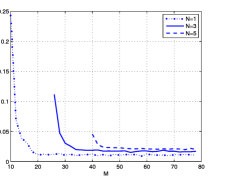
(a)

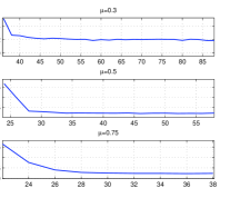
(b)

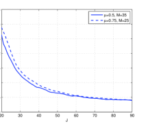
(c)

Figure 6: (a) Decay of the reconstruction error with increased number of samples for multipulse signals with $N=1,3,5$ pulses, pulse width $W=0.18$ms and frame redundancy $\mu=0.5$. (b) Comparison of performance for signals with $N=3$, $W=0.24$ms using different frames with $\mu=0.3$, $\mu=0.5$ and $\mu=0.75$. (c) Comparison of the relative error with respect to the number of channels $J$ for multipulse essentially bandlimited signals with $N=3$, $W=0.18$ms, $S=2$ with respect to different frames.

We now present some numerical experiments illustrating the recovery of multipulse signals.

We tested our sampling scheme using Monte Carlo simulations averaged over $500$ trials on a range of multipulse signals of duration $\beta=22$ms. The pulses making up the signals were chosen at random from a set of five different pulses: cosine, Gaussian, B-spline of order $3$ and $5$, and rectangular pulse. The locations of the pulses were also chosen at random. We varied the number of pulses $N=1,3,5$, the maximal width $W=0.18,0.24$ms of the pulse, and the redundancy $\mu=0.3,0.5,0.75$ of the frame. Throughout the experiments we chose $\mathbf{D}=\mathbf{I}$ and $\mathbf{C}$ as a Bernoulli random matrix. We measured the relative error $\lVert f-\widetilde{f}\rVert/\lVert f\rVert_{2}$. For redundancy $\mu=0.3$ we chose a Gabor frame with window being B-spline of order three, for $\mu=0.5$ the window was a cosine, and for $\mu=0.75$ we chose the truncated Gaussian.

Fig. 6(a) depicts the decrease in the reconstruction error with increased number of samples $M$ for different values of $N$ and $W=0.18$ms. We used a tight Gabor frame with a cosine window and redundancy $\mu=0.5$. The $M$ is dictated by the the number of pulses and frame redundancy, and it has to be at least $2\lceil 2\mu^{-1}\rceil N$. Meaning, that for multipulse signals with $N=1$ pulses, $M\geq 8$, for $N=3$ we have $M\geq 24$, and for $N=5$ it has to be $M\geq 40$. As expected, the sparser the signal, the less samples are needed for a good reconstruction. The number of samples in time can be significantly reduced if sparsity is taken into account. Without any knowledge on the sparsity we would have to take $K=241$ time samples for signals with $N=5$ pulses, and with $L_{0}=5$ that would result in the reconstruction error of $0.05$. However, when sparsity is taken into account, already $M=40$ samples suffice to achieve the same reconstruction error. Therefore reducing the number of samples by a factor of six. When $N=3$, to achieve reconstruction error of $0.05$ we need $M=28$ samples in time, and $M=12$ for signals with $N=1$.

In Fig. 6(b) we considered the influence of the Gabor frame on the reconstruction error and the number of samples $M$ involved. We tested the system for signals with $N=3$ pulses of width no more than $W=0.24$ms and $L_{0}=5$. The least number of samples $K=121$ is achieved with $\mu=0.75$ and at the same time with $M=25$ we achieve a good reconstruction. The value of $M$ necessary for a good reconstruction increases with the increase of redundancy. Without knowing the sparsity structure of the signal in time, we would have to take $K=271$ samples for $\mu=0.3$, and $K=120$ for $\mu=0.5$. When sparsity is exploited, we can reduce that number to $M=45$ and $M=27$, respectively.

We then examined the performance of our sampling scheme on signals comprising three pulses of width no more than $W=0.18$ms, that are additionally essentially multiband with two bands. Fig. 6(c) depicts the decay of reconstruction error with the increase of $J$ for two different frames: one is a tight frame with cosine window and redundancy $\mu=0.5$ and second, a frame with Gaussian window and redundancy $\mu=0.75$. The sampling system was tested with the matrix $\mathbf{D}$ being the random Fourier matrix and $\mathbf{C}$ a Bernoulli random matrix. For example, when a frame is of redundancy $\mu=0.5$ and no sparsity is taken into account then we need $K=241$ and $L=91$ samples to achieve a reconstruction error of $0.07$. On the other hand, with sparsity being exploited we can use only $M=35$ and $J=40$ for a similar reconstruction quality, resulting in a twelvefold reduction in the number of samples.

X Conclusions

We presented an efficient sampling scheme for multipulse signals, which is designed independently of the time support of the input signal. Our system allows to sample multipulse signals at the minimal rate, far below Nyquist, without any knowledge of the pulse shapes or its locations. The scheme fits into the broad context of Xampling - a recent sub-Nyquist sampling paradigm for analog signals. Our architecture relies on Gabor frames which lead to sparse expansions of multipulse signals, and consists of modulating the signal with several waveforms followed by integration. We showed that the Gabor coefficients, necessary for reconstruction, can be recovered from the samples of the system by utilizing CS techniques. The number of necessary samples depends on the desired accuracy of the approximation, essential bandwidth of the signal, and redundancy factor $\mu$ related to the Gabor frame, and equals $4\Omega^{\prime}NW\mu^{-1}$. The sampling rate can be further reduced if the signal is additionally sparse in frequency. We also showed that the proposed sampling and recovery technique is stable with respect to noise and mismodeling.

Appendix A Proof of Theorem III.1

The proof is rooted in that of Theorem 3.6.15 in [24] with appropriate adjustments. Since $\mathcal{G}(g,a,b)$ is a Gabor frame, $f(t)$ admits a decomposition

$$f=\sum_{k=-K_{0}}^{K_{0}}\sum_{l\in\mathbb{Z}}z_{k,l}M_{bl}\,T_{ak}\,\gamma\,.$$

Let $\epsilon_{B}>0$. The bandlimited ${S_{0}}$ functions are dense in ${S_{0}}$, therefore, there exists $g_{c}\in{S_{0}}$ bandlimited to some $[-B/2,B/2]$, such that

$$\lVert g-g_{c}\rVert_{{S_{0}}}\leq\epsilon_{B}\lVert g\rVert_{{S_{0}}}\,.$$

Since $f(t)$ is an essentially bandlimited function, there exists a function $f_{c}(t)$ bandlimited to $[-\Omega/2,\Omega/2]$, such that

$$\lVert f-f_{c}\rVert_{2}\leq\epsilon_{\Omega}\lVert f\rVert_{2}\,.$$

Consequently, $\lvert z_{k,l}\rvert=\lvert\langle\widehat{f_{c}},M_{-ak}\,T_{bl}\widehat{g_{c}}\rangle\rvert\neq 0$ only for those $\ell$ such that $\mbox{supp}\,\widehat{f_{c}}\cap(\mbox{supp}\,\widehat{g_{c}}+bl)\neq\emptyset$, that is

$$[-\Omega/2,\Omega/2]\cap[bl-B/2,bl+B/2]\neq\emptyset\,.$$

The fact that $f_{c}(t)$ and $g_{c}(t)$ are bandlimited implies that there are only a finite number of values $\ell$ for which $V_{g_{c}}f_{c}(ak,bl)\neq 0$. Let $L_{0}$ be the smallest integer such that $\lvert V_{g_{c}}f_{c}(ak,bl)\rvert=0$ for $\lvert l\rvert>L_{0}$. The exact value of $L_{0}$ can be calculated as

$$L_{0}=\left\lceil\frac{\Omega+B}{2b}\right\rceil-1\,.$$

Define a sequence $d_{k,l}$ as

$$d_{k,l}=\left\{\begin{array}[]{ll}z_{k,l}\,,&\lvert k\rvert\leq K_{0},\,\,\lvert l\rvert>L_{0}\\ 0\,,&\mbox{else.}\end{array}\right.$$

Then $\lvert d_{k,l}\rvert\leq\lvert V_{g-g_{c}}f(ak,bl)+V_{g_{c}}(f-f_{c})(ak,bl)\rvert$ for all $k,l\in\mathbb{Z}$, and

$$\Big{\lVert}f -\sum_{k=-K_{0}}^{K_{0}}\sum_{l=-L_{0}}^{L_{0}}z_{k,l}M_{bl}\,T_{ak}\,\gamma\Big{\rVert}_{2}=$$

$$=\Big{\lVert}\sum_{k\in\mathbb{Z}}\sum_{l\in\mathbb{Z}}d_{k,l}M_{bl}\,T_{ak}\,\gamma\Big{\rVert}_{2}\leq C_{a,b}\lVert\gamma\rVert_{{S_{0}}}\lVert d\rVert_{{\ell_{2}}}$$

$$\leq C_{a,b}\lVert\gamma\rVert_{{S_{0}}}\big{(}\lVert V_{g-g_{c}}f\rVert_{{\ell_{2}}}+\lVert V_{g_{c}}(f-f_{c})\rVert_{{\ell_{2}}}\big{)}$$

$$\leq C_{a,b}^{2}\lVert\gamma\rVert_{{S_{0}}}\lVert g\rVert_{{S_{0}}}(\epsilon_{B}+\epsilon_{\Omega})\lVert f\rVert_{2}\,$$

where we first used the boundedness of the analysis operator related to $g(t)$ and then the synthesis operator related to $\gamma(t)$ whenever $g$ and $\gamma$ are in ${S_{0}}$.

Appendix B $S-$term approximation of $\mathbf{Z}$

We show here the existence of an $S-$term approximation of $\mathbf{Z}$.

Lemma B.1.

Let $f\in\mathcal{MP}_{ess}(N,W,\beta,\Omega)$ be $\delta_{W}-$essentially multipulse and $\mathcal{G}(g,a,b)$ be a Gabor frame with $g$ compactly supported on $[-W/2,W/2]$ and $a=\mu W$, $b=1/W$ for some $0<\mu<1$. Then there exists a subset $\mathcal{S}$ of $\{-K_{0},\ldots,K_{0}\}$ such that

$$\lVert\mathbf{Z}-\mathbf{Z}^{\mathcal{S}}\rVert_{2,1}\leq\delta_{W}\sqrt{K}C_{a,b}\lVert g\rVert_{{S_{0}}}\lVert f\rVert_{2}\,,$$

where $\mathbf{Z}^{\mathcal{S}}$ consists of rows of $\mathbf{Z}$ indexed by $\mathcal{S}$, $K=2K_{0}+1$ and $\lVert\mathbf{Z}\rVert_{2,1}=\sum_{k=-K_{0}}^{K_{0}}(\sum_{l=-L_{0}}^{L_{0}}\lvert z_{k,l}\rvert^{2})^{1/2}$.

Proof.

Let $f_{p}\in\mathcal{MP}(N,W,\beta,\Omega)$ be a multipulse $\delta_{W}-$approximation of $f$. Then $V_{g}f_{p}(ak,bl)=0$ for all $\lvert k\rvert>K_{0}$, and the column vectors $[V_{g}f_{p}(-aK_{0},bl),\ldots,V_{g}f_{p}(aK_{0},bl)]^{T}$, $\lvert l\rvert\leq L_{0}$, are all jointly sparse with $\lceil 2\mu^{-1}\rceil N$ nonzero coefficients. Let $\mathcal{S}$ denote the index set of nonzero coefficients. For $\lvert\ell\rvert\leq L_{0}$, let $\mathbf{Z}^{\mathcal{S}}[l]$ be vectors with coefficients $z^{\mathcal{S}}_{k,l}$ defined by

$$z^{\mathcal{S}}_{k,l}=\left\{\begin{array}[]{ll}z_{k,l}&k\in\mathcal{S}\\ 0&k\notin\mathcal{S}\,.\end{array}\right.$$

Then $\mathbf{Z}^{\mathcal{S}}[l]$ is the best $\lceil 2\mu^{-1}\rceil N-$term approximation of $\mathbf{Z}[l]$, for each $\ell$. Note that $\lvert z_{k,l}-z^{\mathcal{S}}_{k,l}\rvert\leq\lvert V_{g}(f-f_{p})(ak,bl)\rvert$ for all $k$ and $\ell$, so that

$$\lVert\mathbf{Z} -\mathbf{Z}^{\mathcal{S}}\rVert_{2,1}=\sum_{k=-K_{0}}^{K_{0}}\left(\sum_{l=-L_{0}}^{L_{0}}\lvert z_{k,l}-z^{\mathcal{S}}_{k,l}\rvert^{2}\right)^{1/2}$$

$$\leq\sum_{k=-K_{0}}^{K_{0}}\left(\sum_{l=-L_{0}}^{L_{0}}\lvert V_{g}(f-f_{p})(ak,bl)\rvert^{2}\right)^{1/2}$$

$$\leq\sum_{k=-K_{0}}^{K_{0}}\lVert V_{g}(f-f_{p})(ak,\cdot)\rVert_{{\ell_{2}}}\leq\sqrt{K}\lVert V_{g}(f-f_{p})\rVert_{{\ell_{2}}}$$

$$\leq\sqrt{K}C_{a,b}\lVert g\rVert_{{S_{0}}}\lVert f-f_{p}\rVert_{2}\leq\delta_{W}\sqrt{K}C_{a,b}\lVert g\rVert_{{S_{0}}}\lVert f\rVert_{2}\,,$$

completing the proof. ∎

References

- [1] G. B. Folland and A. Sitaram, “The uncertainty principle: a mathematical survey,” J. Fourier Anal. Appl.
- [2] P. L. Butzer and W. Splettstösser, “A sampling theorem for duration-limited functions with error estimates,” Information and Control, vol. 34, 1977.
- [3] P. L. Butzer and R. L. Stens, “Sampling theory for not necessarily band-limited functions: A historical overview,” SIAM Review, vol. 34, no. 1, 1992.
- [4] K. Gröchenig, Foundations of Time-Frequency Analysis. Birkhäuser, Boston, 2001.
- [5] J. J. Benedetto, C. Heil, and D. F. Walnut, “Gabor systems and the Balian-Low theorem,” in Gabor Analysis and Algorithms: Theory and Applications, H. Feichtinger and T. Strohmer, Eds. Birkhäser, Boston, MA, 1998.
- [6] M. Vettereli, P. Marziliano, and T. Blu, “Sampling signals with finite rate of innovation,” IEEE Trans. Signal Processing, vol. 50, no. 6, pp. 1417–1428, June 2002.
- [7] P. L. Dragotti, M. Vettereli, and T. Blu, “Sampling moments and reconstructing signals of finite rate of innovation: Shannon meets Strang-Fix,” IEEE Trans. Signal Processing, vol. 55, no. 5, pp. 1741–1757, May 2007.
- [8] K. Gedalyahu, R. Tur, and Y. C. Eldar, “Multichannel sampling of pulse streams at the rate of innovation,” IEEE Trans. on Signal Processing, vol. 59, no. 4, pp. 1491–1504, Apr. 2011.
- [9] R. Tur, Y. C. Eldar, and Z. Friedman, “Innovation rate sampling of pulse streams with application to ultrasound imaging,” IEEE Trans. on Signal Processing, vol. 59, no. 4, pp. 1827–1842, Apr. 2011.
- [10] J. Berent, P. L. Dragotti, and T. Blu, “Sampling piecewise sinusoidal signals with finite rate of innovation methods,” IEEE Trans. Signal Processing, vol. 58, no. 2, pp. 613–625, Feb. 2010.
- [11] W. U. Bajwa, K. Gedalyahu, and Y. C. Eldar, “Identification of parametric underspread linear systems and super-resolution radar,” IEEE Trans. Signal Processing, vol. 59, no. 6, pp. 2548–2561, June 2011.
- [12] J. A. Tropp, A. C. Gilbert, and M. J. Strauss, “Algorithms for simultaneous sparse approximation. Part I: Greedy pursuit,” Signal Processing, vol. 86, 2006.
- [13] S. F. Cotter, B. D. Rao, K. Engan, and K. Kreutz-Delgado, “Sparse solutions to linear inverse problems with multiple measurement vectors,” IEEE Trans. Signal Processing, vol. 53, no. 7, pp. 2477–2488, June 2005.
- [14] M. Mishali and Y. C. Eldar, “Reduce and boost: recovering arbitrary sets of jointly sparse vectors,” IEEE Trans. Signal Processing, vol. 56, no. 10, pp. 4692–4702, Oct. 2008.
- [15] M. Mishali, Y. C. Eldar, and A. Elron, “Xampling: Signal acquisition and processing in union of subspaces,” IEEE Trans. Signal Processing, vol. 59, no. 10, pp. 4719–4734, Oct. 2011.
- [16] M. Mishali, Y. C. Eldar, O. Dounaevsky, and E. Shoshan, “Xampling: Analog to digital at sub-Nyquist rates,” IET Journal of Circuits, Devices and Systems., vol. 5, no. 1, Jan. 2011.
- [17] M. Mishali and Y. C. Eldar, “From theory to practice: Sub-Nyquist sampling of sparse wideband analog signals,” IEEE Journal of Selected Topics on Signal Processing, vol. 4, no. 2, pp. 375–391, Apr. 2010.
- [18] ——, “Blind multi-band signal reconstruction: Compressed sensing for analog signals,” IEEE Trans. Signal Processing, vol. 57, no. 3, pp. 993–1009, Mar. 2009.
- [19] E. J. Candés, Y. C. Eldar, and D. Needell, “Compressed sensing with coherent and redundant dictionaries,” Numerical Analysis, vol. 31, no. 1, pp. 59–73, July 2011.
- [20] C. Hegde and R. G. Baraniuk, “Sampling and Recovery of Pulse Streams,” IEEE Trans. Signal Processing, vol. 59, no. 4, pp. 1505–1517, Apr. 2011.
- [21] E. J. Candés, “The restricted isometry property and its implications for compressed sensing,” C. R. Acad. Sci. Paris, Ser. I, vol. 346, 2008.
- [22] I. Daubechies, A. Grossmann, and Y. Meyer, “Painless nonorthogonal expansions,” J. Math. Phys., vol. 27, no. 5, 1986.
- [23] O. Christensen, “Pairs of dual Gabor frame generators with compact support and desired frequency localization,” Applied and Computational Harmonic Analysis, vol. 20, no. 3, 2006.
- [24] H. Feichtinger and G. Zimmermann, “A Banach space of test functions for Gabor analysis,” in Gabor Analysis and Algorithms: Theory and Applications, H. Feichtinger and T. Strohmer, Eds. Birkhäser, Boston, MA, 1998.
- [25] I. Daubechies, Ten Lectures on Wavelets. SIAM, Society for Industrial and Applied Mathematics, 1992.
- [26] J. Chen and X. Huo, “Theoretical results on sparse representations of multiple-measurement vectors,” IEEE Trans. Signal Processing, vol. 54, no. 12, pp. 4634–4643, Nov. 2006.
- [27] M. E. Davies and Y. C. Eldar, “Rank awareness in joint sparse recovery,” to appear in IEEE Trans. on Info. Theory, Apr. 2010.
- [28] Y. C. Eldar and M. Mishali, “Robust recovery of signals from a structured union of subspaces,” IEEE Trans. Inform. Theory, vol. 55, no. 11, pp. 5302–5316, Nov. 2009.
- [29] R. G. Baraniuk, M. Davenport, R. DeVore, and M. Wakin, “A simple proof of restrcted isometry property for random matrices,” Const. Approx., 2007.
- [30] S. Mendelson, A. Pajor, and N. Tomczak-Jaegermann, “Uniform uncertainty principle for Bernoulli and subgaussian ensembles,” Constr. Approx., vol. 28, no. 3, 2008.
- [31] E. J. Candés and T. Tao, “Near optimal signal recovery from random projections: Universal encoding strategies?” IEEE Inf. Theory, vol. 52, no. 12, pp. 5406–5425, Nov. 2006.
- [32] M. Rudelson and R. Vershynin, “On sparse reconstruction from Fourier and Gaussian measurements,” Commun. Pure Appl. Math., vol. 61, no. 8, 2008.
- [33] Y. C. Eldar, “Compressed sensing of analog signals in shift-invariant spaces,” IEEE Trans. Signal Processing, vol. 57, no. 8, pp. 2986–2997, Aug. 2009.
- [34] K. Gedalyahu and Y. C. Eldar, “Time-delay estimation from low-rate samples: A union of subspaces approach,” IEEE Trans. on Signal Processing, vol. 58, no. 6, pp. 3017–3031, June 2010.
- [35] R. S. Laugesen, “Gabor dual spline windows,” Appl. Comput. Harmon. Anal., vol. 27, no. 2, 2009.
- [36] O. Christensen, H. O. Kim, and R. Y. Kim, “Gabor windows supported on and compactly supported dual windows,” Appl. Comp. Harm. Anal., vol. 28, 2010.
- [37] A. Ron and Z. Shen, “Frames and stable bases for shift-invariant subspaces of ,” Canad. J. Math, vol. 47, no. 5, 1995.
- [38] V. D. Prete, “Estimates, decay properties, and computation of the dual function for Gabor frames,” J. Fourier Anal. Appl., vol. 5, no. 6, 1999.