Anomalous diffusion in viscosity landscapes

Abstract

Anomalous diffusion is predicted for Brownian particles in inhomogeneous viscosity landscapes by means of scaling arguments, which are substantiated through numerical simulations. Analytical solutions of the related Fokker-Planck equation in limiting cases confirm our results. For an ensemble of particles starting at a spatial minimum (maximum) of the viscous damping we find subdiffusive (superdiffusive) motion. Superdiffusion occurs also for a monotonically varying viscosity profile. We suggest different substances for related experimental investigations.

1 Introduction

Brownian particle dynamics plays a key role for many transport processes in various disciplines. Even though a century has passed since the publication of Einstein’s seminal work on normal diffusion [1], the field of diffusion processes still attracts enormous interest [2, 3, 4, 5]. The essential signature of normal diffusion is the linear temporal growth of the mean square displacement of Brownian particles,

$$\langle x^{2}(t)\rangle\propto t^{\alpha}\,,$$ (1)

with $\alpha=1$, whereas for $\alpha\neq 1$ the notion anomalous diffusion has been introduced [6, 7, 8, 9, 10]. Being not only of fundamental but also of great technological relevance, the dynamical processes underlying anomalous diffusion phenomena have started to be investigated during recent decades in systems as diverse as collective ordering phenomena [11, 12], particle diffusion in mesoscopic systems [13, 14], or social networks [15]. At the same time, progress in single particle manipulation and detection on the $\mu$m and sub-$\mu$m scale fostered investigations on random particle motions [16, 17, 18, 19, 20].

Diffusion processes with an exponent $0<\alpha<1$ in (1) are called subdiffusive. Several examples of such dynamic behavior are known for systems with a short inhomogeneity length scale, such as in amorphous semiconductors [10], groundwater motion [21], diffusion in gels [16], and in several biological systems such as in the bacterial cytoplasm [17], during protein diffusion through cell membranes [18], or as a possible method to detect the microstructures in actin filament networks [19]. Besides subdiffusive motion, heterogeneous parameter landscapes are considered to be important also in generalized reaction-diffusion systems and for bifurcations in pattern forming systems in general [17, 22, 23, 24]. Conversely, superdiffusive processes are random motions with an exponent $\alpha>1$, which are found in rather different areas of natural and social sciences. Superdiffusion tends to occur in active and driven systems where random steps are interrupted by intermediate and nearly deterministic motion, such as for particles in (turbulent) random velocity fields [25, 26], during cell migration [20], for active transport in cells [13], or during the spread of diseases [15].

Another class of Brownian motion that attracted remarkable interest recently is described by a nonlinear Langevin equation with a velocity dependent viscous damping coefficient which is used as a model for active and relativistic motion [27, 28, 29, 30] as well as in the context of ratchet models [31].

Here, we investigate the effects of inhomogeneous viscosities on the one-dimensional dynamics of Brownian particles, considering viscosity variations, which are slow on the scale of the particles’ random steps. In this case, the interplay of a diffusing particle with its inhomogeneous surrounding leads to intermediate regimes of anomalous diffusion, similar to the intermediate Rouse regime of diffusion of polymer segments [32]. Near a viscosity minimum we find subdiffusion, whereas superdiffusive behavior is found near a viscosity maximum and for monotonously varying viscosity profiles. In all three cases the particles’ probability distribution is found to be non-Gaussian.

Our analysis is based on a nonlinear Langevin equation and the appendant Fokker-Planck equation, which are presented in section 2 together with the spatially varying model viscosities considered in this work. In section 3 we calculate scaling formulas for the mean square displacement and analytical solutions of the Fokker-Planck equation for several limiting cases. These results are compared with numerical simulations in section 4. Finally, we comment on possible experimental realizations within our summary in section 5.

2 Model

2.1 Langevin and Fokker-Planck equation

The one-dimensional Langevin equation for the velocity $v(t)$ of a particle of mass $m$ and radius $a$ immersed in a medium with a spatially varying viscosity landscape $\eta(x)$ is given by

$$\dot{v}(t)=-\gamma(x)v+g(x)\xi(t)\,,$$ (2)

with $\gamma(x)=6\pi a\eta(x)/m$ as the associated damping. The right hand side includes white noise $\xi(t)$ characterized by

$$\langle\xi(t)\rangle=0\,\qquad\mbox{and}\qquad\langle\xi(t)\xi(t^{\prime})\rangle=\delta(t-t^{\prime})\,.$$ (3)

For the noise strength $g(x)$ we assume a local fluctuation-dissipation relation [33]

$$g^{2}(x)=\frac{2\gamma(x)k_{B}T}{m}\,$$ (4)

with $k_{B}$ being the Boltzmann constant and $T$ denoting the constant temperature. In the overdamped limit, i. e. for times longer than the characteristic time $\gamma^{-1}$, a Langevin equation for the particle’s position can be derived from (2) by using the method of adiabatic elimination [3, 5, 34]. In Ito’s interpretation it takes the form

$$\dot{x}(t) =\frac{k_{B}T}{m}\frac{\partial}{\partial x}\frac{1}{\gamma(x)}+\sqrt{\frac{2k_{B}T}{m\gamma(x)}}\ \xi(t)\,.$$ (5)

The corresponding Fokker-Planck equation for the probability density of a particle $P(x,t)$ can be deduced straightforwardly from (5),

$$\frac{\partial P(x,t)}{\partial t} =\frac{\partial}{\partial x}\left[D(x)\frac{\partial P(x,t)}{\partial x}\right]\,,$$ (6)

with a spatially varying diffusion coefficient $D(x)=k_{B}T/(m\gamma(x))$. The Brownian dynamics of an ensemble of test particles is investigated on the basis of (2), (5) and (6) with their initial positions at $x(t=0)=0$.

2.2 Model viscosities

Spatially varying viscosities may be realized with organic gradient materials, where for instance the composition or the degree of polymerization changes in space [35, 36]. In photorheological fluids, as another example, the viscosity can be tuned by a spatially varying illumination intensity [37]. A further class with the possibility of inhomogeneous viscosities are binary-fluid mixtures. Here spatial variations of the concentration of the two constituents may be driven by temperature modulations via the Soret effect [38]. If both constituents have sufficiently different viscosities the thermally induced concentration variations are accompanied by spatial viscosity changes. For materials with a strong Soret effect, quantified by the Soret coefficient $S_{T}$, small temperature gradients are sufficient to generate large concentration and therefore large viscosity gradients, so that the direct effects of temperature gradients can be neglected. Suchlike experimentally favorable large values of $S_{T}$ can be achieved by shifting the mean temperature of the binary fluid in the one-phase region close to the critical temperature of the mixture, where a transition to the two-phase region takes place [41, 42, 43, 44].

For the materials mentioned above, one can imagine a number of spatially varying viscosities. A simple example of a viscosity of experimental relevance, being asymmetric with respect to the particles’ initial position at $x=0$, is

$$\eta(x)=\eta_{0}+\Delta\eta\tanh(x/L)\qquad\mbox{with}\qquad\eta_{0}>|\Delta\eta|>0\,,$$ (7)

which may be approximated for $|x|\ll L$ by

$$\eta(x)=\eta_{0}+\tilde{\eta}_{1}x\qquad\mbox{with}\qquad\tilde{\eta}_{1}=\Delta\eta/L\,.$$ (8)

Other generic viscosities are symmetric with a minimum or maximum at the particles’ starting point. As a representative model of these viscosities, showing a smooth change from the value $\eta_{0}$ at the extremum to the bulk value $\eta_{\infty}$, we choose

$$\eta(x) = \eta_{\infty}+\displaystyle\frac{\Delta\eta}{1+\left|x/L\right|^{\kappa}}\,,$$ (9)

with $\kappa>0$, the viscosity contrast $\Delta\eta=\eta_{0}-\eta_{\infty}$, and the characteristic length $L$. $\Delta\eta<0$ corresponds to a viscosity with a global minimum and $\Delta\eta>0$ to a maximum at $x=0$.

Equation (9) covers several limiting cases, which can be identified by expressing $\eta(x)$ in (9) for $|x|<L$ by a power series $\eta=\eta_{\infty}+\Delta\eta\sum_{n=0}^{\infty}(-1)^{n}\left|\frac{x}{L}\right|^{n\kappa}$ around $x=0$ and for $|x|>L$ by an asymptotic series $\eta=\eta_{\infty}+\Delta\eta\sum_{n=0}^{\infty}(-1)^{n}\left|\frac{x}{L}\right|^{-(n+1)\kappa}$. In distinct parameter ranges each series can reasonably be approximated by the leading contribution, which is feasible for the analytical considerations in section 3.

For a pronounced minimum, i. e. $\eta_{0}\ll\eta_{\infty}$, two approximations for $\eta(x)$ are useful: $\eta\simeq\eta_{0}~{}+\eta_{\infty}|x/L|^{\kappa}$ for $|x|\ll L$ respectively $\eta\simeq\eta_{\infty}\left(1-|x/L|^{-\kappa}\right)$ for $|x|\gg L$. The viscosity reaches its constant bulk value $\eta_{\infty}$ for large values of $|x|$ and for $\eta_{0}/\eta_{\infty}\ll|x/L|^{\kappa}\ll 1$ the latter approximation evaluates to the power law

$$\eta(x)\propto|x|^{\kappa}\,$$ (10)

that covers the $x$ dependence of $\eta(x)$ rather well. The validity of this power-law can be extended over a wider range with decreasing ratio $\eta_{0}/\eta_{\infty}$. For a pronounced maximum, i. e. $\eta_{0}\gg\eta_{\infty}$, we approximate $\eta(x)$ for $|x|\ll L$ as $\eta\simeq\eta_{0}\left(1-|x/L|^{\kappa}\right)$ and for $|x|\gg L$ as $\eta\simeq\eta_{\infty}+\eta_{0}|x/L|^{-\kappa}$. Accordingly for $1\ll|x/L|^{\kappa}\ll\eta_{0}/\eta_{\infty}$ the viscosity can again be simplified to a power law

$$\eta(x)\propto|x|^{-\kappa}\,,$$ (11)

while for $|x/L|^{\kappa}\gg\eta_{0}/\eta_{\infty}$ a nearly constant viscosity with $\eta(x)\approx\eta_{\infty}$ results. The range, where the viscosity can reasonably be approximated by a power-law, increases with rising values of the ratio $\eta_{0}/\eta_{\infty}$.

3 Scaling arguments and analytical solutions

For symmetric viscosity profiles, $\eta(|x|)$, we present a scaling analysis for the power law of the mean square displacement $\langle x^{2}\rangle\propto t^{\alpha}$ and in limiting cases exact solutions of the Fokker-Planck equation (6). For asymmetric profiles we use a perturbation series to gain the time evolution of the first moments.

3.1 Scaling arguments for symmetric viscosity profiles

The mean square displacement of a particle $\langle x^{2}(t)\rangle$ is commonly used to characterize its random motion. For a constant viscosity, the analytical solution of equation (2) takes the well-known form [2]: $\langle x^{2}(t)\rangle=\frac{2k_{B}T}{m\gamma^{2}}\left(e^{-\gamma t}+\gamma t-1\right)$. Beyond a short period of ballistic motion in the regime of normal diffusion, $t\gg\gamma^{-1}$, the mean square displacement increases linearly in time:

$$\langle x^{2}(t)\rangle=\frac{2k_{B}T}{m\gamma}t=\frac{k_{B}T}{3\pi a}\frac{t}{\eta}=Q\frac{t}{\eta}\,.$$ (12)

In order to achieve progress by analytical calculations also for spatially varying and symmetric viscosity profiles $\eta(x)=\eta(|x|)$, we use (12) with the replacement $\eta\to\eta(|x|)$ and simultaneously the substitution $|x|\to\sqrt{\langle x^{2}(t)\rangle}$. The resulting expression,

$$\langle x^{2}(t)\rangle=Q~{}\frac{t}{\eta\!\left(\sqrt{\langle x^{2}(t)\rangle}\right)}\,,$$ (13)

is further analyzed for different regimes of the model viscosity (9).

Within a very short time interval, where $\langle x^{2}\rangle\approx 0$ holds, the model viscosity $\eta\!\left(\sqrt{\langle x^{2}(t)\rangle}\right)$ given by (9) can be approximated by $\eta_{0}$ (regime I) and in the long time regime, i. e. for $\langle x^{2}\rangle\to\infty$, by $\eta_{\infty}$ (regime III). In both cases one obtains with equation (13) normal diffusion:

$$\langle x^{2}(t)\rangle=\frac{Q}{\eta_{0}}~{}t\qquad\mathrm{and}\qquad\langle x^{2}(t)\rangle=\frac{Q}{\eta_{\infty}}~{}t\,.$$ (14)

Between these two regimes, one finds regime II with a power-law behavior $\eta(x)=\tilde{\eta}~{}|x|^{\beta}$ respectively $D(x)=\tilde{D}|x|^{-\beta}$ (see also (6), (10) and (11)) for $\beta=\kappa>0$ near a viscosity minimum and $\beta=-\kappa<0$ near a maximum. This yields together with (13)

$$\langle x^{2}(t)\rangle=Q~{}\frac{t}{\tilde{\eta}~{}\langle x^{2}(t)\rangle^{\beta/2}}\,,$$ (15)

which is the basis of the prediction of anomalous diffusion in regime II:

$$\langle x^{2}(t)\rangle=\left(\frac{Q}{\tilde{\eta}}\right)^{\alpha}~{}t^{\alpha}\qquad\mathrm{with}\qquad\alpha=\frac{2}{2+\beta}\,.$$ (16)

Near a viscosity minimum, $\beta>0$, one has subdiffusion with $\alpha<1$ and near a viscosity maximum, $\beta<0$, superdiffusion with $\alpha>1$. For $\beta=-2$ the scaling formula (16) breaks down and the overdamped Langevin equation (5) evaluates to $\dot{x}=x~{}[2\tilde{D}+(2\tilde{D})^{1/2}\,\xi(t)]\,$, which describes the so-called geometric Brownian motion. In this case the power law in equation (1) is replaced by an exponential time dependence of the second moment $\langle x^{2}(t)\rangle\propto e^{6\tilde{D}t}$ [45].

During the crossovers between the three regimes the exponent $\alpha$ of the mean square displacement, $\langle x^{2}(t)\rangle\propto t^{\alpha}$, varies as a function of time from 1 in regime I to $2/(2+\beta)$ in regime II and back to 1 in regime III. The location of regime II follows by translating the respective spatial ranges described in section 2.2 onto time via (13):

$$\frac{2L^{2}\eta_{0}}{Q}\left(\frac{\eta_{0}}{\eta_{\infty}}\right)^{2/\kappa}\ll t\ll\frac{L^{2}\eta_{\infty}}{2Q}\qquad\mathrm{(subdiffusion)}\,,$$ (17)

$$\frac{L^{2}\eta_{0}}{2Q}\ll t\ll\frac{2L^{2}\eta_{\infty}}{Q}\left(\frac{\eta_{0}}{\eta_{\infty}}\right)^{2/\kappa}\qquad\mathrm{(superdiffusion)}\,.$$ (18)

Therefore, the experimental accessibility of the anomalous regime II is enhanced, when the viscosity contrast $|\Delta\eta|=|\eta_{0}-\eta_{\infty}|$ is enlarged.

3.2 Fokker-Planck equation: Solutions for symmetric and asymmetric viscosity profiles

For a power law approximation $\eta(x)\propto|x|^{\beta}$ of symmetric viscosity profiles in regime II the diffusion coefficient is given by $D(x)=\tilde{D}|x|^{-\beta}$. In this case, the Fokker-Planck equation (6) with the initial condition $P(x,0)=\delta(x)$ can be solved analytically for $\beta>-2$ by using the ansatz

$$P(x,t)=\frac{k}{t^{1/(2+\beta)}}\exp\!\left(-\frac{|x|^{2+\beta}}{t\tilde{D}(2+\beta)^{2}}\right)\,,$$ (19)

with $k=\frac{2+\beta}{2}\,[\tilde{D}(2+\beta)^{2}]^{-1/(2+\beta)}\,\Gamma^{-1}(\frac{1}{2+\beta})$ being a normalization constant. With this expression the second moment can be evaluated exactly to

$$\langle x^{2}\rangle\,=\frac{\Gamma(\frac{3}{2+\beta})}{\Gamma(\frac{1}{2+\beta})}\,\left[\tilde{D}(2+\beta)^{2}\,t\right]^{2/(2+\beta)}\,\propto\,t^{2/(2+\beta)}\,,$$ (20)

which follows the identical power-law in time as in (16) and supports the validity of the assumptions made for the scaling argument in section 3.1. The odd moments vanish because of the $\pm x$ symmetry and the even moments deviate for $\beta\neq 0$ from the case of normal diffusion. As an example we consider the kurtosis $K$, which is a quantity for the distribution’s peakedness and defined as 4th central moment divided by the 2nd central moment [8]. For (19) it takes the form $K=\Gamma\!\left(\frac{1}{2+\beta}\right)\Gamma\!\left(\frac{5}{2+\beta}\right)\Gamma^{-2}\!\left(\frac{3}{2+\beta}\right)$, indicating a normal distribution ($K=3$, i. e. mesokurtic) for $\beta=0$, a distribution with a high sharp peak ($K>3$, i. e. leptokurtic) for $-2<\beta<0$, and a flat-topped distribution ($K<3$, i. e. platykurtic) for $\beta>0$.

To gain insight in the diffusion for a asymmetric linear viscosity profile as in equation (8), respectively for the corresponding diffusion coefficient, $D(x)=\tilde{D}(\eta_{0}+\tilde{\eta}_{1}x)^{-1}$ with $\tilde{D}=\frac{k_{B}T}{6\pi a}$, we derive the equation for the $n$-th moment,

$$\frac{\partial}{\partial t}\langle x^{n}\rangle=n\left\langle\frac{\partial}{\partial x}D(x)x^{n-1}\right\rangle\,,$$ (21)

as a function of $D(x)$ by a double integration by parts of the Fokker-Planck equation (6). In order to proceed we expand on the right hand side of equation (21) the term inside the brackets with respect to powers of $x$. The resulting system of coupled differential equations for the moments $\langle x^{n}\rangle$ is solved in the limit $\tilde{\eta}_{1}x/\eta_{0}\ll 1$ by a power series ansatz in $\tilde{\eta}_{1}$. This leads together with the initial conditions $\langle x^{n}\rangle(0)=0$ to the following approximations for the first three moments:

$$\langle x\rangle = -\frac{\tilde{\eta}_{1}\tilde{D}}{\eta_{0}^{2}}~{}t-\frac{4\tilde{\eta}_{1}^{3}\tilde{D}^{2}}{\eta_{0}^{5}}~{}t^{2}+\mathcal{O}(\tilde{\eta}_{1}^{5})\,,$$ (22a)

$$\langle x^{2}\rangle = ~{}\frac{2\tilde{D}}{\eta_{0}}~{}t+\frac{8\tilde{\eta}_{1}^{2}\tilde{D}^{2}}{\eta_{0}^{4}}~{}t^{2}+\frac{280\tilde{\eta}_{1}^{4}\tilde{D}^{3}}{3\eta_{0}^{7}}~{}t^{3}+\mathcal{O}(\tilde{\eta}_{1}^{6})\,,$$ (22b)

$$\langle x^{3}\rangle = -\frac{12\tilde{\eta}_{1}\tilde{D}^{2}}{\eta_{0}^{3}}~{}t^{2}-\frac{140\tilde{\eta}_{1}^{3}\tilde{D}^{3}}{\eta_{0}^{6}}~{}t^{3}+{\mathcal{O}}(\tilde{\eta}_{1}^{5})\,.$$ (22c)

According to (22b) anomalous diffusion can be expected to occur for linearly varying viscosity profiles, too. Further, the onset of anomalous diffusion is governed by the ratio $\tilde{\eta}_{1}/\eta_{0}$: The larger this ratio the sooner the transition to anomalous diffusion takes place. Asymmetric viscosity profiles lead to a mean particle drift towards the region with lower viscosity as indicated by (22a). It is also a remarkable property of each of the three moments that the sign of the leading contributions does not alternate.

4 Numerical results

The results of the previous section are substantiated in the following by comparisons with numerical simulations of the Langevin equation (2) and the Fokker-Planck equation (6) for different spatially varying viscosities.

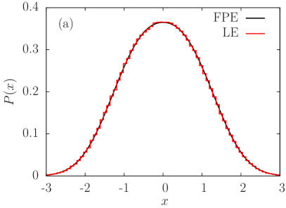
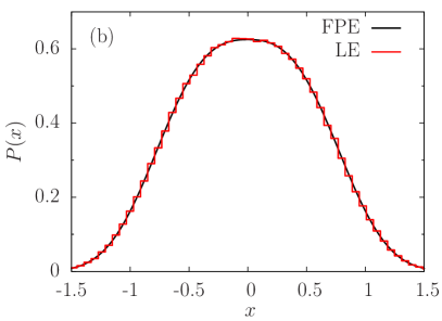
Figure 1: The probability density function $P(x)$ at $t=10$ is given for $\eta(x)=\eta_{0}+\tilde{\eta}|x|$ with $\eta_{0}=10$ and $\tilde{\eta}=10$ in (a) and $\tilde{\eta}=100$ in (b). The solid line (FPE) is obtained as a numerical solution of (6) with a narrow initial distribution and the step function (LE) by integrating (2) for $10^{6}$ independent trajectories with the starting point at $x=0$.

The Fokker-Planck equation (6) with a spatially varying damping is derived from (2) under the assumption $t\gg\gamma^{-1}$ [34]. For the symmetric viscosity $\eta(x)=\eta_{0}+\tilde{\eta}|x|$ with the minimal value $\eta_{0}=10$ and two different slopes $\tilde{\eta}=10$ and $\tilde{\eta}=100$, the distribution $P(x)$ is determined in figure 1 at the time $t=10\gg\gamma_{\mathrm{min}}^{-1}=0.1$ by solving either the Fokker-Planck equation (6) (black solid curve) or by integrating the Langevin equation (2) for an ensemble of $10^{6}$ particles (red step function). The inequality $t\gg\gamma^{-1}$ is not always fulfilled as good as in figure 1, but the solutions of (6) are also for shorter times and stronger variations of $\eta(x)$ often in good agreement with the solutions of (2).

There is a further aspect to be drawn from the profiles of the probability distribution $P(x)$ in the anomalous regime. After the short normal diffusion in regime I, $P(x)$ at $t=1$ deviates in regime II from a Gaussian profile as shown in figure 2. In part (a) the red curve of $P(x)$ is determined numerically by solving (6) for the spatially varying viscosity $\eta(x)=\eta_{0}+x^{2}$ with a small minimal viscosity $\eta_{0}=0.01$. It is compared with the analytical solution of the Fokker-Planck equation in (19) for $\eta=x^{2}$ (blue dashed line) and we find a nearly perfect agreement between both approaches in figure 2. Deviations grow by increasing the viscosity minimum $\eta_{0}$ in our simulations. Both curves in figure 2(a) deviate, however, significantly from a Gaussian distribution (green dotted line) with the same second moment. As predicted in section 3.2 the distribution is platykurtic for $\beta>0$, which can be explained as follows. Due to the small minimal viscosity $\eta_{0}$ at the starting point at $x=0$, particles quickly diffuse away. This reduces the probability to find a particle at $x=0$ and simultaneously enhances $P(x)$ in a wider neighborhood of the minimum of $\gamma(x)$, compared to the case of a constant damping with a Gaussian distribution. On the other hand, a viscosity increasing strongly as a function of $|x|$ impedes quick particle diffusion away from the minimum. This reduces the probability to find a particle at larger distances compared to a Gaussian distribution.

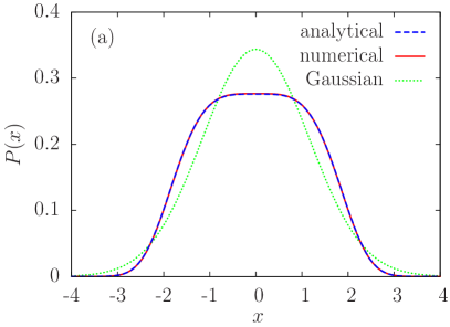
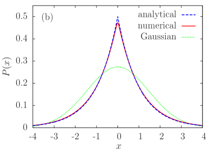
Figure 2: The probability distribution $P(x)$ at $t=1$ for two different viscosities: In (a) $\eta(x)=0.01+x^{2}$ with a minimum at $x=0$ and in (b) $\eta(x)=(0.001+|x|)^{-1}$ with a maximum at $x=0$. The red line in each part is obtained by numerical integration of (6) and the nearly identical blue dashed curve is the analytical solution given by (19) for $\eta(x)\propto x^{2}$ in (a) and $\eta(x)\propto|x|^{-1}$ in (b). In both parts $P(x)$ is compared with a Gaussian profile (green dotted line) having the same second moment.

With a viscosity maximum at the starting point of the particles the situation is similar, as illustrated by the distribution in figure 2(b). Here the numerical solution $P(x)$ of the Fokker-Planck equation (red curve) is obtained for the viscosity $\eta(x)=(0.001+|x|)^{-1}$ and is compared with the analytical solution given by (19) for $\eta(x)\propto|x|^{-1}$ (blue dashed curve). Only in the vicinity of the viscosity maximum at $x=0$ both approaches differ slightly. Again we find clear deviations from a Gaussian distribution with an identical second moment as described by the green dotted curve in figure 2(b). Since the Brownian dynamics is significantly reduced near the maximum of the damping at $x=0$, the particles move much slower away from the peak. This causes an enhancement of $P(x)$ around the maximum, compared to a Gaussian distribution. Thus the distribution is leptokurtic, in accordance with our predictions in section 3.2.

For a further analysis of the Brownian motion the mean square displacement $\langle x^{2}(t)\rangle$ of the particle positions is calculated by integrating the Langevin equation (2) numerically for an ensemble of particles starting at $x=0$. Figure 3 exemplarily shows $\langle x^{2}(t)\rangle$ as a function of time for two different spatially varying viscosities. In each case and independent from the particular viscosity landscape, the mean square displacement is characterized by the initial regime I of normal diffusion, marked by the dotted lines.

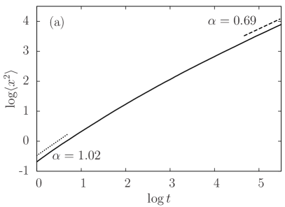
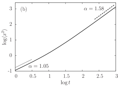
Figure 3: The mean square displacement $\langle x^{2}(t)\rangle$ as obtained by a numerical integration of (2) for two different model viscosities $\eta(x)$. In (a) $\eta(x)=10+|x|$ has a minimum at $x=0$, whereas in (b) one has for $|x|<1$ the plateau $\eta(x)=20$, which is continued for $|x|\geq 1$ by the decaying function $\eta(x)=20|x|^{-3/4}$. The dashed and dotted lines in both parts indicate linear fits to the numerical data, whereby the slope $\alpha$ is explicitly shown.

Beyond this regime I, anomalous diffusion occurs with exponents $\alpha\not=1$, as long as the viscosity, experienced by the particles, does not reach a non-vanishing constant plateau value, as for instance for large $|x|$ in (9). In the vicinity of a viscosity minimum, subdiffusive Brownian motion with exponents $\alpha<1$ is found, as exemplified in figure 3(a) for $\eta(x)=\eta_{0}+\tilde{\eta}|x|$ with $\eta_{0}=10$ and $\tilde{\eta}=1$. At long times the mean square displacement $\langle x^{2}\rangle$ scales in the range of the dashed line with $t^{\alpha}$ and $\alpha=0.69$, in good agreement with the scaling result $\alpha=2/3$ predicted by formula (16) with $\beta=1$. The viscosity used in figure 3(b) has in a small range $|x|<1$ a constant maximum, $\eta(x)=20$, and then decays in the range $|x|>1$ according to the power law $\eta(x)=20|x|^{-3/4}$. A fit to the numerical data in the limit of long times yields in the range of the dashed line in figure 3(b) the exponent $\alpha=1.58$, deviating only slightly from the scaling prediction $\alpha=1.6$ obtained from (16) for $\beta=-0.75$.

The deviations between the exponent obtained in simulations and the exponent obtained via scaling arguments decrease at sufficiently long times either by reducing the minimal viscosity $\eta_{0}$ as in figure 3(a) or by shortening the plateau in figure 3(b). The scaling regimes I (normal diffusion) and II (anomalous diffusion) are separated by a transition period, where the crossover from $\alpha\simeq 1$ to $\alpha\neq 1$ takes place. This transition period may extend over several decades in time as for instance in figure 3(a) with $\tilde{\eta}/\eta_{0}=0.1$. Together with an exponent $\beta=1$ this causes a transition period lasting over more than three decades. In contrast, steep, nonlinear viscosity gradients obtained for $\beta>1$ and $\beta<0$ delimit the intermediate regime [see figure 3(b)].

viscosity $\eta(x)$	$\beta$	$\alpha$ (scaling)	$\alpha$ (numerically)
$0.01+|x|^{4}$	4	1/3	0.333
$0.01+|x|^{2}$	2	1/2	0.501
$0.01+|x|$	1	2/3	0.666
$0.01+|x|^{1/2}$	1/2	4/5	0.799
$0.01+|x|^{1/4}$	1/4	8/9	0.886
$(0.01+|x|^{1/2})^{-1}$	-1/2	4/3	1.330
$(0.01+|x|^{2/3})^{-1}$	-2/3	3/2	1.494
$(0.01+|x|)^{-1}$	-1	2	1.976
$(0.01+|x|^{4/3})^{-1}$	-4/3	3	2.963

Table 1: Chart of anomalous exponents $\alpha$ for spatially varying viscosities $\eta(x)$ obtained by the scaling formula (16) and via numerical solutions of (2) by fitting the resulting mean square displacement in regime II by the power law $\propto t^{\alpha}$. We find a good agreement in both generic cases: For subdiffusion ($\alpha<1$) with a minimum of $\eta(x)$ and for superdiffusion ($\alpha>1$) with a maximum of $\eta(x)$.

For a further examination of the scaling prediction in the anomalous regime II, different spatially varying viscosities were investigated numerically and in terms of the analytical scaling argument given by (16). As can be seen in table 1, the numerically and analytically obtained exponents $\alpha$ are in excellent agreement for several viscosities. In general, in the neighborhood of a viscosity minimum one obtains subdiffusive behavior, whereas in the vicinity of a viscosity maximum superdiffusive behavior is observed. For the viscosities in table 1 with a small value $\eta_{0}$ at the minimum or a large value at the viscosity maximum one finds according to (17) and (18) an early onset of the intermediate anomalous regime II. We would like to emphasize, that the viscosities discussed up to now are approximations of (9), which we used to demonstrate the good agreement between our scaling results and numerical simulations in the anomalous regime II. For the viscosity (9) regime II is also limited in time from above as described in the previous section by the characteristic times given in (17) and (18).

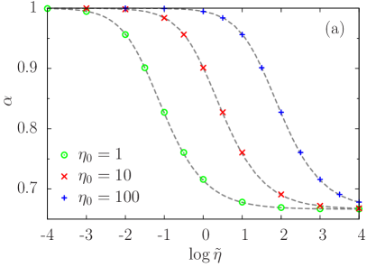
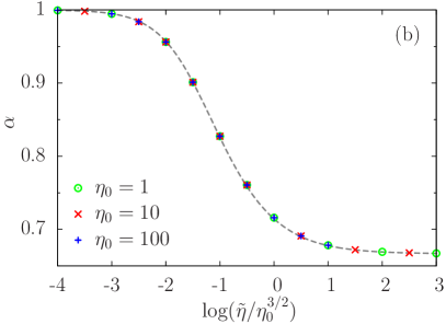
Figure 4: The scaling exponent $\alpha$ of the mean square displacement, $\langle x^{2}\rangle\propto t^{\alpha}$, is plotted in (a) for the symmetric viscosity $\eta(x)=\eta_{0}+\tilde{\eta}|x|$ as a function of the slope $\tilde{\eta}$ for three different values of $\eta_{0}=1,~{}10,~{}100$ and in part (b) as a function of the ratio $\tilde{\eta}/\eta_{0}^{3/2}$. $\alpha$ is obtained by fitting $\langle x^{2}\rangle\propto t^{\alpha}$ over a fixed time interval $0<t<10^{2}$ to numerical data created by integration of equation (6).

To investigate the crossover behavior between regime I and II, the Langevin and the Fokker-Planck equation were solved for the viscosity $\eta=\eta_{0}+\tilde{\eta}|x|$ up to the fixed time $T=100$ and for different values of $\eta_{0}$ and $\tilde{\eta}$. With this approach we mimic the limited time range available in experiments for detecting the anomalous regime. The numerical curves of the mean square displacement $\langle x^{2}(t)\rangle$ are fitted over the whole range $0\leq t\leq T$ by the power law $t^{\alpha}$ and the resulting exponent $\alpha$ is shown in figure 4 as function of the viscosity. The deviation of $\alpha$ from $\alpha=1$ grows, when the anomalous diffusion regime II occupies an increasing part of the interval $[0,T]$, i. e. when the inequality $\tilde{\eta}|x|>\eta_{0}$ holds for an increasing part of $[0,T]$. The two terms $\tilde{\eta}|x|$ and $\eta_{0}$ in the denominator of (13) become nearly equal at the time $t_{t}\sim\eta_{0}^{3}/\tilde{\eta}^{2}$. Hence, for decreasing values of $t_{t}$ the range of anomalous diffusion in $[0,T]$ increases as illustrated by the trend in figure 4(a). On the other hand, the anomalous fraction and therefore $\alpha$ can be kept constant by keeping $\tilde{\eta}^{2}/\eta_{0}^{3}$ constant, which is shown by figure 4(b).

The behavior of $\alpha$ in figure 4 can also be derived via (13) by using $\eta=\eta_{0}+\tilde{\eta}\langle x^{2}\rangle^{1/2}$. The resulting nonlinear equation for the second moment, $\langle x^{2}\rangle(\eta_{0}+\tilde{\eta}\langle x^{2}\rangle^{1/2})=Qt$, can easily be solved. From this solution the exponent $\tilde{\alpha}(t)$, which describes the local slope along curves as in figure 3, can be calculated by $\tilde{\alpha}(t)=d\log(\langle x^{2}\rangle)/d\log(t)$. Its average $\alpha=\int_{0}^{T}dt~{}\tilde{\alpha}(t)$ corresponds to the dashed lines in figure 4, which agree surprisingly well with the full numerical results obtained by (6). We find visible deviations from the full solution only if the viscosity shows very small values close to zero either at the minimum or for $|x|\gg L$, which, however, is unlikely in experiments. Therefore, the exponent obtained via the scaling relation (13) may be useful in analyzing and fitting experimental results.

A further experimental relevant model viscosity is described by the asymmetric function (7), which may be approximated in the range $|x/L|\ll 1$ by the linear dependence in equation (8). The essential qualitative difference to the previous model viscosities is its asymmetry with respect to the starting point of the particles at $x=0$, which causes non-vanishing moments $\langle x\rangle$ and $\langle x^{3}\rangle$ as given in (22a) and (22c) for short time intervals. The quality of the approximate solutions in (22a)-(22c) is investigated in figure 5, where in part (a) the leading contribution to the drift of the mean value in (22a) (dashed lines) is compared to the first moment of the numerical solution of (6) (solid lines). Despite the finding that the differences between both approaches increase with $\tilde{\eta}_{1}t$, the results are still in good agreement since the deviations do not exceed $0.25\%$ for $\tilde{\eta}_{1}=0.25$ and $4.5\%$ for $\tilde{\eta}_{1}=1$, even at $t=10$.

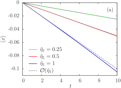
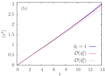
Figure 5: The first two moments of the numerical solutions of (6) (solid lines), $\langle x\rangle$ in part (a) and $\langle x^{2}\rangle$ in (b), are compared with the leading order contributions to the approximations given by (22a) respectively (22b) (dashed lines) for a linear viscosity profile $\eta(x)=\eta_{0}+\tilde{\eta}_{1}x$ with $\eta_{0}=10$ and different values of $\tilde{\eta}_{1}=0.25,~{}0.5,~{}1$.

The diffusion in an asymmetric viscosity profile (8) becomes anomalous too, as indicated by the contributions $\propto t^{2}$ and $\propto t^{3}$ to the approximate second moment in equation (22b). Again, the deviations are small between the full numerical result of $\langle x^{2}(t)\rangle$ [solid line in figure 5(b)] and the approximation (22b) [dashed line in figure 5(b)]. We point out, that anomalous diffusion still persists, when the drift of $\langle x\rangle$ is subtracted from the particle dynamics as illustrated by the following formula: $\langle x^{2}\rangle-\langle x\rangle^{2}=\frac{2\tilde{D}}{\eta_{0}}~{}t+\frac{\tilde{\eta}_{1}^{2}\tilde{D}^{2}}{\eta_{0}^{4}}~{}t^{2}+{\cal O}(\tilde{\eta}_{1}^{4})$. With the help of the third moment (22c) one can also define the skewness $S$ of a probability distribution [8], which is given in our case at the leading order by $S=-(3\tilde{\eta}_{1}\sqrt{\tilde{D}t})/(\sqrt{2}\eta_{0}^{3/2})$. Since $S$ is negative for $\tilde{\eta}_{1}>0$, the left tail of the probability distribution becomes more important.

All three aspects, the non-vanishing drift, the skewness of the particle distribution and the anomalous diffusion caused by an asymmetric monotonous viscosity profile are recaptured in numerical solutions of the Langevin equation (2) and the Fokker-Planck equation (6) by integrating both for the viscosity (7) up to time scales beyond the validity range of equations (22a)-(22c). The asymmetry of the resulting probability distribution is shown in figure 6(a) for increasing values of $\Delta\eta$, where the left tail is the more important one as predicted by the skewness $S$ of the distribution introduced above.

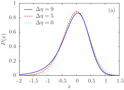
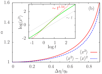
Figure 6: The probability distribution $P(x)$ at $t=1$ in (a) and the mean square displacement $\langle x^{2}\rangle$ in (b) are obtained by integrating (6) for the asymmetric viscosity (7) with $\eta_{0}=10$ and different values of $\Delta\eta=0,~{}5,~{}9$. The inset in (b) shows the three regimes of $\langle x^{2}(t)\rangle$ for $\eta_{0}=10$ and $\Delta\eta=9$. In the intermediate regime II at the largest slope (dashed line) the scaling exponent $\alpha$ is determined by the fit $\langle x^{2}\rangle\propto t^{\alpha}$ to the numerical data. In (b) the resulting $\alpha$ in regime II is given as function of $\Delta\eta/\eta_{0}$: The red solid line belongs to the evolution of $\langle x^{2}\rangle$ and the dashed line to the variance $\langle x^{2}\rangle-\langle x\rangle^{2}$.

The time dependence of the mean square displacement $\langle x^{2}(t)\rangle$ is shown for the viscosity (7) by the inset in figure 6(b) for $L=1$, $\eta_{0}=10$ and $\Delta\eta=9$ and illustrates all three temporal diffusion regimes. During the early temporal regime I with $|x|\ll L$ and in the long time limit with $|x|\gg L$ (regime III) one has normal diffusion with the exponent $\alpha=1$ as indicated by the dotted lines in the inset of 6(b). In contrast, during the intermediate regime II with $|x|\simeq L$ one has superdiffusion with $\alpha=1.543>1$ as indicated by the dashed line. If the numerical data of the mean square displacement, obtained for $\eta_{0}=10$ and $\Delta\eta=9$, are fitted by $\langle x^{2}\rangle\propto t^{\alpha}$ in the range of its largest slope in regime II we find that $\alpha$ is independent of the length $L$ as indicated by the values $\alpha=1.538~{}(L=0.2)$, $\alpha=1.543~{}(L=1)$, and $\alpha=1.544~{}(L=5)$. However, the exponent $\alpha$ varies strongly as a function $\Delta\eta/\eta_{0}$ in figure 6(b). As predicted by the analytical expressions in (22a) and (22b) the mean square displacement $\langle x^{2}\rangle$ [see also figure 5(b)] and the variance $\langle x^{2}\rangle-\langle x\rangle^{2}$ show anomalous diffusion behavior as well. The solid line in figure 6(b) describes the exponent $\alpha$ of the mean square displacement and the lower lying dashed line is the exponent related to the variance $\langle x^{2}\rangle-\langle x\rangle^{2}$. For both quantities the exponent $\alpha$ may take even larger values in the limit $\Delta\eta/\eta_{0}\to 1$. The mean value $\langle x\rangle$ drifts also for the viscosity profile (7). For small values of $t$ and $x$ we find a perfect agreement with the linear time dependence given by the leading contribution in (22b), but its dependence becomes more complex in the range of larger values of $\Delta\eta$ and in the long-time limit.

5 Conclusions

We have identified three different diffusion regimes for mesoscopic Brownian particles in spatially varying viscosities, which were analyzed by three approaches: Firstly, by scaling arguments applied to the expression of the mean square displacement, secondly by simulations of the corresponding nonlinear Langevin equation (2), and thirdly by solving the related Fokker-Planck equation (6) either numerically or, in limiting cases, even analytically. For an ensemble of particles starting at a viscosity extremum a short regime of normal diffusion is found where the mean square displacement $\langle x^{2}\rangle\propto t^{\alpha}$ scales with the exponent $\alpha=1$. Beyond this regime Brownian particles experience considerable changes of the viscosity along their trajectories, which leads to anomalous diffusive motion in an intermediate temporal regime. Near a minimum of the viscosity the particle dynamics becomes subdiffusive with an exponent $\alpha<1$, whereas it becomes superdiffusive with $\alpha>1$ in the vicinity of viscosity maxima. In the long time limit, when the Brownian particles explore the whole range of a viscosity variation, as for instance described by (9) or for a periodically varying viscosity, the particles experience a mean viscosity and therefore normal diffusion is found.

In the intermediate anomalous diffusive regime the particles’ probability distribution is non-Gaussian. In the case of a viscosity minimum the particle distribution function is - compared to a Gaussian with the same second moment - reduced at its maximum, increased at intermediate distances from its maximum, and reduced again at large distances. The opposite happens near a maximum of the viscosity: The particle distribution function is enhanced at the starting point of the particles and reduced at intermediate distances from the initial position. For an ensemble of particles starting in the range of a linearly varying viscosity profile, which is asymmetric with respect to the starting point, one finds an asymmetric particle distribution reflecting itself in a non-vanishing skewness. In addition, the first moment of the distribution drifts as function of time into the direction of decreasing viscosity and the particles show superdiffusive behavior. However, superdiffusivity is only partly caused by the particle drift: The exponent of the superdiffusive motion reduces only slightly towards 1 when the mean drift is subtracted from the particle motion but still shows clearly superdiffusive behavior with $\alpha>1$.

The subdiffusive behavior in an intermediate regime in the neighborhood of a minimum of the particle damping shares similarities with the Brownian dynamics of a single segment of a flexible polymer, the so-called Rouse dynamics. Also in this case one has normal diffusion of the segments on a short as well as on a long time scale. In the intermediate range, where the mean square displacement of the segment is of the order of the polymer-coil diameter, one finds the subdiffusive behavior $\langle x^{2}\rangle\propto t^{1/2}$ [32].

In contrast to most of the well-known examples showing anomalous diffusion, one can imagine for systems suggested in this work both types of anomalous diffusion, sub- and superdiffusion. In photorheological materials [37], for example, either a maximum or a minimum of the viscosity as well as monotonously varying viscosities can be induced by an appropriate spatial variation of the illumination strength. In some binary mixtures the sign of the Soret effect changes as a function of the mean temperature of the mixture [46]. The two possible signs may be used to attract either the lower viscous component to the locally heated area or the higher viscous component. In glass forming polymer-mixtures the relation between the local composition and the viscosity can be a nonlinear function [39, 40]. Materials with strong variations of the local viscosity are especially favorable to observe anomalous diffusion, as discussed in this work.

Another interesting subject are heated particles in a binary fluid mixture, undergoing Brownian motion. An example are light absorbing particles in a transparent binary fluid-mixture with an upper miscibility gap such as for instance $n$-Butoxyethanol and water [44], where the temperature may be driven close to the transition temperature. The inhomogeneous temperature field around a particle sets in much faster than related changes of the concentration and the viscosity in the neighborhood of the particle, such that the Brownian particle experiences temporally its own induced viscosity variations. The delayed dynamics between temperature and viscosity field may lead to interesting memory effects that are also prone to cause anomalous diffusion and will be investigated in forthcoming work.

References

- [1] Einstein A 1905 Ann. Phys. 17 549
- [2] Dhont J K G 1996 An Introduction to dynamics of colloids (Elsevier, Amsterdam)
- [3] Risken H 1984 The Fokker-Planck Equation (Springer, Berlin)
- [4] Hänggi P and Marchesoni F 2005 Chaos 15 026101
- [5] Gardiner C W 2009 Stochastic Methods (Springer, Berlin)
- [6] Sokolov I M and Klafter J 2005 Chaos 15 026103
- [7] Sokolov I M and Klafter J 2005 Phys. World 18 29
- [8] Anomalous Transport: Foundations and Applications 2008 edited by Klages R, Radons G and Sokolov I M (VCH Wiley, Weinheim)
- [9] Metzler R and Klafter J 2000 Phys. Rep. 339 1
- [10] Scher H and Montroll E W 1975 Phys. Rev. B 12 2455
- [11] Chate H, Ginelli F, Gregoire G and Raynaud F 2008 Phys. Rev. E 77 4
- [12] Narayan V, Ramaswamy S and Menon N 2007 Science 317 105
- [13] Arcizet D, Meier B, Sackmann E, Rädler J O and Heinrich D 2008 Phys. Rev. Lett. 101 248103
- [14] Höfling F, Frey E and Franosch T 2008 Phys. Rev. Lett. 101 120605
- [15] Brockmann D, Hufnagel L and Geisel T 2006 Nature 439 462
- [16] Kosztolowicz T, Dworecki K and Mrowczynski S 2005 Phys. Rev. Lett. 94 170602
- [17] Golding I and Cox E C 2006 Phys. Rev. Lett. 96 098102
- [18] Banks D S and Fradin C 2005 Biophys. J. 89 2960
- [19] Wong I Y, Gardel M L, Reichmann D R, Weeks E R, Valentine M T, Bausch A R and Weitz D A 2004 Phys. Rev. Lett. 92 178101
- [20] Dieterich P, Klages R, Preuss R and Schwab A 2008 Proc. Nat. Acad. Sci. (USA) 105 459
- [21] Dentz M, Cortis A, Scher H and Berkowitz B 2004 Adv. Water Resources 27 155
- [22] Alonso S, Kapral R and Bär M 2009 Phys. Rev. Lett. 102 238302
- [23] Zimmermann W, Sesselberg M and Petruccione F 1993 Phys. Rev. E 48 2699; Zimmermann W, Painter B and Behringer R 1998 Eur. Phys. J. B 5 575
- [24] Sokolov I M, Schmidt G W and Sagues F 2006 Phys. Rev. E 73 031102
- [25] Hentschel H G E and Procaccia I 1984 Phys. Rev. A 29 1461
- [26] Isichenko M B 1992 Rev. Mod. Phys. 64 961
- [27] Viscek T, Czirók, Ben-Jacob E, Cohen I and Shochet O 1995 Phys. Rev. Lett. 75 1226
- [28] Schweitzer F, Tilch B and Ebeling W 1998 Phys. Rev. Lett. 80 5044
- [29] Lindner B 2007 New J. Phys. 9 136
- [30] Dunkel J and Hänggi P 2005 Phys. Rev. E 71 016124
- [31] Dan D and Jayannavar A M 2002 Phys. Rev. E 66 041106
- [32] de Gennes P G 1979 Scaling Concepts in Polymer Physics (Cornell Univ. Press, Ithaca NY)
- [33] Klimontovich Y L 1994 Statistical Theory of Open Systems (Kluwer, Dordrecht).
- [34] Sancho J M, Miguel M S and Dürr D 1982 J. Stat. Phys. 28 291
- [35] Meredith J C, Karim A and Amis E J 2002 MRS Bulletin 27 330
- [36] Hoogenboom R, Meier M A R and Schubert U S 2003 Macromol. Rapid Commun. 24 16
- [37] Ketner A M, Kumar R, Davies T S, Elder P W and Raghavan S R 2007 J. Am. Chem. Soc. 129 1553
- [38] de Groot S R and Mazur P 1984 Non-equilibrium Thermodynamics (Dover, New York)
- [39] Williams M L, Landel R F and Fery J D 1955 J. Am. Chem. Soc. 77 3701
- [40] Rauch J and Köhler W 2002 Phys. Rev. Lett. 88 195901
- [41] Enge W and Köhler W 2004 Phys. Chem. Chem. Phys. 6 2373
- [42] Voit A, Krekhov A and Köhler W 2007 Phys. Rev. E 76 011808
- [43] Köhler W, Krekhov A and Zimmermann W 2010 Adv. Polymer Sci. 227 145
- [44] Aizpiri A G, Monroy F, del Campo C, Rubio R G and Pena M D 1992 Chem. Phys. 165 31
- [45] Øksendal B 2003 Stochastic Differential Equations (Springer, Berlin)
- [46] Kio R, Wiegand S and Luettner-Strathmann J 2004 J. Chem. Phys. 121 3874