Generation of wakefields by whistlers in spin quantum magnetoplasmas

Abstract

The excitation of electrostatic wakefields in a magnetized spin quantum plasma by the classical as well as the spin-induced ponderomotive force (CPF and SPF, respectively) due to whistler waves is reported. The nonlinear dynamics of the whistlers and the wakefields is shown to be governed by a coupled set of nonlinear Schrödinger (NLS) and driven Boussinesq-like equations. It is found that the quantum force associated with the Bohm potential introduces two characteristic length scales, which lead to the excitation of multiple wakefields in a strongly magnetized dense plasma (with a typical magnetic field strength $B_{0}\gtrsim 10^{9}$ T and particle density $n_{0}\gtrsim 10^{36}$ m^-3), where the SPF strongly dominates over the CPF. In other regimes, namely $B_{0}\lesssim 10^{8}$ T and $\ n_{0}\lesssim 10^{35}$ m^-3, where the SPF is comparable to the CPF, a plasma wakefield can also be excited self-consistently with one characteristic length scale. Numerical results reveal that the wakefield amplitude is enhanced by the quantum tunneling effect, however it is lowered by the external magnetic field. Under appropriate conditions, the wakefields can maintain high coherence over multiple plasma wavelengths and thereby accelerate electrons to extremely high energies. The results could be useful for particle acceleration at short scales, i.e. at nano- and micrometer scales, in magnetized dense plasmas where the driver is the whistler wave instead of a laser or a particle beam.

LABEL:FirstPage1 LABEL:LastPage#1102

I Introduction

Lately, significant progress has been made in the field of collective plasma accelerators for attaining high electron energies ProtonDrivenWake ; MultipleWake ; Wake-E-P-I1 ; Wake1 ; MagnetowaveWake ; Wake-E-P-I2 ; Wake2 ; Wake3 ; Wake4 ; WakeMagnetized ; WakeLaser . As is wellknown, an intense electromagnetic (EM) pulse can create a wake of plasma oscillations under the action of ponderomotive force WakeLaser . Electrons are then trapped into the wake and can thus be accelerated to extremely high energies, as high as giga- to teraelectronvolt scales. The idea that was presented by Tajima and Dawson WakeLaser three decades ago, has now become a reality through their experimental verifications RamanInstability ; BeatWave . Using intense laser beams or bunches of relativistic electrons have been used to excite plasma waves and to produce high electric field strengths (10-100 GV/m), opening up the possibility for compact GeV particle accelerators (see, e.g., ProtonDrivenWake for a discussion). Recently, an alternative scheme has been proposed for accelerating electrons up to the TeV regime, using proton bunches for driving plasma-wakefield accelerators ProtonDrivenWake .

A question that naturally arises is whether or not there exist natural (high-energy) systems, such as astrophysical environments, in which wakefield acceleration can take place. It is certainly true that neither high-intensity lasers, ultra-short photon bunches, or particle beams, used to excite wakefields in the laboratory regime, are readily available in the astrophysical settings, especially in dense plasmas characterizing, e.g., the interior of white dwarfs and Jovian planets. In contrast to the above examples of typical drivers, that may exist independent of a plasma medium, EM whistler waves only exist in a plasma environment. In this manner, Chen et al. Magnetowave2002 demonstrated the possibility of exciting large amplitude plasma wakefields by plasma magneto-waves, abundant in astrophysical settings. Later, particle-in-cell simulation has shown that this mechanism could well be valid for celestial acceleration MagnetowaveWake . However, no attempt has been made to generate wakefields self-consistently by whistler waves in strongly magnetized dense quantum plasmas with or without intrinsic spin of electrons.

On the other hand, dense electron plasmas are degenerate, and one must therefore take into account Fermi-Dirac statistics as well as tunneling effects PhysUsp . Furthermore, apart from the statistical effects introduced by the spin-$1/2$ nature of the electrons, the spin also generates a “dynamical” contribution, in the form of a pressure-like spin force and a spin magnetization current Spin-Nat ; Spin . The latter can even be larger than the classical free current when low-frequency (lf) longitudinal perturbations are driven by a spin-induced ponderomotive nonlinearity in the propagation of a short EM pulse SPF . Naturally, the inclusion of the quantum statistical pressure, the quantum force associated with the Bohm potential as well as the spin force due to finite magnetic moment of electrons in the dynamical equations, will significantly change the collective behavior of the electrons. For example, the Bohm potential, arising due to the particle’s wave-like nature, provides higher-order dispersion as well as the possibility of short-wavelength (compared to the electron skin depth) wakefield. The spin magnetization contributes to linear dispersion of circularly polarized modes JPPMisra and the magnetic dipole force results in a spin contribution to the ponderomotive force SPF .

In this paper, we present a theoretical investigation of the excitation of multiple wakefields driven by both the classical (CPF) CPF as well as the spin ponderomotive force (SPF) SPF of EM whistlers in a magnetized quantum plasma with intrinsic magnetization. The self-consistent fields of the whistlers and the wake are described by a coupled set of nonlinear Schrödinger- and modified Boussinesq-like equations WhistlerSpin . It is shown that when the SPF is comparable to CPF, the wakefields can be generated in the regime of strong magnetic fields with $B_{0}\lesssim 10^{8}$T and high-density plasmas with $\ n_{0}\lesssim 10^{35}$m${}^{-3}.$ However, multiple wakefields are also excited when the SPF dominates over the CPF in the very strongly magnetized and superdense plasmas with $B_{0}\gtrsim 10^{9}$T, $n_{0}\gtrsim 10^{36}$m${}^{-3}.$ In the latter, the results of our model is that the whistler wavelength may be even shorter than the Compton wavelength of the electrons. This gives rise to a viable mechanism for wakefield acceleration in spin dominated plasmas, such as those in superdense astrophysical bodies, e.g., white dwarfs, neutron stars, magnetars.

II Evolution equations

We consider the propagation of high-frequency (hf) whistler waves along an external magnetic field $\mathbf{B}=B_{0}\hat{z}$ in a quantum plasma, taking into account the intrinsic spin of the electrons. The heavy ions are assumed to be immobile, so that the lf density response occurs on a time-scale much shorter than the ion plasma period. In the modulational representation, the whistler electric field can be represented by $\mathbf{E}=\left(\hat{x}-i\hat{y}\right)E(z,t)\exp(ikz-i\omega t)+$c.c., where $E(z,t)$ is the slowly varying wave envelope, $\omega$ ($k$) is the whistler wave frequency (number) and c.c. stands for the complex conjugate. Then the basic equations for the evolution of whistlers consist of the fluid equations for the nonrelativistic evolution of spin$-1/2$ electrons given by Spin ; WhistlerSpin

$$\partial_{t}n_{e}+\nabla.\left(n_{e}\mathbf{v}_{e}\right)=0$$ (1)

$$\left(\partial_{t}+\mathbf{v}_{e}.\nabla\right)\mathbf{v}_{e} =-\frac{e}{m_{e}}\left(\mathbf{E}+\mathbf{v}_{e}\times\mathbf{B}\right)-\frac{\nabla P_{e}}{m_{e}n_{e}}$$

$$\quad+\frac{\hbar^{2}}{2m_{e}^{2}}\nabla\left(\frac{\nabla^{2}\sqrt{n_{e}}}{\sqrt{n_{e}}}\right)+\frac{2\mu}{m_{e}\hbar}\mathbf{S}.\nabla B$$ (2)

$$\left(\partial_{t}+\mathbf{v}_{e}.\nabla\right)\mathbf{S}=-\left(2\mu/\hbar\right)\left(\mathbf{B}\times\mathbf{S}\right),$$ (3)

and the Maxwell equations for the electromagnetic (EM) fields

$$\nabla\times\mathbf{E}=-\partial_{t}\mathbf{B},\text{ }\nabla.\mathbf{B}=0$$ (4)

$$\nabla\times\mathbf{B}=\mu_{0}\left(\varepsilon_{0}\frac{\partial\mathbf{E}}{\partial t}\mathbf{-}en_{e}\mathbf{v}_{e}\mathbf{+}\frac{2\mu}{\hbar}\nabla\times n_{e}\mathbf{S}\right).$$ (5)

Here $n_{e},$ $m_{e},$ $\mathbf{v}_{e}$ denote the number density, mass and velocity of electrons respectively, $\mathbf{B}$ is the magnetic field and $P_{e}$ is the electron thermal pressure and $\mathbf{S}$ is the spin angular momentum with $\left|\mathbf{S}\right|=\left|S_{0}\right|\equiv\hbar/2,$ $\mu=-\left(g/2\right)\mu_{B},$where $g\approx 2.0023193$ is the electron $g$-factor and $\mu_{B}\equiv e\hbar/2m_{e}$ is the Bohr magneton. The equations (1)-(3) are applicable even when different spin states (with up and down) are well represented by a macroscopic average. This may, however, occur in the regimes of very strong magnetic fields (or a very low temperature plasmas), where generally the electrons occupy the lowest energy spin states. On the other hand, for a time-scale larger than the spin-flip frequency, the macroscopic spin state (to be attenuated by a factor decreasing the effective value of $\left|\mathbf{S}\right|$ below $\hbar/2$) can  be well-described by the thermodynamic equilibrium spin configuration, and in this case the above fluid model can still be applied. However, this is not the present issue to be studied here rather we will focus on the regimes of strong magnetic fields and high density plasmas.

The evolution equation for the whistler can be obtained by taking the curl of Eq. (2) [hence the pressure gradient and the quantum force in Eq. (2) vanish] and using Eqs. (3)-(5) as

$$0 =\frac{e}{m_{e}}\frac{\partial\mathbf{B}}{\partial t}+\frac{\varepsilon_{0}}{en_{e}}\frac{\partial}{\partial t}\left(\frac{\partial^{2}\mathbf{B}}{\partial t^{2}}+\frac{1}{n_{e}}\nabla n_{e}\times\frac{\partial\mathbf{E}}{\partial t}\right)-v_{ez}\nabla\times\frac{\partial\mathbf{v}_{e}}{\partial z}+\frac{1}{e\mu_{0}}\frac{\partial}{\partial t}\left[\frac{1}{n_{e}}\nabla\times\left(\nabla\times\mathbf{B}\right)\right]$$

$$-\frac{2\mu}{e\hbar}\frac{\partial}{\partial t}\left[\frac{1}{n_{e}}\nabla\times\left(\nabla\times n_{e}\mathbf{S}\right)\right]+\frac{1}{m_{e}\mu_{0}n_{e}}\nabla\times\left[\left(\nabla\times\mathbf{B}\right)\times\mathbf{B}\right]+\frac{2\mu}{m_{e}\hbar}\nabla\times\left(S^{a}\nabla B_{a}\right)$$

$$-\frac{\varepsilon_{0}}{m_{e}n_{e}}\nabla\times\left(\frac{\partial\mathbf{E}}{\partial t}\times\mathbf{B}\right)-\frac{2\mu}{m_{e}\hbar n_{e}}\nabla\times\left[\left(\nabla\times n_{e}\mathbf{S}\right)\times\mathbf{B}\right].$$ (6)

We note that in the nonlinear interaction of hf EM waves with the lf electron plasma response, the use of cold plasma approximation is also justified to the fact that for large field intensities and moderate electron temperature, the directed speed of electrons in the hf fields is much larger than the random thermal speed. It can also be shown that the density perturbation associated with the hf EM wave is zero. Thus, the evolution equation (6) for the whistlers do not involve contributions from the electron pressure and the quantum tunneling effect proportional to $\hbar^{2}$. Later, we will see that these contributions will appear in the coupling of the lf plasma response with the hf one through the ponderomotive force induced by the hf field.

Introducing the variables $B_{\pm}=B_{x}\pm iB_{y},$ $E_{\pm}=E_{x}\pm iE_{y}$ etc., suitable for circularly polarized waves, and linearizing we obtain respectively from the Faraday’s law and the spin-evolution equation (13) as SPF

$$B_{\pm}=\pm\frac{ik}{\omega}E_{\pm},\text{ }S_{\pm}=\mp\frac{2\mu\left|S_{0}\right|B_{\pm}}{\hbar\left(\omega\pm\omega_{g}\right)}$$ (7)

We then linearize Eq. (6) and use Eq. (7) to obtain the following linear dispersion relation for the circularly polarized modes JPPMisra

$$n_{R}^{2}=1-\frac{\omega_{pe}^{2}}{\omega\left(\omega\pm\omega_{c}\right)}-\frac{g^{2}\omega_{pe}^{2}k^{2}\left|S_{0}\right|}{4\omega^{2}m_{e}\left(\omega\pm\omega_{g}\right)},$$ (8)

which can be rewritten as

$$n_{R}^{2}\left(1+\frac{\omega_{\mu}}{\omega-\omega_{g}}\right)=1-\frac{\omega_{pe}^{2}}{\omega\left(\omega-\omega_{c}\right)},$$ (9)

where $n_{R}\equiv ck/\omega$ is the refractive index, $\omega_{\mu}=g^{2}\left|S_{0}\right|/4m_{e}\lambda_{e}^{2}$ is the frequency due to the plasma magnetization current and $\lambda_{e}\equiv c/\omega_{pe}$ is the electron skin depth with $\omega_{pe}\equiv\sqrt{n_{0}e^{2}/\varepsilon_{0}m_{e}}$ denoting the electron plasma frequency. Moreover, $\omega_{c}=eB_{0}/m_{e}\$is the electron-cyclotron frequency and $\omega_{g}=(g/2)\omega_{c}$  is the electron spin-precession frequency. We note that the frequency resonances occur not only at the cyclotron frequency ($\omega\rightarrow\omega_{c}$) but also due to the spin-gyration of electrons ($\omega\rightarrow\omega_{g}$), although these resonances are close to each other. At the resonance, the transverse field associated with the whistlers rotates at the same speed as electrons gyrates around the external magnetic field. The electrons will then experience a continuous acceleration from the wave electric field. However, the detail discussion on the properties of the linear modes modified by the spin magnetization current can be found in the literature JPPMisra . One can see that when $\omega_{c}\gg\omega_{pe},$ i.e., the magnetic field is strong enough, but $\omega_{\mu}$ is still smaller than $\omega_{pe}$ (unless we consider a very high-density regime), the dispersion of the whistler wave are almost linear (with phase speed approaching the speed $c$ of light in vacuum$)$ over a wide range of wave numbers. However, it may remain nonlinear in strongly magnetized high density plasmas depending on the parameter regimes we consider JPPMisra . This nonlinear behaviors of whistlers in which $E,$ $B$ wave fields are not comparable in strength do not favor the excitation of wakefields, and we do not consider those cases here.

On the other hand, in the nonlinear regime, the dynamics of whistler wave envelopes can be described from Eq. (6) by the following nonlinear Schrödinger (NLS)-like equation WhistlerSpin .

$$i\left(\partial_{t}E+v_{g}\partial_{z}E\right)+\left(v_{g}^{\prime}/2\right)\partial_{z}^{2}E-\Delta E=0,$$ (10)

where $E\equiv E_{x}-iE_{y},$ $v_{g}\equiv d\omega/dk$  is the group speed, $v_{g}^{\prime}\equiv d^{2}\omega/dk^{2}$ is the group dispersion of whistlers and $\Delta$ is the nonlinear frequency shift. These are given by WhistlerSpin

$$v_{g}=\left(\frac{2c^{2}k}{\omega_{pe}^{2}}+\frac{g^{2}\hbar k}{4m_{e}\left(\omega-\omega_{g}\right)}\right)/\left(\frac{2\omega}{\omega_{pe}^{2}}+\frac{\omega_{c}}{\left(\omega-\omega_{c}\right)^{2}}+\frac{g^{2}\hbar k^{2}}{8m_{e}\left(\omega-\omega_{g}\right)^{2}}\right),$$ (11)

$$v_{g}^{\prime}=\frac{v_{g}}{k}\left[1-\frac{2kv_{g}^{2}}{\Lambda\omega_{pe}^{2}}\left(1-\frac{\omega_{c}\omega_{pe}^{2}}{\left(\omega-\omega_{c}\right)^{3}}\right)-\frac{g^{2}\hbar k^{2}v_{g}}{4m_{e}\Lambda\left(\omega-\omega_{g}\right)^{2}}\left(2-\frac{v_{g}k}{\omega-\omega_{g}}\right)\right],$$ (12)

and

$$\Delta=\frac{v_{g}}{\Lambda}\left[\frac{k\omega v_{ez}}{\left(\omega-\omega_{c}\right)^{2}}+\left(\frac{\omega}{\omega-\omega_{c}}+\frac{g^{2}\hbar k^{2}}{4m_{e}\left(\omega-\omega_{g}\right)}\right)N\right],$$ (13)

where $\Lambda=2c^{2}k/\omega_{pe}^{2}+g^{2}\hbar k/4m_{e}\left(\omega-\omega_{g}\right),$ $N\equiv n_{e}/n_{0}$ and $v_{ez}$ is the magnetic field aligned free electron flow speed.

Note that the variables $v_{ez}$ and $N$ appear due to the lf electron plasma response, and are to be coupled with hf field through the ponderomotive force. The governing equations for the nonlinear coupling of these two responses will be described later. Furthermore, in Eqs. (11)-(13), the terms proportional to $\hbar$ are contributions from the plasma magnetization current due to intrinsic spin of electrons. Notice, however, that when the spin effects dominate, the group velocity tends to decrease as the frequency of the whistler approaches the cyclotron frequency  JPPMisra and/ or $k$ increases its value. The latter indicates a negative group dispersion in the propagation of whistlers. Notice, however, that the nonlinear frequency shift precisely depends on the group velocity, and can even become larger (when $\omega$ approaches $\omega_{c})$ due to the plasma streaming with the flow speed $v_{ez}$ along the external magnetic field.

Let us now compare the two ponderomotive forces, which induce slowly varying electrostatic oscillations in plasmas. The expressions of these forces, namely CPF CPF and SPF SPF [Note that in the expression for the spin ponderomotive force given by Eqs. (12) and (13) in Ref. SPF , a factor $2$ was missing in the denominator, and this factor $2$ appears in the average of the forces as in Eqs. (7) and (8) there for the classical part] acting on an individual electron can be written respectively as

$$F_{cz}=-\frac{1}{2}\frac{e^{2}}{m_{e}^{2}\omega\left(\omega-\omega_{c}\right)}\left(1+\frac{\omega_{c}}{\omega}\frac{kv_{g}}{\omega-\omega_{c}}\right)\frac{\partial\left|E\right|^{2}}{\partial\xi},$$ (14)

$$F_{sz}=-\frac{1}{4}\left(\frac{g^{2}\hbar k^{2}}{4m_{e}\omega}\right)\frac{e^{2}}{m_{e}^{2}\omega\left(\omega-\omega_{g}\right)}\left(1+\frac{kv_{g}}{\omega-\omega_{g}}\right)\frac{\partial\left|E\right|^{2}}{\partial\xi},$$ (15)

where $\xi=z-v_{g}t$ is the co-moving frame of reference for the driving whistler. The spin induced ponderomotive force arises due to the effects of the finite magnetic moment of electrons and is obtained by taking the average over the fast time scale of the spin force in the momentum equation (2) SPF . We note that the spin contribution to the ponderomotive force is small compared to the classical one when the factor $\chi\equiv$ $\hbar k^{2}/m_{e}\omega\ll 1.$ In this case, one can typically neglect the spin-contribution in the linear as well as nonlinear regimes, and thus the results will be valid for weakly or strongly magnetized low-density plasmas. However, for an exception to this rule, see Ref. SPF . In the opposite limit, i.e.,  $\chi\gg 1,$ the SPF in Eq. (15) can, indeed, dominate over the CPF when the whistler wave frequency is close to the cyclotron frequency. In this case, the whistler (with phase speed close to $c)$ wavelength $\left(\lambda_{W}=2\pi/k\right)$ can be smaller or of the order of the Compton wavelength $\left(\lambda_{C}=h/mc\right)$ of electrons, since $\hbar k^{2}/m_{e}\omega\$scales as $\lambda_{C}/\lambda_{W}$. This case can be relevant in  very strongly magnetized ($B_{0}\gtrsim 10^{9}$T) and very high-density medium ($n_{0}\gtrsim 10^{36}$m${}^{-3})$ in which $\omega_{c}>\omega_{pe}$ still holds. The whistler wave dispersion can then still be linear and the group as well the phase speed of the whistlers may approach   the speed of light in vacuum. Below, we will see that this is the case in which the whistler pulses can maintain their shape over a macroscopic distance, and thus favors the plasma wakefield acceleration.

Next, the whistler dispersion may be linear in the regimes of $B_{0}\sim 10^{8}$ T and $n_{0}\sim 10^{35}$ m^-3 where the SPF may not be dominant over, but may be comparable to the CPF $F_{cz}$. On the other hand, for $\omega\ll\omega_{c}$ and $\chi\gg 1,$ though the first term in the square brackets in Eq. (14) is negligible, but the second one can not be so, rather may be comparable to the spin contribution. In this case, ion dynamics might play roles, and also the whistler wavelength may be much larger than the plasma characteristic length scale. So, this case will not be so effective for high energy particle acceleration. We will focus on the regimes as discussed above for which the excitation of multiple wakefields is possible. For $\omega\gg\omega_{c}$ and $\chi\gg 1,$ the classical part is also negligible, however, this is not relevant  to the present study.

The equations for the lf density response which arises due to the ponderomotive force of the hf electromagnetic field satisfy the electron continuity, momentum balance and the Poisson equation, these are respectively

$$\partial_{t}N+\partial_{z}v_{ez}=0.$$ (16)

$$\partial_{t}v_{ez}+\frac{e}{m_{e}}E_{l}+V_{F}^{2}\partial_{z}N-\left(\hbar^{2}/4m_{e}^{2}\right)\partial_{z}^{3}N$$

$$=\frac{e^{2}}{2m_{e}^{2}\omega^{2}}\left(\Gamma_{1}\partial_{z}|E|^{2}-k\Gamma_{2}\partial_{t}|E|^{2}\right),$$ (17)

$$\partial_{z}E_{l}=\frac{e}{\varepsilon_{0}}(n_{0}-n_{e}),$$ (18)

where $E_{l}$ is the lf part of the wave electric field (wakefield) and $V_{F}$ $=\sqrt{k_{B}T_{F}/m_{e}}$  is the Fermi speed relevant for a low-temperature high density plasmas FermiPressure , $T_{F}\equiv\hbar^{2}\left(3\pi^{2}n_{0}\right)^{2/3}/2k_{B}m_{e}$ is the Fermi temperature with $k_{B}$ denoting the Boltzmann constant. The term $\propto\hbar^{2}$ is the effect of quantum tunneling associated with the Bohm de Broglie potential. The ponderomotive force contributions are proportional to the constants $\Gamma_{1}$ and $\Gamma_{2}$  WhistlerSpin where

$$\Gamma_{1} =\frac{\omega}{\omega-\omega_{c}}+\frac{g^{2}\hbar k^{2}}{8m_{e}\left(\omega-\omega_{g}\right)},$$

$$\Gamma_{2} =\frac{\omega_{c}}{\left(\omega-\omega_{c}\right)^{2}}+\frac{g^{2}\hbar k^{2}}{8m_{e}\left(\omega-\omega_{g}\right)^{2}},$$ (19)

in which the first terms appear due to CPF CPF and the second $\left(\propto\hbar\right)$ are due to the SPF SPF .  From Eq. (19) we note that for $\chi\gg 1,$ the SPF contribution is substantial compared to the CPF, and $\Gamma_{1,2}$ can be approximated as $\propto\hbar$ that represents purely a spin quantum effect. Equations (16)-(18) can be combined to obtain the driven wave equation for lf perturbations of the Boussinesq-type

$$\left[\partial_{t}^{2}+\frac{\hbar^{2}}{4m_{e}^{2}}\partial_{z}^{4}-V_{F}^{2}\partial_{z}^{2}+\omega_{pe}^{2}\right]N=\mu_{1}\partial_{z}^{2}|E|^{2}-\mu_{2}\partial_{zt}^{2}|E|^{2},$$ (20)

where the ponderomotive force contributions are $\mu_{1}=\varepsilon_{0}\omega_{pe}^{2}\Gamma_{1}/2m_{e}\omega^{2}\$and $\mu_{2}=\varepsilon_{0}\omega_{pe}^{2}k\Gamma_{2}/2m_{e}\omega^{2}$ in which spin effect is hidden.

Thus, we have a new set of three coupled equations, namely (10), (16) and (20), modified by the SPF and the effect of quantum tunneling, which describes the nonlinear coupling of electron whistlers with the field aligned electrostatic density fluctuations. These equations can be written in the nondimensional forms as ($z\rightarrow z/\lambda_{Fe},t\rightarrow t\omega_{pe},E\rightarrow E/E_{0},$ $v_{ez}\rightarrow v_{ez}/c_{s}$, where $\lambda_{Fe}=V_{F}/\omega_{pe}=\lambda_{e}V_{F}/c$)

$$i\left(\partial_{t}E+V_{g}\partial_{z}E\right)+\left(V_{g}^{\prime}/2\right)\partial_{z}^{2}E-\Psi E=0,$$ (21)

$$\partial_{t}N+\partial_{z}v_{ez}=0,$$ (22)

$$\left[\partial_{t}^{2}+H^{2}\partial_{z}^{4}-\partial_{z}^{2}+1\right]N=\zeta_{1}\partial_{z}^{2}|E|^{2}-\zeta_{2}\partial_{zt}^{2}|E|^{2},$$ (23)

where $E_{0}=\sqrt{2k_{B}T_{F}n_{0}/\varepsilon_{0}},$ $V_{g}=v_{g}/V_{F},V_{g}^{\prime}=v_{g}^{\prime}\omega_{pe}/V_{T}^{2},$ $\Psi=\Delta/\omega_{pe},$ $H=\hbar\omega_{pe}/2k_{B}T_{F}$  is the quantum parameter and $\zeta_{1}=\omega_{pe}^{2}\Gamma_{1}/\omega^{2},$ $\zeta_{2}=\omega_{pe}^{2}kV_{F}\Gamma_{2}/\omega^{2}.$ Equations (21)-(23) contain the main results of the present work.

III Excitation of the wakefields

In this section, we consider the excitation of one-dimensional wakefield by the hf whistlers propagating with the group velocity. Thus, we look for stationary solutions of our main Eqs. (21)- (23) in the frame $\xi=z-V_{g}t$. To this end, we assume $E$ to be of the form $E=W\left(\xi\right)\exp\left(-i\Theta t\right),$ where $\ W$ is a real function normalized by $E_{0}$ and $\Theta$ is a real constant. Then Eqs. (21)- (23) reduce to

$$\left(V_{g}^{\prime}/2\right)d_{\xi}^{2}W+W\Omega-\tilde{\Delta}NW=0,$$ (24)

$$\left[H^{2}d_{\xi}^{4}+\left(V_{g}^{2}-1\right)d_{\xi}^{2}+1\right]N=\left(\zeta_{1}+\zeta_{2}V_{g}\right)d_{\xi}^{2}W^{2},$$ (25)

where

$$\tilde{\Delta}=\frac{v_{g}}{\Lambda\omega_{pe}}\frac{\omega}{\omega-\omega_{c}}\left(1+\frac{kv_{g}}{\omega-\omega_{c}}+\frac{g^{2}\hbar k^{2}}{4m_{e}\omega}\frac{\omega-\omega_{c}}{\omega-\omega_{g}}\right).$$ (26)

Equation (25) shows that the electrostatic wake field is created by the self-consistent whistler waves.  We also find that the inclusion of the quantum correction $\propto H$ leads to two different characteristic length scales, which, in turn, will give rise multiple oscillatory wakefields. Thus, considering a trial solution of the corresponding homogeneous equation of (25) as $N\sim\exp(ik_{p}\xi),$ we obtain $k_{p}^{4}-\kappa_{a}^{2}k_{p}^{2}+\kappa_{b}^{4}=0,$ where $\kappa_{a}=(V_{g}^{2}-1)^{1/2}/H\$ and $\ \kappa_{b}=1/\sqrt{H}.$ This biquadratic equation has, in general, two pairs of real roots $\pm k_{1,2}$ MultipleWake for $V_{g}\equiv v_{g}/V_{F}>\sqrt{1+2H}$ where

$$k_{1,2}^{2}=\frac{\kappa_{a}^{2}}{2}\mp\sqrt{\frac{\kappa_{a}^{4}}{4}-\kappa_{b}^{4}}.$$ (27)

For a Gaussian driving pulse of the form $W\sim\exp\left(-\xi^{2}/L_{p}^{2}\right),$ Eq. (25) yields the wakefield behind the driving pulse, i.e., for $\left|\xi\right|\gg L_{p}$ as $N=N_{2}-N_{1}$ where

$$N_{1,2}\approx\frac{4\kappa_{b}^{4}\left(\zeta_{1}+\zeta_{2}V_{g}\right)}{\left(12-L_{p}^{2}k_{1,2}^{2}\right)\left(k_{2}^{2}-k_{1}^{2}\right)}\cos\left(k_{1,2}\xi\right)$$ (28)

and, in particular, in absence of the quantum force,

$$N\approx\frac{4\kappa_{p}^{2}\left(\zeta_{1}+\zeta_{2}V_{g}\right)}{\left(12-L_{p}^{2}k_{p}^{2}\right)}\cos\left(\kappa_{p}\xi\right),$$ (29)

where $\kappa_{p}=1/(V_{g}^{2}-1)^{1/2}.$

Next, for the generation of whistler driven wakefields, we numerically solve the Eqs. (24) and (25) by Newton’s method with the boundary conditions $N$, $W$, $dN/d\xi,$ $dW/d\xi\rightarrow 0$ as $\xi\rightarrow\pm\infty.$ In order to study the influence of the quantum tunneling effect, we consider two cases, namely for $H=0$ [Note, however, that $H$ $\left(\sim 1/\hbar\right)=0$ does not mean that one recovers the $\hbar=0$ case, rather it implies that we have simply disregarded the quantum tunneling effect associated with the Bohm potential] and for nonzero $H.$ Here the typical length scale for plasma collective oscillation is the Fermi screening length $\lambda_{Fe}=\lambda_{e}V_{F}/c<\lambda_{e}$ as long as the $V_{F}<c,$ and it must be such that $\lambda_{Fe}<\lambda_{W},$ the whistler wavelength. The typical time scale is the electron plasma period, which is shorter than the ion plasma period for which the ion dynamics is negligible.  Moreover, quantum effects become important when $\zeta\equiv T_{F}/T_{classical}=\left(1/2\right)\left(3\pi^{2}n_{0}\lambda_{B}^{3}\right)^{2/3}\gtrsim 1,$ where $\lambda_{B}=\hbar/m_{e}V_{F}$ is the thermal de Broglie wavelength. Furthermore, the quantum coupling parameter $g_{Q}\sim\left(1/n_{0}\lambda_{Fe}^{3}\right)^{2/3}\lesssim 1$ defines a quantum collisionless regime where the collective and mean-field effects dominate. We now study the two cases as follows.

In the case of $H=0$, the plasma characteristic length scale for the wake is $\lambda_{p}=2\pi/\kappa_{p},$ and we choose the parameters as $B_{0}=3\times 10^{8}$ T, $n_{0}=10^{35}$ m^-3 and $\omega=0.78,$ $\Theta=0.22,$ for which $\omega/\omega_{p}=2.3,$ $\omega_{c}/\omega_{p}=3,v_{g}/V_{F}=1.3,v_{g}/v_{p}=0.7,$ $\lambda_{Fe}/\lambda_{e}=0.4$ and $E_{0}=1.7\times 10^{16}$V/m. In this case the plasma oscillation length is $\lambda_{p}(=5.4)>\lambda_{W}$ $(\equiv 2\pi/k\lambda_{Fe}$ in normalized form$)=5.3,$ the group   dispersion $V_{g}^{\prime}=-2.7$ and the nonlinear frequency shift $\tilde{\Delta}=0.4.$ Moreover, $g_{Q}=0.11<1$ and $\zeta\sim 1.$ Thus, in the quantum regime, the short-scale wakefield can be generated as shown in the upper panel of Fig. 1.  Increasing the magnetic field strength, namely $B_{0}=6\times 10^{8}$ T and keeping electron concentration as the same, i.e., $n_{0}=10^{35}$ m^-3, we find that the group velocity increases ($v_{g}/v_{p}=0.85$) and hence for a increasing value of the ratio $\omega_{c}/\omega_{p}=5.9,$ the wakefield remains coherent, but its amplitude becomes much lowered (not shown in the figure).  The whistler group dispersion has now been lowered as $V_{g}^{\prime}=-1.5$ than the previous case and the frequency is shifted-up to $\tilde{\Delta}=0.53$. The other parameter values in this regime are, e.g., $\lambda_{p}=10.9$ and $\lambda_{W}=3.2.$

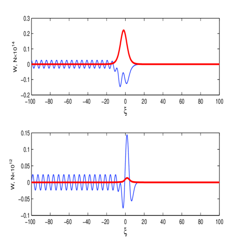
Figure 1: (Color online) Plasma wakefields [Numerical solution of Eqs. (24) and (25)] driven by the whistlers (thick line) for $H=0$ (upper panel) and for $H=0.13$ (lower panel) with characteristic length scales $\lambda_{p}=5.4$ $(\lambda_{Fe})$ and  $\lambda_{1}=5.5$ $(\lambda_{Fe})$ respectively. The case in which SPF is comparable to CPF. The parameter values are given in the text.

The lower panel of Fig. 1 shows the wakefields for a nonzero $H$.  We find that the plasma wake electric field is enhanced due to the quantum tunneling effect.  Here the corresponding plasma characteristic length scales are $\lambda_{1,2}=2\pi/$ $k_{1,2}$ as defined above. For the length scale $\lambda_{1},$ we use the parameters $B_{0}=6\times 10^{8}$ T, $n_{0}=2\times 10^{35}$ m${}^{-3},$ $\omega=0.78\$and $\Theta=0.04$ for which $\omega/\omega_{p}=3.3,$ $\omega_{c}/\omega_{p}=4.2,$ $v_{g}/V_{F}=1.3,$ $v_{g}/v_{p}=0.77,$ $k\lambda_{Fe}=1.9,$ $H=0.13,$ $\lambda_{1}=5.5,$ $\lambda_{W}=3.3,V_{g}^{\prime}=-1.5$ and $\tilde{\Delta}=0.5.$ We note that the length scale $\lambda_{2}$ does not favor the wakefield generation in the parameter regimes considered above, since for $V_{g}>\sqrt{1+2H},$ $\lambda_{2}$ scales as the Compton wavelength, which becomes lower than the whistler wavelength $\lambda_{W}$.  However, since as said before, $\lambda_{W}$ may approach or lower than the Compton wavelength in the case of very strongly magnetized and very high density plasmas where the SPF dominates over the CPF, multiple wakefield generation can be possible as can be illustrated from Fig. 2 below.

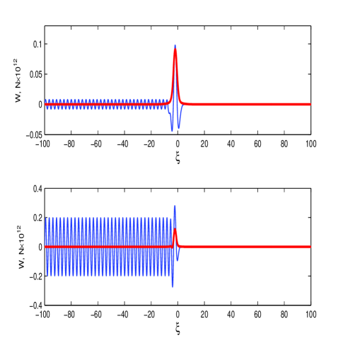
Figure 2: (Color online) Plasma wakefields [Numerical solution of Eqs. (24) and (25)] driven by the whistlers (thick line) for a fixed $H=0.13$ but for two different characteristic length scales $\lambda_{1}=2.8$ $(\lambda_{Fe})$ (upper panel) and $\lambda_{2}=1.45$ $(\lambda_{Fe})$ (lower panel). The case in which SPF dominates over CPF. The parameter values are given in the text.

Thus, for the parameters $B_{0}=4\times 10^{9}$ T, $n_{0}=10^{36}$ m^-3 and $\omega=0.78,$ $\Theta=0.008$ for which $\omega/\omega_{p}=9.7,$ $\omega_{c}/\omega_{p}=12.5,v_{g}/V_{F}=1.1,v_{g}/v_{p}=0.97,$ $k\lambda_{e}=9.97,$ $k\lambda_{Fe}=8.4,$ $2\pi/k\lambda_{e}=0.63,$ $H=0.13,$ $\lambda_{W}=0.75,V_{g}^{\prime}=-0.1,$ $\tilde{\Delta}=0.3,$ the corresponding wakefield excitation is shown in the upper panel of Fig. 2 with $\lambda_{1}=2.8.$ From the lower panel of this figure one can see the similar excitation but with a shorter scale $\lambda_{2}=1.45.$ In the latter, wakefield amplitude is seen to be enhanced compared to the case with $\lambda_{1}.$

IV Discussion and conclusion

Numerical results in the previous section suggest that wakefield excitation by the whistlers can be possible in a strongly magnetized dense plasmas ( $B_{0}\lesssim 10^{8}$ T and $\ n_{0}\lesssim 10^{35}$ m${}^{-3})$ with intrinsic spin of electrons. In this regime the SPF is no longer negligible rather may be comparable to the CPF. Such parameter regimes can be achievable in the interior of white dwarf stars where electrons are indeed degenerate and the electron degeneracy pressure is what supports a white dwarf against gravitational collapse. The magnetic fields in such compact degenerate stars might be due to conservation of total surface magnetic flux during the evolution or by the  emission of circularly polarized light or else. However, a small number of white dwarfs have been examined for magnetic field strength exceeding $10^{5}$ T.

In absence of the quantum force, the wakefields can be generated with the characteristic length scale $\lambda_{p}=2\pi(V_{g}^{2}-1)^{1/2}$ and in the parameter regimes $B_{0}\sim 10^{8}$ T, $\ n_{0}\sim 10^{35}$ m^-3 as described above. Apart from the Fermi pressure, the quantum tunneling effect associated with the Bohm potential introduces an additional higher-order dispersion. The latter, in turn, introduces two characteristic length scales $\lambda_{1}$ and $\lambda_{2}$ $\left(<\lambda_{1}\right)$ (quite distinctive from the case with $H=0$) out of which only $\lambda_{1}$ favors the wakefield excitation in the said regimes, since  $\lambda_{2}$ becomes smaller than the whistler wavelength $\lambda_{W}$ ($\gtrsim 10^{-12}$ m), a case not effective for the wakefield generation. However, multiple wakefield excitation can be possible with two length scales $\lambda_{1}$ and $\lambda_{2}$ in very strongly magnetized and superdense plasmas with $B_{0}\gtrsim 10^{9}$ T and $n_{0}\gtrsim 10^{36}$ m${}^{-3}.$ In these regimes the CPF is strongly dominated by the SPF.  The latter will then dominantly accelerate the electrons by separating the electric charges and building up a high electric field.  Furthermore, such parameter regimes could be relevant in the deeper layer (above the neutron-drip layer) of the crust of neutron star in which electrons are degenerate implying that electrical and thermal conductivity may be huge because the electrons can travel great distances before interacting. However,  the physics and the composition of neutron star interiors are not yet fully understood.

We ought to mention that in the regimes of very strong magnetic fields and superdense plasmas as mentioned above, the nonrelativistic fluid model may no longer be appropriate as in such cases the Fermi speed approaches (or can be greater than) the speed of light in vacuum and whistler wavelength may become smaller than the Compton wavelength of electrons. In this situation, relativistic spin-quantum fluid model or kinetic approach could be well set. By increasing the magnetic field strength or the ratio $\omega_{c}/\omega_{p},$ we see that whistler wave can have smaller group dispersion. This could be important for whistler waves to be a viable mechanism in magnetized dense plasmas in order to gain higher energy for an accelerated particle from the plasma wakefield.

Next, as an alternative mechanism instead of using lasers or particle beams as drivers which have been used mostly for laboratory plasma wakefield accelerations, the EM whistler waves should be of fundamental interest in plasmas, in particular, quantum plasmas for astrophysical settings. However, conclusive evidence needs further investigation in this area by considering, e.g., full scale simulation of a relativistic fluid model or kinetic one accounting for the quantum statistical and mechanical (tunneling) effects as well as intrinsic spin of electrons. The latter might have a role in the regimes previously considered to be as classical Spin-kinetic . We mention that our model can be well applicable for low or moderate density magnetized plasmas as well where electrons may not be degenerate, spin effects might not be so important. In this case one can consider, e.g., the isothermal equation of state instead of the Fermi pressure law for electrons.  Thus, classical results can also be recovered by disregarding the term $\propto\hbar$ for the spin contribution and the term $\propto\hbar^{2}$ for the quantum tunneling effect.

To mention, neutron stars are known to be compact and carry intense surface magnetic fields   about $10^{9}$ T or more NeutronStar . It has been investigated that short gamma-ray bursts (GRBs) may arise (though, there are still a lot of uncertainties about their origin) from collisions between a black hole and a neutron star or between two neutron stars. However, when neutron stars collide, the tremendous release of energy results into highly relativistic out-bursting fireballs (jets) JETS . The latter are most likely in the form of a plasma and can have initial plasma density $\gtrsim 10^{32}$ m^-3. Such collisions of intense magnetic fields may create strong magnetoshocks where whistler waves are embedded.

To conclude, we have presented a theoretical investigation for the possible excitation of wakefields by self-consistent whistler wave field at nanoscale in a magnetized spin quantum plasma.  The whistler wave envelope is governed by a NLS equation coupled to a driven Boussinesq-like equation for the lf wakefield.  The quantum force is shown to be responsible for the excitation of multiple wakefields in strongly magnetized superdense plasmas in which SPF strongly dominates over the CPF. Furthermore, the effect of quantum tunneling is to enhance the wakefield amplitude, however it is reduced by the external magnetic field. Finally, the present investigation can be generalized to multi-dimensional wakefield excitation in relativistic spin quantum plasmas.

- (1) A. Caldwell, K. Lotov, A. Pukhov, and F. Simon, Nat. Phys. 5, 363 (2009).
- (2) P. K. Shukla, G. Brodin, M. Marklund, and L. Stenflo, Phys. Lett. A 373, 3165 (2009).
- (3) P. K. Shukla, Plasma Phys. Control. Fusion 51, 024013 (2009).
- (4) W. Leemans and E. Esarey, Phys. Today 55, 62 (2009).
- (5) P. Chen, F-Y Chang, G-L Lin, R. J. Noble, and R. Sydora, Plasma Phys. Control. Fusion 51, 024012 (2009).
- (6) P. K. Shukla, G. Brodin, M. Marklund, and L. Stenflo, Phys. Plasmas 15, 082305 (2008).
- (7) H. P. Schlenvoigt, K. Haupt, A. Debus, F. Budde, O. Jäckel1, S. Pfotenhauer, H. Schwoerer, E. Rohwer, J. G. Gallacher, E. Brunetti, R. P. Shanks, S. M. Wiggins, and D. A. Jaroszynski, Nature Phys. 4, 130 (2008).
- (8) R. Bingham, Nature (London) 445, 721 (2007).
- (9) C. Joshi, Phys. Plasmas 17, 055501 (2007).
- (10) G. Brodin and J. Lundberg, Phys. Rev. E 57, 7041 (1998).
- (11) T. Tajima and J. M. Dawson, Phys. Rev. Lett. 43, 267 (1979).
- (12) G. I. Budker, Proc. CERN Symp. on High-Energy Accelerators and Pion Physics, p 68 (1956); V. I. Veksler, ibid, p 80 (1956).
- (13) C. Joshi, T. Tajima, J. M. Dawson, H. A. Baldis, and N. A. Ibrahim, Phys. Rev. Lett. 47, 1285 (1981).
- (14) Y. Kitagawa, T. Matsumoto, T. Minamihata, K. Sawai, K. Matsuo, K. Mima, K. Nishihara, H. Azechi, K. A. Tanaka, H. Takabe, and S. Nakai, Phys. Rev. Lett. 68, 48 (1992).
- (15) P. Chen, T. Tajima, and Y. Takahashi, Phys. Rev. Lett. 89, 161101 (2002).
- (16) P. K. Shukla and B. Eliasson, Phys.-Usp. 53, 51 (2010).
- (17) P. K. Shukla, Nat. Phys. 5, 92 (2009).
- (18) M. Marklund and G. Brodin in New Aspects of Plasma Physics: Proceedings of the 2007 ICTP Summer College on Plasma Physics, edited by P. K. Shukla, L. Stenflo, and B. Eliasson (AIP, World Scentific, London, 2008); M. Marklund and G. Brodin, Phys. Rev. Lett. 98, 025001 (2007); G. Brodin and M. Marklund, New J. Phys. 9, 277 (2007).
- (19) G. Brodin, A. P. Misra, and M. Marklund, Phys. Rev. Lett. 105, 105004 (2010).
- (20) A. P. Misra, G. Brodin, M. Marklund, and P. K. Shukla, J. Plasma Phys. 76, 857 (2010).
- (21) V. I. Karpman and H. Washimi, J. Plasma Phys. 18, 173 (1977).
- (22) A. P. Misra, G. Brodin, M. Marklund, and P. K. Shukla, Phys. Rev. E 82, 056406 (2010)
- (23) G. Manfredi, Fields Inst. Commun. 46, 263 (2005).
- (24) V. S. Beskin, A. V. Gurevich, and Ya. N. Istomin, Physics of the Pulsar Magnetosphere (Cambridge University Press, Cambridge, 1993).
- (25) A. K. Harding and D. Lai, Phys. Rep. 69, 2631 (2006).
- (26) J. J. Fortney, S. H. Glenzer, M. Koenig, B. Militzer, D. Saumon, and D. Valencia, Phys. Plasmas 16, 041003 (2009).
- (27) C. L. Gardner and C. Ringhofer, Phys. Rev. E 53, 157 (1996).
- (28) G. Manfredi and F. Haas, Phys. Rev. B 64, 075316 (2001).
- (29) P. K. Shukla, Phys. Lett. A 352, 242 (2006).
- (30) V. N. Oraevsky and V. B. Semikoz, Phys. At. Nucl. 66, 466 (2003).
- (31) G. Brodin, M. Marklund, J. Zamanian, A. Ericsson, and P. L. Mana, Phys. Rev. Lett. 101, 245002 (2008); J. Zamanian, M. Marklund, G. Brodin, New. J. Phys. 12, 043019 (2010).
- (32) A. K. Harding and D. Lai, Rep. Prog. Phys. 69, 2631 (2006).
- (33) M. J. Rees and P. Mezaros, MNRAS 158, P41 (1992); P. Mezaros and M. J. Rees, ApJ 405, 278 (1993).