Quantum Equilibration under Constraints and Transport Balance

Abstract

For open quantum systems coupled to a thermal bath at inverse temperature $\beta$, it is well known that under the Born-, Markov-, and secular approximations the system density matrix will approach the thermal Gibbs state with the bath inverse temperature $\beta$. We generalize this to systems where there exists a conserved quantity (e.g., the total particle number), where for a bath characterized by inverse temperature $\beta$ and chemical potential $\mu$ we find equilibration of both temperature and chemical potential. For couplings to multiple baths held at different temperatures and different chemical potentials, we identify a class of systems that equilibrates according to a single hypothetical average but in general non-thermal bath, which may be exploited to generate desired non-thermal states. Under special circumstances the stationary state may be again be described by a unique Boltzmann factor. These results are illustrated by several examples.

Thermalization is a classical phenomenon: Coupling two materials at different temperature will lead to equilibration at some intermediate temperature – depending on the heat capacities of the constituents. Especially when one piece is significantly larger than the other, the temperature of the larger piece will hardly change, such that it may be understood as a heat bath. In contrast, the temperature of the smaller piece will simply approach the bath temperature in that limit.

The dynamics of open quantum systems that are coupled to a thermal bath is however more difficile srednicki1994a ; linden2009a . A powerful tool to describe the evolution of such systems in various limits is the quantum master equation breuer2002 ; schlosshauer2008 : A first order differential equation – typically with constant coefficients – describing the evolution of the system part of the density matrix. As the derivation of an exact master equation is impossible in most cases, one has to rely on perturbative schemes. In such schemes, it is often already a challenge to preserve the fundamental properties of the density matrix such as its trace, its self-adjointness, and its positive semidefiniteness. Starting from microscopic models, especially the last property is often hard to fulfill, as for master equations with constant coefficients, preservation of positivity requires the dissipator to be of Lindblad lindblad1976a form. Such Lindblad form dissipators are generically derived in the singular coupling limit gorini1978a , the weak-coupling limit – also termed Born-Markov-secular wichterich2007a (BMS) approximation – and in coarse-graining schemes lidar2001a . Within the BMS approximation, thermalization of the system and equilibration of the systems temperature with that of the bath have been proven kossakowski1977a . However, some baths are not only described by a temperature, but may also equilibrate under further side constraints – typically modeled by a chemical potential. When we consider couplings to multiple baths held at different temperatures wichterich2007a ; segal2008a and/or different chemical potentials stoof1996a ; gurvitz1996a , we have the generic situation for transport foerster2008a from one reservoir through the system to another reservoir, which may be used to generate interesting non-equilibrium stationary states in the system.

This paper is organized as follows: Having introduced the terminology in Sec. I we show how conserved quantities lead to additional properties of the dampening coefficients in Sec. II. The case of a single bath is discussed in Sec. III.1, followed by a discussion of multiple baths in Sec. III.2. We derive general statements on the resulting non-equilibrium stationary state for master equations that are tridiagonal in the system energy eigenbasis in Sec. III.3. The conditions under which such a stationary state may still appear thermal are discussed in Sec. III.4. Finally, the results are demonstrated with a number of examples in Sec. IV.

I Preliminaries

We will consider a large closed quantum system with the total Hamiltonian

$$H=H_{\rm S}+H_{\rm B}+H_{\rm SB}\,,$$ (1)

where $H_{\rm S}$ and $H_{\rm B}$ act only on the system and bath parts, respectively, and $H_{\rm SB}$ mediates a coupling. The latter may generally be decomposed as breuer2002

$$H_{\rm SB}=\sum_{\alpha=1}^{M}A_{\alpha}\otimes B_{\alpha}$$ (2)

with $M$ hermitian system ($A_{\alpha}=A_{\alpha}^{\dagger}$) and bath ($B_{\alpha}=B_{\alpha}^{\dagger}$) coupling operators. By convention, the system coupling operators may be chosen traceless and orthonormal ${\rm Tr}\left\{A_{\alpha}A_{\beta}\right\}=\delta_{\alpha\beta}$. For example, for an $N$-dimensional system Hilbert space one may use the $M=N^{2}-1$ generators of the symmetry group SU($N$) for the system coupling operators.

Under the Born, Markov, and secular (BMS) approximations breuer2002 , and assuming that the bath is kept in an equilibrium state $\bar{\rho}_{\rm B}$ with the properties ${\rm Tr_{B}}\left\{B_{\alpha}\bar{\rho}_{\rm B}\right\}=0$ as well as $\left[H_{\rm B},\bar{\rho}_{\rm B}\right]=0$, one derives a master equation of Lindblad form for the system density matrix $\rho_{\rm S}$. In the system energy eigenbasis $H_{\rm S}\left|a\right>\equiv E_{a}\left|a\right>$ it assumes the form schaller2008a

$$\dot{\rho_{\rm S}} = -i\left[H_{\rm S}+\sum_{ab}\tilde{\sigma}_{ab}\left|a\right>\left<b\right|,\rho_{\rm S}(t)\right]$$ (3)

$$+\sum_{abcd}\tilde{\gamma}_{ab,cd}\Big{[}\Big{(}\left|a\right>\left<b\right|\Big{)}\rho_{\rm S}(t)\Big{(}\left|c\right>\left<d\right|\Big{)}^{\dagger}$$

$$-\frac{1}{2}\left\{\Big{(}\left|c\right>\left<d\right|\Big{)}^{\dagger}\Big{(}\left|a\right>\left<b\right|\Big{)},\rho_{\rm S}(t)\right\}\Big{]}\,,$$

where $\tilde{\sigma}_{ab}=\tilde{\sigma}_{ba}^{*}$ defines the unitary action of decoherence (also denoted Lamb-shift breuer2002 or exchange field braun2004a ) and the dampening coefficients $\tilde{\gamma}_{ab,cd}$ describe the non-unitary (dissipative) terms due to the interaction with the reservoir. The net effect of the secular approximation mentioned above is that these coefficients may vanish when some transition frequencies are not matched

$$\tilde{\sigma}_{ab} = \frac{1}{2i}\sum_{c}\sum_{\alpha\beta}\sigma_{\alpha\beta}(E_{a}-E_{c})\delta_{E_{b},E_{a}}\times$$

$$\times\left<c\right|A_{\alpha}\left|a\right>^{*}\left<c\right|A_{\beta}\left|b\right>\,,$$

$$\tilde{\gamma}_{ab,cd} = \sum_{\alpha\beta}\gamma_{\alpha\beta}(E_{b}-E_{a})\delta_{E_{d}-E_{c},E_{b}-E_{a}}\times$$ (4)

$$\times\left<a\right|A_{\beta}\left|b\right>\left<c\right|A_{\alpha}\left|d\right>^{*}\,,$$

which is formally expressed by the Kronecker-$\delta$ symbols (but see schaller2008a ; schaller2009a for a Lindblad-form coarse-graining approach circumventing the secular approximation): The Lamb-shift Hamiltonian for example will only act within the subspace of energetically degenerate states. Note that when the spectrum of the system Hamiltonian is non-degenerate, Eq. (3) may be simplified into a rate equation system (which is independent on the Lamb-shift) for the diagonals of $\rho_{\rm S}$ in the energy eigenbasis. In the dampening coefficients, the functions

$$\gamma_{\alpha\beta}(\omega) \equiv \int\limits_{-\infty}^{+\infty}C_{\alpha\beta}(\tau)e^{+i\omega\tau}d\tau\,,$$

$$\sigma_{\alpha\beta}(\omega) \equiv \int\limits_{-\infty}^{+\infty}C_{\alpha\beta}(\tau){\rm sgn}\left(\tau\right)e^{+i\omega\tau}d\tau$$ (5)

are even ($\gamma_{\alpha\beta}$) and odd ($\sigma_{\alpha\beta}$) Fourier transforms of the bath correlation functions

$${\cal C}_{\alpha\beta}(\tau)\equiv{\rm Tr_{B}}\left\{e^{+i\tau H_{\rm B}}B_{\alpha}e^{-i\tau H_{\rm B}}B_{\beta}\bar{\rho}_{\rm B}\right\}\,.$$ (6)

The bath correlation functions have many interesting analytic properties breuer2002 . For example, when the bath is held at a thermal equilibrium state (canonical ensemble)

$$\bar{\rho}_{\rm B}=\frac{e^{-\beta H_{\rm B}}}{{\rm Tr_{B}}\left\{e^{-\beta H_{\rm B}}\right\}}\,,$$ (7)

one can easily verify breuer2002 the Kubo-Martin-Schwinger kubo1957a ; martin1959a ; kubo1966a (KMS) condition ${\cal C}_{\alpha\beta}(\tau)={\cal C}_{\beta\alpha}(-\tau-i\beta)$. Since the bath correlation functions are analytic in the lower complex half plane, the Fourier transform of the KMS condition reads

$$\gamma_{\alpha\beta}(-\omega)=e^{-\beta\omega}\gamma_{\beta\alpha}(+\omega)\,,$$ (8)

and can be used to prove kossakowski1977a that the equilibrated Gibbs state

$$\bar{\rho}_{\rm S}=\frac{e^{-\beta H_{\rm S}}}{{\rm Tr}\left\{e^{-\beta H_{\rm S}}\right\}}$$ (9)

is a stationary state of Eq. (3).

II Conserved Quantities

Now assume that there exists a conserved quantity $N=N_{S}+N_{B}$, where $N_{S}$ and $N_{B}$ act only on system and bath, respectively. That is, we assume that $\left[H_{\rm S},N_{S}\right]=0$, $\left[H_{\rm B},N_{B}\right]=0$, and $\left[H_{\rm SB},N_{S}+N_{B}\right]=0$, such that nontrivial evolution arises via $\left[H_{\rm SB},N_{S}\right]\neq 0\neq\left[H_{\rm SB},N_{B}\right]$. The conservation laws imply the identity $H_{\rm SB}=e^{-\kappa(N_{\rm S}+N_{\rm B})}H_{\rm SB}e^{+\kappa(N_{\rm S}+N_{\rm B})}$. Acting on this expression with $e^{+\kappa N_{\rm S}}[\ldots]e^{-\kappa N_{\rm S}}$ yields with Eq. (2) the identity

$$\sum_{\alpha}\left(e^{+\kappa N_{\rm S}}A_{\alpha}e^{-\kappa N_{\rm S}}\right)\otimes B_{\alpha}=$$

$$\sum_{\alpha}A_{\alpha}\otimes\left(e^{-\kappa N_{\rm B}}B_{\alpha}e^{+\kappa N_{\rm B}}\right)\,,$$ (10)

such that effectively a transformation of the form $e^{+\kappa N_{\rm S}}[\ldots]e^{-\kappa N_{\rm S}}$ on a system coupling operator is mapped into a transformation of the form $e^{-\kappa N_{\rm B}}[\ldots]e^{-\kappa N_{\rm B}}$ on the corresponding bath coupling operator. We will show in the following that this identity leads to additional properties of the dampening coefficients in Eq. (3), when the bath density matrix is assumed to be in the grand-canonical equilibrium state with chemical potential $\mu$

$$\bar{\rho}_{\rm B}=\frac{e^{-\beta\left(H_{\rm B}-\mu N_{\rm B}\right)}}{{\rm Tr_{B}}\left\{e^{-\beta\left(H_{\rm B}-\mu N_{\rm B}\right)}\right\}}\,.$$ (11)

Note that – depending on the spectrum of $H_{\rm B}$ – normalizability of $\bar{\rho}_{\rm B}$ may impose constraints on the chemical potential, compare Sec. IV.2, Sec. IV.3, and Sec. IV.4.

Evidently, as $\left[H_{\rm S},N_{S}\right]=0$, we may and will in the following choose $\left|a\right>$ to be the common eigenbasis of the two operators with $H_{\rm S}\left|a\right>\equiv E_{a}\left|a\right>$ and $N_{S}\left|a\right>\equiv N_{a}\left|a\right>$.

When we multiply the Lamb-shift coefficients $\tilde{\sigma}_{ij}$ by a factor of the form $e^{+\beta\mu(N_{i}-N_{j})}$, we may use Eq. (I) to replace the eigenvalues by operators, such that the system operators in Eq. (I) are rotated. Then, the identity (II) with Eq. (I) can be used to transfer the pseudo-rotation to the bath correlation functions. Finally, we may use the invariance of the trace over the bath degrees of freedom under cyclic permutations and $\left[N_{\rm B},\bar{\rho}_{\rm B}\right]=0$ to see that

$$\tilde{\sigma}_{ij}e^{+\beta\mu(N_{i}-N_{j})}=\tilde{\sigma}_{ij}\,,$$ (12)

i.e., the Lamb shift Hamiltonian only acts on states with both degenerate energy and particle number. An analog calculation for the dissipative coefficients $\tilde{\gamma}_{ab,cd}$ reveals the identity

$$\tilde{\gamma}_{aj,ai}e^{+\beta\mu(N_{i}-N_{j})}=\tilde{\gamma}_{aj,ai}.$$ (13)

When we consider additional thermal Boltzmann factors, one needs to change the integration path in the Fourier transform (I) – using that the bath correlation functions are analytic – to show that the balance relation

$$\tilde{\gamma}_{ia,ja}e^{-\beta(E_{a}-E_{i})}e^{+\beta\mu(N_{a}-N_{j})}=\tilde{\gamma}_{aj,ai}$$ (14)

holds. Such relations are termed fluctuation theorems esposito2009a . Specifically, relations (12), (13), and (14) generalize the KMS condition ($\mu=0$) for the quantum master equation in Eq. (8) to systems with a conserved quantity.

III Stationary State

III.1 Single Reservoir

The matrix elements of the grand-canonical Gibbs state (11) read

$$\bar{\rho}_{ij}=\frac{\left<i\right|e^{-\beta\left(H_{\rm S}-\mu N_{\rm S}\right)}\left|j\right>}{Z}=\frac{\delta_{ij}e^{-\beta(E_{i}-\mu N_{i})}}{Z}\,,$$ (15)

where $Z={\rm Tr}\left\{e^{-\beta\left(H_{\rm S}-\mu N_{\rm S}\right)}\right\}$ denotes the normalization. For such a diagonal density matrix, the time-evolution of off-diagonal matrix elements may in principle still be influenced by the diagonals, as Eq. (3) reduces to

$$\dot{\bar{\rho}}_{ij} = -i\tilde{\sigma}_{ij}\left(\bar{\rho}_{jj}-\bar{\rho}_{ii}\right)+\sum_{a}\tilde{\gamma}_{ia,ja}\bar{\rho}_{aa}$$ (16)

$$-\frac{1}{2}\sum_{a}\tilde{\gamma}_{aj,ai}\left(\bar{\rho}_{ii}+\bar{\rho}_{jj}\right)\,.$$

To show stationarity of the Gibbs state (15), it is convenient to distinguish different cases:

1. Trivially, when $i\neq j$ and also $E_{i}\neq E_{j}$ in Eq. (16), we have $\dot{\bar{\rho}}_{ij}=0$, since all coefficients simply vanish, cf. Eq. (I).

2. When $i=j$ and evidently also $E_{i}=E_{j}$, Eq. (16) reduces to the rate equation system

   $$\dot{\bar{\rho}}_{ii} = +\sum_{a}\tilde{\gamma}_{ia,ia}\bar{\rho}_{aa}-\sum_{a}\tilde{\gamma}_{ai,ai}\bar{\rho}_{ii}=0\,,$$ (17)

   which vanishes due to the detailed balance relation (14), evaluated for $i=j$.

3. For degenerate energy levels we have the additional possibility that $i\neq j$ but $E_{i}=E_{j}$. Cancellation of the Lamb-shift terms in (16) results from Eq. (12). Showing that the remaining dissipative terms also vanish amounts to

   $$0 = \sum_{a}\tilde{\gamma}_{ia,ja}e^{-\beta(E_{a}-E_{i})}e^{+\beta\mu(N_{a}-N_{j})}$$ (18)

   $$-\frac{1}{2}\sum_{a}\gamma_{aj,ai}\left[e^{+\beta\mu(N_{i}-N_{j})}+1\right]\,,$$

   which is directly evident from relations (13) and (14).

To summarize, we have shown that the state (15) is a stationary state of the quantum master equation (3), when the reservoir density matrix is of the form (11). Generally of course, the existence of further stationary states is possible, but for an ergodic breuer2002 evolution the BMS approximation scheme for a single reservoir leads to equilibration of both temperature and chemical potential. This equilibration has been noted earlier for specific examples schaller2009b ; znidaric2010a ; rigol2008a and has been used quite generally for systems of rate equations esposito2007a . Here however, we have a rigorous proof for the quantum master equation.

III.2 Multiple Reservoirs

When the system of interest is is not only coupled to a single, but multiple ($K$) reservoirs

$$H_{\rm SB}=\sum_{\alpha}A_{\alpha}\otimes\sum_{k=1}^{K}B_{\alpha}^{(k)}\,,\;\;H_{\rm B}=\sum_{k=1}^{K}H_{\rm B}^{(k)}\,,$$ (19)

where varying coupling strengths are absorbed in the $B_{\alpha}^{(k)}$ operators and the independent reservoirs are characterized by different inverse temperatures $\beta^{(k)}$ and different chemical potentials $\mu^{(k)}$

$$\bar{\rho}_{\rm B}=\bigotimes\limits_{k=1}^{K}\frac{e^{-\beta^{(k)}\left(H_{\rm B}^{(k)}-\mu^{(k)}N_{B}^{(k)}\right)}}{{\rm Tr_{B}^{(k)}}\left\{e^{-\beta^{(k)}\left(H_{\rm B}^{(k)}-\mu^{(k)}N_{B}^{(k)}\right)}\right\}}\,,$$ (20)

much less is known about the resulting stationary state saito2008a . A decomposition of the interaction Hamiltonian in the form of Eq. (19) with identical system coupling operators for each bath is always possible, as we have chosen the $A_{\alpha}$ operators to form a complete basis set for hermitian operators in the system Hilbert space. We assume that some interaction Hamiltonians may obey a conserved quantity $N^{(k)}\equiv N_{S}+N_{B}^{(k)}$, where $\left[N_{B}^{(k)},H_{\rm B}^{(k)}\right]=0=\left[N_{S}+N_{B}^{(k)},\sum_{\alpha}A_{\alpha}\otimes B_{\alpha}^{(k)}\right]$. Evidently, the form of Eq. (3) remains invariant with

$$\tilde{\gamma}_{ab,cd}=\sum_{k=1}^{K}\tilde{\gamma}_{ab,cd}^{(k)}\,,\qquad\tilde{\sigma}_{ab}=\sum_{k=1}^{K}\tilde{\sigma}_{ab}^{(k)}\,,$$ (21)

where $\tilde{\gamma}_{ab,cd}^{(k)}$ and $\tilde{\sigma}_{ab}^{(k)}$ describe the dissipation and Lamb-shift, respectively, due to the $k$-th bath only. Accordingly, each bath yields separate detailed balance conditions of the form of Eqns. (12), (13), and (14). In general, this will lead to a non-equilibrium stationary state.

III.3 Rate Equations for Ladder Spectra

Quite general statements on the resulting non-equilibrium stationary state may be obtained for master equations that assume tri-diagonal form in an $N$-dimensional energy and number eigenbasis (with $H_{\rm S}\left|m\right>=E_{m}\left|m\right>$ and $N_{S}\left|m\right>=N_{m}\left|m\right>$), where $\rho_{m}\equiv\left<m\right|\rho_{\rm S}\left|m\right>$ and we assume ordering with respect to the (quasi-)particle numbers in the system ($N_{m+1}-N_{m}=1$)

$$\dot{\rho}_{m} = \tilde{\gamma}_{m,m-1}\rho_{m-1}+\tilde{\gamma}_{m,m+1}\rho_{m+1}$$ (22)

$$-\left[\tilde{\gamma}_{m-1,m}+\tilde{\gamma}_{m+1,m}\right]\rho_{m}\,.$$

In this basis, the populations evolve independently from the coherences (which we assume to decay), and transitions between populations are mediated by single particle tunneling processes. Note however, that even an effective rate equation system of the form (22) may keep genuine quantum properties as the eigenstates $\left|m\right>$ themselves may e.g. be entangled between different sub-parts of the system. At the boundaries $m_{1}$ and $m_{2}$ of the spectrum (where $N_{m_{1}}=0$ or $N_{m_{2}}=N$) the unphysical tunneling rates vanish, for example we have $\dot{\rho}_{m_{1}}=+\tilde{\gamma}_{m_{1},m_{1}+1}\rho_{m_{1}+1}-\tilde{\gamma}_{m_{1}+1,m_{1}}\rho_{m_{1}}$. Computing the stationary state and using the results from the boundary, this implies that for all $m$, it has to satisfy

$$\frac{\bar{\rho}_{m+1}}{\bar{\rho}_{m}}=\frac{\tilde{\gamma}_{m+1,m}}{\tilde{\gamma}_{m,m+1}}\,.$$ (23)

Together with the trace condition $\sum_{m}\bar{\rho}_{m}=1$ this completely defines the stationary state. In addition, we assume that (compare Sec. IV for examples) the dampening coefficients associated with the $k^{\rm th}$ bath have the decomposition

$$\tilde{\gamma}_{m,m+1}^{(k)} = g_{m}G^{(k)}(\omega_{m+1,m})\left[1\pm F_{\pm}^{(k)}(\omega_{m+1,m})\right]\,,$$

$$\tilde{\gamma}_{m+1,m}^{(k)} = g_{m}G^{(k)}(\omega_{m+1,m})F_{\pm}^{(k)}(\omega_{m+1,m})\,,$$ (24)

where $\omega_{m+1,m}\equiv E_{m+1}-E_{m}$, and $g_{m}$, $G^{(k)}(\omega)$ and $F_{\pm}^{(k)}(\omega)$ contain the details of the system, the coupling, and the thermal properties of the bath, respectively. Using this factorization in the local balance condition (14) leads with $N_{m+1}-N_{m}=1$ to $\tilde{\gamma}_{m,m+1}^{(k)}e^{-\beta^{(k)}\omega_{m+1,m}}e^{+\beta^{(k)}\mu^{(k)}}=\tilde{\gamma}_{m+1,m}^{(k)}$, which is automatically fulfilled for fermionic

$$F_{-}^{(k)}(\omega) = \frac{1}{e^{\beta^{(k)}\left(\omega-\mu^{(k)}\right)}+1}\equiv{\rm f}^{(k)}(\omega)$$ (25)

or bosonic

$$F_{+}^{(k)}(\omega) = \frac{1}{e^{\beta^{(k)}\left(\omega-\mu^{(k)}\right)}-1}\equiv\rm n^{(k)}(\omega)$$ (26)

baths. It is obvious from Eq. (23) that for coupling to a single bath, neither $g_{m}$ nor the energy dependence of the tunneling rate $G^{(k)}(\omega)$ do affect the stationary state – only the transient relaxation dynamics will be changed. However, when the system is coupled to multiple baths obeying Eqns. (III.3), it is easy to show that the stationary state – as characterized by Eq. (23)

$$\frac{\bar{\rho}_{m+1}}{\bar{\rho}_{m}} = \frac{\sum_{k}G^{(k)}(\omega_{m+1,m})F_{\pm}^{(k)}(\omega_{m+1,m})}{\sum_{k}G^{(k)}(\omega_{m+1,m})\left[1\pm F_{\pm}^{(k)}(\omega_{m+1,m})\right]}$$ (27)

$$= \frac{\bar{F}_{\pm}(\omega_{m+1,m})}{1\pm\bar{F}_{\pm}(\omega_{m+1,m})}$$

is the same as one for a hypothetical single structured bath with the weighted average occupation function

$$\bar{F}_{\pm}(\omega)\equiv\frac{\sum_{k}G^{(k)}(\omega)F_{\pm}^{(k)}(\omega)}{\sum_{k}G^{(k)}(\omega)}.$$ (28)

For a single ($K=1$) bath of either fermionic or bosonic nature the ratio in (27) reduces to the conventional Boltzmann factor $\bar{\rho}_{m+1}/\bar{\rho}_{m}=e^{-\beta^{(1)}(\omega_{m+1,m}-\mu^{(1)})}$, such that we will term it generalized Boltzmann factor further-on. Evidently, the energy dependence of the tunneling rates enters the average occupation function (28) and may therefore be used to tune the resulting non-equilibrium stationary state. For example, whereas the canonical Gibbs state (9) will for finite temperature always favor the ground state and the grand-canonical Gibbs state (11) may favor states with a certain particle number, it is here possible e.g. to select multiple states of interest. Note however, that with using only bosonic baths (with $\rm n(\omega)\geq 0$) it is not possible to achieve e.g. $\bar{\rho}_{m+1}>\bar{\rho}_{m}$, which is in stark contrast to fermionic baths, where this only requires $\bar{F}_{-}(\omega_{m+1,m})>1/2$.

To illustrate this idea let us for simplicity parameterize the tunneling rates phenomenologically (but see e.g. elattari2000a ; zedler2009a for a microscopic justification) by a Lorentzian shape

$$\Gamma^{(k)}(\omega)=\frac{\Gamma_{k}\delta_{k}^{2}}{(\omega-\bar{\omega}_{k})^{2}+\delta_{k}^{2}}$$ (29)

with maximum rate $\Gamma_{k}$ at frequency $\bar{\omega}_{k}$ and width $\delta_{k}$.

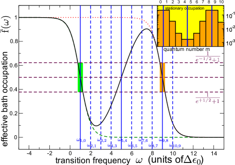
Figure 1: (Color Online) Effective bath occupation (solid black) in Eq. (28) generated by two fermionic baths (dotted red and dashed green curves, chemical potentials $\mu^{(k)}$ and temperatures $\left[\beta^{(k)}\right]^{-1}$ are given by the center and width of the shaded boxes, respectively) with Lorentzian tunneling rates of form (29). The detuning of the tunneling rates is adjusted such that the average hypothetical occupation function $\bar{\rm f}(\omega)$ is not monotonically decaying. Then, the threshold $1/2$ is passed several times (vertical solid blue lines) within the transition frequency window probed by the system. This will lead to an increasing population $\rho_{m+1}>\rho_{m}$ when $\bar{\rm f}(\omega_{m+1,m})>1/2$ and to a decreasing population $\rho_{m+1}<\rho_{m}$ when $\bar{\rm f}(\omega_{m+1,m})<1/2$ (compare the inset). Such multi-modal distributions are clearly non-thermal, i.e., they cannot be generated by a single thermal bath by adjusting temperature and chemical potential. Parameters have been chosen as $\Delta\epsilon_{0}\beta^{(1)}=\Delta\epsilon_{0}\beta^{(2)}=2$, $\mu^{(1)}=\Delta\epsilon_{0}$, $\mu^{(2)}=9\Delta\epsilon_{0}$, $\Gamma_{1}=\Gamma_{2}$, $\delta_{1}=\delta_{2}=0.1\Delta\epsilon_{0}$, and $\bar{\omega}_{1}=\Delta\epsilon_{0}$ with $\bar{\omega}_{2}=9\Delta\epsilon_{0}$. The shown equidistant transition frequencies (vertical solid and dashed blue lines) correspond to eigenvalues that scale quadratically with $m$ and may be realized by the example in Sec. IV.1 by using $N=10$, $\epsilon=\Delta\epsilon_{0}$, $U=\Delta\epsilon_{0}$, and $T=0$.

When the average occupation function at the transition frequency $\omega_{m+1,m}$ between states $\left|m\right>$ and $\left|m+1\right>$ exceeds 1/2, the population of the states will increase $\rho_{m+1}>\rho_{m}$, whereas the opposite is true for $\bar{{\rm f}}(\omega_{m+1,m})<1/2$, see Fig. 1. Depending on the number and the thermal properties used baths, the resulting hypothetical average distribution (28) may assume quite arbitrary shapes, such that more sophisticated statistical stationary mixtures than in Fig. 1 are conceivable.

III.4 Trivial dynamic equilibria

It has been observed for special systems segal2008a that the equilibrium state had a thermal form with some average temperature even though the system of interest was coupled to more than just a single thermal bath with different temperatures. For the ladder-like systems discussed in the previous section, it is obvious that to describe the stationary state with just two parameters $\bar{\beta}$ and $\bar{\mu}$ requires Eqns. (27) to be compatible with

$$\frac{\bar{\rho}_{m+1}}{\bar{\rho}_{m}} = \frac{\bar{F}_{\pm}(\omega_{m+1,m})}{1\pm\bar{F}_{\pm}(\omega_{m+1,m})}\stackrel{{\scriptstyle!}}{{=}}e^{-\bar{\beta}(\omega_{m+1,m}-\bar{\mu})}\,,$$ (30)

where the effective average occupation is defined in Eq. (28). This can be achieved in several possible ways:

Firstly, for a three-dimensional system Hilbert space ($N=2$ in the previous section), we will only have two transition frequencies and accordingly only two equations of the above form. These two equations would uniquely fix the parameters $\bar{\beta}$ and $\bar{\mu}$. Note however, that then in general $\bar{\beta}<0$ is possible, which corresponds to population inversion (i.e., favoring for $\bar{\mu}=0$ the most excited state) Evidently, this forbids the interpretation of the parameter $\bar{\beta}$ as inverse temperature.

Alternatively, for $N>2$, Eqns. (27) may still be linearly dependent, as is the case when the system Hamiltonian provides only a single transition frequency (e.g., a harmonic oscillator). In an approximate sense, linear dependence may also be generated when the average occupation function $\bar{F}_{\pm}(\omega)$ is essentially flat in the transition frequency window probed by the system. Assuming only a single transition frequency $\Omega$, such that the tunneling rates are described by a single number $G^{(k)}(\Omega)\equiv\Gamma_{k}$, and vanishing chemical potentials $\mu^{(k)}=0=\bar{\mu}$ in the low-energy limit $\beta^{(k)}\Omega\ll 1$, Eqn. (27) defines average temperatures for bosons and fermions

$$\bar{T}_{\rm Bose} \approx \sum_{k}\frac{\Gamma_{k}}{\Gamma}T^{(k)}\,,$$

$$\frac{1}{\bar{T}_{\rm Fermi}} \approx \sum_{k}\frac{\Gamma_{k}}{\Gamma}\frac{1}{T^{(k)}}$$ (31)

with $\Gamma\equiv\sum_{\ell}\Gamma_{\ell}$, that correspond to the weighted arithmetic (bosons) and weighted harmonic (fermions) mean. The bosonic average temperature does well resemble the Richmann mixing formula and has been found previously segal2008a . However, it should be noted that this is different from the so-called classical (high-energy) limit $\beta^{(k)}\Omega\gg 1$, for which one obtains an arithmetic mean of the Boltzmann factors from Eq. (27)

$$e^{-\bar{\beta}\Omega}\approx\sum_{k}\frac{\Gamma_{k}}{\Gamma}e^{-\beta^{(k)}\Omega}$$ (32)

for – as expected – both fermionic and bosonic baths.

IV Examples

For a single reservoir the equilibration of both temperature and chemical potential has been observed for interacting double dots schaller2009b in the BMS approximation. Therefore, we only give examples to illustrate the results in Sec. III.2, Sec. III.3, and Sec. III.4. Naturally, in case of only a single coupling bath, the case of Sec. III.1 is also reproduced here.

IV.1 Homogeneous Electronic Nanostructure

Consider a nanostructure with $N$ homogenous electronic sites (we neglect the spin)

$$H_{\rm S}=\epsilon\sum_{i=1}^{N}d_{i}^{\dagger}d_{i}+\frac{U}{2}\sum_{i\neq j}d_{i}^{\dagger}d_{i}d_{j}^{\dagger}d_{j}+T\sum_{i\neq j}d_{i}^{\dagger}d_{j}$$ (33)

with single-particle energy $\epsilon$, Coulomb interaction $U$, and hopping term $T$ that are all assumed completely isotropic. The permutational symmetry suggests to reduce the problem to the symmetrized subspace with the basis $\left|N,m+1\right>\equiv\frac{1}{\sqrt{(N-m)(m+1)}}D^{\dagger}\left|N,m\right>$ with $0\leq m\leq N$ denoting the number of electrons in the system, where $D\equiv\sum_{i=1}^{N}d_{i}$ and $\left|N,0\right>=\left|0,\ldots,0\right>$ represents the $N$ particle Fock space vacuum. Clearly, both $H_{\rm S}$ and $N_{S}\equiv\sum_{i}d_{i}^{\dagger}d_{i}$ are diagonal in this basis. For $N=1$ we recover the single resonant level haug2008 , but for for $N>1$, the spectrum of the system Hamiltonian becomes nontrivial. The eigenvalues of the symmetric subspace read $E_{m}=m\epsilon+m(m-1)U/2+m(N-m)T$, such that the spectrum may become equidistant when $U=2T$ with $\omega_{m+1,m}\to\epsilon+(N-1)T$ – which still admits a strongly interacting model.

At first we assume that the nanostructure is only coupled to a single lead $H_{\rm B}=\sum_{k}\epsilon_{k}c_{k}^{\dagger}c_{k}$ at temperature $\beta$ and chemical potential $\mu$ via the tunneling Hamiltonian  $H_{\rm SB}=D\otimes\sum_{k}g_{k}c_{k}^{\dagger}+D^{\dagger}\otimes\sum_{k}g_{k}^{*}c_{k}$, where $g_{k}$ represents a frequency-dependent coupling constant, and $c_{k}$ are fermionic annihilation operators acting on the lead Hilbert space. The conserved quantity is composed from $N_{S}$ and $N_{B}=\sum_{k}c_{k}^{\dagger}c_{k}$. We may write the interaction Hamiltonian also as $H_{\rm SB}=A_{1}\otimes B_{1}+A_{2}\otimes B_{2}$, with the hermitian and trace-orthogonal (not-normalized) system coupling operators $A_{1}=\left(D^{\dagger}+D\right)$ and $A_{2}=i\left(D^{\dagger}-D\right)$, and the associated hermitian bath coupling operators $B_{1}=\sum_{k}\left(g_{k}c_{k}^{\dagger}+g_{k}^{*}c_{k}\right)/2$ and $B_{2}=i\sum_{k}\left(g_{k}c_{k}^{\dagger}-g_{k}^{*}c_{k}\right)/2$. For a bath in thermal equilibrium with inverse temperature $\beta$ and chemical potential $\mu$, such that its density matrix is given by Eq. (11), we obtain for Fourier transforms (I) of the bath correlation functions $\gamma_{11}(\omega)=\gamma_{22}(\omega)=\Gamma(+\omega)\left[1-{\rm f}(+\omega)\right]/4+\Gamma(-\omega){\rm f}(-\omega)/4$ and $\gamma_{12}(\omega)=\gamma_{21}^{*}(\omega)=i\Gamma(+\omega)\left[1-{\rm f}(+\omega)\right]/4-i\Gamma(-\omega){\rm f}(-\omega)/4$, where $\Gamma(\omega)\equiv 2\pi\sum_{k}{\left|g_{k}\right|}^{2}\delta(\omega-\epsilon_{k})$ is the tunneling rate and the Fermi function ${\rm f}(\omega)$ encodes the bath properties $\beta$ and $\mu$, compare Eq. (25). Obviously, the Fourier-transform matrix of bath correlation functions has non-negative eigenvalues – a consequence of Bochners theorem breuer2002 ; reed1975 . These lead to the non-vanishing dampening coefficients

$$\tilde{\gamma}_{m,m+1} = (N-m)(m+1)\Gamma(\omega_{m+1,m})\left[1-{\rm f}(\omega_{m+1,m})\right]\,,$$

$$\tilde{\gamma}_{m+1,m} = (N-m)(m+1)\Gamma(\omega_{m+1,m}){\rm f}(\omega_{m+1,m})\,,$$ (34)

where $\omega_{m+1,m}\equiv E_{m+1}-E_{m}$ and the factoring condition (III.3) is obviously fulfilled. We obtain a rate equation of the form (22) with $\rho_{m}\equiv\left<N,m\right|\rho_{\rm S}\left|N,m\right>$, where the Lamb-shift terms are irrelevant, since we have by exploiting the permutational symmetry mapped our system to a nondegenerate one.

Now we consider tunnel couplings to multiple baths with factorizing density matrices as in Eq. (20). The form of Eq. (22) remains invariant, and we simply have $\tilde{\gamma}_{m,m\pm 1}=\sum_{k}\tilde{\gamma}_{m,m\pm 1}^{(k)}$, with different temperatures $\beta^{(k)}$ and chemical potentials $\mu^{(k)}$ entering the rates as in Eq. (IV.1). The general non-equilibrium steady state of Eq. (22) fulfills

$$\frac{\bar{\rho}_{m+1}}{\bar{\rho}_{m}}=\frac{\sum_{k}\Gamma^{(k)}(\omega_{m+1,m}){\rm f}^{(k)}(\omega_{m+1,m})}{\sum_{k}\Gamma^{(k)}(\omega_{m+1,m})\left[1-{\rm f}^{(k)}(\omega_{m+1,m})\right]}$$ (35)

and is thus identical with the non-equilibrium steady state for coupling to a single hypothetical non-equilibrium bath with average non-thermal distribution of the form (28), compare also Fig. 1.

IV.2 Coupled oscillators

We consider a harmonic oscillator $H_{\rm S}=\Omega b^{\dagger}b$ coupled to many others $H_{\rm B}=\sum_{k}\omega_{k}b_{k}^{\dagger}b_{k}$ with positive eigenfrequencies $\omega_{k}>0$ via quasi-particle tunneling $H_{\rm SB}=b\otimes\sum_{k}h_{k}b_{k}^{\dagger}+b^{\dagger}\otimes\sum_{k}h_{k}^{*}b_{k}$. The conserved quantity is composed from $N_{S}=b^{\dagger}b$ and $N_{B}=\sum_{k}b_{k}^{\dagger}b_{k}$. Rewriting the interaction Hamiltonian in terms of hermitian operators, we obtain $A_{1}=(b^{\dagger}+b)$, $A_{2}=i(b^{\dagger}-b)$, $B_{1}=\sum_{k}(h_{k}b_{k}^{\dagger}+h_{k}^{*}b_{k})/2$, and $B_{2}=i\sum_{k}(h_{k}b_{k}^{\dagger}-h_{k}^{*}b_{k})/2$. The matrix elements of the Fourier transforms (I) of the bath correlation functions equate to $\gamma_{11}(\omega)=\gamma_{22}(\omega)=1/4\left[+\Theta(+\omega)[1+\rm n(+\omega)]\Gamma(+\omega)+\Theta(-\omega)\rm n(-\omega)\Gamma(-\omega)\right]$ for the diagonals and $\gamma_{21}^{*}(\omega)=\gamma_{12}(\omega)=i/4\left[+\Theta(+\omega)[1+\rm n(+\omega)]\Gamma(+\omega)-\Theta(-\omega)\rm n(-\omega)\Gamma(-\omega)\right]$ for the off-diagonals, where $\Theta(\omega)$ denotes the Heaviside step function, $\Gamma(\omega)\equiv 2\pi\sum_{k}{\left|h_{k}\right|}^{2}\delta(\omega-\omega_{k})$ the quasi-particle tunneling rate, and $\rm n(\omega)$ denotes the bosonic occupation number as defined in Eq. (26). The condition that $\mu<\min_{k}(\omega_{k})$ grants positivity of all bath occupations. In addition, it implies that $\left.\Gamma(\Omega)\right|_{\Omega<\mu}=0$, such that we assume also $\Omega>\mu$ throughout. Accordingly, the Fourier transform matrix of the bath correlation functions is positive semidefinite at all frequencies. In the Fock space basis (where $b^{\dagger}\left|n\right>=\sqrt{n+1}\left|n+1\right>$), we obtain a rate equation of the form (22), where $0\leq n<\infty$. However, since even the original eigenstates are non-degenerate, the dampening coefficients equate (with $\Omega>0$) to

$$\tilde{\gamma}_{n,n+1} = (n+1)\Gamma(\Omega)\left[1+\rm n(\Omega)\right]\,,$$

$$\tilde{\gamma}_{n+1,n} = (n+1)\Gamma(\Omega)\rm n(\Omega)\,,$$ (36)

which is also compatible with assumption (III.3). The resulting system is infinitely large, one may however, introduce a cutoff size $N_{\rm cut}$ and solve for the stationary state of the rate equations for finite $N_{\rm cut}$. The ratio $\rho_{n+1}/\rho_{n}$ of two successive populations yields the desired Boltzmann factor, which even happens to be independent of $N_{\rm cut}$.

For multiple baths, we obtain equilibration in a thermal state with the unique generalized Boltzmann factor

$$\frac{\rho_{n+1}}{\rho_{n}}=\frac{\sum_{k}\Gamma^{(k)}(\Omega)\rm n^{(k)}(\Omega)}{\sum_{k}\Gamma^{(k)}(\Omega)\left[1+\rm n^{(k)}(\Omega)\right]}\,,$$ (37)

consistent with Eq. (27). This generalized Boltzmann factor is the same that one would obtain for contact with a single hypothetical non-thermal bath at an average occupation compatible with Eq. (28), which in the high-temperature and $\mu^{(k)}\to 0$ limit reduces to the bosonic average temperature in Eq. (III.4). This coincides well with the well-known temperature mixing formula and previous results segal2008a .

IV.3 Spin-Boson Model

A variant of the spin-boson model coupled to a single bath has already been provided in Ref. vogl2010a , such that we here only generalize to $K\geq 2$ baths and non-vanishing chemical potentials. We consider a large spin system $H_{\rm S}=\Omega/2J^{z}$ with $\Omega>0$, coupled to a bath of harmonic oscillators $H_{\rm B}=\sum_{k}\omega_{k}b_{k}^{\dagger}b_{k}$ with $\omega_{k}>0$ via $H_{\rm SB}=J^{+}\otimes\sum_{k}h_{k}b_{k}^{\dagger}+J^{-}\otimes\sum_{k}h_{k}b_{k}$, where $J^{\alpha}\equiv\sum_{i=1}^{N}\sigma^{\alpha}_{i}$ and $\sigma^{\pm}=(\sigma^{x}\pm i\sigma^{y})/2$. The conserved quantity is given by $N_{S}+N_{B}=-J^{z}/2+\sum_{k}b_{k}^{\dagger}b_{k}$. We impose the same conditions on the chemical potential(s) as before: $\mu<\min_{k}(\omega_{k})$ and $\mu<\Omega$. Choosing the system coupling operators as $A_{1}=J^{x}$ and $A_{2}=J^{y}$, the Fourier transforms (I) of the bath correlation function are identical to the previous section. In order to calculate the dampening coefficients, permutational symmetry suggests to use the angular momentum basis $\left|N/2,m\right>$ with $-N/2\leq m\leq+N/2$. Using that $J^{\pm}\left|j,m\right>=\sqrt{j(j+1)-m(m\pm 1)}\left|j,m\pm 1\right>$, we obtain a rate equation of the form (22) with the coefficients

$$\tilde{\gamma}_{m,m+1} = \left[\frac{N}{2}\left(\frac{N}{2}+1\right)-m(m+1)\right]\Gamma(\Omega)\left[1+\rm n(\Omega)\right]\,,$$

$$\tilde{\gamma}_{m+1,m} = \left[\frac{N}{2}\left(\frac{N}{2}+1\right)-m(m+1)\right]\Gamma(\Omega)\rm n(\Omega)\,.$$ (38)

Solving this rate equation with multiple baths for its steady state yields a thermal bath with the same unique generalized Boltzmann factor as Eq. (37), as predicted by Eq. (27).

IV.4 Mixed Spin Model

We consider a spin-1/2 system $H_{\rm S}=\Omega/2\sigma^{z}$ that is firstly coupled to a bosonic bath $H_{\rm B}^{(1)}=\sum_{k}\omega_{k}b_{k}^{\dagger}b_{k}$ via the dissipative coupling $H_{\rm SB}^{(1)}=\sigma^{+}\otimes\sum_{k}h_{k}b_{k}^{\dagger}+\sigma^{-}\otimes\sum_{k}h_{k}^{*}b_{k}$, and secondly to a fermionic bath $H_{\rm B}^{(2)}=\sum_{k}\epsilon_{k}c_{k}^{\dagger}c_{k}$ via the coupling $H_{\rm SB}^{(2)}=\sigma^{+}\otimes\sum_{k}g_{k}c_{k}^{\dagger}+\sigma^{-}\otimes\sum_{k}g_{k}^{*}c_{k}$. Note that in contrast to the previous examples we do now consider two different baths from the beginning. The interaction Hamiltonians explicitly obeys the conserved quantity constructed from $N_{S}=-\sigma^{z}/2$, $N_{B}^{(1)}=\sum_{k}b_{k}^{\dagger}b_{k}$, and $N_{B}^{(2)}=\sum_{k}c_{k}^{\dagger}c_{k}$. Note that $H_{\rm SB}^{(2)}$ does not conserve the number of fermions, but such a model may represent scattering processes with a further fermionic bath that omitted from the description. As before, we require that $\mu^{(1)}<\Omega$ and $\mu^{(1)}<\min_{k}(\omega_{k})$. Choosing the system coupling operators as $A_{1}=\sigma^{x}$ and $A_{2}=\sigma^{y}$, we obtain $B_{1}^{(1)}=1/2\sum_{k}\left(h_{k}b_{k}^{\dagger}+h_{k}^{*}b_{k}\right)$, $B_{2}^{(1)}=i/2\sum_{k}\left(h_{k}b_{k}^{\dagger}-h_{k}^{*}b_{k}\right)$, and $B_{1}^{(2)}=1/2\sum_{k}\left(g_{k}c_{k}^{\dagger}+g_{k}^{*}c_{k}\right)$ with $B_{2}^{(2)}=i/2\sum_{k}\left(g_{k}c_{k}^{\dagger}-g_{k}^{*}c_{k}\right)$. The Fourier transform of the bath correlation function for the first bath corresponds to Sec. IV.3, whereas the Fourier transform matrix for the second bath is identical to that of Sec. IV.1. Accordingly, we obtain in the $\sigma^{z}$-eigenbasis $\sigma^{z}\left|a\right>=(-1)^{a}\left|a\right>$ with $a\in\{0,1\}$ and $\rho_{a}\equiv\left<a\right|\rho_{\rm S}\left|a\right>$ the master equation

$$\rho_{0} = -\left[\tilde{\gamma}_{1,0}^{(1)}+\gamma_{1,0}^{(2)}\right]\rho_{0}+\left[\tilde{\gamma}_{0,1}^{(1)}+\gamma_{0,1}^{(2)}\right]\rho_{1}\,,$$

$$\rho_{1} = +\left[\tilde{\gamma}_{1,0}^{(1)}+\gamma_{1,0}^{(2)}\right]\rho_{0}-\left[\tilde{\gamma}_{0,1}^{(1)}+\gamma_{0,1}^{(2)}\right]\rho_{1}$$ (39)

with the dampening coefficients $\tilde{\gamma}_{0,1}^{(1)}=\Gamma_{1}(\Omega)\left[1+\rm n(\Omega)\right]$, $\tilde{\gamma}_{1,0}^{(1)}=\Gamma_{1}(\Omega)\rm n(\Omega)$, $\tilde{\gamma}_{0,1}^{(2)}=\Gamma_{2}(\Omega)\left[1-{\rm f}(\Omega)\right]$, and $\tilde{\gamma}_{1,0}^{(2)}=\Gamma_{2}(\Omega){\rm f}(\Omega)$, where ${\rm f}(\omega)$ and $\rm n(\omega)$ have been defined in Eqns. (25) and (26), respectively, and $\Gamma_{1}(\omega)=2\pi\sum_{k}{\left|h_{k}\right|}^{2}\delta(\omega-\omega_{k})$ with $\Gamma_{2}(\omega)=2\pi\sum_{k}{\left|g_{k}\right|}^{2}\delta(\omega-\epsilon_{k})$ represent the coupling strengths to the two baths, respectively. The stationary state of Eq. (IV.4) is characterized by the generalized Boltzmann factor

$$\frac{\rho_{1}}{\rho_{0}}=\frac{\Gamma_{1}(\Omega)\rm n(\Omega)+\Gamma_{2}(\Omega){\rm f}(\Omega)}{\Gamma_{1}(\Omega)\left[1+\rm n(\Omega)\right]+\Gamma_{2}(\Omega)\left[1-{\rm f}(\Omega)\right]}\,,$$ (40)

which is consistent with Eq. (27).

V Conclusions

Under the Born, Markov, and secular approximations, quantum systems coupled to a single bath described by inverse temperature $\beta$ and chemical potential $\mu$ relax – when the total Hamiltonian conserves a (quasi-)particle number – into a stationary equilibrium ensemble that is described by the same inverse temperature and the same chemical potential. As long as only a single bath is involved, this also holds when the spectrum of the system Hamiltonian is not equidistant.

For coupling to multiple thermal baths and tridiagonal rate equations, a hypothetical non-thermal average bath is effectively felt by the system, which will in general lead to a non-thermal stationary state. However, when there exists only a single transition frequency as e.g. in two-level systems, the resulting stationary state may be well characterized by a single Boltzmann factor with two parameters $\bar{\beta}$ and $\bar{\mu}$. The possibility of creating level inversion however demonstrates that then $\bar{\beta}$ does not always define an inverse temperature.

There are several interesting consequences: Firstly, by using equilibration under side constraints one should be able to prepare not only the ground state of a system Hamiltonian by dissipative means but also an energetically sufficiently isolated energy eigenstate with a desired particle number when temperature and chemical potential of a single grand-canonical bath are tuned accordingly. Secondly, in order to generate interesting non-equilibrium stationary states via coupling to multiple baths, fermionic baths appear more favorable. Beyond this, it is necessary (though not sufficient) to consider system Hamiltonians with multiple allowed transition frequencies. Energy-dependent tunneling rates can then significantly enhance the non-thermal signatures of the resulting stationary state. Finally, when the focus is on particle or thermal transport, the quantities of interest are often the stationary current through the system and its fluctuations (noise), see e.g. Refs. braun2006a ; aghassi2006a . The calculation of these quantities heavily depends on the knowledge of the stationary state and may therefore strongly benefit from its analytic knowledge.

VI Acknowledgments

Financial support by the DFG (Project SCHA 1646/2-1) is gratefully acknowledged. The author has benefited from discussions with T. Brandes, M. Esposito, G. Kießlich, and M. Vogl.

References

- (1) M. Srednicki, Phys. Rev. E 50, 888 (1994).
- (2) N. Linden, S. Popescu, A. J. Short, and A. Winter, Phys. Rev. E 79, 061103 (2009).
- (3) H.-P. Breuer and F. Petruccione, The Theory of Open Quantum Systems, (Oxford University Press, Oxford, 2002).
- (4) M. Schlosshauer, Decoherence and the quantum-to-classical transition, (Springer, Berlin, 2008)
- (5) G. Lindblad, Commun. Math. Phys. 48, 119, (1976).
- (6) V. Gorini, A. Frigerio, M. Verri, A. Kossakowski, and E. C. G. Sudarshan, Rep. Math. Phys. 13, 149 (1978).
- (7) H. Wichterich, M. J. Henrich, H.-P. Breuer, J. Gemmer, and M. Michel, Phys. Rev. E 76, 031115 (2007).
- (8) D. A. Lidar, Z. Bihary, and K. B. Whaley, Chem. Phys. 268, 35 (2001).
- (9) A. Kossakowski, A. Frigerio, V. Gorini, and M. Verri, Comm. Math. Phys. 57, 97 (1977).
- (10) D. Segal, Phys. Rev. E 77, 021103 (2008).
- (11) T. H. Stoof and Yu. V. Nazarov, Phys. Rev. B 53, 1050 (1996).
- (12) S. A. Gurvitz and Ya. S. Prager, Phys. Rev. B 53, 15932 (1996).
- (13) H. Förster and M. Büttiker, Phys. Rev. Lett. 101, 136805 (2008).
- (14) G. Schaller and T. Brandes, Phys. Rev. A 78, 022106 (2008).
- (15) M. Braun and J. König and J. Martinek, Phys. Rev. B 70, 195345 (2004).
- (16) G. Schaller and P. Zedler and T. Brandes, Phys. Rev. A 79, 032110 (2009).
- (17) R. Kubo, J. Phys. Soc. Jap. 12, 570 (1957).
- (18) P. C. Martin and J. Schwinger, Phys. Rev. 115, 1342 (1959).
- (19) R. Kubo, Rep. Prog. Phys. 29, 255 (1966).
- (20) M. Esposito, U. Harbola, and S. Mukamel, Rev. Mod. Phys. 81, 1665 (2009).
- (21) G. Schaller, G. Kießlich and T. Brandes, Phys. Rev. B 80, 245107 (2009).
- (22) M. Znidaric, T. Prosen, G. Benenti, G. Casati, and D. Rossini, Phys. Rev. E 81, 051135 (2010).
- (23) M. Rigol, V. Dunjko, and M. Olshanii, Nature 452, 854 (2008).
- (24) M. Esposito, U. Harbola, and S. Mukamel, Phys. Rev. E 76, 031132 (2007).
- (25) K. Saito and Y. Utsumi, Phys. Rev. B 78, 115429 (2008).
- (26) B. Elattari and S. A. Gurvitz, Phys. Rev. A 62, 032102 (2000).
- (27) P. Zedler and G. Schaller and G. Kießlich and C. Emary and T. Brandes, Phys. Rev. B 80, 045309 (2009).
- (28) H. Haug and A.-P. Jauho, Quantum Kinetics in Transport and Optics of Semiconductors, (Springer, Berlin, 2008).
- (29) M. Reed and B. Simon, Methods of Modern Mathematical Physics, vol. II, (Academic Press, London, 1975).
- (30) M. Vogl, G. Schaller, and T. Brandes, Phys. Rev. A 81, 012102 (2010).
- (31) M. Braun, J. König, and J. Martinek, Phys. Rev. B 74, 075328 (2006).
- (32) J. Aghassi, A. Thielmann, M. H. Hettler, G. Schön, Phys. Rev. B 73, 195323 (2006).