Localization in momentum space of ultracold atoms in incommensurate lattices

Abstract

We characterize the disorder induced localization in momentum space for ultracold atoms in one-dimensional incommensurate lattices, according to the dual Aubry-André model. For low disorder the system is localized in momentum space, and the momentum distribution exhibits time-periodic oscillations of the relative intensity of its components. The behavior of these oscillations is explained by means of a simple three-mode approximation. We predict their frequency and visibility by using typical parameters of feasible experiments. Above the transition the system diffuses in momentum space, and the oscillations vanish when averaged over different realizations, offering a clear signature of the transition.

I Introduction

Disorder is among the most intriguing and ubiquitous aspects of condensed matter kramer . The prediction of localization induced by a random disorder in a periodic lattice dates back to the seminal work by Anderson anderson1958 . Recently, ultracold atomic gases have demonstrated to be an extremely versatile tool to explore the effects of disorder, owing to the great tunability of the system parameters and geometrical configurations fallani2008 ; billy2008 ; roati2008 ; deissler2010 ; demarco . Notably, Anderson localization of matter waves has been observed both for correlated (speckle) disorder billy2008 and quasi-periodic optical lattices roati2008 , the latter case realizing the so-called Aubry-André (AA) model harper1955 ; aubry1980 . Localization effects in the quantum dynamics of one-dimensional lattice models have attracted a large interest also in the recent theoretical literature larcher2009 ; interaction_vs_localization ; others . The AA model has the peculiar property of exhibiting a transition, already in one dimension and both in real and momentum space (duality), from extended to exponentially localized states as the disorder strength is increased above a critical value aubry1980 ; aulbach2004 ; lahini2009 . So far the evolution of wave packets in the AA model has been investigated mainly in real space, looking for signatures of the transition from ballistic spreading to sub-diffusion and localization, both in theory hiramoto1988 ; larcher2009 and experiments roati2008 ; lahini2009 .

Here we focus on the dynamics of the momentum distribution and identify measurable effects of the transition from diffusion to localization in momentum space. This is relevant for current experiments with ultracold atoms, where the momentum distribution is accessible via time of flight measurements and, typically, with an higher accuracy than in real space. In addition, it provides complementary information for a better understanding of the key role played by duality of the AA model.

II Aubry-Andrè model

The quantum dynamics of the AA model for the amplitude $\psi_{n}(t)$ is governed by the equation

$$i\partial_{t}\psi_{n}=-[\psi_{n+1}+\psi_{n-1}]+\lambda\cos(2\pi\alpha n+\varphi)\psi_{n}$$ (1)

where $\lambda$ is the disorder strength, and $\varphi$ an arbitrary phase. This equation can be used to model non-interacting atoms subject to two periodic optical lattices with different wavelengths, that is, a bichromatic lattice roati2008 ; deissler2010 . In this case, $\alpha$ is the ratio between their wavelengths. In the tight-binding regime, Eq. (1) is easily obtained starting from the Schrödinger equation and projecting the continuous wave function $\psi(x)$ on the basis of the Wannier functions, $w_{n}(x)$, of the lowest band of the primary lattice modugno2009 , $\psi(x)=\sum_{n}\psi_{n}w_{n}(x)$, where $n$ is the lattice site index. The secondary lattice appears in the last term of Eq. (1) in the form of a modulation which mimics a disorder (quasi-disorder). Without any loss of generality, one can choose $\alpha<1$, because Eq. (1) is invariant under a shift of $\alpha$ by an integer number. When $\alpha$ is a rational number one can write it as $\alpha=p/q$ and the solution of Eq. (1) can be restricted to a region of size $N=q$, which coincides with spatial periodicity of the system. The case of irrational $\alpha$ can be obtained as a limit of a continued fraction approximation.

Aubry-André showed aubry1980 that this model has a duality under the following transformation

$${\phi_{l}}=N^{-1/2}\sum_{n}\psi_{n}e^{in[{2\pi}\alpha l+\theta]}e^{-i\varphi l}$$ (2)

which maps Eq. (1) into an equation for the new variable $\phi_{l}$ exactly of the same form as Eq. (1) but with disorder strength $4/\lambda$. This transformation corresponds to a projection on a basis of quasi-momentum eigestates with eigenvalues $\xi=2\pi\alpha l+\theta=(2\pi/N)pl+\theta$, where $\xi$ is defined in the first Brillouin zone, $\xi\in[-\pi,\pi]$. By using this duality one can show that the AA model undergoes a transition from an extended to a localized regime at $\lambda=2$.

In the AA model the space is discrete and one can conveniently introduce the discrete Fourier transform (DFT)

$$f_{k}=N^{-1/2}\sum_{n}\psi_{n}e^{-i\frac{2\pi}{N}kn}$$ (3)

which corresponds to a projection on the basis of quasi-momentum eigenstates with eigenvalues $\xi=(2\pi/N)k$. The relation bewteen momentum and quasi-momentum distributions is $|\tilde{\psi}(k,t)|^{2}={N}|f_{k}(t)|^{2}|\tilde{w}(k)|^{2}$ where $\tilde{w}(k)$ is the Fourier transform of the Wannier function centered on the lattice site $n=0$. Note also that the expression (3) is related to the dual mapping (2) by an arbitrary shift of $\theta$ and a permutation aulbach2004 . By applying the transformation (3) to the AA model one gets modugno2009

$$i\partial_{t}f_{k}=-2\cos\left(\frac{2\pi k}{N}\right)f_{k}+\frac{\lambda}{2}\left[e^{-i\varphi}f_{k+p}+e^{i\varphi}f_{k-p}\right]$$ (4)

which is the equation describing the evolution in momentum space. Owing to the duality of the AA model under the transformation (2), and to the similarity of the latter with Eq. (3), the localization properties in momentum space are the same of the dual AA model, except for the fact that disorder couples modes differing by $|\Delta\xi|=2\pi\alpha$ instead of neighboring ones.

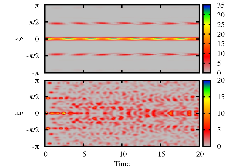
Figure 1: (Color online) Quasi-momentum distribution $|f_{k}(t)|^{2}$ obtained from the DFT of the solution of Eq (1). The index $\xi$ is related to $k$ by $\xi=2\pi k/N$. Here we use $\alpha=0.2282...$ and $\varphi=0$. The initial wave packet in real space is a Gaussian of width $\sigma=10$. Time is given in dimensionless units. Top panel: $\lambda=1$, only few modes are involved and a periodic oscillation of the central and side peaks is observed. The side peaks are at a distance $\pm 2\pi\alpha$ from the central peak. Bottom panel: $\lambda=5$, the evolution is affected by the coupling of many modes and the periodic oscillations are no more visible.

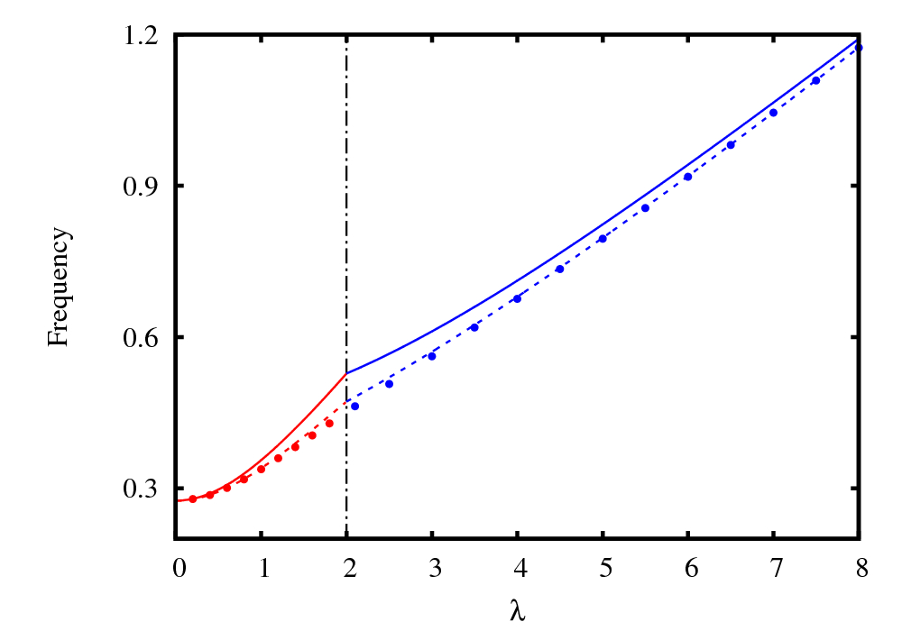
Figure 2: (Color online) Oscillation frequency of the central peak of quasi-momentum ($\lambda<2$, red) and spatial ($\lambda>2$, blue) distributions, for $\sigma=10$, $\varphi=0$. The full solution of the AA model (dots) is compared with the predictions of an analytic three-mode approximation (full lines) and a semi-analytic five-mode approximation (dashed line).

III Results and discussions

In the following we will consider the evolution of a wave packet, by solving Eq. (1) in real space and then computing the evolution in momentum space by means of the DFT numerics . As initial condition we choose a Gaussian wave packet, $\psi_{j}(0)=A\exp\{-{j^{2}}/{2\sigma^{2}}\}$, where $\sigma$ is the width and $A$ is a normalization factor. This choice is convenient if one wants to simulate realistic experimental configurations; it also allows one to explore the behavior of sharp to broad wave packets in a continuous manner.

According to the previous discussion, localization in momentum space occurs for $\lambda<2$, where the wave packet instead spreads in real space. In this regime one thus expects to see only one or few momentum components significantly populated. Conversely, for $\lambda>2$ the regime is diffusive in momentum space and localized in real space, and one should see a momentum distribution with many modes coupled together during the evolution of the system. This is indeed confirmed by our numerical simulations, as shown in Fig. 1 (the value $\alpha=1064.4/866.6-1=0.2282...$ has been chosen in order to model the bichromatic lattice of the experiment of Ref. deissler2010 ). A striking feature is that, for $\lambda<2$, the quasi-momentum components $|f_{k}|^{2}$ exhibit periodic oscillations, occurring among the central peak and two side peaks at distance $\pm 2\pi\alpha$. The numerical result for the frequency of these oscillations is plotted in Fig. 2 as a function of $\lambda$ (red points for $\lambda<2$) (frequency, ).

This oscillating behavior can be understood in terms of the following model. Let us assume that the width $1/\sigma$ of the initial quasi-momentum distribution is small enough, so that only the $k=0$ mode can be considered populated at $t=0$ ($f_{k}(0)=\delta_{k,0}$) and the time evolution couples the mode at $k=0$ with two side modes at $k=\pm p$ only (i.e., $\xi=0$ and $\pm 2\pi\alpha$, respectively). This assumption is valid when $1/{\sigma}\lesssim 2\pi\alpha$. In this way, the AA equation is mapped into an eigenvalue problem of a $3\times 3$ matrix, whose eigenvectors and eigenvalues can be written as $g_{k,j}$ and $E_{j}$, respectively, with $j=1,2,3$. The initial condition is $f_{k}(0)=\sum_{j=1}^{3}\gamma_{j}g_{k,j}$, where the coefficients $\gamma_{j}$ are given by the standard rules of quantum mechanics. Under these assumptions one has $\gamma_{j=3}\equiv 0$, and the time evolution takes the form

$$|f_{k}(t)|^{2}= (\gamma_{1}g_{k,1})^{2}+(\gamma_{2}g_{k,2})^{2}$$

$$+\gamma_{1}\gamma_{2}g_{k,1}g_{k,2}\cos\left[(E_{2}-E_{1})t\right]\,.$$ (5)

This expression describes a time-periodic oscillation of the relative intensity of the central and side peaks, with frequency $\nu(\lambda<2)=|E_{2}-E_{1}|/2\pi$, given by

$$\nu(\lambda<2)=\pi^{-1}\sqrt{[1-\cos(2\pi\alpha)]^{2}+\lambda^{2}/2}\,.$$ (6)

It is worth stressing that, once $\alpha$ is fixed, this frequency depends only on the disorder strength $\lambda$, but not on the phase $\varphi$. This three-mode approximation provides a reasonable description of the numerical results, as shown by the solid line for $\lambda<2$ in Fig. 2.

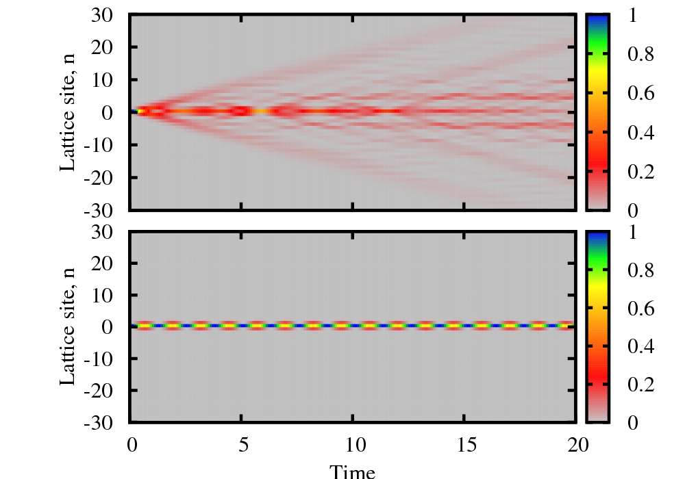
Figure 3: (Color online) Spatial distribution $|\psi_{n}|^{2}$ obtained from the solution of Eq (1) using a single site initial condition $\psi_{n}=\delta_{n,0}$. As in Fig. 1, we use $\alpha=0.2282...$ and $\varphi=0$. Time is given in dimensionless units. Top panel: $\lambda=1$, the initially localized wavepacket spreads ballistically and there are no visible periodic oscillations. Bottom panel: $\lambda=5$, the wave packet is localized and a periodic oscillation of the central peak and its nearest neighbors is clearly visible.

The three-mode approximation becomes inaccurate when approaching $\lambda=2$, where more modes are coupled during the evolutions. In order to check this effect, one can go one step furher and consider a five-mode approximation in which the time evolution couples the modes $k=0$, $k=\pm p$ and $k=\pm 2p$ (i.e., $\xi=0$, $\pm 2\pi\alpha$, and $\pm 4\pi\alpha$). This is straightforward generalization of the three-mode approximation, except for the fact that the differential equations for the coefficients $\gamma_{j}(t)$ do not yield simple analytical expressions and, moreover, the solutions contain several oscillation frequencies. The red dashed line in the $\lambda<2$ part of Fig. 2 is our numerical result for the dominant component of the frequency spectrum, solution of the five-mode approximation, which mostly determines the time evolution of the central peak. As expected we get a better agreement with the full integration of Eq (1) compared to the three-mode approximation, especially in the region close to the transition point $\lambda=2$.

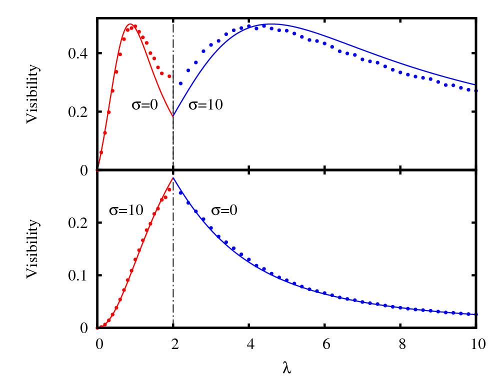
Figure 4: (Color online) Visibility of the oscillations in real and quasi-momentum space a function $\lambda$, for $\varphi=0$. The numerical points are compared with the three-mode approximation (full lines). Bottom: only few modes have been initially populated by using a $\delta$-function initial wave packet in real space and a Gaussian with $\sigma=10$ in momentum space. Top: many modes have been initially populated by inverting the initial conditions with respect to the bottom panel.

In the region $\lambda>2$ the few-mode approximation is expected to fail in the quasi-momentum space, where the wave packet is no more localized. Indeed, in this regime, we do not see any significant evidence of periodic behaviors in the quasi-momentum distribution (see the bottom panel of Fig. 1). Conversely, owing to the duality of the AA model, one expects periodic oscillations to take place in real space, where the wave packet is localized. This is confirmed by our numerical integration of Eq. (1), as shown in Fig. 3. In the top panel the wave packed spreads ballistically and one cannot detect any significant periodic behaviour; conversely in the bottom panel the wave packet is localized, while the central peak and its nearest neighbours oscillate periodically. By assuming that the initial density distribution is localized in a single lattice site, $n=0$, which is coupled with the nearest neighboring sites, $n=\pm 1$, we obtain a three-mode approximation analogous to the one used before in quasi-momentum space, but describing oscillations in the spatial distribution. The scenario in real space is more complicated because one generally observes oscillations with several frequency components, which also depend on the phase $\varphi$. However, in the special case $\varphi=0$, one finds just a single frequency, given by

$$\nu(\lambda>2)=(2\pi)^{-1}\sqrt{\lambda^{2}[1-\cos(2\pi\alpha)]^{2}+8}\,,$$ (7)

which is shown as the solid line for $\lambda>2$ in Fig. 2. In the same figure we also plot the frequency obtained from the full numerical integration of Eq. (1) (blue dots in the $\lambda>2$ region); in this calculation we have used a Gaussian of width $\sigma=10$ as initial shape of the wave packet, but we have also checked that the frequency $\nu$ does not depend on $\sigma$, except close to $\lambda=2$. The dashed line is the result of a straightforward semi-analytic extension to five modes, as in the $\lambda<2$ region. It is worth stressing that the condition for the validity of the few-mode approximation for the oscillations in real space ($\psi_{n}=\delta_{n,0}$ or, equivalently, $\sigma\lesssim 1$) is much more constraining than the one in momentum space ($1/{\sigma}\lesssim 2\pi\alpha$) from the point of view of experimental realization.

The amplitude of the oscillations in both real and momentum space also changes with $\lambda$, affecting its visibility. The latter can be calculated from the frequency spectrum of the numerical solution of Eq. (1), as the ratio between the modulus of the Fourier component of frequency $\nu(\lambda)$ and the modulus of the component at zero frequency. In a consistent way, one can define the visibility in the three-mode approximation; for the oscillations in momentum space for $\lambda<2$, the visibility can be written as $(1/2)\gamma_{1}\gamma_{2}g_{0,1}g_{0,2}/[(\gamma_{1}g_{0,1})^{2}+(\gamma_{2}g_{0,2})^{2}]$. A similar definition can be given in real space for $\lambda>2$. In Fig. 4 we show the visibility of the oscillations as a function of $\lambda$. The points are the numerical results, while the lines represent the three-mode approximation. We have used two values for the width of the initial Gaussian wave packet, namely $\sigma=0$ (i.e., a $\delta$-function) and $\sigma=10$. In the upper panel, the two values of $\sigma$ are used for $\lambda<2$ and $\lambda>2$, respectively. They correspond to a broad initial wave packet both in momentum space for $\lambda<2$ and real space for $\lambda>2$. In the bottom panel we use again the same values of $\sigma$, but in the opposite regions, so to have a narrow initial wave packet in both spaces (width, ). One can see that the visibility depends significantly on both $\sigma$ and $\lambda$. Again, the three-mode approximation is qualitatively correct, except near $\lambda=2$. We observe that the three-mode approximation gives a better agreement for a narrow initial distribution (lower panel), as in the opposite case of a broad distribution many modes are initially excited and this approximation is not expected to be accurate. Another interesting feature is the effect of the duality of the AA model. Indeed, in both panels, the results in the region $\lambda<2$ almost coincide with those in the region $\lambda>2$ under the change of variable $\lambda\to 4/\lambda$, provided the initial distributions are broad (upper panel) or narrow (lower panel) in both momentum and real spaces; this duality also implies the continuity at $\lambda=2$.

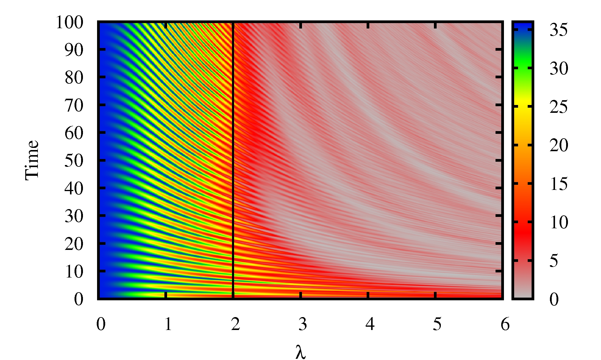
Figure 5: (Color online) Phase-averaged intensity of the central peak in momentum space, $|f_{0}(t)|^{2}$, as a function of time and disorder strength $\lambda$ for a wavepacket with $\sigma=10$. The intensity is given in arbitrary units.

IV Summary

We have shown that the time evolution of a wave packet in the Aubry-André model exhibits interesting periodic behaviors both in momentum space, for $\lambda<2$, and in real space, for $\lambda>2$. The occurrence of oscillations in the momentum and density distributions can be used to test the applicability of the AA model to the description of the dynamics of ultracold gases in 1D bichromatic lattices. We have numerically calculated the frequency and visibility of these oscillations and we have introduced a simple few-mode approximation to interpret their behavior. The use of momentum space has some important advantages. First, the frequency of the oscillations does not depend on the relative phase $\varphi$ of the two lattices or, in other terms, on the initial position of the wave packet, which would be hardly controllable in typical experiments. Second, the condition for the applicability of a few-mode approximation is less restrictive than in real space, because the width of the initial wave packet in momentum space can be easily made much smaller than the distance between the modes which are coupled in time evolution.

Our analysis suggests that the oscillations of the central and side peaks in the momentum distribution can be efficiently used to probe the transition from diffusion to localization in the AA model. A possible strategy consists of measuring the intensity of the central peak as a function of time for different values of $\lambda$, exploiting the fact that for $\lambda>2$ the oscillations are phase dependent, while for $\lambda<2$ they are not. Actually, in typical experiments with ultracold atoms, the phase $\varphi$ varies at random at each realization, so that performing an average over many realizations at fixed $\lambda$ is equivalent to an average over numerical simulations with different $\varphi$. Thus one expect that the oscillations vanish for $\lambda>2$ (phase sensitive regime), but remain clearly visible for $\lambda<2$ (phase independent regime). This is shown in Fig. 5, where the average has been done over $50$ different values of the phase $\varphi$ for each value of $\lambda$. Indeed the behavior of $|f_{0}(t)|^{2}$ exhibits a transition at $\lambda=2$. From the same figure one can also extract the frequency $\nu(\lambda<2)$. By using the experimental parameters of Ref. deissler2010 , with $\alpha=1064.4/866.6$ and $\lambda=1$, the oscillation period turns out to be of the order of $5$ ms.

These results are relevant for current experiments with ultracold atoms, where the momentum distribution can be detected with good resolution by performing time of flight measurements. This study provides also a starting point for future investigations on the interplay between interaction and localization. It is known that in certain regimes the presence of a repulsive interaction can destroy the disorder induced (Anderson) localization giving a sub-diffusive spreading of an initially localized wavepacket (larcher2009, ; interaction_vs_localization, ), but its experimental detection in real space is currently limited by the difficulty to reach the long time regime, and by the finite resolution in the observation of low density tails of the atomic distribution deissler2010 . In this sense, the observation of oscillations in momentum space can be a more reliable tool.

Acknowledgments. M.M. acknowledges support from INO-CNR through the DQS EuroQUAM  project from ESF. This work is also supported by Miur.

References

- (1) B. Kramer and A. MacKinnon, Rep. Prog. Phys. 56 1469 (1993).
- (2) P. W. Anderson, Phys. Rev. 109, 1492 (1958).
- (3) L. Fallani, C. Fort, M. Inguscio, Adv. At. Mol. Opt. Phys. 56, 119(2008).
- (4) J. Billy, V. Josse, Z. Zuo, A. Bernard, B. Hambrecht, P. Lugan, D. Clément, L. Sanchez-Palencia, P. Bouyer and, A. Aspect, Nature 453, 891 (2008).
- (5) G. Roati, C. D’Errico, L. Fallani, M. Fattori, C. Fort, M. Zaccanti, G. Modugno, M. Modugno and, M. Inguscio, Nature 453, 895 (2008).
- (6) B. Deissler, M. Zaccanti, G. Roati, C. D’Errico, M. Fattori, M. Modugno, G. Modugno, and M. Inguscio, Nat. Phys. 6, 354 (2010).
- (7) M. Pasienski, D. McKay, M. White, B. DeMarco, Nat. Phys. 6, 677 (2010).
- (8) P. G. Harper, Proc. Phys. Soc. London A 68, 874 (1955).
- (9) S. Aubry and G. André, Ann. Israel Phys. Soc. 3, 133 (1980).
- (10) M. Larcher, F. Dalfovo, and M. Modugno, Phys. Rev. A 80, 053606 (2009).
- (11) A. S. Pikovsky and D. L. Shepelyansky, Phys. Rev. Lett. 100, 094101 (2008); I. García-Mata and D. L. Shepelyansky, Phys. Rev. E 79, 026205 (2009); S. Flach, D. O. Krimer and, Ch. Skokos, Phys. Rev. Lett. 102, 024101 (2009); Ch. Skokos, D. O. Krimer, S. Komineas and, S. Flach, Phys. Rev. E 79, 056211 (2009).
- (12) G.S. Ng and T.Kottos, Phys. Rev. B 75, 205120 (2007); G. Kopidakis, S. Komineas, S. Flach, and S. Aubry, Phys. Rev. Lett. 100, 084103 (2008); X. Deng, R. Citro, E. Orignac, and A. Minguzzi , Eur. Phys. J. B 68, 435 (2009). S. K. Adhikari and L. Salasnich, Phys. Rev. A 80, 023606 (2009); Y. Shikano and H. Katsura, Phys. Rev. E 82, 031122 (2010).
- (13) C. Aulbach, A. Wobst, G.-L. Inglold, P. Hänggi and, I. Varga, New J. Phys. 6, 70 (2004).
- (14) The AA model has been experimentally realized also with light diffusion in photonic lattices, in Y. Lahini, R. Pugatch, F. Pozzi, M. Sorel, R. Morandotti, N. Davidson, and Y. Silberberg, Phys. Rev. Lett. 103, 013901 (2009).
- (15) H. Hiramoto and S. Abe, J. Phys. Soc. Japan 57, 1365 (1988).
- (16) M. Modugno, New J. Phys. 11, 033023 (2009).
- (17) Eq. (1) is solved by means of a RK4 method. See e.g., W. H. Press, S. Teukolsky, W. Vetterling, and B. Flannery, Numerical Recipes (Cambridge University Press, New York, 1986).
- (18) The frequency is extracted from the frequency spectrum of the central peak in quasi-momentum (real) space, (). The signal is Fourier transformed, and the oscillation frequency is identified as the dominant component of the frequency spectrum.
- (19) For , the momentum width is much smaller than the distance between coupled modes, .