Steady Homogeneous Turbulence in the Presence of an Average Velocity Gradient

Abstract

We study the homogeneous turbulence in the presence of a constant average velocity gradient in an infinite fluid domain, with a novel finite-scale Lyapunov analysis, presented in a previous work dealing with the homogeneous isotropic turbulence.

Here, the energy spectrum is studied introducing the spherical averaged pair correlation function, whereas the anisotropy caused by the velocity gradient is analyzed using the equation of the two points velocity distribution function which is determined through the Liouville theorem. As a result, we obtain the evolution equation of this velocity correlation function which is shown to be valid also when the fluid motion is referred with respect to a rotating reference frame. This equation tends to the classical von Kármán-Howarth equation when the average velocity gradient vanishes.

We show that, the steady energy spectrum, instead of following the Kolmogorov law $\kappa^{-5/3}$, varies as $\kappa^{-2}$. Accordingly, the structure function of the longitudinal velocity difference $\langle\Delta u_{r}^{n}\rangle\approx r^{\zeta_{n}}$ exhibits the anomalous scaling $\zeta_{n}\approx n/2$, and the integral scales of the correlation function are much smaller than those of the isotropic turbulence.

1 Introduction

Although the Kolmogorov law $E(\kappa)\approx k^{-5/3}$ represents the main result of the isotropic turbulence, there are many experimental evidences and theoretical arguments indicating that this is not the only spectrum observed in the fully developed turbulence of incompressible fluids (Brissaud et al (1973), Moffat (1978), Gordienko et al (2001), Baroud et al (2002)).

For example, in Brissaud et al (1973) and Moffat (1978), it is shown through the dimensional analysis, that the energy spectrum in the presence of an average velocity gradient $\partial U/\partial y$ can follow the law $\approx k^{-7/3}$ in the inertial subrange. This is a particular result arising from the assumption that the energy spectrum is linear in $\partial U/\partial y$. More in general, assuming that the energy spectrum is proportional to $(\partial U/\partial y)^{\beta}$ with $\beta>0$, the Buckingham theorem states that $E(\kappa)\approx\kappa^{-5/3-2/3\beta}$, and different scaling exponent are possible.

Gordienko et al (2001) studied the forced driving turbulence, where the forcing term can have various origins. The authors remarked that there are two dimensionless parameters, characterizing the forcing term, which influence the shape of the energy spectrum and are responsible for the anomalous spectra. They showed that, in a certain interval of variation of one of these parameters, the spectrum follows the Kolmogorov law, whereas for an opportune choice of it, the spectrum behaves like $\kappa^{-2}$ in the inertial subrange.

These different scaling are caused by the shear rate which leads to the development of coherent fluid structures. These are streaky structures, due to the stretching of the vortex lines, which exhibit the maximum dimension along the stream direction (Lee, Kim & Moin (1990)). In Ref. (Lee, Kim & Moin (1990)), the authors remark that these streaky structures influence the spanwise correlation of streamwise velocity components, being a non monotonic function which becomes negative at high values of the spanwise distances.

Further, in Baroud et al (2002), the authors experimentally analyzed the statistics of the longitudinal velocity difference $\Delta u_{r}$ in a closed cylindric tank which rotates around its symmetry axis at a given spin rate. The turbulence is generated by pumping the flow in the tank through two concentric rings of 120 holes each, placed at the bottom of the tank, where the source ring is the internal one. This generates an average radial flow that, combined with the spin rate, determines a Coriolis force whose magnitude varies with the distance from the rotation axis. As a consequence, a counterrotating flow and an average velocity gradient with respect to the tank frame is observed (Baroud et al (2002)). The authors found that $\Delta u_{r}$ presents the anomalous scaling $\langle\Delta u_{r}^{n}\rangle\approx r^{\zeta_{n}}$ with $\zeta_{n}\simeq n/2$, in contrast with the Kolmogorov law ($\zeta_{n}\simeq n/3$), and that $E(\kappa)\approx\kappa^{-2}$.

The present work studies the homogeneous turbulence in an infinite fluid domain in the presence of an average velocity gradient $\nabla_{\bf x}{\bf U}$, using the finite-scale Lyapunov analysis, proposed by de Divitiis (2010), de Divitiis (2011) for studying the homogeneous isotropic turbulence.

In the first section, we define the spherical part of the velocity correlation tensor $R_{ij}$, and we derive the evolution equation for $R_{ii}$ from the Navier-Stokes equation with $\nabla_{\bf x}{\bf U}\neq\bf 0$.

To study the effect of $\nabla_{\bf x}{\bf U}$ on the anisotropy and on $R_{ij}$, the evolution equation for the pair distribution function is derived from the Liouville theorem, assuming that the statistical equilibrium corresponds to the condition of isotropic turbulence when the kinetic energy rate is equal to zero. From this equation, the steady velocity correlation tensor is expressed in function of the average velocity gradient and of the maximal finite-scale Lyapunov exponent and, in particular, the Boussinesq closure for the Reynolds stress is obtained.

Finally, the equation for the spherical averaged longitudinal correlation function is determined, whose solutions depend on the average velocity gradient. Moreover, we show that this equation is still valid when the fluid motion is refereed with respect to a non-inertial rotating frame of reference. The steady solutions of this equation are numerically calculated for different Taylor-Scale Reynolds number and several results are presented. We found that $E(\kappa)\approx\kappa^{-2}$ in the inertial subrange, thus the statistical moments $\langle\Delta u_{r}^{n}\rangle\approx r^{\zeta_{n}}$ exhibit the anomalous scaling $\zeta_{n}\approx n/2$, whereas the integral scales of the longitudinal correlation function are much lesser than those of the isotropic turbulence. In the case of homogeneous turbulence in the presence of a steady shear rate, the spanwise correlation function of the streamwise velocity component is also calculated.

2 Analysis

This section analyzes the homogeneous turbulence with an uniform average velocity gradient $\nabla_{\bf x}{\bf U}$.

The fluid velocity, measured in the reference frame $\Re$, is ${\bf v}={\bf U}+{\bf u}$, where ${\bf U}\equiv(U_{x},U_{y},U_{z})$ and ${\bf u}\equiv(u_{x},u_{y},u_{z})$ are, average and fluctuating velocity, respectively. The velocity correlation tensor is defined as $R_{ij}=\langle u_{i}u^{\prime}_{j}\rangle$, being $u_{i}$ and $u^{\prime}_{j}$ the velocity components of $\bf u$ calculated at $\bf x$ and ${\bf x^{\prime}}={\bf x}+{\bf r}$, where the brackets denote the average on the statistical ensemble of $\bf u$ and $\bf u^{\prime}$, and $\bf r$ is the separation distance (Kármán-Howarth (1938), Batchelor (1953)).

In order to determine the evolution equation of $R_{ij}$, we start from the Navier-Stokes equations, written for the fluctuating velocity (Batchelor (1953)), in the points ${\bf x}$ and ${\bf x}^{\prime}$

$$\begin{array}[]{l@{\hspace{+0.2cm}}l}\displaystyle\frac{\partial u_{i}}{\partial t}=-\frac{\partial u_{i}u_{k}}{\partial x_{k}}-\frac{\partial U_{i}u_{k}}{\partial x_{k}}-\frac{\partial u_{i}U_{k}}{\partial x_{k}}-\frac{1}{\rho}\frac{\partial p}{\partial x_{i}}+\nu\nabla^{2}u_{i}\hfil\hskip 5.69046pt\\ \hfil\hskip 5.69046pt\\ \displaystyle\frac{\partial u^{\prime}_{j}}{\partial t}=-\frac{\partial u^{\prime}_{j}u^{\prime}_{k}}{\partial x^{\prime}_{k}}-\frac{\partial U^{\prime}_{j}u^{\prime}_{k}}{\partial x^{\prime}_{k}}-\frac{\partial u^{\prime}_{j}U^{\prime}_{k}}{\partial x^{\prime}_{k}}-\frac{1}{\rho}\frac{\partial p^{\prime}}{\partial x^{\prime}_{j}}+\nu\nabla^{\prime 2}u^{\prime}_{j}\hfil\hskip 5.69046pt\end{array}$$ (4)

where $p$ is the fluctuating pressure and ${\bf U}^{\prime}$ is

$${\bf U}^{\prime}={\bf U}+\nabla_{\bf x}{\bf U}\ {\bf r}$$ (5)

being ${\bf U}$ and $\nabla_{\bf x}{\bf U}$ assigned quantities. The repeated index indicates the summation with respect the same index. The evolution equation of $R_{ij}$ is determined by multiplying first and second equation by $u^{\prime}_{j}$ and $u_{i}$, respectively, summing the so obtained equations, and calculating the average on the statistical ensemble (Batchelor (1953)):

$$\displaystyle\frac{\partial R_{ij}}{\partial t}=T_{ij}+P_{ij}+2\nu\nabla^{2}R_{ij}-\frac{\partial U_{i}}{\partial x_{k}}R_{kj}-\frac{\partial U_{j}}{\partial x_{k}}R_{ik}+\frac{\partial R_{ij}}{\partial r_{k}}(U_{k}-U_{k}^{\prime})$$ (6)

being

$$\begin{array}[]{l@{\hspace{+0.2cm}}l}\displaystyle T_{ij}({\bf r})=\frac{\partial}{\partial r_{k}}\left\langle u_{i}u_{j}^{\prime}(u_{k}-u_{k}^{\prime})\right\rangle,\ \ \ \ \displaystyle P_{ij}({\bf r})=\frac{1}{\rho}\left(\frac{\partial\langle pu^{\prime}_{j}\rangle}{\partial r_{i}}-\frac{\partial\langle p^{\prime}u_{i}\rangle}{\partial r_{j}}\right)\hfil\hskip 5.69046pt\end{array}$$ (8)

where $\partial\langle...\rangle/\partial x_{i}\equiv-\partial\langle...\rangle/\partial r_{i}$ and $\partial\langle...\rangle/\partial x^{\prime}_{i}\equiv\partial\langle...\rangle/\partial r_{i}$. Making the trace of Eq. (6), we obtain the following scalar equation

$$\displaystyle\frac{\partial R}{\partial t}=\frac{1}{2}H+2\nu\nabla^{2}R-\frac{\partial U_{i}}{\partial x_{k}}R_{ik}^{S}+\frac{\partial R}{\partial r_{k}}(U_{k}-U_{k}^{\prime})$$ (9)

where $R_{ik}^{S}$ is the symmetric part of $R_{ik}$, and $R$, defined as

$$\displaystyle R=\frac{1}{2}{R_{ii}},$$ (10)

gives the turbulent kinetic energy for ${\bf r}$=$0$, $H$ $\equiv$ $T_{ii}$ provides the mechanism of energy cascade, and $P_{ii}({\bf r})\equiv 0$ arises from the fluid incompressibility (Kármán-Howarth (1938), Batchelor (1953)).

Equation (9) incudes two additional terms with respect to the homogeneous isotropic turbulence. $-{\partial U_{i}}/{\partial r_{k}}R_{ik}$ corresponds to the kinetic energy production if $-{\partial U_{i}}/{\partial r_{k}}R_{ik}(0)>0$, whereas ${\partial R_{ii}}/{\partial r_{k}}(U_{k}-U_{k}^{\prime})$ represents an energy transfer as this latter vanishes for ${\bf r}=0$.

Assuming the condition of isotropic turbulence, $\partial U_{i}/\partial x_{k}R_{ki}$ does not give energy production, and the flow corresponds to a dying turbulence whose dissipation rate is calculated with the von Kármán-Howarth equation. In this case the energy spectrum is a function of $\mbox{\boldmath$\kappa$}^{2}\equiv\kappa_{i}\kappa_{i}$.

On the contrary, the combined effect of the anisotropy (i.e. $\langle u_{x}^{2}\rangle$ $\neq$ $\langle u_{y}^{2}\rangle$, $\langle u_{x}^{2}\rangle$ $\neq$ $\langle u_{z}^{2}\rangle$, $R_{ki}(0)$ $\neq$ 0, $i\neq k$) and of $\nabla_{\bf x}{\bf U}$ leads to the following condition

$$\displaystyle\frac{\partial U_{i}}{\partial x_{k}}R_{ki}(0)\neq 0$$ (11)

which can correspond to an energy production, where the energy spectrum is not more a function of $\mbox{\boldmath$\kappa$}^{2}$.

At this point, we want to determine an useful scalar equation for describing the main properties of the velocity correlation. We start decomposing $R_{ij}$, $H$ and $\bf U$ into an even function of $r\equiv|{\bf r}|$ (here called spherical part), plus the remaining term:

$$\begin{array}[]{l@{\hspace{+0.2cm}}l}R_{ij}(r_{x},r_{y},r_{z})=\hat{R}_{ij}(r)+\Delta R_{ij}(r_{x},r_{y},r_{z})\hfil\hskip 5.69046pt\\ \hfil\hskip 5.69046pt\\ H(r_{x},r_{y},r_{z})=\hat{H}(r)+\Delta H(r_{x},r_{y},r_{z})\hfil\hskip 5.69046pt\\ \hfil\hskip 5.69046pt\\ {\bf U}^{\prime}-{\bf U}=\hat{\bf U}(r)+\Delta{\bf U}(r_{x},r_{y},r_{z})\hfil\hskip 5.69046pt\end{array}$$ (17)

being

$$\begin{array}[]{l@{\hspace{+0.99cm}}l}\displaystyle\hat{R}_{ij}(r)=\frac{1}{6}\left(R_{ij}(r,0,0)+R_{ij}(0,r,0)+R_{ij}(0,0,r)\right)\hfil\hskip 28.16838pt\\ \hfil\hskip 28.16838pt\\ \displaystyle+\frac{1}{6}\left(R_{ij}(-r,0,0)+R_{ij}(0,-r,0)+R_{ij}(0,0,-r)\right),\hfil\hskip 28.16838pt\\ \hfil\hskip 28.16838pt\\ \displaystyle\hat{H}(r)=\frac{1}{6}\left(H(r,0,0)+H(0,r,0)+H(0,0,r)\right)\hfil\hskip 28.16838pt\\ \hfil\hskip 28.16838pt\\ \displaystyle+\frac{1}{6}\left(H(-r,0,0)+H(0,-r,0)+H(0,0,-r)\right),\hfil\hskip 28.16838pt\\ \hfil\hskip 28.16838pt\\ \displaystyle\hat{\bf U}(r)=\frac{1}{6}\left({\bf U}(r,0,0)+{\bf U}(0,r,0)+{\bf U}(0,0,r)\right)\hfil\hskip 28.16838pt\\ \hfil\hskip 28.16838pt\\ \displaystyle+\frac{1}{6}\left({\bf U}(-r,0,0)+{\bf U}(0,-r,0)+{\bf U}(0,0,-r)\right)\hfil\hskip 28.16838pt\end{array}$$ (29)

where $\Delta R_{ij}({\bf 0})$=$\Delta H({\bf 0})$ = 0. Therefore, the Fourier transform of $\hat{R}$ identifies the part of the energy spectrum depending upon $\mbox{\boldmath$\kappa$}^{2}$ whose integral over the Fourier space gives the whole turbulent kinetic energy. Moreover, $\hat{\bf U}\equiv 0$ and $\Delta{\bf U}\equiv{\bf U}^{\prime}-{\bf U}$.

The laplacian of $R$ appearing into Eq. (9) is written taking into account Eqs. (17)

$$\nabla^{2}R=\frac{\partial^{2}\hat{R}}{\partial r^{2}}+\displaystyle\frac{2}{r}\frac{\partial\hat{R}}{\partial r}+\nabla^{2}\Delta R$$ (30)

Substituting Eqs. (17), (29), (30) into Eq. (9), we obtain the following equation

$$\displaystyle\frac{\partial\hat{R}}{\partial t}+\frac{\partial\Delta R}{\partial t}=\frac{1}{2}\hat{H}+\frac{1}{2}\Delta H+2\nu\left(\frac{\partial^{2}\hat{R}}{\partial r^{2}}+\displaystyle\frac{2}{r}\frac{\partial\hat{R}}{\partial r}\right)+2\nu\nabla^{2}\Delta R-\hat{G}-\Delta{G}$$ (31)

where

$$\begin{array}[]{l@{\hspace{+0.2cm}}l}\displaystyle\hat{G}=\frac{\partial U_{i}}{\partial x_{k}}\hat{R}_{ki}+\hat{G}_{0},\ \ \ \ \displaystyle\Delta{G}=\frac{\partial U_{i}}{\partial x_{k}}\Delta{R}_{ki}-\Delta\left(\frac{\partial R}{\partial r_{k}}(U_{k}-U_{k}^{\prime})\right)\hfil\hskip 5.69046pt\end{array}$$ (33)

where $\hat{G}_{0}$ represents the spherical part of $-\partial R/\partial r_{k}(U_{k}-U_{k}^{\prime})$. As $\hat{R}$, $\hat{H}$ and $\hat{G}$ are even functions of $r$, whereas $\Delta{R}$, $\Delta{H}$ and $\Delta{G}$ are not, and since Eq. (31) must be satisfied at each time and for all the values of $\bf r$, Eq. (31) is satisfied when

$$\begin{array}[]{l@{\hspace{+0.2cm}}l}\displaystyle\frac{\partial\hat{R}}{\partial t}=\frac{\hat{H}}{2}+2\nu\left(\frac{\partial^{2}\hat{R}}{\partial r^{2}}+\displaystyle\frac{2}{r}\frac{\partial\hat{R}}{\partial r}\right)-\hat{G}\hfil\hskip 5.69046pt\end{array}$$ (35)

$$\begin{array}[]{l@{\hspace{+0.2cm}}l}\displaystyle\frac{\partial\Delta R}{\partial t}=\frac{\Delta H}{2}+2\nu\nabla^{2}\Delta R-\Delta{G}\hfil\hskip 5.69046pt\end{array}$$ (37)

Thanks to decomposition (17), Eq. (35) is about independent from Eq. (37), thus $\hat{R}$ is governed by a decoupled scalar equation which individually describes some of the properties of the non-isotropic turbulence related to $\hat{R}(r)$. As far as Eq. (37) is concerned, $\Delta R$ is a complicate function of $\bf r$ and $t$ which depends on the particular problem.

Here, the turbulence is studied using Eq. (35) alone, whereas $R_{ij}({\bf r})$ will be determined in function of $\nabla_{\bf x}{\bf U}$, by means of a proper statistical analysis of the two-points velocity correlation.

3 Two-points distribution function

In order to obtain the pair distribution function, consider the equations of motion of the various continuum fluid particles

$$\displaystyle\frac{d{\bf x}_{k}}{dt}={\bf v}({{\bf x}_{k}},t)\equiv{\bf v}_{k},\ \ k=1,2,...N$$ (38)

This is an ordinary differential system, where ${\bf v}({{\bf x}},t)$ varies according to the Navier-Stokes equations, here written for each fluid particle in the following form

$$\displaystyle\frac{d{\bf v}_{k}}{dt}=\dot{\bf v}_{k}({\bf v}_{1},{\bf v}_{2},...,{\bf v}_{k},...,{\bf v}_{N}),\ k=1,2,...,N$$ (39)

being $\dot{\bf v}_{k}$ the acceleration of the $k^{th}$ particle. This form of the Navier-Stokes equations is obtained once the pressure is eliminated through the continuity equation.

The distribution function of the velocities and of the spatial coordinates of all the fluid particles

$$F=F(t,{\bf x}_{1},{\bf x}_{2},...{\bf x}_{N},{\bf v}_{1},{\bf v}_{2},...{\bf v}_{N})$$ (40)

is defined in the phase space $\Gamma\equiv\Gamma_{1}\times\Gamma_{2}\times...\times\Gamma_{N}$, where $\Gamma_{k}=\left\{{\bf x}_{k}\right\}\times\left\{{\bf v}_{k}\right\}$, $k=1,2,...N$, being $\left\{{\bf x}_{k}\right\}$ = $\left\{(-\infty,\infty)\times(-\infty,\infty)\times(-\infty,\infty)\right\}$ and $\left\{{\bf v}_{k}\right\}$ = $\left\{(-\infty,\infty)\times(-\infty,\infty)\times(-\infty,\infty)\right\}$ the subspaces of coordinates and velocities described by the $k^{th}$ particle. This function, which vanishes on the boundaries of $\left\{{\bf v}_{k}\right\}$, ($k=1,2,...N$), satisfies the Liouville theorem associated to Eqs. (38) and (39) (Nicolis (1995))

$$\displaystyle\frac{\partial F}{\partial t}+\sum_{k=1}^{N}\nabla_{{\bf x}_{k}}F\cdot{\bf v}_{k}=-\sum_{k=1}^{N}\nabla_{{\bf v}_{k}}F\cdot\dot{\bf v}_{k}$$ (41)

To study the correlation between two points of space ${\bf x}\equiv{\bf x}_{1}$ and ${\bf x}^{\prime}\equiv{\bf x}_{2}$, the two-points distribution function $F^{(2)}$ associated to ${\bf x}$ and ${\bf x}^{\prime}$, is considered. This is the reduced distribution function calculated, by definition, integrating $F$ over $\Gamma_{3}\times\Gamma_{4}\times...\times\Gamma_{N}$

$$F^{(2)}=\int_{\Gamma_{3}}\int_{\Gamma_{4}}...\int_{\Gamma_{N}}F\prod_{k=3}^{N}dx^{3}_{k}dv^{3}_{k}$$ (42)

Hence, $F^{(2)}$ obeys to the equation arising from Eq. (41)

$$\displaystyle\frac{\partial F^{(2)}}{\partial t}+\nabla_{{\bf x}}F^{(2)}\cdot{\bf v}+\nabla_{{\bf x}^{\prime}}F^{(2)}\cdot{\bf v}^{\prime}=J$$ (43)

where

$$J=-\int_{\Gamma_{3}}\int_{\Gamma_{4}}...\int_{\Gamma_{N}}\left(\sum_{k=3}^{N}\nabla_{{\bf x}_{k}}F\cdot{\bf v}_{k}+\sum_{k=1}^{N}\nabla_{{\bf v}_{k}}F\cdot\dot{\bf v}_{k}\right)\prod_{k=3}^{N}dx^{3}_{k}dv^{3}_{k}$$ (44)

is the rate of $F^{(2)}$ caused by the interactions between the two particles that simultaneously pass through $\bf x$ and $\bf x^{\prime}$, and all the other fluid particles.

The local statistical equilibrium for the system of two fluid particles is expressed by the condition

$$J=0$$ (45)

To determine the expression of $J$, the case with null rate of kinetic energy is first considered. We assume that the local statistical equilibrium corresponds to the condition of fully developed homogeneous isotropic turbulence in an infinite fluid domain whose values of momentum and kinetic energy coincide with those of the current condition

$$\begin{array}[]{l@{\hspace{+0.2cm}}l}\displaystyle\int_{v}\int_{v^{\prime}}F^{(2)}du^{3}du^{\prime 3}=\displaystyle\int_{v}\int_{v^{\prime}}F^{(2)}_{0}du^{3}du^{\prime 3},\hfil\hskip 5.69046pt\\ \hfil\hskip 5.69046pt\\ \displaystyle\int_{v}\int_{v^{\prime}}F^{(2)}{\bf u}\ du^{3}du^{\prime 3}=\displaystyle\int_{v}\int_{v^{\prime}}F^{(2)}_{0}{\bf u}\ du^{3}du^{\prime 3},\hfil\hskip 5.69046pt\\ \hfil\hskip 5.69046pt\\ \displaystyle\int_{v}\int_{v^{\prime}}F^{(2)}{\bf u}\cdot{\bf u}\ du^{3}du^{\prime 3}=\displaystyle\int_{v}\int_{v^{\prime}}F^{(2)}_{0}{\bf u}\cdot{\bf u}\ du^{3}du^{\prime 3}\hfil\hskip 5.69046pt\end{array}$$ (51)

That is, $F^{(2)}_{0}$ represents the fully developed isotropic turbulence and is related to $F^{(2)}$ through Eqs. (51). Taking into account the homogeneity, the centered moments of $F^{(2)}_{0}$ are constants in space, thus $F^{(2)}_{0}$ is a function of ${\bf v}-{\bf U}$ and ${\bf v}^{\prime}-{\bf U}^{\prime}$

$$F^{(2)}_{0}({\bf v},{\bf v}^{\prime};{\bf x},{\bf x}^{\prime})=F^{(2)}_{0}({\bf v}-{\bf U}({\bf x}),{\bf v}^{\prime}-{\bf U}({\bf x}^{\prime}))$$ (52)

Now, $J$ is the rate of $F^{(2)}({\bf u},{\bf u}^{\prime})$ whose variations are caused by the fluctuations ($\tilde{\bf u}$, $\tilde{\bf u}^{\prime}$)

$$\displaystyle J\equiv\left(\frac{dF^{(2)}}{dt}\right)_{\bf\tilde{\bf u},\tilde{\bf u}^{\prime}}$$ (53)

These variations are determined using the finite scale Lyapunov analysis presented in de Divitiis (2010), where for sake of convenience, $J$ is calculated for $\bf\tilde{\bf u}$=0, $\displaystyle\bf\tilde{\bf u}^{\prime}=\tilde{\bf u}^{\prime}_{0}{\mbox{e}}^{\lambda(r)t}$. According to the theory, $|{\bf\tilde{\bf u}^{\prime}_{0}}|<<|{\bf u}^{\prime}|$, and the variations of $F^{(2)}$ are calculated through $F^{(2)}_{0}$ and the Frobenius-Perron equation (Nicolis (1995))

$$\begin{array}[]{l@{\hspace{+0.2cm}}l}\displaystyle F^{(2)}({\bf u},{\bf u}^{\prime}+\tilde{\bf u}^{\prime},t)=\int_{-\infty}^{\infty}\int_{-\infty}^{\infty}\int_{-\infty}^{\infty}F^{(2)}_{0}({\bf u},{\bf u}^{\prime}+\tilde{\bf u}^{\prime}_{0})\delta(\tilde{\bf u}^{\prime}-\tilde{\bf u}^{\prime}_{0}{\mbox{e}}^{\lambda(r)t})d^{3}u^{\prime}\hfil\hskip 5.69046pt\\ \hfil\hskip 5.69046pt\\ =F^{(2)}_{0}({\bf u},{\bf u}^{\prime}+\tilde{\bf u}^{\prime}{\mbox{e}}^{-\lambda(r)t})\hfil\hskip 5.69046pt\end{array}$$ (57)

where $\delta$ is the Dirac delta and $\lambda(r)>0$ is the maximal Lyapunov exponent of finite scale (de Divitiis (2010)). Being $|\tilde{\bf u}^{\prime}{\mbox{e}}^{-\lambda(r)t}|<<|{\bf u}^{\prime}|$

$$\displaystyle F^{(2)}_{0}({\bf u},{\bf u}^{\prime}+\tilde{\bf u}^{\prime}{\mbox{e}}^{-\lambda(r)t})\simeq\displaystyle F^{(2)}_{0}({\bf u},{\bf u}^{\prime})+\frac{\partial F^{(2)}_{0}}{\partial{\bf u}^{\prime}}\cdot\tilde{\bf u}^{\prime}{\mbox{e}}^{-\lambda(r)t}$$ (58)

and, taking into account Eqs. (57) and (58), $J=\lambda(r)(F^{(2)}_{0}-F^{(2)})$.

In presence of a nonzero rate of kinetic energy, $J$ reads as

$$\displaystyle J=\lambda(r)\left(F^{(2)}_{0}-F^{(2)}\right)-J_{D}$$ (59)

where $-J_{D}$ is the rate of $F^{(2)}$ due to the rate of kinetic energy. Now, the statistical equilibrium ($J=0$) differs from the isotropic turbulence, being $J_{D}\neq$0 into Eq. (59).

Therefore, the evolution equation of $F^{(2)}$ is assumed to be

$$\displaystyle\frac{\partial F^{(2)}}{\partial t}+\nabla_{{\bf x}}F^{(2)}\cdot{\bf v}+\nabla_{{\bf x}^{\prime}}F^{(2)}\cdot{\bf v}^{\prime}=\lambda(r)\left(F^{(2)}_{0}-F^{(2)}\right)-J_{D}$$ (60)

Accordingly, $F^{(2)}$ varies depending on the boundary conditions associated to Eq. (60) and on the initial condition. Equation (60) is a partial differential equation, where $1/\lambda$ identifies the relaxation time of the system given by a pair of fluid particles.

4 Effect of the average velocity gradient

To study the effect of $\nabla_{\bf x}{\bf U}$, consider now the homogeneous turbulence in a steady velocity gradient, whose pair distribution function is

$$F^{(2)}({\bf v},{\bf v}^{\prime};{\bf x},{\bf x}^{\prime})=F^{(2)}_{0}({\bf v}-{\bf U}({\bf x}),{\bf v}^{\prime}-{\bf U}({\bf x}^{\prime}))+\phi^{(2)}({\bf v},{\bf v}^{\prime};{\bf x},{\bf x}^{\prime})$$ (61)

where $\phi^{(2)}$, representing the deviation from the isotropic turbulence, satisfies, at each instant, Eqs. (51)

$$\begin{array}[]{l@{\hspace{+0.2cm}}l}\displaystyle\int_{v}\int_{v^{\prime}}\phi^{(2)}du^{3}du^{\prime 3}=0,\hfil\hskip 5.69046pt\\ \hfil\hskip 5.69046pt\\ \displaystyle\int_{v}\int_{v^{\prime}}\phi^{(2)}{\bf u}\ du^{3}du^{\prime 3}=0,\hfil\hskip 5.69046pt\\ \hfil\hskip 5.69046pt\\ \displaystyle\int_{v}\int_{v^{\prime}}\phi^{(2)}{\bf u}\cdot{\bf u}\ du^{3}du^{\prime 3}=0.\hfil\hskip 5.69046pt\end{array}$$ (67)

and Eq. (60)

$$\begin{array}[]{l@{\hspace{+0.2cm}}l}\displaystyle\lambda\phi^{(2)}=-J_{D}\displaystyle-\left(\frac{\partial F^{(2)}_{0}}{\partial t}+\frac{\partial\phi^{(2)}}{\partial t}+\frac{\partial\phi^{(2)}}{\partial x_{p}}v_{p}+\frac{\partial\phi^{(2)}}{\partial x_{p}^{\prime}}v_{p}^{\prime}\right)\hfil\hskip 5.69046pt\\ \hfil\hskip 5.69046pt\\ \hskip 42.67912pt\displaystyle+\left(\frac{\partial F^{(2)}_{0}}{\partial v_{j}}v_{p}+\frac{\partial F^{(2)}_{0}}{\partial v^{\prime}_{j}}v^{\prime}_{p}\right)\frac{\partial U_{j}}{\partial x_{p}}\hfil\hskip 5.69046pt\end{array}$$ (71)

where the spatial derivatives of $F^{(2)}_{0}$ are written in function of $\nabla_{\bf x}{\bf U}=\nabla_{\bf x^{\prime}}{\bf U}^{\prime}$ by means of Eq. (52)

$$\frac{\partial F^{(2)}_{0}}{\partial x_{k}}=-\frac{\partial F^{(2)}_{0}}{\partial v_{j}}\frac{\partial U_{j}}{\partial x_{k}},\ \ \ \ \frac{\partial F^{(2)}_{0}}{\partial x^{\prime}_{k}}=-\frac{\partial F^{(2)}_{0}}{\partial v^{\prime}_{j}}\frac{\partial U_{j}}{\partial x_{k}}$$ (72)

With reference to Eq. (71), in an infinitive fluid domain, where $\nabla_{\bf x}{\bf U}=0$, Eq. (60) admits solutions $F^{(2)}$ representing the homogeneous turbulence that decays because of $J_{D}\neq 0$. For $\nabla_{\bf x}{\bf U}\neq 0$, the last term at the RHS of Eq. (71) identically satisfies Eqs. (67), thus $\phi^{(2)}$ must also satisfy the following set of equations

$$\int_{v}\int_{v^{\prime}}\left[\begin{array}[]{c}\displaystyle 1\\ \ \displaystyle{\bf u}\\ \ \displaystyle{\bf u}\cdot{\bf u}\end{array}\right]\left(\frac{\partial F^{(2)}}{\partial t}+\frac{\partial\phi^{(2)}}{\partial x_{p}}v_{p}+\frac{\partial\phi^{(2)}}{\partial x_{p}^{\prime}}v_{p}^{\prime}+J_{D}\right)\ du^{3}du^{\prime 3}\equiv 0$$ (76)

A sufficient condition for these five equations is

$$\frac{\partial F^{(2)}}{\partial t}+\frac{\partial\phi^{(2)}}{\partial x_{p}}v_{p}+\frac{\partial\phi^{(2)}}{\partial x_{p}^{\prime}}v_{p}^{\prime}+J_{D}\equiv 0$$ (77)

Assuming that Eq. (77) is true, and taking into account Eq. (71), $\phi^{(2)}$ is a linear function of the velocity gradient and $F^{(2)}_{0}$

$$\displaystyle F^{(2)}=F^{(2)}_{0}+\frac{1}{\lambda(r)}\left(\frac{\partial F^{(2)}_{0}}{\partial v_{j}}\frac{\partial U_{j}}{\partial x_{p}}v_{p}+\frac{\partial F^{(2)}_{0}}{\partial v^{\prime}_{j}}\frac{\partial U_{j}}{\partial x_{p}}v^{\prime}_{p}\right)$$ (78)

Of course, $F^{(2)}$ really changes starting from an arbitrary initial condition, therefore Eq. (78) represents an approximation which can be considered to be valid far from the initial condition.

At this stage of the analysis, the tensor $R_{ki}$ is calculated, by definition

$$\begin{array}[]{c@{\hspace{+0.2cm}}l}\displaystyle R_{ki}=\int_{v}\int_{v^{\prime}}F^{(2)}u_{k}u^{\prime}_{i}\ d^{3}u\ d^{3}u^{\prime}=R_{ki0}\hfil\hskip 5.69046pt\\ \hfil\hskip 5.69046pt\\ \displaystyle+\frac{1}{\lambda}\frac{\partial U_{j}}{\partial x_{p}}\int_{v}\int_{v^{\prime}}\left(\frac{\partial}{\partial v_{j}}\left(F^{(2)}_{0}v_{p}u_{k}u_{i}^{\prime}\right)-F^{(2)}_{0}\frac{\partial}{\partial v_{j}}\left(v_{p}u_{k}u_{i}^{\prime}\right)\right)\ d^{3}u\ d^{3}u^{\prime}\hfil\hskip 5.69046pt\\ \hfil\hskip 5.69046pt\\ \displaystyle+\frac{1}{\lambda}\frac{\partial U_{j}}{\partial x_{p}}\int_{v}\int_{v^{\prime}}\left(\frac{\partial}{\partial v^{\prime}_{j}}\left(F^{(2)}_{0}v_{p}^{\prime}u_{k}u_{i}^{\prime}\right)-F^{(2)}_{0}\frac{\partial}{\partial v^{\prime}_{j}}\left(v_{p}^{\prime}u_{k}u_{i}^{\prime}\right)\right)\ d^{3}u\ d^{3}u^{\prime}\hfil\hskip 5.69046pt\end{array}$$ (84)

Into Eq. (84), the integrals of ${\partial}/{\partial v_{j}}(F^{(2)}_{0}v_{p}u_{k}u_{i}^{\prime})$ and of ${\partial}/{\partial v^{\prime}_{j}}(F^{(2)}_{0}v_{p}^{\prime}u_{k}u_{i}^{\prime})$ are both equal to zero as they are the integrals of $F^{(2)}_{0}v_{p}u_{k}u_{i}^{\prime}$ and $F^{(2)}_{0}v_{p}^{\prime}u_{k}u_{i}^{\prime}$ calculated over the boundaries of $\left\{{\bf v}\right\}$ and $\left\{{\bf v}^{\prime}\right\}$, where $F_{0}^{(2)}$ identically vanishes. Furthermore, taking into account that ${\bf U}$ is solenoidal, $R_{ki}$ is

$$R_{ki}=R_{ki0}-\frac{1}{\lambda}\left(\frac{\partial U_{k}}{\partial x_{p}}R_{pi0}+\frac{\partial U_{i}}{\partial x_{q}}R_{kq0}\right)$$ (85)

where $R_{ki0}$ is the second order velocity correlation tensor for the isotropic turbulence (Batchelor (1953))

$$R_{ki0}({\bf r})=u^{2}\left((f-g)\frac{r_{k}r_{i}}{r^{2}}+g\delta_{ki}\right)$$ (86)

being $f$ and $g=f+1/2\ r\ \partial f/\partial r$ longitudinal and lateral velocity correlation functions, respectively. Namely, according to the present analysis, $R_{ki}$ is the sum of the isotropic correlation tensor plus the further term due to $\nabla_{\bf x}{\bf U}$.

For $r=0$, Eq. (85) provides the expression of the Reynolds stresses in function of $\nabla_{\bf x}{\bf U}$

$$\left\langle u_{k}u_{i}\right\rangle=u^{2}\left(\delta_{ki}-\frac{1}{\Lambda}\left(\frac{\partial U_{k}}{\partial x_{i}}+\frac{\partial U_{i}}{\partial x_{k}}\right)\right)$$ (87)

where $\Lambda=\lambda(0)$ is the maximal Lyapunov exponent. Equation (87) coincides with the Boussinesq approximation, where the link between $\left\langle u_{k}u_{i}\right\rangle$ and $\nabla_{\bf x}{\bf U}$ is represented by the ratio $u^{2}/\Lambda$ which identifies the eddy viscosity. In particular, the velocity standard deviations along $r_{x}$, $r_{y}$ and $r_{z}$ are

$$\begin{array}[]{c@{\hspace{+0.2cm}}l}\displaystyle\left\langle u_{x}^{2}\right\rangle=u^{2}\left(1-\frac{2}{\Lambda}\frac{\partial U_{x}}{\partial x}\right),\hfil\hskip 5.69046pt\\ \hfil\hskip 5.69046pt\\ \displaystyle\left\langle u_{y}^{2}\right\rangle=u^{2}\left(1-\frac{2}{\Lambda}\frac{\partial U_{y}}{\partial y}\right),\hfil\hskip 5.69046pt\\ \hfil\hskip 5.69046pt\\ \displaystyle\left\langle u_{z}^{2}\right\rangle=u^{2}\left(1-\frac{2}{\Lambda}\frac{\partial U_{z}}{\partial z}\right)\hfil\hskip 5.69046pt\end{array}$$ (93)

Therefore, $\displaystyle\sum_{k=1}^{3}\left\langle u_{k}^{2}\right\rangle=3u^{2}$. According to the present analysis, $\nabla_{\bf x}{\bf U}$ does not modify the turbulent kinetic energy with respect to the isotropic turbulence: It only generates a non-isotropic condition which distributes the kinetic energy $3/2u^{2}$ along the three spatial directions in a different fashion, depending upon $\nabla_{\bf x}{\bf U}$.

Now, $\hat{R}_{ki}$ is calculated according to Eq. (29)

$$\hat{R}_{ki}=\frac{u^{2}}{3}\left(3f+\frac{\partial f}{\partial r}r\right)\left(\delta_{ki}-\frac{1}{\lambda}\left(\frac{\partial U_{k}}{\partial x_{i}}+\frac{\partial U_{i}}{\partial x_{k}}\right)\right)$$ (94)

and $\hat{R}$ and $\hat{G}$ are now expressed in view of Eq. (94)

$$\begin{array}[]{c@{\hspace{+0.2cm}}l}\displaystyle\hat{R}=\frac{u^{2}}{2}\left(3f+\frac{\partial f}{\partial r}r\right),\ \ \ \ \displaystyle\hat{G}=-\frac{S\ u^{2}}{3\lambda(r)}\left(3f+\frac{\partial f}{\partial r}r\right)+\hat{G}_{0}\hfil\hskip 5.69046pt\end{array}$$ (96)

where $S$ is the frame invariant scalar

$$S=\frac{\partial U_{i}}{\partial x_{k}}\left(\frac{\partial U_{k}}{\partial x_{i}}+\frac{\partial U_{i}}{\partial x_{k}}\right)\equiv 2\left(S_{ik}+Z_{ik}\right)S_{ik}=2S_{ik}S_{ik}>0$$ (97)

being $S_{ki}=1/2(\partial U_{k}/\partial x_{i}+\partial U_{i}/\partial x_{k})$, $Z_{ki}=1/2(\partial U_{k}/\partial x_{i}-\partial U_{i}/\partial x_{k})$ and $-\hat{G}(0)>0$.

Following this analysis, $\nabla_{\bf x}{\bf U}$ influences the steady value of $R_{ki}$, therefore it is at the origin of the non-isotropy as prescribed by Eq. (85), and of the kinetic energy production. Moreover, being $\hat{G}(r)\neq 0$, $\nabla_{\bf x}{\bf U}$ is also partially responsible for the kinetic energy transfer and for the shape of the energy spectrum.

5 Effect of the Rotating Reference Frame

Now, we remark that Eq. (96) can be considered still valid when $\Re$ is a rotating frame of reference with a constant angular velocity $\mbox{\boldmath$\Omega$}\equiv((\Omega_{ij}))$. In this case, Eq. (4) includes the Coriolis terms $-2\mbox{\boldmath$\Omega$}{\bf v}$, $-2\mbox{\boldmath$\Omega$}{\bf v}^{\prime}$ and the centrifugal accelerations $-\mbox{\boldmath$\Omega$}\mbox{\boldmath$\Omega$}{\bf x}$, $-\mbox{\boldmath$\Omega$}\mbox{\boldmath$\Omega$}{\bf x}^{\prime}$. These latter cause an increment of the average pressure (Batchelor (1967)), but do not provide any contribution to Eq. (6) because they do not depend upon the fluid velocity. The Coriolis accelerations modify the evolution equation of $R_{ij}$, but do not alter the analytical structure of Eq. (35). In fact, due to incompressibility, again $P_{ii}({\bf r})\equiv 0$ (Batchelor (1953)). Moreover, since $\hat{R}_{ij}$ is a symmetric tensor and an even function of $r$, whereas $\Omega_{ij}$ is antisymmetric, Eq. (35) maintains its structure.

As the result, the RHS of the Liouville equation (41) includes the additional terms $-2\nabla_{{\bf v}_{k}}\cdot\left(F\ {\mbox{\boldmath$\Omega$}}{\bf v}_{k}\right)-\nabla_{{\bf v}_{k}}F\cdot\mbox{\boldmath$\Omega$}\mbox{\boldmath$\Omega$}{\bf x}_{k}$ whose integrals over $\Gamma_{3}\times\Gamma_{4}...\times\Gamma_{N}$ are equal to zero for $k>2$ as they are proportional to the integrals of $-2\left(F\ {\mbox{\boldmath$\Omega$}}{\bf v}_{k}\right)-\ F\mbox{\boldmath$\Omega$}\mbox{\boldmath$\Omega$}{\bf x}_{k}$ calculated over the boundary of $\Gamma_{3}\times\Gamma_{4}...\times\Gamma_{N}$ where $F\equiv 0$. In this case, the evolution equation of $F^{(2)}$ includes the Coriolis terms and the centrifugal acceleration

$$\begin{array}[]{c@{\hspace{+0.2cm}}l}\displaystyle\frac{\partial F^{(2)}}{\partial t}+\nabla_{{\bf x}}F^{(2)}\cdot{\bf v}+\nabla_{{\bf x}^{\prime}}F^{(2)}\cdot{\bf v}^{\prime}-2\nabla_{\bf v}\cdot\left(F^{(2)}\ {\mbox{\boldmath$\Omega$}}{\bf v}\right)\hfil\hskip 5.69046pt\\ \hfil\hskip 5.69046pt\\ -2\nabla_{\bf v^{\prime}}\cdot\left(F^{(2)}\ {\mbox{\boldmath$\Omega$}}{\bf v}^{\prime}\right)-\nabla_{\bf v^{\prime}}F^{(2)}\cdot\mbox{\boldmath$\Omega$}\mbox{\boldmath$\Omega$}{\bf r}=\lambda(r)\left(F^{(2)}_{0}-F^{(2)}\right)-J_{D}\hfil\hskip 5.69046pt\end{array}$$ (101)

In a flow with ${\mbox{\boldmath$\Omega$}}\neq$ 0, we assume that there exists a wide fluid region with a constant $\nabla_{\bf x}{\bf U}\neq$ 0, where the turbulence is homogeneous. This zone can correspond to a fluid region in proximity of the rotation axis of the frame (Baroud et al (2002)).

Substituting the pair distribution function $F^{(2)}=F^{(2)}_{0}+\phi^{(2)}$ in Eq. (101), we obtain

$$\begin{array}[]{l@{\hspace{+0.2cm}}l}\displaystyle\lambda\phi^{(2)}=-J_{D}\displaystyle+\left(\frac{\partial F^{(2)}_{0}}{\partial v_{j}}v_{p}+\frac{\partial F^{(2)}_{0}}{\partial v^{\prime}_{j}}v^{\prime}_{p}\right)\frac{\partial U_{j}}{\partial x_{p}}\hfil\hskip 5.69046pt\\ \hfil\hskip 5.69046pt\\ \displaystyle+2\frac{\partial}{\partial v_{p}}\left(F^{(2)}\Omega_{pq}v_{q}\right)\displaystyle+2\frac{\partial}{\partial v^{\prime}_{p}}\left(F^{(2)}\Omega_{pq}v^{\prime}_{q}\right)+\frac{\partial}{\partial v^{\prime}_{p}}\left(F^{(2)}\Omega_{ps}\Omega_{sq}r_{q}\right)\hfil\hskip 5.69046pt\\ \hfil\hskip 5.69046pt\\ \displaystyle-\left(\frac{\partial F^{(2)}_{0}}{\partial t}+\frac{\partial\phi^{(2)}}{\partial t}+\frac{\partial\phi^{(2)}}{\partial x_{p}}v_{p}+\frac{\partial\phi^{(2)}}{\partial x_{p}^{\prime}}v_{p}^{\prime}\right)\hfil\hskip 5.69046pt\end{array}$$ (107)

where $\phi^{(2)}$ represents the deviation from the isotropic turbulence.

As before, the term proportional to $\nabla_{\bf x}{\bf U}$ provides null contribution into Eq. (51), so also the other ones proportional to $\Omega$, as these latter are surface integrals calculated over the boundary of the velocity space. Therefore Eq. (76) still holds in this case and Eq. (77) is again considered to be satisfied for solving Eq. (76). Thus, in view of Eq. (107), $\phi^{(2)}$ is the sum of a linear term of $\nabla_{\bf x}{\bf U}$ (as in Eq. (78)) plus another one depending on $\Omega$

$$\begin{array}[]{l@{\hspace{+0.2cm}}l}\displaystyle\phi^{(2)}=\displaystyle\frac{1}{\lambda}\left(\frac{\partial F^{(2)}_{0}}{\partial v_{j}}v_{p}+\frac{\partial F^{(2)}_{0}}{\partial v^{\prime}_{j}}v^{\prime}_{p}\right)\frac{\partial U_{j}}{\partial x_{p}}+\phi^{(2)}_{\Omega}\hfil\hskip 5.69046pt\end{array}$$ (109)

where

$$\begin{array}[]{l@{\hspace{+0.2cm}}l}\displaystyle\phi^{(2)}_{\Omega}=\frac{\Omega_{ps}\Omega_{sq}r_{q}}{\lambda}\frac{\partial F^{(2)}}{\partial v^{\prime}_{p}}+\displaystyle\frac{2\Omega_{pq}}{\lambda}\left(\frac{\partial}{\partial v_{p}}\left(F^{(2)}v_{q}\right)\displaystyle+\frac{\partial}{\partial v^{\prime}_{p}}\left(F^{(2)}v^{\prime}_{q}\right)\right)\hfil\hskip 5.69046pt\end{array}$$ (111)

Note that, $\phi^{(2)}$ really varies starting from an arbitrary initial condition, therefore Eq. (109)-(111) represents an approximations which can be considered to be valid far from the initial condition.

The increment of the velocity correlation tensor associated to $\phi^{(2)}_{\Omega}$ is then calculated

$$\begin{array}[]{c@{\hspace{+0.2cm}}l}\displaystyle R_{{\Omega}ki}=\int_{v}\int_{v^{\prime}}\phi_{\Omega}^{(2)}u_{k}u^{\prime}_{i}\ d^{3}u\ d^{3}u^{\prime}=\frac{\Omega_{ps}\Omega_{sq}r_{q}}{\lambda}\int_{v}\int_{v^{\prime}}\frac{\partial F^{(2)}}{\partial v_{p}^{\prime}}u_{k}u_{i}^{\prime}\ d^{3}u\ d^{3}u^{\prime}\hfil\hskip 5.69046pt\\ \hfil\hskip 5.69046pt\\ \displaystyle+\frac{2\Omega_{jp}}{\lambda}\int_{v}\int_{v^{\prime}}\left(\frac{\partial}{\partial v_{j}}\left(F^{(2)}v_{p}u_{k}u_{i}^{\prime}\right)-F^{(2)}\frac{\partial}{\partial v_{j}}\left(v_{p}u_{k}u_{i}^{\prime}\right)\right)\ d^{3}u\ d^{3}u^{\prime}\hfil\hskip 5.69046pt\\ \hfil\hskip 5.69046pt\\ \displaystyle+\frac{2\Omega_{jp}}{\lambda}\int_{v}\int_{v^{\prime}}\left(\frac{\partial}{\partial v^{\prime}_{j}}\left(F^{(2)}v_{p}^{\prime}u_{k}u_{i}^{\prime}\right)-F^{(2)}\frac{\partial}{\partial v^{\prime}_{j}}\left(v_{p}^{\prime}u_{k}u_{i}^{\prime}\right)\right)\ d^{3}u\ d^{3}u^{\prime}\hfil\hskip 5.69046pt\end{array}$$ (117)

Many terms appearing at the RHS of Eq. (117) vanish for several reasons. The first addend can be reduced to the sum of an integral calculated over the boundaries of $\left\{\bf v\right\}$ and $\left\{\bf v^{\prime}\right\}$ plus the term proportional to the average fluctuating velocity, therefore it is identically equal to zero. The integrals of ${\partial}/{\partial v_{j}}(F^{(2)}v_{p}u_{k}u_{i}^{\prime})$ and of ${\partial}/{\partial v^{\prime}_{j}}(F^{(2)}v_{p}^{\prime}u_{k}u_{i}^{\prime})$ are both equal to zero because they are the integrals of $F^{(2)}v_{p}u_{k}u_{i}^{\prime}$ and $F^{(2)}v_{p}^{\prime}u_{k}u_{i}^{\prime}$ calculated over the boundaries of $\left\{{\bf v}\right\}$ and $\left\{{\bf v}^{\prime}\right\}$, where $F^{(2)}\equiv 0$. In conclusion, $R_{{\Omega}ki}$ is

$$R_{{\Omega}ki}=-\frac{2}{\lambda}\left(\Omega_{kp}R_{pi}+\Omega_{iq}R_{kq}\right)$$ (118)

Therefore

$$\displaystyle\hat{R}_{\Omega}\equiv 0,\ \ \hat{G}=\frac{\partial U_{i}}{\partial x_{k}}\left(\hat{R}_{ki}+\hat{R}_{\Omega ki}\right)+\hat{G}_{0}$$ (119)

Hence, taking into account Eq. (118)

$$\displaystyle\hat{G}=-\left(3f+\frac{\partial f}{\partial r}r\right)\frac{u^{2}}{3\lambda}S\left(1-\frac{2}{S\lambda}\frac{\partial U_{i}}{\partial x_{k}}\left(\Omega_{kp}S_{pi}+\Omega_{ip}S_{pk}\right)\right)+\hat{G}_{0}$$ (120)

Being $S_{ij}$ and $Z_{ij}$ symmetric and antisymmetric tensors, we obtain

$$\displaystyle\frac{\partial U_{i}}{\partial x_{k}}\left(\Omega_{kp}S_{pi}+\Omega_{ip}S_{pk}\right)\equiv 0$$ (121)

that is, $\partial U_{i}/\partial x_{k}\hat{R}_{\Omega ki}\equiv 0$ and Eqs. (96) and (35) are recovered. This result is consistent with the fact that the Coriolis acceleration is identically normal to the fluid velocity, thus this does not produce neither work nor energy transfer.

Observe that, although $\hat{R}$ does not depend on $\Omega$, the correlation tensor $R_{ij}$ is related to $\Omega$ through Eq. (118).

6 Equation for the longitudinal correlation function

Here, the evolution equation for the longitudinal correlation function associated to $R_{ik0}$, is derived.

Substituting Eqs. (94) and (96) into Eq. (35), we have

$$\begin{array}[]{c@{\hspace{+0.2cm}}l}\displaystyle\frac{\partial}{\partial t}\left(\frac{u^{2}}{2}\left(3f+\frac{\partial f}{\partial r}r\right)\right)=\frac{\hat{H}}{2}+2\nu\nabla^{2}\hat{R}+\frac{S\ u^{2}}{3}\left(3\frac{f}{\lambda}+\frac{\partial}{\partial r}\left(\frac{f}{\lambda}\right)r\right)\hfil\hskip 5.69046pt\\ \hfil\hskip 5.69046pt\\ +\displaystyle\frac{Su^{2}}{3\lambda^{2}}f\frac{\partial\lambda}{\partial r}r-\hat{G}_{0}\hfil\hskip 5.69046pt\end{array}$$ (125)

First and second terms at the RHS give the mechanism of the energy cascade and the energy dissipation, respectively, whereas the third term, proportional to $S$, is greater than zero for $r=0$, thus it provides the turbulent energy production. The fourth one, also proportional to $S$, vanishes for $r=0$ and does not contribute to the kinetic energy rate.

Observe that, into Eq. (125), $\hat{H}(r)$ is expressed without lack of generality as

$$\displaystyle\hat{H}(r)=3K+r\frac{\partial K}{\partial r}+\varphi$$ (126)

where $K$, responsible for the energy cascade in isotropic turbulence, is related to the triple correlation function $\displaystyle k(r)={\left\langle u_{r}^{2}({\bf x})u_{r}({\bf x}+{\bf r})\right\rangle}/{u^{3}}$ through the relationship (Batchelor (1953))

$$K(r)=u^{3}\left(\frac{\partial}{\partial r}+\frac{4}{r}\right)k(r)$$ (127)

whereas $\varphi$, representing the deviation from the isotropic turbulence, is an assigned function of $\nabla_{\bf x}{\bf U}$ and $f$. According to the Lyapunov theory of finite scale proposed by de Divitiis (2010), $K$ and $\lambda$ are both in terms of $f$

$$\begin{array}[]{c@{\hspace{+0.2cm}}l}\displaystyle\lambda=\frac{u}{r}\sqrt{2(1-f)}\hfil\hskip 5.69046pt\\ \hfil\hskip 5.69046pt\\ \displaystyle K=u^{3}\sqrt{\frac{1-f}{2}}\frac{\partial f}{\partial r}\hfil\hskip 5.69046pt\end{array}$$ (131)

As the result, Eq. (125) admits the following first integral

$$\begin{array}[]{c@{\hspace{+0.2cm}}l}\displaystyle\frac{\partial u^{2}f}{\partial t}=K+\displaystyle 2\nu u^{2}\left(\frac{\partial^{2}f}{\partial r^{2}}+\displaystyle\frac{4}{r}\frac{\partial f}{\partial r}\right)+\frac{2}{3}\frac{Su^{2}f}{\lambda}\hfil\hskip 5.69046pt\\ \hfil\hskip 5.69046pt\\ +\displaystyle\frac{1}{r^{3}}\int_{0}^{r}\left(\frac{2}{3}Su^{2}\frac{fr^{3}}{\lambda^{2}}\frac{\partial\lambda}{\partial r}+r^{2}\hat{\varphi}\right)dr\hfil\hskip 5.69046pt\end{array}$$ (135)

being $\hat{\varphi}=\varphi-2\hat{G}_{0}$. The first three terms appearing at the RHS of Eq. (135), identically satisfy the continuity equation (Batchelor (1953)) for an arbitrary correlation function verifying the incompressibility condition. From Eq. (131) and assuming that the integral of $r^{2}\hat{\varphi}$ converges, the last term of Eq. (135) behaves like $r^{-3}$ for $r\rightarrow\infty$. Therefore, the continuity equation is satisfied when

$$\int_{0}^{\infty}\left(\frac{2}{3}Su^{2}\frac{fr^{3}}{\lambda^{2}}\frac{\partial\lambda}{\partial r}+r^{2}\hat{\varphi}\right)dr=0$$ (136)

at each time and for arbitrary $f$ satisfying the continuity equation. Being $\hat{\varphi}$ depending upon $f$ and $\nabla_{\bf x}{\bf U}$, the integrand of Eq. (136) identically vanishes and $\hat{\varphi}$ is in terms of $f$ and $S$

$$\hat{\varphi}=-\frac{2}{3}Su^{2}\frac{fr}{\lambda^{2}}\frac{\partial\lambda}{\partial r}$$ (137)

As the consequence, Eq. (135) becomes

$$\displaystyle\frac{\partial u^{2}f}{\partial t}=K+\displaystyle 2\nu u^{2}\left(\frac{\partial^{2}f}{\partial r^{2}}+\displaystyle\frac{4}{r}\frac{\partial f}{\partial r}\right)+\frac{2}{3}\frac{Su^{2}f}{\lambda}$$ (138)

whose boundary conditions are (Kármán-Howarth (1938), Batchelor (1953))

$$f(0)=1,\ \ \lim_{r\rightarrow\infty}f(r)=0$$ (139)

For $\nabla_{\bf x}{\bf U}\rightarrow$0, Eq. (138) tends to the classical von Kármán-Howarth equation.

Putting $r=0$ into Eq. (138), we obtain the equation of evolution of the turbulent kinetic energy

$$\displaystyle\frac{du^{2}}{dt}=\left(10\nu f^{\prime\prime}_{0}+\frac{2}{3}\frac{S}{u\sqrt{-f^{\prime\prime}_{0}}}\right)u^{2}$$ (140)

which states that

$$\begin{array}[]{c@{\hspace{+0.2cm}}l}\displaystyle\frac{S}{\Lambda^{2}}\begin{array}[]{c@{\vspace{-1.5mm}}}\geq\\ <\end{array}\frac{15}{R_{T}}\ \ \ \mbox{then}\ \ \frac{du^{2}}{dt}\begin{array}[]{c@{\vspace{-1.5mm}}}\geq\\ <\end{array}0,\ \ \ \mbox{respectively}\hfil\hskip 5.69046pt\end{array}$$ (146)

being $\lambda_{T}\equiv\sqrt{-1/f^{\prime\prime}_{0}}$ and $R_{T}={u\lambda_{T}}/{\nu}$ the Taylor scale and the Taylor scale Reynolds number, and $\Lambda=u/\lambda_{T}$.

The Fourier Transforms of $f$ and $K$ are (Batchelor (1953))

$$\left[\begin{array}[]{c}\displaystyle E(\kappa)\\ \\ \displaystyle T(\kappa)\end{array}\right]=\frac{1}{\pi}\int_{0}^{\infty}\left[\begin{array}[]{c}\displaystyle u^{2}f(r)\\ \\ \displaystyle K(r)\end{array}\right]\kappa^{2}r^{2}\left(\frac{\sin\kappa r}{\kappa r}-\cos\kappa r\right)dr$$ (153)

where $E(\kappa)$ and $T(\kappa)$ are the parts of the energy spectrum and of the so called transfer function which depend on $\mbox{\boldmath$\kappa$}^{2}$.

This analysis states that the turbulence is described by the isotropic correlation tensor $R_{ik0}$ (i.e. $f(r)$), and by a non-isotropic term which depends upon $\nabla_{\bf x}{\bf U}$. The determination of $R_{ik}$ has been reduced into the following two steps:   1) Calculation of $f$ and $R_{ik0}$ through Eq. (138) in function of $S$.   2) Calculation of $R_{ik}$ in terms of $\nabla_{\bf x}{\bf U}$ and $\Omega$ with Eqs. (85) and (118).

7 Steady Solutions

According to Eq. (146), the steady correlation functions are obtained for

$$\frac{S}{\Lambda^{2}}=\frac{15}{R_{T}}$$ (154)

with $\partial f/\partial t=0$, thus the dimensionless equation of $f$ is

$$\begin{array}[]{l@{\hspace{-0.cm}}l}\displaystyle\sqrt{\frac{1-f}{2}}\ \frac{df}{d\hat{r}}+\displaystyle\frac{2}{R_{T}}\left(\frac{d^{2}f}{d\hat{r}^{2}}+\displaystyle\frac{4}{\hat{r}}\frac{df}{d\hat{r}}\right)+\frac{10}{R_{T}}\frac{f\ \hat{r}}{\sqrt{2(1-f)}}=0\end{array}$$ (156)

where $\hat{r}=r/\lambda_{T}$ and the boundary conditions are expressed by Eqs. (139). As the solutions $f$ $\in C^{2}$ $\left[0,\infty\right)$ tend to zero for $r\rightarrow\infty$, with ${d^{2}f(0)}/{d\hat{r}^{2}}=-1$, the boundary conditions (139) can be substituted with the condition

$$\displaystyle f(0)=1,\ \ \ \frac{df(0)}{d\hat{r}}=0$$ (157)

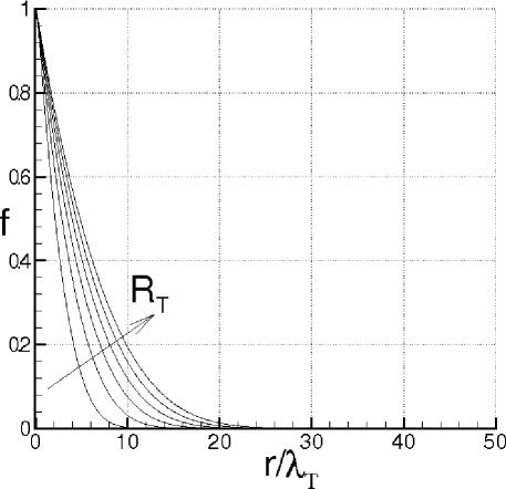
Figure 1: Longitudinal correlation function for different Taylor-Scale Reynolds numbers.

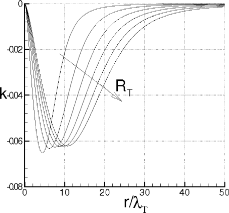
Figure 2: Longitudinal triple correlation function for different Taylor-Scale Reynolds numbers.

Therefore, the boundary problem represented by Eqs. (156), (139), is replaced by the following initial condition problem

$$\begin{array}[]{l@{\hspace{+0.cm}}l}\displaystyle\frac{df}{d\hat{r}}=F\\ \\ \displaystyle\frac{dF}{d\hat{r}}=-\frac{5f\hat{r}}{\sqrt{2(1-f)}}-\left(\frac{1}{2}\sqrt{\frac{1-f}{2}}R_{T}+\frac{4}{\hat{r}}\right)F\end{array}$$ (161)

whose initial condition is

$$\displaystyle f(0)=1,\ F(0)=0$$ (162)

8 Results and Discussion

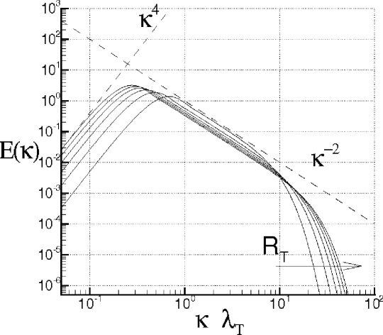
Figure 3: Steady Energy Spectrum for different Taylor-Scale Reynolds numbers.

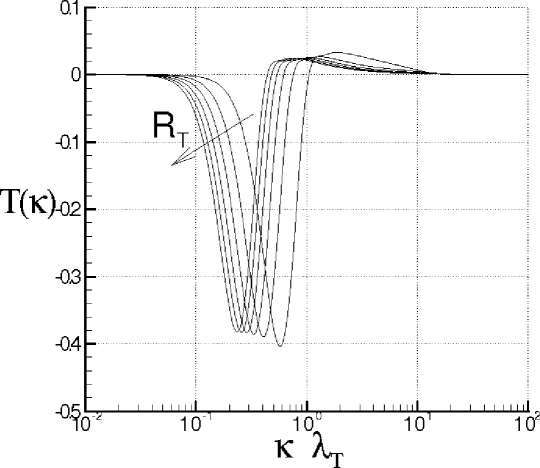
Figure 4: Steady ”Transfer function $T(\kappa)$” for several Taylor-Scale Reynolds numbers.

It is worth to remark that Eq. (156) is quite similar to the equation obtained by de Divitiis (2011) in the case of self-similar isotropic turbulence.

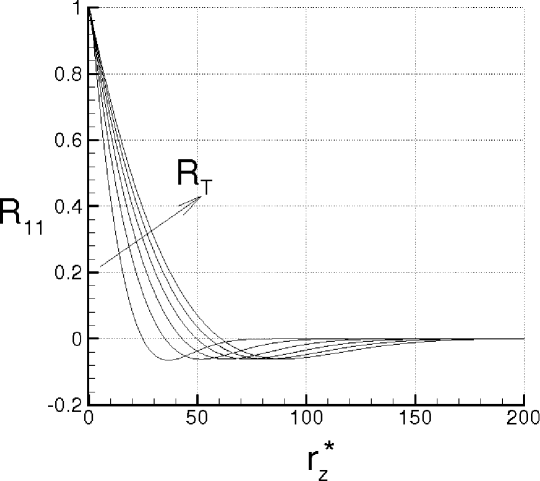
Figure 5: Spanwise correlation function of the streamwise component of velocity for several Taylor-Scale Reynolds numbers.

There, the equation was

$$\begin{array}[]{l@{\hspace{-0.cm}}l}\displaystyle\sqrt{\frac{1-f}{2}}\ \frac{df}{d\hat{r}}+\displaystyle\frac{2}{R_{T}}\left(\frac{d^{2}f}{d\hat{r}^{2}}+\displaystyle\frac{4}{\hat{r}}\frac{df}{d\hat{r}}\right)+\frac{10}{R_{T}}f=0\end{array}$$ (164)

where again, ${d^{2}f(0)}/{d\hat{r}^{2}}=-1$ and the boundary conditions are expressed by Eq. (157). Equation (156) differs from Eq. (164) by the presence of the last term, that, into Eq. (164), arises from $\partial u^{2}/\partial t$ under the self-similarity hypothesis. de Divitiis (2011) shows that $f-1\approx r^{2/3}$, where $2/R_{T}\left(d^{2}f/d\hat{r}^{2}+4/\hat{r}df/d\hat{r}\right)$ is negligible with respect to the other terms (see Eq. (164)). This determines that $E(\kappa)\approx\kappa^{-5/3}$ in the inertial subrange and that the scaling law $\langle(\Delta u_{r})^{n}\rangle\approx r^{\zeta_{n}}$ is satisfied for $\zeta_{n}\simeq n/3$. Here, the presence of third term of Eq. (156) modifies the correlation function, resulting $f-1\approx r$ and this implies that $E(\kappa)\approx\kappa^{-2}$ in the inertial subrange and that $\zeta_{n}\simeq n/2$.

Figure 6: Skewness of $\Delta u_{r}$ at different Taylor-Scale Reynolds numbers.

Figure 7: Flatness of $\Delta u_{r}$ at different Taylor-Scale Reynolds numbers.

To study in detail the energy spectrum, several numerical solutions of Eqs. (161) are calculated for different values of $R_{T}$ by means of the fourth-order Runge-Kutta method. The step of integration is chosen on the basis of the behavior of Eqs. (161) at the small scales when $r\rightarrow\infty$. There, $d^{2}f/d\hat{r}^{2}$ is about equal to $K$

$$\begin{array}[]{l@{\hspace{-0.cm}}l}\displaystyle\frac{d^{2}f}{d\hat{r}^{2}}\approx\displaystyle-\frac{R_{T}}{2\sqrt{2}}\frac{df}{d\hat{r}}\end{array}$$ (166)

This equation suggests that $\Delta\hat{r}=\sqrt{2}/R$ can be an adequate step of integration (Hildebrand (1987)) for the accuracy of the numerical solutions of Eq. (161).

As in de Divitiis (2011), the cases here studied correspond to $R_{T}$ = $100$, $200$, $300$, $400$, $500$ and $600$.

Figures 1 and 2 show double and triple longitudinal correlation functions. Due to the mechanism of energy cascade expressed by $K$ ( see Eq. (131)), the tail of $f$ rises with $R_{T}$ in agreement with Eq. (135) and this determines that, for an assigned value of $\lambda_{T}$, all the integral scales of $f$ increase with $R_{T}$. Comparing these results with the corresponding data of de Divitiis (2011), we found that, the integral scales here calculated are about one-sixth those obtained in the case of homogeneous isotropic turbulence. This means that $\nabla_{\bf x}{\bf U}$ contrasts the mechanism of the energy cascade, making this mechanism more limited in scales.

According to Eq. (131), $k$ decays more slowly than $f$ and its characteristic scales increase with $R_{T}$ as prescribed by Eq. (161). The maximum of $|k|$ is about 0.06 and this is in very good agreement with the numerous data of the literature (see Batchelor (1953) and Refs. therein). Again, the scales of variation of $k$ are almost one-sixth those calculated in de Divitiis (2011).

Figures 3 and 4 show $E(\kappa)$ and $T(\kappa)$ calculated with Eq. (153). Because of the fluid incompressibility (see Eq. (136)), $E(\kappa)\approx\kappa^{4}$ near the origin, whereas $E(\kappa)\approx\kappa^{-2}$ in the inertial subrange in contrast with Kolmogorov law $\kappa^{-5/3}$. This disagreement, caused by $\nabla_{\bf x}{\bf U}$, makes the mechanism of energy cascade weaker with respect to the isotropic turbulence, in agreement with the previous observation, determining a higher absolute slope of $E(\kappa)$ in the inertial range. For what concerns $T(\kappa)$, as $K$ does not modify the fluid kinetic energy, $\int_{0}^{\infty}T(\kappa)d\kappa=$ 0 (see Fig. 4).

Note that these cases can represent homogeneous turbulent flows with uniform steady shear rate

$$\nabla_{\bf x}{\bf U}=\frac{\partial U}{\partial y}\left[\begin{array}[]{ccc}\displaystyle 0&1&0\\ \\ \displaystyle 0&0&0\\ \\ \displaystyle 0&0&0\end{array}\right]$$ (172)

where $x$ and $z$ are streamwise and spanwise coordinates, respectively. In this situation we expect that $\nabla_{\bf x}{\bf U}$ leads to the development of coherent structures, similar to streaks, caused by the stretching of the vortex lines along $x$ (Lee, Kim & Moin (1990)). This influences the spanwise correlation function of the streamwise velocity $R_{11}(r_{z})$ which is here calculated through Eq. (85), once $f$ is known. The results, shown in Fig. 5, give $R_{11}(r_{z})$ in terms of the dimensionless coordinate $r_{z}^{*}=r_{z}/(\nu/\sqrt{S})^{1/2}$ and show that $R_{11}(r_{z})$ intersects the horizontal axis and remains negative for $r_{z}\rightarrow\infty$. These negative values imply a wide distribution of spacings between the different streaky structures, whose mean value depends on $R_{T}$ (Lee, Kim & Moin (1990)). From the figure, this average distance results to be about $70\div 150$ in units of viscous scale $(\nu/\sqrt{S})^{1/2}$, comparable with the results of Ref. (Lee, Kim & Moin (1990)).

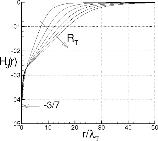
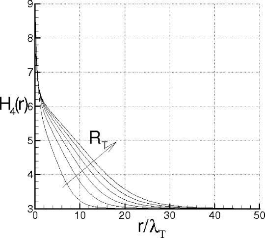
Figures 6 and 7 illustrate skewness and flatness of $\Delta u_{r}$ for the same values of $R_{T}$. The skewness $H_{3}$ is first calculated with Eq. (175) and the flatness $H_{4}$ has been thereafter determined using Eq. (183).

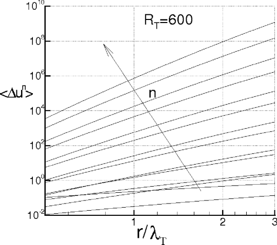
Figure 8: Statistical moments of $\Delta u_{r}$ in terms of the separation distance, for $R_{T}$=600.

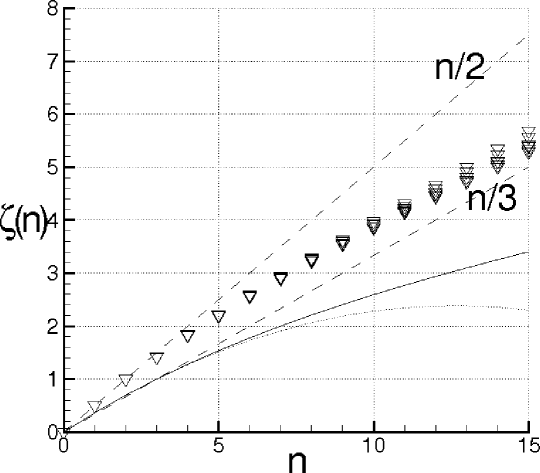
Figure 9: Scaling exponents of $\Delta u_{r}$ for several $R_{T}$. Solid symbols are for the present data. Dashed line is for Kolmogorov (1941). Dotted line is for Kolmogorov (1962). Continuous line is for She-Leveque (1994)

Although $H_{3}(0)$ does not depend upon the Reynolds number (de Divitiis (2010)) (see Appendix), for $r>\lambda_{T}$, $H_{3}(\hat{r})$ rises with $R_{T}$ and goes to zero for $r\rightarrow\infty$. The constancy of $H_{3}(0)$ and the quadratic terms of Eq. (177) cause that the intermittency of $\Delta u_{r}$ increases with $R_{T}$, whereas the spatial variations of $H_{3}$ and $H_{4}$ are the result of $f(r)$, $k(r)$ and of Eq. (177), thus also the scales of variation of skewness and flatness are significantly smaller in comparison with those of the isotropic turbulence. The quantity $H_{4}-3$ is significantly greater than zero for $r=0$ and tends to zero as $r\rightarrow\infty$ more rapidly than $H_{3}$.

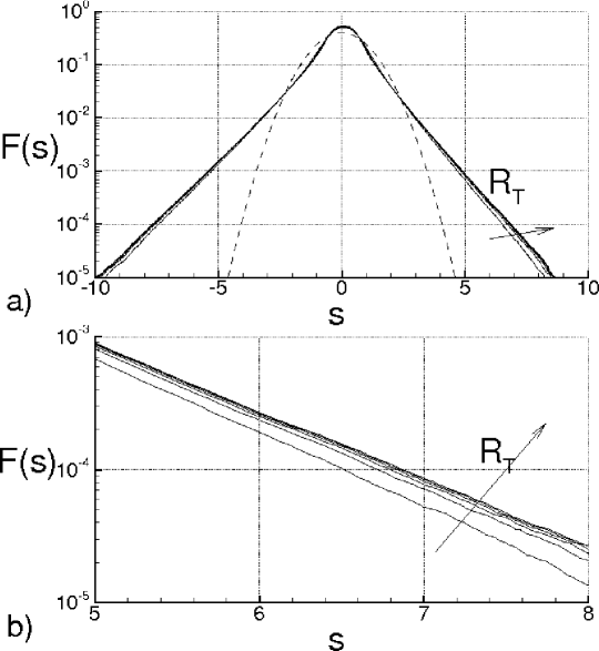
Figure 10: Probability distribution functions of the longitudinal velocity derivative for the different Taylor-Scale Reynolds numbers

The spatial structure of $\Delta u_{r}$ is studied with the analysis reported in the Appendix (de Divitiis (2010)), using the previous results. The statistical moments of $\Delta u_{r}(r)$ are expressed in function of $r$ through different scaling exponents $\zeta_{n}$

$$\left\langle(\Delta u_{r})^{n}\right\rangle=A_{n}r^{\zeta_{n}}$$ (173)

Table 1: Scaling exponents of the longitudinal velocity difference for several Taylor-Scale Reynolds number.

$R_{T}$	100	200	300	400	500	600
$\zeta_{1}$	0.49	0.50	0.50	0.50	0.50	0.50
$\zeta_{2}$	1.00	1.00	1.00	1.00	1.00	1.00
$\zeta_{3}$	1.42	1.41	1.41	1.41	1.41	1.41
$\zeta_{4}$	1.84	1.83	1.82	1.82	1.83	1.83
$\zeta_{5}$	2.22	2.19	2.19	2.19	2.20	2.20
$\zeta_{6}$	2.59	2.56	2.56	2.56	2.57	2.58
$\zeta_{7}$	2.94	2.89	2.90	2.90	2.91	2.93
$\zeta_{8}$	3.28	3.23	3.23	3.24	3.26	3.29
$\zeta_{9}$	3.60	3.54	3.55	3.56	3.59	3.63
$\zeta_{10}$	3.92	3.85	3.87	3.88	3.93	3.98
$\zeta_{11}$	4.22	4.15	4.17	4.19	4.26	4.32
$\zeta_{12}$	4.53	4.44	4.47	4.51	4.58	4.66
$\zeta_{13}$	4.81	4.72	4.75	4.81	4.91	5.00
$\zeta_{14}$	5.10	5.00	5.04	5.11	5.24	5.35
$\zeta_{15}$	5.39	5.28	5.33	5.42	5.56	5.69

In order to calculate $\zeta_{n}$, $\langle\Delta u_{r}^{n}\rangle$ are first calculated in function of $\hat{r}$, through Eqs. (183) (see for instance Fig. 8). The scaling exponents are identified through a best fitting procedure, in the intervals ($\hat{r}_{1},\hat{r}_{2}$), where the endpoints $\hat{r}_{1}$ and $\hat{r}_{2}$ have to be determined. The calculation of $\zeta_{n}$ and $A_{n}$ is carried out through a minimum square method which, for each statistical moment, is applied to the following optimization problem

$$\displaystyle J_{n}(\zeta_{n},A_{n})\equiv\int_{\hat{r}_{1}}^{\hat{r}_{2}}\displaystyle(\langle(\Delta u_{r})^{n}\rangle-A_{n}r^{\zeta_{n}})^{2}dr=\mbox{min},\ n=1,2,...$$ (174)

where $\langle(\Delta u_{r})^{n}\rangle$ are calculated with Eqs. (183), $\hat{r}_{1}$ is assumed to be equal to $0.1$, whereas $\hat{r}_{2}$ is taken in such a way that $\zeta_{2}$ = 1 for all the values of $R_{T}$. The so obtained scaling exponents, shown in Table 1, are compared in Fig. 9 (solid symbols) with those of the Kolmogorov theories K41 (Kolmogorov (1941)) (dashed line) and K62 (Kolmogorov (1962)) (dotted line), and with the exponents calculated by She-Leveque (1994) (continuous curve). We found that, near the origin $\zeta_{n}\simeq n/2$ instead of the expected law $\zeta_{n}\simeq n/3$, whereas for $n>4$, $\zeta_{n}$ behaves like a multiscaling exponent. This is in agreement with the experimental results of Baroud et al (2002), where the turbulence is produced in a cylindrical rotating tank. The multiscaling behavior is the consequence of the combined effect of the quadratic terms of Eq. (177) and of the mechanism of the energy cascade expressed by $K$ through Eqs. (131).

Next, to analyse the statistics of $\partial u_{r}/\partial{\hat{r}}$, the distribution functions of $\partial u_{r}/\partial{\hat{r}}$ are calculated using Eqs. (196) and (177). These are obtained with sequences of the variables $\xi$, $\eta$ and $\zeta$ generated by gaussian random numbers generators. The distribution functions are then calculated through the statistical elaboration of these data and Eq. (177). The results are shown in Fig. 10a and 10b in terms of the dimensionless abscissa

$$\displaystyle s=\frac{\partial u_{r}/\partial{\hat{r}}}{\langle\left(\partial u_{r}/\partial{\hat{r}}\right)^{2}\rangle^{1/2}}$$

where the dashed curve represents the gaussian PDF. These distribution functions are normalized, in order that their standard deviations are equal to the unity. In particular, Fig. 10b shows the enlarged region of Fig. 10a, where $5<s<8$. The tails of the PDFs change with $R_{T}$ in such a way that the intermittency rises with $R_{T}$ according to Eq. (177).

9 Conclusions

The equation of the steady spherical correlation function is obtained in case of homogeneous turbulence in the presence of an uniform average velocity gradient, and an expression of the velocity correlation tensor in terms of this gradient is derived. When $r=0$, this tensor recovers the Boussinesq closure of the Reynolds stress. The solutions of this equation, calculated with the closure based on a specific Lyapunov theory previously proposed, allows to determine the statistics of $\Delta u_{r}$. In particular:

• The energy spectrum, satisfying the continuity equation, follows the law $\kappa^{-2}$ in the inertial subrange whose size increases with the Reynolds number. This contrasts with the Kolmogorov law and represents a more tenuous mechanism of the energy cascade. Accordingly, the scaling exponents of the moments of velocity difference vary according to $\zeta_{n}\approx n/2$ instead of $\zeta_{n}\approx n/3$, and for $n>4$, these exponents exhibit multiscaling behavior.

• The effect of the average velocity gradient, going against the mechanism of energy cascade, makes the integral scales of $f$ and the scales of variations of $k$, significantly smaller than those calculated for the isotropic turbulence.

• In case of uniform shear rate, the spanwise correlation function of the streamwise velocity component, exhibits the typical shape caused by the streaky coherent structures due to the vortex stretching.

These results, which represent a further application of the analysis presented in de Divitiis (2010) and de Divitiis (2011), are comparable with the direct simulations of Lee, Kim & Moin (1990) and are in agreement with the theoretical arguments of Gordienko et al (2001) and with the experiments presented in Baroud et al (2002).

10 Appendix: Statistics of velocity difference

In this appendix, we recall the main results of de Divitiis (2010). For sake of simplicity, we only consider the statistics of the longitudinal velocity difference $\Delta u_{r}$ associated to $R_{ik0}$ (or $f$) and to Eq. (138). This approximation allows to calculate all the dimensionless statistical moments of $\Delta u_{r}$ once known the skewness $H_{3}(r)$. This latter is calculated in terms of $f$ and $k$ (Batchelor (1953))

$$\displaystyle H_{3}(r)=\frac{\left\langle(\Delta u_{r})^{3}\right\rangle}{\left\langle(\Delta u_{r})^{2}\right\rangle^{3/2}}=\frac{6k(r)}{\left(2(1-f(r))\right)^{3/2}}$$ (175)

hence, $H_{3}(0)=-3/7$ does not depend upon the Reynolds number (de Divitiis (2010)), and the higher order moments are consequentely determined, taking into account that $\Delta u_{r}$ is analytically expressed as

$$\begin{array}[]{l@{\hspace{+0.2cm}}l}\displaystyle\frac{\Delta{u}_{r}}{\sqrt{\langle(\Delta{u}_{r})^{2}}\rangle}=\displaystyle\frac{{\xi}+\psi\left(\chi({\eta}^{2}-1)-\displaystyle({\zeta}^{2}-1)\right)}{\sqrt{1+2\psi^{2}\left(1+\chi^{2}\right)}}\hfil\hskip 5.69046pt\end{array}$$ (177)

Equation (177), arising from statistical considerations about the Fourier-transformed Navier-Stokes equations, expresses the internal structure of the fully developed turbulence, where $\xi$, ${\eta}$ and $\zeta$ are independent centered random variables, each distributed following the gaussian distribution functions $p(\xi)$, $p(\eta)$ and $p(\zeta)$ whose standard deviation is equal to the unity. The moments of $\Delta{u}_{r}$ are easily calculated from Eq. (177)

$$\begin{array}[]{l@{\hspace{+0.2cm}}l}\displaystyle H_{n}\equiv\frac{\left\langle(\Delta u_{r})^{n}\right\rangle}{\left\langle(\Delta u_{r})^{2}\right\rangle^{n/2}}=\displaystyle\frac{1}{(1+2\psi^{2}\left(1+\chi^{2}\right))^{n/2}}\hfil\hskip 5.69046pt\\ \hfil\hskip 5.69046pt\\ \displaystyle\sum_{k=0}^{n}\left(\begin{array}[]{c}n\\ k\end{array}\right)\psi^{k}\langle\xi^{n-k}\rangle\langle(\chi(\eta^{2}-1)-(\zeta^{2}-1))^{k}\rangle\hfil\hskip 5.69046pt\end{array}$$ (183)

where

$$\begin{array}[]{l@{\hspace{+0.2cm}}l}\displaystyle\langle(\chi(\eta^{2}-1)-(\zeta^{2}-1))^{k}\rangle=\displaystyle\sum_{i=0}^{k}\left(\begin{array}[]{c}k\\ i\end{array}\right)(-\chi)^{i}\langle(\zeta^{2}-1)^{i}\rangle\langle(\eta^{2}-1)^{k-i}\rangle,\hfil\hskip 5.69046pt\\ \hfil\hskip 5.69046pt\\ \displaystyle\langle(\eta^{2}-1)^{i}\rangle=\sum_{l=0}^{i}\left(\begin{array}[]{c}i\\ l\end{array}\right)(-1)^{l}\langle\eta^{2(i-l)}\rangle\hfil\hskip 5.69046pt\end{array}$$ (191)

In particular, $H_{3}$, related to the energy cascade, is

$$\displaystyle H_{3}=\frac{8\psi^{3}\left(\chi^{3}-1\right)}{\left(1+2\psi^{2}\left(1+\chi^{2}\right)\right)^{3/2}}$$ (192)

and $\psi$ is a function of $r$ and of the Reynolds number de Divitiis (2010)

$$\psi({\bf r},R_{T})=\sqrt{\frac{R_{T}}{15\sqrt{15}}}\ \hat{\psi}(r)$$ (193)

being $\hat{\psi}(r)$ determined through Eq. (192) as soon as $H_{3}(r)$ is known. The parameter $\chi$ is also a function of $R_{T}$ and is implicitly calculated putting $r=0$ into Eq. (192)

$$\frac{8{\psi_{0}}^{3}\left(1-\chi^{3}\right)}{\left(1+2{\psi_{0}}^{2}\left(1+\chi^{2}\right)\right)^{3/2}}=\frac{3}{7}$$ (194)

where ${\psi_{0}}=\psi(R_{T},0)$ and $\hat{\psi_{0}}=1.075$ de Divitiis (2010).

The PDF of $\Delta u_{r}$ can be formally expressed through the gaussian PDFs $p(\xi)$, $p(\eta)$ and $p(\zeta)$, using the Frobenius-Perron equation (Nicolis (1995))

$$\begin{array}[]{l@{\hspace{+0.3cm}}l}F(\Delta{u^{\prime}}_{r})=\displaystyle\int_{\xi}\int_{\eta}\int_{\zeta}p(\xi)p(\eta)p(\zeta)\ \delta\left(\Delta u_{r}-\Delta{u^{\prime}}_{r}\right)\ d\xi d\eta d\zeta\hfil\hskip 8.5359pt\end{array}$$ (196)

References

• Brissaud et al (1973) Brissaud, A., Frisch, U., Leorat, J., Lessieur, M., and Mazure, A., Helicity cascades in fully developed isotropic turbulence, Phys. Fluids, 16, 1366–1367, 1973.
• Moffat (1978) Moffat, H. K., Magnetic Field Generation in Electrically Conducting Fluids, Cambridge Univ. Press, Cambridge, 1978..
• Gordienko et al (2001) Gordienko S. N. and Moiseev S. S., Turbulence: mechanics and structure of anomalous scaling, Nonlin. Processes Geophys., 8, 197-200, 2001.
• Baroud et al (2002) Baroud C. N., Plapp B. B., She Z. S., and Swinney H. L., Anomalous Self-Similarity in a Turbulent Rapidly Rotating Fluid, Phys. Rev. Lett. 88, 114501, 2002.
• Lee, Kim & Moin (1990) Lee M. J., Kim J., and Moin P., Structure of turbulence at high shear rate, J. Fluid Mech., 216, 561-583, 1990.
• de Divitiis (2010) de Divitiis N., Lyapunov Analysis for Fully Developed Homogeneous Isotropic Turbulence, Theoretical and Computational Fluid Dynamics, DOI: 10.1007/s00162-010-0211-9.
• de Divitiis (2011) de Divitiis N., Self-Similarity in Fully Developed Homogeneous Isotropic Turbulence Using the Lyapunov Analysis, Theoretical and Computational Fluid Dynamics, DOI: 10.1007/s00162-010-0213-7.
• Kármán-Howarth (1938) von Kármán, T. & Howarth, L., On the Statistical Theory of Isotropic Turbulence., Proc. Roy. Soc. A, 164, 14, 192, 1938.
• Batchelor (1953) Batchelor, G. K., The Theory of Homogeneous Turbulence. Cambridge University Press, Cambridge, 1953.
• Nicolis (1995) Nicolis, G., Introduction to nonlinear science, Cambridge University Press, 1995.
• Batchelor (1967) Batchelor, G. K., An introduction to fluid dynamics. Cambridge University Press, Cambridge, 1967.
• Hildebrand (1987) Hildebrand, F. B., Introduction to Numerical Analysis, Dover Publications, 1987.
• Kolmogorov (1941) Kolmogorov, A. N., Dissipation of Energy in Locally Isotropic Turbulence. Dokl. Akad. Nauk CCCP 32, 1, 19–21, 1941.
• Kolmogorov (1962) Kolmogorov, A. N., Refinement of Previous Hypothesis Concerning the Local Structure of Turbulence in a Viscous Incompressible Fluid at High Reynolds Number, J. Fluid Mech. 12, 82–85, 1962.
• She-Leveque (1994) She, Z. S. and Leveque, E., Universal scaling laws in fully developed turbulence, Phys. Rev. Lett. 72, 336, 1994.