Wronskian Solution for AdS/CFT Y-system

Abstract:

Using the discrete Hirota integrability we find the general solution of the full quantum Y-system for the spectrum of anomalous dimensions of operators in the planar AdS₅/CFT₄ correspondence in terms of Wronskian-like determinants parameterized by a finite number of Baxter’s Q-functions. We consider it as a useful step towards the construction of a finite system of non-linear integral equations (FiNLIE) for the full spectrum. The explicit asymptotic form of all the Q-functions for the large size operators is presented. We establish the symmetries and the analyticity properties of the asymptotic Q-functions and discuss their possible generalization to any finite size operators.

1 Introduction

The Y-system for the full spectrum of energies/dimensions in the planar AdS₅/CFT₄ system conjectured in [1] has passed a few important tests. It was re-derived and better understood within the TBA approach [2, 3, 4] and successfully tested in the weak coupling by comparison with the perturbative expansion in N=4 SYM theory up to 4-5 loops [5, 6, 7, 8, 9]. Remarkably, the very same Y-system was shown to be responsible for the spectrum of $\beta$-deformed $N=1$ case in [10] where the perturbative results [6, 11] were reproduced up to $11$ loops . At strong coupling the Y-system perfectly reproduces the results of quasi-classical quantization of highly excited states of the superstring in $\mathfrak{sl}_{2}$ sector, in the regime where there is no way to ignore the finite size effects [12], demonstrating that the formidable wrapping problem finds its successful resolution within the Y-system. Furthermore, some of these results were extended to the generic finite-gap string state in [13] and to the ABJM model in [14].

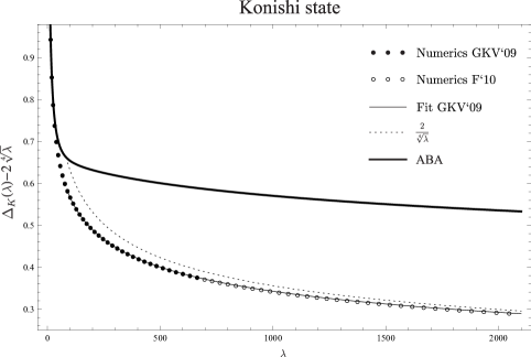
Figure 1: Numerical results of solution of the AdS/CFT Y-system (in integral, TBA form) for Konishi dimension as a function of ‘t Hooft coupling $\lambda$ (from [15] and [16]).

The numerical calculation of the Konishi dimension from the Y-system, combined with the TBA approach in [15], has provided the data covering a range of values of the ‘t Hooft coupling enough to confirm the leading strong coupling asymptotics $2\lambda^{1/4}$ obtained on the string side of the duality [17] and to predict, with a reasonable accuracy, the next, subleading correction as being $1.99\cdot\lambda^{-1/4}$. A more extensive numerical study recently done in [16] allowed to extend the range of the interval of ‘t Hooft couplings in the strong coupling regime by more than $3$ times. This new data from [16] perfectly confirms old results: the new points follow the fitting curve from [15], within the accuracy margins (see Fig.1).

By now it is fair to say that the Y-system is the correct framework to study the spectrum of this important duality. However there are still many open problems. The main problem which has been preventing us from applying the Y-system to more complicated states is to convert it into a system of integral equations suitable for numerical/analytical study at intermediate couplings. This problem was only solved for some simple states like the Konishi state. It is important to understand the properties of a general solution of Y-system describing the physical states of AdS/CFT correspondence.

The AdS/CFT Y-system is an infinite set of functional equations on the functions of a spectral parameter, related to the Hirota bi-linear difference equation (T-system) well known in quantum integrability. It differs from the Y-systems for the previously known quantum integrable models (1D spin chains, sigma-models etc.) by the specific, so called $\mathbb{T}$-hook boundary conditions in the representation space (w.r.t. the discrete indices living on a 2D lattice $(a,s)\in\mathbb{Z}\times\mathbb{Z}$) and complicated analyticity properties w.r.t. the spectral parameter.

On the other hand, it is known from our experience with some relativistic sigma models and spin chains that the same quantum systems described at a finite volume by a Y-system may obey a rather different, finite set of non-linear integral equations (which we will abbreviate here as FiNLIE). The first example of such equations, called DdV equations, were given by Destri and deVega for the Thirring model [18] followed by a considerable activity in this direction. A new approach for the search of such FiNLIE for the integrable sigma-models based on the integrable Hirota dynamics of the Y-system, together with a few simple assumptions on its analyticity structure, was proposed in [19] and developed in [20]. It relies on the fact that the Y-system, or the underlying T-system, can be solved in terms of a finite number of ${\mathsf{Q}}$-functions, analogs of those introduced by Baxter for the XXZ chain. The T-functions can be represented in terms of finite determinants (Wronskians) of those ${\mathsf{Q}}$-functions and, knowing the analyticity properties of ${\mathsf{Q}}$’s, one can then write a FiNLIE solving the finite size problem.

Such a FiNLIE would be a very welcome progress for the study of the spectrum of AdS₅/CFT₄ system. It would provide us not only with a more efficient analytic and numerical tool for the study of this complex model but also most probably give some insight into the structure of this duality. However, due to the complexity of the $\mathbb{T}$-hook boundary conditions and of the analyticity properties of Y-functions, this FiNLIE remains unknown. We propose in this paper an important, in our opinion, step towards the derivation of such equations by writing a general Wronskian-type solution of the corresponding T-system for the $\mathbb{T}$-hook boundary conditions. This solution will be a natural generalization of our explicit general solution, found by three of the current authors [13] for a simplified T-system, relevant to the quasiclassical limit of the string sigma-model, in terms of characters of specific infinite-dimensional representations of $U(2,2|4)$, parameterized by 8 eigenvalues of an arbitrary group element. We will also demonstrate this construction in the asymptotic, large size limit (of long SYM operators) when the asymptotic Bethe ansatz (ABA) [22, 23] is applicable. We will also discuss the analyticity and symmetry properties of these ${\mathsf{Q}}$-functions. The relation of the character solution to the quasi-classical limit of the superstring on the $AdS_{5}\times S^{5}$ background discussed in [13] will serve as an important source of inspiration for that.

The T-system first appeared in the context of the quantum integrable systems for the $gl(2)$ algebra in [24], and generalized to $gl(N)$ in [25]. Wronskian determinant solutions of T-system were introduced in [26] for $N=2$ and in [27] for any $N$, where the finite dimensional representations of $gl(N)$ symmetry impose the boundary conditions in the semi-infinite strip of the width $N$ in the $(a,s)$-representation space. The Wronskian solutions were generalized to the supersymmetric $gl(M|N)$ algebras for the $T$-system with the $(M|N)$ fat hook boundary conditions for $(M,N)=(2,1)$ in [30, 31] and for any $(M,N)$ in [32]. On the way to constructing similar solutions for the $\mathbb{T}$-hook boundary conditions corresponding to the superconformal $PSU(2,2|4)$ symmetry of the model we will first remind the “classical” solution for the $U(2,2|4)$ characters [12, 13] and then discuss the most general form of the so called TQ-relations relating T- and ${\mathsf{Q}}$-functions (analogue of Baxter’s famous relation for the XXZ model), in the form of the so called generating functional [27], for finite [28, 29, 33], and even for the infinite-dimensional [34] representations of $gl(M|N)$, as well as the QQ-relations among the ${\mathsf{Q}}$-functions, especially efficient for the super-algebras [35, 33] (see also earlier papers [36, 29]). The Bäcklund solution of Hirota equation for the $gl(M)$ algebras [27] and $gl(M|N)$ super-algebras, for the fat hook boundary conditions in the representational $(a,s)$ space [33], was generalized to the case of a general $\mathbb{T}$-hook in [37]. The latter can be conveniently rewritten through the generating functional [34, 13] further used in this paper.

The Wronskian solution for the AdS/CFT Y-system which we are proposing in this paper summarizes in the most explicit and concise way all these developments. Its main advantage w.r.t. the previous solutions [37, 13] of the Y-system (and the associated T-system) in the $\mathbb{T}$-hook is its absolutely explicit form in terms of the Wronskian determinants of a finite number of Baxter’s Q-functions (7 independent Q-functions) which does not include any infinite sums or integral operators. We consider this Wronskian representation as a good starting point for trying to derive a FiNLIE system describing the spectrum of the planar AdS₅/CFT₄.

2 $Y$-system and $T$-system for the spectrum of AdS/CFT

In this section we will remind the Y-system for the spectrum of AdS₅/CFT₄, point out its symmetries and discuss its analytic properties.

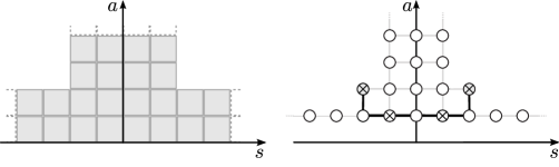
Figure 2: T-shaped “fat hook” ($\mathbb{T}$-hook) uniting two ${\rm SU}(2|2)$ fat hooks, see [1] for this $\mathbb{T}$-hook and its generalization [37].

The problem of the spectrum of the closed superstring sigma model on the $AdS_{5}\times S^{5}$ background, similarly to all known integrable sigma models on a space-time cylinder with the global $gl(M|N)$ type symmetry, can be reduced to the Y-system [1]

$$Y_{a,s}^{+}Y_{a,s}^{-}=\frac{(1+Y_{a,s+1})(1+Y_{a,s-1})}{(1+1/Y_{a+1,s})(1+1/Y_{a-1,s})}\,$$ (1)

where $Y_{a,s}$ are functions of the spectral parameter $u$, defined on the visible nodes of the two-dimensional integer $(a,s)$-lattice presented on the Fig.2(right). By the subscripts $f^{\pm}$ of any function $f(u)$ of $u$, we denote the shifts of the spectral parameter by $\pm\frac{i}{2}$: $f^{\pm}\equiv f(u\pm\frac{i}{2})$.

What distinguishes the Y-systems for various sigma models is: 1) the boundary conditions on the $a,s$ lattice which are mostly defined by the symmetry of the model 2) the analytic properties w.r.t. the spectral parameter $u$, only partially constrained by the symmetry and greatly depending on the physical properties of the model.

The Y-system for AdS/CFT, as any Y-system, is directly related to the so called T-system. Namely, defining

$$Y_{a,s}=\frac{T_{a,s+1}T_{a,s-1}}{T_{a+1,s}T_{a-1,s}}\;$$ (2)

we rewrite (1) in terms of the bilinear finite difference Hirota equation

$$T_{a,s}^{+}T_{a,s}^{-}=T_{a+1,s}T_{a-1,s}+T_{a,s+1}T_{a,s-1}\,.\\$$ (3)

For our string sigma model the boundary conditions on the $a,s$ lattice are constrained by the superconformal $PSU(2,2|4)$ symmetry [13] and impose that the T-functions, are nonzero only inside the so called ${\mathbb{T}}$-hook [1], i.e. only on the nodes of the visible part of the $(a,s)$-lattice of the Fig.2(left). The rest of the T-functions are zero:

$$T_{a,s}=0\qquad\text{for}\qquad a<0\cup(a>2\cap|s|>2)\;.$$ (4)

These boundary conditions for the functions $T_{a,s}$ agree with the above mentioned boundary conditions for the functions $Y_{a,s}$ of the Fig.2(right) if we take Y-functions to be zero on the vertical boundaries, and to be infinite on the horizontal boundaries on the Fig.2(left). Note that this leaves an ambiguity about the values at the corner nodes $Y_{2,\pm 2}$. A more careful analysis shows that equations for $Y_{2,\pm 2}$ are more complicated and cannot be written in a “local” functional form. The two missing equations (11) do not have the standard Y-system form and can be borrowed from the TBA approach [2]. However, we believe that all the functions $T_{a,s}$ satisfy the standard Hirota equation (3) [1]. In that sense, the T-system looks more universal, and in many cases more convenient than the Y-system.

Notice that the parameterization in terms of $T_{a,s}$ is not unique. The T-system is invariant under the gauge transformation:

$$T_{a,s}\to g_{1}^{[a+s]}g_{2}^{[a-s]}g_{3}^{[s-a]}g_{4}^{[-a-s]}T_{a,s}$$ (5)

and thus the T-functions are defined up to 4 arbitrary gauge functions $g_{a}(u)$. The physical quantities are computed in terms of the gauge invariant $Y$-functions.

The analytic structure of the AdS/CFT Y-system is inherited to a great extent from the dispersion relations for the elementary physical excitations – the magnons on the infinite spin chain representing a SYM operator, or its AdS dual on the string side. The dispersion relation between the energy and the momentum of such solitary excitations [38] is conveniently parameterized [39] by the so called Zhukovsky map $\frac{u}{g}=x+1/x$, where $g$ is related to the ‘t Hooft’s coupling $\lambda=g_{YM}N_{c}^{2}$ as $g=\frac{\sqrt{\lambda}}{4\pi}$:

$$p(u)=\frac{1}{i}\log\left(\frac{x^{+}(u)}{x^{-}(u)}\right)\;\;,\;\;{\epsilon}(u)=1+\frac{2ig}{x^{+}(u)}-\frac{2ig}{x^{-}(u)}\;.$$ (6)

The inverse map is double valued and we have to distinguish two branches – physical and mirror (related to the exchange of time and space coordinates on the world sheet cylinder [40, 41]):

$$\qquad x^{\rm ph}(u)=\frac{1}{2}\left(\frac{u}{g}+\sqrt{\frac{u}{g}-2}\;\sqrt{\frac{u}{g}+2}\right)\;,\qquad x^{\rm mir}(u)=\frac{1}{2}\left(\frac{u}{g}+i\sqrt{4-\frac{u^{2}}{g^{2}}}\right)\,.$$ (7)

In the physical branch, the finite cut, by definition, connects two branch points $u=\pm 2g$ whether as in the mirror branch the cut connecting them passes through the infinity.

The $u$-parameterization is distinguished by the fact that the fusion of elementary excitations into various bound states is especially simple in the complex $u$-plane: the rapidities of the constituents of a bound state are spaced by the integers of $i$. For example, the bound states for the energy carrying magnons mentioned above have the energy and momentum [42]

$$\exp p_{a}(u)={\cal F}_{a}\circ\exp p(u),\qquad\exp\epsilon_{a}(u)={\cal F}_{a}\circ\exp\epsilon(u)$$ (8)

where we defined the fusion operator

$${\cal F}_{a}\circ f(u)=\left\{\begin{array}[]{cl}\prod\limits_{j=-\frac{|a|-1}{2}}^{\frac{|a|-1}{2}}f(u+ij)&,\;\;a>0\\ 1&,\;\;a=0\\ \prod\limits_{j=-\frac{|a|-1}{2}}^{\frac{|a|-1}{2}}1/f(u+ij)&,\;\;a<0\end{array}\right.\;.$$ (9)

This gives for the dispersion relation of the bound states

$$p_{a}(u)=\frac{1}{i}\log\left(\frac{x^{[+a]}}{x^{[-a]}}\right),\qquad{\epsilon}_{a}(u)=a+\frac{2ig}{x^{[+a]}}-\frac{2ig}{x^{[-a]}}\;.$$ (10)

The Y-functions as functions of $u$ should inherit the multi-valuedness of the map (7). Most of our experience on their analyticity properties comes from the asymptotic Bethe ansatz (ABA) [22, 23] corresponding to the limit of very long operators $L\to\infty$ and from TBA equations for the excited states [3, 2, 4]. The ABA limit of Y-system found in [1] shows that the Y-functions have branch points at $u=\pm 2g+\frac{in}{2}$ for various $n$’s ($n\in{\mathbb{Z}}$). Similarly to the above definition of $x^{\rm mir}$ we define the “mirror” sheet of the $Y$-functions with the cuts going through infinity, parallel to the real axis. We can find from the study of the ABA limit (see the section 5) that $\left.Y_{1,s}\right|_{s\geqslant 2}$ has 4 branch cuts at ${\rm Im}\;u=\tfrac{\pm s\pm 1}{2}$, while $\left.Y_{a,\pm 1}\right|_{a\geqslant 2}$ has 4 branch cuts at ${\rm Im}\;u=\tfrac{\pm a\pm 1}{2}$, and $Y_{1,\pm 1},\;Y_{2,\pm 2}$ have 3 cuts at ${\rm Im}\;u=0,\pm 1$. At finite size other cuts can appear, but we expect the following analyticity conditions to hold anyway [43]:

1. $Y_{1,\pm s}$ have no branch cuts inside the strip $-\tfrac{|s|-1}{2}<{\rm Im}\;u<\tfrac{|s|-1}{2}$;

2. $Y_{a,\pm 1}$ have no branch cuts inside the strip $-\tfrac{a-1}{2}<{\rm Im}\;u<\tfrac{a-1}{2}$;

3. $Y_{a,0}$ have no branch cuts inside the strip $-\tfrac{a}{2}<{\rm Im}\;u<\tfrac{a}{2}$;

4. $Y_{1,\pm 1},\;Y_{2,\pm 2}$ have a cut on the real axes such that

   $$Y_{1,\pm 1}(u+i0)Y_{2,\pm 2}(u-i0)=1\,,\qquad u\in(-\infty,-2g]\cup[2g,\infty);$$ (11)

5. $Y_{a,s}$ obtained from the generating functional should be real functions in “mirror” kinematics.

The $Y$-system should be satisfied for the mirror branch of $Y_{a,s}$ described above (i.e. for the cuts chosen to go through infinity). We also define the “physical” branch of $Y_{1,0}$ as an analytic continuation through the first cut above the real axis and then back to the real axis (as proposed in [15]), and denote the continued function as $Y^{\rm ph}_{1,0}$. These properties are very similar to the ones used in [19] to convert the $su(2)$ principal chiral filed theory Y-system into the corresponding FiNLIE.

Once the appropriate solution of the Y-system for a given physical state of the $\linebreak[1]\mathrm{AdS}_{5}/\mathrm{CFT}_{4}$ system is found its energy is given by the following formula

$$E=\sum_{j}\epsilon^{{\rm ph}}_{1}(u_{4,j})+\sum_{a=1}^{\infty}\int_{-\infty}^{\infty}\frac{du}{2\pi i}\,\,\frac{\partial\epsilon^{{\rm mir}}_{a}}{\partial u}\log\left(1+Y_{a,0}(u)\right)\;,$$ (12)

where we also have to impose the Bethe ansatz equation for the Bethe roots (the rapidities of physical excitations) [2, 15]

$$Y^{\rm ph}_{1,0}(u_{4,j})=-1\,.$$ (13)

the exact Bethe equations for the auxiliary roots should come from the condition of pole cancellation.

In the subsequent sections we first recall the solution of the $Y$-system in the classical large $\lambda$ limit given in terms of the characters and then describe our construction for the general quantum solution.

3 $SU(2,2|4)$ character solution of the Y-system and classical limit

In the classical limit when $\lambda$ is large the shifts by $\pm i/2$ in the (3) become irrelevant (see [12] for more details) and the functional $T$-system reduces to an algebraic set of equations called in the mathematical literature the $Q$-system:

$$\left(T_{a,s}\right)^{2}=T_{a+1,s}T_{a-1,s}+T_{a,s+1}T_{a,s-1}\,.$$ (14)

In the paper [13] three of the current authors clarified the group theoretical meaning of the AdS/CFT $Y$-system, its relation to the characters of irreducible representations of the $SU(2,2|4)$ symmetry, related to the superconformal $PSU(2,2|4)$ symmetry of the model, and their relation to the classical limit, extending some of the results of [12] to all sectors. We will briefly remind in this subsection the basic results concerning the explicit construction of the $SU(2,2|4)$ characters for the unitary representations, in terms of finite determinants, in full similarity to the 1-st Weyl formula known for the compact representations of $GL(N)$. In the next chapter we will show how to generalize these formulas to the quantum solution of the T-system (3), and to find the general explicit solution of the underlying $Y$-system and $T$-system in terms of finite determinants, called Wronskians, parameterized by a finite number of Baxter’s ${\mathsf{Q}}$-functions. We hope to apply these results in the future for the construction of a finite system of non-linear integral equations (FiNLIE) describing the full spectrum of the planar AdS${}_{5}/$CFT₄.

3.1 The character solution of the simplified AdS/CFT Y-system in $\mathbb{T}$-hook

The generating function of $U(2,2|4)$ characters of “symmetric” representations can be represented as

$$w_{4|4}(t;h)=\frac{(1-y_{{\hat{1}}}t)(1-y_{{\hat{2}}}t)}{(1-x_{{{1}}}t)(1-x_{{{2}}}t)}\times\frac{(1-y_{{\hat{3}}}t)(1-y_{{\hat{4}}}t)}{(1-x_{{{3}}}t)(1-x_{{{4}}}t)}$$ (15)

where $(x_{{1}},\dots,x_{{4}}|y_{\hat{1}},\dots,y_{\hat{4}})$ are the eigenvalues of a group element $h\in U(2,2|4)$. Here and below we use the hats over indexes to indicate their “fermionic” grading, as opposed to the “bosonic” grading of the rest of indices.

The first and the second factors in the r.h.s. may be attributed to the right and left $U(2|2)_{R,L}$ subgroups. The characters of “symmetric” representations are generated by

$$T_{1,s}^{(4|4)}[h]=\oint_{C}\frac{dt\,\,w_{4|4}(t;h)}{2\pi i}t^{-s-1}\;,$$ (16)

where the integration contour $C$ encircle $t=0$ together with the poles $\frac{1}{x_{{3}}},\frac{1}{x_{{4}}}$ corresponding to the subgroup $U(2|2)_{L}$, leaving outside the poles $\frac{1}{x_{{1}}},\frac{1}{x_{{2}}}\,$ corresponding to the first subgroup $U(2|2)_{R}$. Note that $s$ can here be positive as well as negative: $-\infty<s<\infty$ and the corresponding irreps, first constructed in [44, 45], are infinite-dimensional: $T_{1,s}^{(4|4)}[h]$ are not polynomials of $x_{i},y_{\hat{\jmath}}$ anymore, unlike the compact representations of $U(M|N)$. The rest of the $T_{a,s}(h)$ can be restored by means of the Jacobi-Trudi type formula:

$$T_{a,s}=\det_{1\leqslant i,j\leqslant a}\,T_{1,s+i-j}\;.$$ (17)

It is easy to see (at least on Mathematica, using the code given in [13]) that $T_{a,s}\neq 0$ only for $(a,s)\in\mathbb{T}$ where by ${\mathbb{T}}$ we denote the $\mathbb{T}$-hook drawn on Fig.2(left). In [13] the explicit expressions for all these characters in terms of $2\times 2$ and $4\times 4$ determinants was found:

$$T_{a,s}=\left\{\begin{array}[]{cc}(-1)^{(a+1)s}\left(\frac{x_{{3}}x_{{4}}}{y_{\hat{1}}y_{\hat{2}}y_{\hat{3}}y_{\hat{4}}}\right)^{s-a}\frac{{\rm det}\left(S_{\hat{\imath}}^{\theta_{j,s+2}}y_{\hat{\imath}}^{j-4-(a+2)\theta_{j,s+2}}\right)_{1\leqslant i,j\leqslant 4}}{{\rm det}\left(S_{\hat{\imath}}^{\theta_{j,0+2}}y_{\hat{\imath}}^{j-4-(0+2)\theta_{j,0+2}}\right)_{1\leqslant i,j\leqslant 4}}&,\;\;a\geqslant|s|\\ \frac{{\rm det}\left(Z_{i}^{(1-\theta_{j,a})}x_{i}^{2-j+(s-2)(1-\theta_{j,a})}\right)_{1\leqslant i,j\leqslant 2}}{{\rm det}\left(Z_{i}^{(1-\theta_{j,0})}x_{i}^{2-j+(0-2)(1-\theta_{j,0})}\right)_{1\leqslant i,j\leqslant 2}}&,\;\;s\geqslant+a\end{array}\right.$$ (20)

where $S_{\hat{\imath}}=\frac{(y_{\hat{\imath}}-x_{{3}})(y_{\hat{\imath}}-x_{{4}})}{(y_{\hat{\imath}}-x_{{1}})(y_{\hat{\imath}}-x_{{2}})}$, $Z_{i}=\frac{(x_{i}-y_{\hat{1}})(x_{i}-y_{\hat{2}})(x_{i}-y_{\hat{3}})(x_{i}-y_{\hat{4}})}{(x_{i}-x_{{3}})(x_{i}-x_{{4}})}$ and $\theta_{j,s}=\left\{\begin{array}[]{cc}1&,\;\;j>s\\ 0&,\;\;j\leqslant s\end{array}\right.\;.$ The other $T$’s can be obtained using the wing-exchange symmetry which is related to an outer automorphism of the Dynkin diagram of $\mathfrak{gl}(4|4)$

$$T_{a,s}(x_{{{1}}},\dots,x_{{{4}}}|y_{{\hat{1}}},\dots,y_{{\hat{4}}})=\left(\frac{y_{\hat{1}}y_{\hat{2}}y_{\hat{3}}y_{\hat{4}}}{x_{{1}}x_{{2}}x_{{3}}x_{{4}}}\right)^{a}T_{a,-s}\left(\left.\frac{1}{x_{{{4}}}},\dots,\frac{1}{x_{{{1}}}}\right|\frac{1}{y_{{\hat{4}}}},\dots,\frac{1}{y_{{\hat{1}}}}\right).$$ (21)

Another important property, under the rescaling of eigenvalues, reads

$$T_{a,s}(\alpha x_{i},\alpha y_{\hat{\jmath}})=\alpha^{as}T_{a,s}(x_{i},y_{\hat{\jmath}})$$ (22)

which implies that the gauge invariant quantities are invariant under the P-transformation from PSU$(2,2|4)$. Note that the Weyl group symmetry w.r.t. permutations of $(x_{{1}},x_{{2}},x_{{3}},x_{{4}})$ is broken: these characters are symmetric only w.r.t. $x_{{1}}\leftrightarrow x_{{2}}$ and $x_{{3}}\leftrightarrow x_{{4}}$.

As we mentioned in the beginning of the section this character solution in the $\mathbb{T}$-hook is tightly related to the classical limit of the AdS${}_{5}\times$CFT₄ Y-system. In this limit the string is long, the AdS/CFT coupling is large and the natural scale of the spectral parameter is $u\sim g$. We see that we can neglect the shifts w.r.t. the spectral parameter in (1) and (3) (only a slow parametric dependence of the group element $h(u)$ is left) and Hirota equations takes a simplified form, called Q-system (14). Note that (20) represents the most general solution of this equation with the $\mathbb{T}$-hook boundary conditions and is parameterized by 8 eigenvalues.

It was shown in [13] that the characters (20) give the classical limit of the AdS/CFT T-system (or Y-system) if the group element $h$ is simply the monodromy matrix $\Omega(u)$ of the classical finite gap solution of Metsaev-Tseytlin superstring [46, 47, 48, 49, 50]

$$T_{a,s}={\rm Str}_{a,s}\Omega\;.$$ (23)

Thus the solution of Hirota equation can be expressed solely in terms of the eigenvalues of the classical monodromy matrix. The eigenvalues as functions of the spectral parameter represent 8 sheets of the finite gap algebraic curve and the generating function (15) can be viewed as its spectral super-determinant.

3.2 Quantization of the classical algebraic curve

For the states with large length $L$ the spectral equations should simplify to ABA equations. These states are described within the ABA approach by the configurations of the Bethe roots. A map between the configurations of the Bethe roots and the classical algebraic curve was understood in [47, 51, 34, 22, 52, 53]. The basic idea is that the branch cuts of the classical curve are the cuts on the complex plane where the Bethe roots are densely distributed. Technically one can write the classical quasi-momenta in terms of the densities of the Bethe roots or equivalently resolvents:

$$H_{a}=\sum_{j=1}^{K_{a}}\frac{x^{2}}{x^{2}-1}\frac{1}{x-x_{a,j}}\;\;,\;\;\bar{H}_{a}(x)=H_{a}(1/x)\;.$$ (24)

where $a=1,\dots,7$ is a type of the Bethe root. The eigenvalues of the monodromy matrix are related to the quasi-momenta by the formulas (see the notations in [50, 54])

$$\begin{array}[]{l}y_{\hat{1}}=e^{-i\hat{p}_{1}}=\exp\left(-i\frac{Lx/(2g)-i\mathcal{Q}_{2}x}{x^{2}-1}-iH_{1}-i\bar{H}_{3}+i\bar{H}_{4}\right)\\ x_{{1}}=e^{-ip_{1}}=\exp\left(-i{\frac{Lx/(2g)+i\mathcal{Q}_{1}}{x^{2}-1}}-iH_{1}+iH_{2}+i\bar{H}_{2}-i\bar{H}_{3}\right)\\ x_{{2}}=e^{-ip_{2}}=\exp\left(-i{\frac{Lx/(2g)+i\mathcal{Q}_{1}}{x^{2}-1}}-iH_{2}+iH_{3}+i\bar{H}_{1}-i\bar{H}_{2}\right)\\ y_{\hat{2}}=e^{-i\hat{p}_{2}}=\exp\left(-i{\frac{Lx/(2g)-i\mathcal{Q}_{2}x}{x^{2}-1}}+iH_{3}-iH_{4}+i\bar{H}_{1}\right)\\ y_{\hat{3}}=e^{-i\hat{p}_{3}}=\exp\left(+i{\frac{Lx/(2g)-i\mathcal{Q}_{2}x}{x^{2}-1}}-iH_{5}+iH_{4}-i\bar{H}_{7}\right)\\ x_{{3}}=e^{-ip_{3}}=\exp\left(+i{\frac{Lx/(2g)+i\mathcal{Q}_{1}}{x^{2}-1}}+iH_{6}-iH_{5}-i\bar{H}_{7}+i\bar{H}_{6}\right)\\ x_{{4}}=e^{-ip_{4}}=\exp\left(+i{\frac{Lx/(2g)+i\mathcal{Q}_{1}}{x^{2}-1}}+iH_{7}-iH_{6}-i\bar{H}_{6}+i\bar{H}_{5}\right)\\ y_{\hat{4}}=e^{-i\hat{p}_{4}}=\exp\left(+i{\frac{Lx/(2g)+i\mathcal{Q}_{2}x}{x^{2}-1}}+iH_{7}+i\bar{H}_{5}-i\bar{H}_{4}\right)\,\,.\end{array}$$ (33)

Where ${\cal Q}_{1}=\sum_{j}\frac{4\pi x_{4}}{\sqrt{\lambda}(x_{4}^{2}-1)}$, ${\cal Q}_{2}=\sum_{j}\frac{4\pi}{\sqrt{\lambda}(x_{4}^{2}-1)}$. Notice that only two subsequent sheets share the same resolvent. This discretization is not unique. In particular, a configuration of Bethe roots could be mapped to a different one using the so-called fermionic and bosonic dualities, which correspond to a reshuffling of the sheets of the Riemann surface (e.g., see [13]). One can make a permutation of sheets and discretize the quasi-momenta in terms of a new set of Bethe roots defining new resolvents (see Fig.3). The cuts connecting some non-neighboring sheets can cross on the way the other sheets due to a mechanism of “stuck formation” of various types of Bethe roots [34] (strictly speaking the stacks are only formed for small enough filling fractions and nonzero twists [55]).

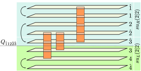
Figure 3: One can quantize the classical curve by choosing different orders of the sheets. Once an order (called path) is fixed the ${\mathsf{Q}}$ functions will correspond to the cuts crossing the line between two neighbor sheets. A ${\mathsf{Q}}$ function is not affected by the permutations of sheets above and below the line. Thus the ${\mathsf{Q}}$ function is uniquely determined by the subset of the sheets above the line and we denote it as $Q_{{\hat{1}}{{1}}{{2}}{\hat{2}}{\hat{3}}}$. For more formal definitions see section 4.3.

We will see that it is useful not to restrict ourselves to a single possible discretization (related to the quasi-classical quantization) of the curve but rather to consider all possible permutations of the sheets. These permutations can be denoted by sequences of indices labeling the sheets. In these notations, we denote the chosen ordering (grading) of sheets as ${\hat{1}}{{1}}{{2}}{\hat{2}}{\hat{3}}{{3}}{{4}}{\hat{4}}$.

The grading ${\hat{1}}{{1}}{{2}}{\hat{2}}{\hat{3}}{{3}}{{4}}{\hat{4}}$ has some obvious advantages in the ABA limit and we will use it as a canonical one.

The main motivation of this paper is the generalization of this solution to the full quantum case of the AdS${}_{5}/$CFT₄ Y-system valid for any operator and any $\lambda$. In the next section we show that at least the first part of this program – the general solution of the T-system (3) in the $\mathbb{T}$-hook, in terms of a finite number of functions of $u$ – the Baxter’s ${\mathsf{Q}}$-functions – can be fulfilled in a rather explicit form. The next step – finding the general analyticity properties of these functions and constructing the corresponding FiNLIE, will be the subject of a future work.

4 Solution of the full Hirota equation in $\mathbb{T}$-hook

Our goal here will be the construction of a general solution of Hirota equation (3) for the $(2|4|2)$ $\mathbb{T}$-hook, first in terms of the generating functional (GF) and then in explicit and finite form, in terms of the Wronskians – the finite determinants of ${\mathsf{Q}}$-functions.

4.1 Generating functional for the $\mathbb{T}$-hook

For given $T_{1,s}(u),\quad-\infty<s<\infty$, the general solution of (3) is given by the Bazhanov-Reshetikhin (BR) type formula

$$T_{a,s}=\det_{1\leqslant j,k\leqslant a}T_{1,s+j-k}^{[-a+k+j-1]}\;.$$ (34)

As was shown in [28, 29, 33], to solve Hirota equation in a $(M|N)$ fat hook the “symmetric” T-functions $T_{1,s}(u)$ should be generated by a special generating functional. In particular, for the $(2|2)$ fat hook, in the grading $(1|2|1)$ corresponding to the Kac-Dynkin diagram $\otimes\!\!-\!\!\odot\!\!-\!\!\otimes$, or to the $\{y_{{\hat{1}}}|x_{1},x_{2}|y_{{\hat{2}}}\}$ ordering of the eigenvalues of a twist parameter $g\in GL(2|2)$, we have the following generating functional

$$W={U}_{,{\hat{1}}}\,{U}_{{\hat{1}},{{1}}}^{-1}\,{U}_{{\hat{1}}{{1}},{{2}}}^{-1}\,{U}_{{\hat{1}}{{1}}{{2}},{\hat{2}}}=\sum_{s=-\infty}^{\infty}D^{s}T_{1,s}D^{s}$$ (35)

where

$${U}_{A}=(1-D\chi_{A}D),\qquad\qquad(D=e^{-\frac{i}{2}\partial_{u}})$$ (36)

with $A\subset I_{0}=\{{\hat{1}}|{{1}},{{2}}|{\hat{2}}\}$ being an arbitrary subset of the full set $I_{0}$, while
$\{\chi_{,{\hat{1}}}(u)|\chi_{{\hat{1}},{{1}}}(u),\chi_{{\hat{1}}{{1}},{{2}}}(u)|\chi_{{\hat{1}}{{1}}{{2}},{\hat{2}}}(u)\}$ are arbitrary functions of the spectral parameter $u$, replacing the group element eigenvalues $\{y_{{\hat{1}}}|x_{{{1}}},x_{{{2}}}|y_{{\hat{2}}}\}$ of the character generating function (15), whereas the generating parameter $t$ is replaced by the shift operator $D=e^{-\frac{i}{2}\partial_{u}}$. As was proposed in [32] in the case of a more general superalgebra $gl(M|N)$ (and demonstrated on the Fig.3), the labeling here follows the pattern of the Dynkin diagram in the grading $\otimes\!\!-\!\!\odot\!\!-\!\!\otimes$: we start from the l.h.s. of this diagram with $A=(,{\hat{1}})$ for the first factor in the l.h.s. of (35); then for the label $A$ of the second factor, one moves the comma one step to the right and adds new index after the comma, making $A=({\hat{1}},i)$. The choice of the index is related to the grading: when moving to the right of the Dynkin diagram we cross the fermionic node which means that we chose to add an entry from $I$ with a different grading than the previous $i$, say ${{1}}$, which gives for the second factor $A=({\hat{1}},{{1}}$); then we cross the bosonic node, which means that we should add an entree with the same grading as the last one, i.e. ${{2}}$, which gives for the label of the third factor $A=({\hat{1}}{{1}},{{2}})$, and finally, crossing the last fermionic node we get for the label of the last factor $A=({\hat{1}}{{1}}{{2}},{\hat{2}})$. This means that the subset $A$ represents a “path” by which it was reached starting from the l.h.s. of the Dynkin diagram. This will be the general rule of for more complicated algebras, and in particular $u(2,2|4)$.

To calculate $T_{a,s}(u)$ in terms of these functions we formally expand the l.h.s. in powers of the shift operator $D=e^{-\frac{i}{2}\partial_{u}}$ and compare the coefficients with the r.h.s. The formal proof can be found in [28, 29, 33], but it is easy to convince oneself on Mathematica that the $T$-functions generated from $T_{1,s}$ by (34) are zero outside of the $(2|2)$ fat hook.

What is the solution for the $\mathbb{T}$-hook of $u(2,2|4)$? We can read it off from the generating function for the characters of $u(2,2|4)$ given by eqs.(15)-(16). Note that the integration contour prescription in (16) means that we can generate the $u(2,2|4)$ characters by expanding the first factor in the r.h.s. of (15) in powers of $t$, and the second factor – in powers of $\frac{1}{t}$, and then extract from the product $T_{1,s}$ as a coefficient in front of the power $t^{s}$. The result is given in terms of infinite sums, and not polynomials in the eigenvalues, signalling that we deal with infinite-dimensional irreps of $u(2,2|4)$ [44, 34, 45].

Similarly to the case $gl(2|2)$ described above, we can try as a quantum generalization of equation (3) for the $(2|4|2)$ $\mathbb{T}$-hook, for the particular grading of the eigenvalues $\{y_{\hat{1}}|x_{{1}},x_{{2}}|y_{\hat{2}},y_{\hat{3}}|x_{{3}},x_{{4}}|y_{\hat{4}}\}$ corresponding to the Kac-Dynkin diagram $\otimes\!\!-\!\!\odot\!\!-\!\!\otimes\!\!-\!\!\odot\!\!-\!\!\otimes\!\!-\!\!\odot\!\!-\!\!\otimes$, the following generating functional [34]

$$W = \left[V_{\hat{1}}\,V_{{{1}}}^{-1}\,V_{{{2}}}^{-1}\,V_{{\hat{2}}}\right]_{+}\times\left[V_{{\hat{3}}}\,V_{{{3}}}^{-1}\,V_{{{4}}}^{-1}\,V_{{\hat{4}}}\right]_{-}\!\!=\!\!\sum_{s=-\infty}^{\infty}D^{s}T_{1,s}D^{s}$$ (37)

where we introduced, to make the formula less bulky, the notations $V_{j}=1-D\xi_{j}D$ with

$$\xi_{{\hat{1}}} = \chi_{\hat{1}}\,\qquad\quad\,\,\,\xi_{{{1}}}=\chi_{{\hat{1}},{{1}}}\,\qquad\quad\xi_{{2}}=\chi_{{\hat{1}}{{1}},{{2}}}\,\qquad\xi_{\hat{2}}=\chi_{{\hat{1}}{{1}}{{2}},{\hat{2}}}\,$$

$$\xi_{{\hat{3}}} = \chi_{{\hat{1}}{{1}}{{2}}{\hat{2}},{\hat{3}}}\,\qquad\xi_{{3}}=\chi_{{\hat{1}}{{1}}{{2}}{\hat{2}}{\hat{3}},{{3}}}\,\quad\xi_{{{4}}}=\chi_{{\hat{1}}{{1}}{{2}}{\hat{2}}{\hat{3}}{{3}},{{4}}}\,\quad\xi_{\hat{4}}=\chi_{{\hat{1}}{{1}}{{2}}{\hat{2}}{\hat{3}}{{3}}{{4}},{\hat{4}}}\;.$$ (38)

We label the functions $\xi_{j}$ only by the last index in the subset $A$ of $\chi_{A}$ having in mind the particular grading, or nesting path. By definition, we expand inside $\left[\dots\right]_{+}$ and $\left[\dots\right]_{-}$ w.r.t. the positive and negative powers of $D$ respectively and then calculate the functions $T_{1,s},\,\,-\infty<s<\infty$, comparing the powers of $D$ on both sides of the eq.(37). To restore the rest of $T_{a,s}$ we can use again (34).

The formal proof of the fact that (34),(37) represents the complete solution of Hirota equation within the $\mathbb{T}$-hook will be published elsewhere, but, again, it is easy to convince oneself in the correctness of this formula on Mathematica.

The representation (37) is already a considerable advance w.r.t. the original Y-system (1) since its solution is now parameterized in terms of a finite number of functions $\xi_{j}$. A solution of Hirota equation is now parameterized by $8$ arbitrary independent functions $\xi_{j}$ entering the generating functional (37). Moreover in this form the passage to the general strong coupling solution found in [13] is straightforward – in the strong coupling limit the shift operator $D$ can be replaced by a formal scalar expansion parameter $t$ whereas $\xi_{j}$ should become the eigenvalues of the classical monodromy matrix. This solution is quite useful for various applications. Note however that as the result we get infinite series, signaling that we deal with infinite dimensional representations of $U(2,2|4)$. In the next section, we will show that these infinite series can be “miraculously” converted to the explicit finite dimensional Wronskian determinants.

4.2 QQ-relations

To find the Wronskian solution we have to choose a good parameterization for all these 8 functions (4.1). The formalism of [28, 29, 34, 33, 32] aimed at the derivation of Bethe equations as a condition of analyticity, i.e. polynomiality, of the T-functions, as well as the form of the classical finite gap solution (33) suggests that the best parameterization would be in terms of the ${\mathsf{Q}}$-functions (a-la Baxter). As it was explained in sections 3.2 and 4.1 and on the Fig.3, all the $2^{8}$ ${\mathsf{Q}}$-functions can be labeled by all possible subsets from the full set $I_{0}=\{{{1}},{{2}},{{3}},{{4}}|{\hat{1}},{\hat{2}},{\hat{3}},{\hat{4}}\}$.

The monomials of the generating functional can be conveniently parameterized in terms of 8 Baxter’s ${\mathsf{Q}}$-functions as follows:

$$\begin{array}[]{llllll}\xi_{{\hat{1}}}=\frac{{\mathsf{Q}}_{\emptyset}^{++}{\mathsf{Q}}_{{\hat{1}}}^{-}}{{\mathsf{Q}}_{\emptyset}{\mathsf{Q}}_{{\hat{1}}}^{+}}\;,&\xi_{{{1}}}=\frac{{\mathsf{Q}}_{{\hat{1}}}^{-}{\mathsf{Q}}_{{\hat{1}}{{1}}}^{++}}{{\mathsf{Q}}_{{\hat{1}}}^{+}{\mathsf{Q}}_{{\hat{1}}{{1}}}}\;,&\xi_{{{2}}}=\frac{{\mathsf{Q}}_{{\hat{1}}{{1}}}^{--}{\mathsf{Q}}_{{\hat{1}}{{1}}{{2}}}^{+}}{{\mathsf{Q}}_{{\hat{1}}{{1}}}{\mathsf{Q}}_{{\hat{1}}{{1}}{{2}}}^{-}}\;,&\xi_{{\hat{2}}}=\frac{{\mathsf{Q}}_{{\hat{1}}{{1}}{{2}}}^{+}{\mathsf{Q}}_{{\hat{1}}{{1}}{{2}}{\hat{2}}}^{--}}{{\mathsf{Q}}_{{\hat{1}}{{1}}{{2}}}^{-}{\mathsf{Q}}_{{\hat{1}}{{1}}{{2}}{\hat{2}}}}\;,\\ {\xi}_{{\hat{4}}}=\frac{{\mathsf{Q}}_{{\hat{1}}{{1}}{{2}}{\hat{2}}{\hat{3}}{{3}}{{4}}{\hat{4}}}^{--}{\mathsf{Q}}_{{\hat{1}}{{1}}{{2}}{\hat{2}}{\hat{3}}{{3}}{{4}}}^{+}}{{\mathsf{Q}}_{{\hat{1}}{{1}}{{2}}{\hat{2}}{\hat{3}}{{3}}{{4}}{\hat{4}}}{\mathsf{Q}}_{{\hat{1}}{{1}}{{2}}{\hat{2}}{\hat{3}}{{3}}{{4}}}^{-}}\;,&{\xi}_{{{4}}}=\frac{{\mathsf{Q}}_{{\hat{1}}{{1}}{{2}}{\hat{2}}{\hat{3}}{{3}}{{4}}}^{+}{\mathsf{Q}}_{{\hat{1}}{{1}}{{2}}{\hat{2}}{\hat{3}}{{3}}}^{--}}{{\mathsf{Q}}_{{\hat{1}}{{1}}{{2}}{\hat{2}}{\hat{3}}{{3}}{{4}}}^{-}{\mathsf{Q}}_{{\hat{1}}{{1}}{{2}}{\hat{2}}{\hat{3}}{{3}}}}\;,&{\xi}_{{{3}}}=\frac{{\mathsf{Q}}_{{\hat{1}}{{1}}{{2}}{\hat{2}}{\hat{3}}{{3}}}^{++}{\mathsf{Q}}_{{\hat{1}}{{1}}{{2}}{\hat{2}}{\hat{3}}}^{-}}{{\mathsf{Q}}_{{\hat{1}}{{1}}{{2}}{\hat{2}}{\hat{3}}{{3}}}{\mathsf{Q}}_{{\hat{1}}{{1}}{{2}}{\hat{2}}{\hat{3}}}^{+}}\;,&{\xi}_{{\hat{3}}}=\frac{{\mathsf{Q}}_{{\hat{1}}{{1}}{{2}}{\hat{2}}{\hat{3}}}^{-}{\mathsf{Q}}_{{\hat{1}}{{1}}{{2}}{\hat{2}}}^{++}}{{\mathsf{Q}}_{{\hat{1}}{{1}}{{2}}{\hat{2}}{\hat{3}}}^{+}{\mathsf{Q}}_{{\hat{1}}{{1}}{{2}}{\hat{2}}}}\;.\end{array}$$ (39)

The way we perform this parameterization for the functions $\chi_{A}$ (see the definition (4.1)) in terms of the ${\mathsf{Q}}$-functions is completely defined by the chosen nesting (grading) path and is simply given by $\chi_{I,j}=\frac{{\mathsf{Q}}_{I}^{[k+2\sigma]}}{{\mathsf{Q}}_{I}^{[k]}}\frac{{\mathsf{Q}}_{I,j}^{[k-\sigma]}}{{\mathsf{Q}}_{I,j}^{[k+\sigma]}}$ where ${\mathsf{Q}}_{I}^{[k]}$ in the denominator is the same as the last ${\mathsf{Q}}$ in the denominator of $\chi_{I}$, $\sigma=\pm 1$ is chosen so that the first ratio in $\chi_{I,j}$ is the same as the last ratio in $\chi_{I}$ when we change the grading passing from $(I,i)$ to $(Ii,j)$, and $\sigma$ is opposite otherwise. All such nesting paths for the case of $su(2|2)$ are shown on the Hasse diagram in Fig.4.

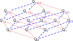
Figure 4: Hasse diagram for $gl(2|2)$ (cf. [32]): To construct the generating functional (35) we move along any path starting at the node $\emptyset$ and ending at the node ${{1}}{{2}}{\hat{1}}{\hat{2}}$. Each line corresponds to adding the next $U$-factor (or $V$-factor in (37) for the $(2,2|4)$ case) with one extra index. The dashed blue (resp. dotted red) lines stand for adding a “bosonic” (resp. fermionic) index, and each local change of the nesting path at some rectangular facet of the diagram gives rise to the $QQ$-relations (40), (41). The equation (41) (resp. (40)) corresponds to the facets having $2$ “bosonic” lines and $2$ “fermionic” lines (resp to the facets having all $4$ “bosonic” or all $4$ “fermionic” lines).

All that means that the labeling of ${\mathsf{Q}}$-functions follows the nesting path. However, it is clear from the Fig.3 and the explanations in sec.3.2 that these $Q$-functions do not depend on the order of indices in the path up to a sign: a permutation of indices multiplies the ${\mathsf{Q}}$-function by the signature of the permutation.

Moreover, all these $2^{8}=256$ ${\mathsf{Q}}$-functions are not independent and can be expressed through a chosen basis of 8 ${\mathsf{Q}}$-functions. The rest of them are related to those 8 by the so called QQ-relations [35, 33, 59, 57, 30, 55, 31]:

$${\mathsf{Q}}_{I}{\mathsf{Q}}_{I,ij}={\mathsf{Q}}_{I,i}^{[{\mathsf{p}}_{i}]}{\mathsf{Q}}_{I,j}^{[-{\mathsf{p}}_{i}]}-{\mathsf{Q}}_{I,i}^{[-{\mathsf{p}}_{i}]}{\mathsf{Q}}_{I,j}^{[{\mathsf{p}}_{i}]}\qquad\text{for}\qquad{\mathsf{p}}_{i}={\mathsf{p}}_{j},\\$$ (40)

$${\mathsf{Q}}_{I,i}{\mathsf{Q}}_{I,j}={\mathsf{Q}}_{I}^{[-{\mathsf{p}}_{i}]}{\mathsf{Q}}_{I,ij}^{[{\mathsf{p}}_{i}]}-{\mathsf{Q}}_{I}^{[{\mathsf{p}}_{i}]}{\mathsf{Q}}_{I,ij}^{[-{\mathsf{p}}_{i}]}\qquad\text{for}\qquad{\mathsf{p}}_{i}=-{\mathsf{p}}_{j}.$$ (41)

$$\textrm{where}\qquad{\mathsf{p}}_{i}=+1,\qquad i\in\{{{1}},{{2}},{{3}},{{4}}\}\qquad\textrm{and}\qquad{\mathsf{p}}_{{\hat{\imath}}}=-1,\qquad{\hat{\imath}}\in\{{\hat{1}},{\hat{2}},{\hat{3}},{\hat{4}}\}$$ (42)

These QQ-relations can be obtained from the fact that the relabeling of $\chi$-functions and ${\mathsf{Q}}$-functions in (37) by changing the nesting path does not change the generating functional. This change occurs from the commutation of two consecutive $U$-factors in the generating functional. Following the nesting path $(I,i)\to(I,i,j)$ should give the same generating functional in 37 as the path $(I,j)\to(I,j,i)$:

$$V_{I,i}^{-{\mathsf{p}}_{i}}V_{I,ij}^{-{\mathsf{p}}_{j}}=V_{I,j}^{-{\mathsf{p}}_{j}}V_{I,ji}^{-{\mathsf{p}}_{i}}$$ (43)

which gives both “bosonic” and “fermionic” QQ-relations (40) and (41).

Let us note that the dependence on the general ($u$-independent) twist matrix
$g={\rm diag}\{z_{\hat{1}}|z_{{1}},z_{{2}}|z_{\hat{2}},z_{\hat{3}}|z_{{3}},z_{{4}}|z_{\hat{4}}\}\in GL(4|4)$, useful for some applications, such as the $\beta$-deformed version of the AdS₅/CFT₄ duality, can be easily introduced into the $\mathbb{T}$-hook solution (37) by a certain simple rescaling of all ${\mathsf{Q}}$-functions.

4.3 Explicit Wronskian formulae for $\mathbb{T}$-hook

Now we can formulate the central result of this paper – the determinant formulae for the complete solution of the Hirota equation ($T$-system) (3) within the $(2,2|4)$ $\mathbb{T}$-hook. They are written in a gauge where ${\mathsf{Q}}_{\emptyset}=1$, and the whole set of non-zero T-functions is given by the following three formulas

$${\mathsf{T}}_{1,s} =+{\mathsf{Q}}_{{{1}}}^{[s]}{\mathsf{Q}}_{\overline{{{1}}}}^{[-s]}-{\mathsf{Q}}_{{{2}}}^{[s]}{\mathsf{Q}}_{\overline{{{2}}}}^{[-s]}\;\;,\;\;s\geqslant+1$$

$${\mathsf{T}}_{2,s} =+{\mathsf{Q}}_{{{1}}{{2}}}^{[s]}{\mathsf{Q}}_{\overline{{{1}}{{2}}}}^{[-s]}\;\;,\;\;s\geqslant+2$$ (44)

$${\mathsf{T}}_{a,+2} =+{\mathsf{Q}}_{{{1}}{{2}}}^{[a]}{\mathsf{Q}}_{\overline{{{1}}{{2}}}}^{[-a]}\;\;,\;\;a\geqslant 2$$

$${\mathsf{T}}_{a,+1} =(-1)^{a+1}\left({\mathsf{Q}}_{{{1}}{{2}}{\hat{1}}}^{[a]}{\mathsf{Q}}_{\overline{{{1}}{{2}}{\hat{1}}}}^{[-a]}-{\mathsf{Q}}_{{{1}}{{2}}{\hat{2}}}^{[a]}{\mathsf{Q}}_{\overline{{{1}}{{2}}{\hat{2}}}}^{[-a]}+{\mathsf{Q}}_{{{1}}{{2}}{\hat{3}}}^{[a]}{\mathsf{Q}}_{\overline{{{1}}{{2}}{\hat{3}}}}^{[-a]}-{\mathsf{Q}}_{{{1}}{{2}}{\hat{4}}}^{[a]}{\mathsf{Q}}_{\overline{{{1}}{{2}}{\hat{4}}}}^{[-a]}\right)\;\;,\;\;a\geqslant 1$$

$${\mathsf{T}}_{a,0} =+{\mathsf{Q}}_{{{1}}{{2}}{\hat{1}}{\hat{2}}}^{[a]}{\mathsf{Q}}_{{{4}}{{3}}{\hat{4}}{\hat{3}}}^{[-a]}-{\mathsf{Q}}_{{{1}}{{2}}{\hat{1}}{\hat{3}}}^{[a]}{\mathsf{Q}}_{{{4}}{{3}}{\hat{4}}{\hat{2}}}^{[-a]}+{\mathsf{Q}}_{{{1}}{{2}}{\hat{1}}{\hat{4}}}^{[a]}{\mathsf{Q}}_{{{4}}{{3}}{\hat{3}}{\hat{2}}}^{[-a]}+{\mathsf{Q}}_{{{1}}{{2}}{\hat{2}}{\hat{3}}}^{[a]}{\mathsf{Q}}_{{{4}}{{3}}{\hat{4}}{\hat{1}}}^{[-a]}-{\mathsf{Q}}_{{{1}}{{2}}{\hat{2}}{\hat{4}}}^{[a]}{\mathsf{Q}}_{{{4}}{{3}}{\hat{3}}{\hat{1}}}^{[-a]}+{\mathsf{Q}}_{{{1}}{{2}}{\hat{3}}{\hat{4}}}^{[a]}{\mathsf{Q}}_{{{4}}{{3}}{\hat{2}}{\hat{1}}}^{[-a]}$$

$${\mathsf{T}}_{a,-1}{} =(-1)^{a+1}\left({\mathsf{Q}}_{\overline{{{4}}{{3}}{\hat{4}}}}^{[a]}{\mathsf{Q}}_{{{4}}{{3}}{\hat{4}}}^{[-a]}-{\mathsf{Q}}_{\overline{{{4}}{{3}}{\hat{3}}}}^{[a]}{\mathsf{Q}}_{{{4}}{{3}}{\hat{3}}}^{[-a]}+{\mathsf{Q}}_{\overline{{{4}}{{3}}{\hat{2}}}}^{[a]}{\mathsf{Q}}_{{{4}}{{3}}{\hat{2}}}^{[-a]}-{\mathsf{Q}}_{\overline{{{4}}{{3}}{\hat{1}}}}^{[a]}{\mathsf{Q}}_{{{4}}{{3}}{\hat{1}}}^{[-a]}\right)\;\;,\;\;a\geqslant 1$$

$${\mathsf{T}}_{a,-2} ={\mathsf{Q}}_{\overline{{{4}}{{3}}}}^{[a]}{\mathsf{Q}}_{{{4}}{{3}}}^{[-a]}\;\;,\;\;a\geqslant 2$$

$${\mathsf{T}}_{2,s} =+{\mathsf{Q}}_{\overline{{{4}}{{3}}}}^{[-s]}{\mathsf{Q}}_{{{4}}{{3}}}^{[s]}\;\;,\;\;s\leqslant-2$$

$${\mathsf{T}}_{1,s} =+{\mathsf{Q}}_{\overline{{{4}}}}^{[-s]}{\mathsf{Q}}_{{{4}}}^{[s]}-{\mathsf{Q}}_{\overline{{{3}}}}^{[-s]}{\mathsf{Q}}_{{{3}}}^{[s]}\;\;,\;\;s\leqslant-1$$

$${\mathsf{T}}_{0,s} =+{\mathsf{Q}}_{\overline{\emptyset}}^{[-s]}\;$$

where the bar over the indices denotes the complementary set, for instance ${\mathsf{Q}}_{\overline{{{1}}{{2}}}}={\mathsf{Q}}_{{{3}}{{4}}{\hat{1}}{\hat{2}}{\hat{3}}{\hat{4}}}$. Note that this solution obeys the following properties:

$$(\partial_{u}-2i\partial_{s}){\mathsf{T}}_{0,s}(u)=0,\qquad{\mathsf{T}}_{k,2}={\mathsf{T}}_{2,k},\qquad{\mathsf{T}}_{k,-2}={\mathsf{T}}_{2,-k},\qquad k\geqslant 2.$$ (45)

That means that we have imposed three out of four possible gauge constraints (5).

Using the determinant formulas (69) and (70) solving the QQ-relations and the Laplace expansion formula for the determinants it is also possible to rewrite T-functions in various determinant forms. For example, we have the following $4\times 4$ and $2\times 2$ determinant expressions reminding the character formula (20): For the upper strip $a\geqslant|s|$ of the $\mathbb{T}$-hook we can represent $T_{a,s}$ as a $4\times 4$ determinant

$${\mathsf{T}}_{a,s} =\frac{(-1)^{sa}}{{\cal(F}_{1-s}\circ{\mathsf{Q}}_{{{1}}{{2}}}^{[a]}{\cal)(F}_{1+s}\circ{\mathsf{Q}}_{{{3}}{{4}}}^{[-a]})}\begin{vmatrix}({\mathsf{Q}}_{{{1}}{{2}},j}^{[a-s-2i+3]})_{1\leqslant i\leqslant 2-s,{\hat{1}}\leqslant j\leqslant{\hat{4}}}\\ ({\mathsf{Q}}_{{{3}}{{4}},j}^{[-a+s+3-2i]})_{1\leqslant i\leqslant 2+s,{\hat{1}}\leqslant j\leqslant{\hat{4}}}\\ \end{vmatrix}.$$ (46)

and for the right strip ($s\geqslant a\geqslant 0$)

$${\mathsf{T}}_{a,s} =\frac{-1}{{\cal F}_{1-a}\circ{\mathsf{Q}}_{{{3}}{{4}}{\hat{1}}{\hat{2}}{\hat{3}}{\hat{4}}}^{[-s]}}\begin{vmatrix}\left({\mathsf{Q}}_{j,{{3}}{{4}}{\hat{1}}{\hat{2}}{\hat{3}}{\hat{4}}}^{[-s+a-3+2k]}\right)_{\begin{subarray}{c}{{1}}\leqslant j\leqslant 2\\ 1\leqslant k\leqslant 2-a\end{subarray}}&\left({\mathsf{Q}}_{j}^{[s-a+2k-1]}\right)_{\begin{subarray}{c}{{1}}\leqslant j\leqslant 2\\ 1\leqslant k\leqslant a\end{subarray}}\\ \end{vmatrix}$$ (47)

and the left strip ($-s\geqslant a\geqslant 0$):

$${\mathsf{T}}_{a,s} =\frac{-1}{{\cal F}_{1-a}\circ{\mathsf{Q}}_{{{1}}{{2}}{\hat{1}}{\hat{2}}{\hat{3}}{\hat{4}}}^{[-s]}}\begin{vmatrix}\left({\mathsf{Q}}_{j}^{[s-a+2k-1]}\right)_{\begin{subarray}{c}{{3}}\leqslant j\leqslant{{4}}\\ 1\leqslant k\leqslant a\end{subarray}}&\left({\mathsf{Q}}_{{{1}}{{2}},j,{\hat{1}}{\hat{2}}{\hat{3}}{\hat{4}}}^{[-s+a-3+2k]}\right)_{\begin{subarray}{c}{{3}}\leqslant j\leqslant{{4}}\\ 1\leqslant k\leqslant 2-a\end{subarray}}\\ \end{vmatrix}$$ (48)

as $2\times 2$ determinants.

Note that the above $T$-functions are taken in a different gauge than the $T$-functions of the generating functional. They are related as ${\mathsf{T}}^{[0]}_{a,s}={\mathsf{Q}}_{\emptyset}^{[s-a]}{\mathsf{Q}}_{{{1}}{{2}}{{3}}{{4}}{\hat{1}}{\hat{2}}{\hat{3}}{\hat{4}}}^{[-s+a]}T^{[0]}_{a,s}$, where ${\mathsf{Q}}_{\emptyset}=1$ in our normalization. It is not difficult to see that these formulas solve indeed the Hirota equation in $\mathbb{T}$-hook. Indeed, the Wronskian determinants (46), (47) and (48) have similar structures as the ones solving the Hirota equations in the infinite strips of a sizes $N=4,2,2$, respectively (see [27], and its applications [20]).

It is easy to see that to saw the three semi-infinite strips together into the full $\mathbb{T}$-hook it is enough to prove that the Wronskian solution satisfies four Hirota equations corresponding to the nodes $(a,s)=(\pm 1,\pm 2)$. This can be done straightforwardly.

There exist many possible determinant representations for the solution. In the next subsection we will show, as an example, how to write every ${\mathsf{Q}}$-function explicitly in terms of a basis of 8 ${\mathsf{Q}}$ functions.

4.4 A basis for ${\mathsf{Q}}$ functions

The aim of this subsection is to show that it is possible to express explicitly and in a finite form all the T-functions of the $\mathbb{T}$-hook in terms of a basis of 8 Q-functions, at least for a particular choice of this basis.

As we already mentioned, all the T-functions can be expressed, as the general solution of Hirota bilinear difference equation, through 8 independent functions. Already the generating functional (37) performs this task but, unfortunately, every T-function is expressed only by an infinite series in terms of 8 $\xi$-functions (4.1), organized in powers of wrapping. Another solution involving infinite series was recently proposed in [37] which is closely related to the generating functional (37) presented several years ago [34] in a different context. Their parameterization (39) in terms of 8 particular Q-functions does not immediately lead to finite expressions for the T-functions since to express the Q-functions of (44) in terms of these 8 Q-functions we need to solve the appropriate QQ-relations which, a priori, will lead again to the inversion of some finite difference operators, and hence to some infinite products.

Nevertheless, we will show here that all the ${\mathsf{Q}}$ functions can be explicitly expressed in a finite form as Wronskian determinants in terms of a particular basis $\mathcal{B}_{1}=\{{\mathsf{Q}}_{{{1}}},\linebreak[1]{\mathsf{Q}}_{{{2}}},\linebreak[1]{\mathsf{Q}}_{{{3}}},\linebreak[1]{\mathsf{Q}}_{{{4}}},\linebreak[1]q_{{\hat{1}}},\linebreak[1]q_{{\hat{2}}},\linebreak[1]q_{{\hat{3}}},q_{\hat{4}}\}$ where $q_{\hat{f}}={\mathsf{Q}}_{\overline{{\hat{f}}}}/{{\mathsf{Q}}_{\overline{\emptyset}}^{+}}$. First, the bosonization trick (see Appendix A) says that by relabelling all the ${\mathsf{Q}}$-functions as ${\mathsf{Q}}_{I}=\tilde{{\mathsf{Q}}}_{I\triangle B}$, defined by (72), one gets $\tilde{\mathsf{Q}}$-functions which obey for any indices (for the gradings with or without hats) only the “bosonic” QQ-relation (40) with ${\mathsf{p}}_{i}={\mathsf{p}}_{j}=-1,\forall i,j$. In other words, the functions $\tilde{\mathsf{Q}}$ don’t distinguish bosonic and fermionic indices, and all the $\tilde{\mathsf{Q}}$-functions with more than one index can be expressed through one-index $\tilde{\mathsf{Q}}$-functions by standard bosonic determinants, namely

$${\tilde{\mathsf{Q}}}_{{i_{1},i_{2},\cdots i_{N}}}=\frac{\left|\left(\tilde{\mathsf{Q}}_{{i_{k}}}^{[-N-1+2l]}\right)_{1\leqslant k,l\leqslant N}\right|}{{\cal F}_{N-1}\circ\tilde{\mathsf{Q}}_{\emptyset}}$$ (49)

In this manner, every ${\mathsf{Q}}$-function can be represented as a determinant of the Q-functions of the set $\mathcal{B}_{2}=\{{\tilde{\mathsf{Q}}}_{\emptyset},{\tilde{\mathsf{Q}}}_{{{1}}},{\tilde{\mathsf{Q}}}_{{{2}}},{\tilde{\mathsf{Q}}}_{{{3}}},{\tilde{\mathsf{Q}}}_{{{4}}},{\tilde{\mathsf{Q}}}_{{\hat{1}}},{\tilde{\mathsf{Q}}}_{{\hat{2}}},{\tilde{\mathsf{Q}}}_{{\hat{3}}},{\tilde{\mathsf{Q}}}_{{\hat{4}}}\}$.

We will show now that we can express  all ${\mathsf{Q}}$-functions through 8 functions of the set $\mathcal{B}_{1}$ in an  explicit and  finite form. On the other hand, $\mathcal{B}_{2}$ contains $9$ ${\mathsf{Q}}$-functions, which are not all independent. Due to the Plücker relations among various ${\mathsf{Q}}$-functions given in the Appendix A, these $9$ functions can be expressed as determinants of $8$ independent functions of the basis $\mathcal{B}_{1}$ as follows:

$${\tilde{\mathsf{Q}}}_{\emptyset} =\left|{\left({\mathsf{Q}}_{i}^{[j]}\right)}_{\begin{subarray}{c}{{1}}\leqslant i\leqslant{{4}}\\ j=3,1,-1,-3\end{subarray}}\right|$$ (50)

$$\tilde{{\mathsf{Q}}}_{b} =\left|\left({{\mathsf{Q}}_{i}^{[j]}}\right)_{\begin{subarray}{c}{{1}}\leqslant i\leqslant{{4}};~{}i\neq b\\ j=2,0,-2\end{subarray}}\right|\, {{1}}\leqslant b\leqslant{{4}}$$ (51)

$${\tilde{\mathsf{Q}}}_{{\hat{f}}} ={\mathsf{Q}}_{\overline{\emptyset}}^{[3]}\left|\left(q_{\hat{\imath}}^{[j]}\right)_{\begin{subarray}{c}{\hat{1}}\leqslant{\hat{\imath}}\leqslant{\hat{4}};~{}{\hat{\imath}}\neq{\hat{f}}\\ j=2,0,-2\end{subarray}}\right| {\hat{1}}\leqslant{\hat{f}}\leqslant{\hat{4}}$$ (52)

$$\mathrm{where}\qquad{\mathsf{Q}}_{\overline{\emptyset}} ={\tilde{\mathsf{Q}}}_{\emptyset}^{[-4]}\Big{/}\left|\left(q_{\hat{\imath}}^{[j]}\right)_{\begin{subarray}{c}{\hat{1}}\leqslant{\hat{\imath}}\leqslant{\hat{4}}\\ j=-1,-3,-5,-7\end{subarray}}\right| q_{\hat{f}}={\mathsf{Q}}_{\overline{{\hat{f}}}}/{{\mathsf{Q}}_{\overline{\emptyset}}^{+}}$$ (53)

The relations (50) and (51), for $\tilde{\mathsf{Q}}_{\emptyset}\equiv{\mathsf{Q}}_{{{1}}{{2}}{{3}}{{4}}}$ and $(\tilde{\mathsf{Q}}_{{{1}}},\tilde{\mathsf{Q}}_{{{2}}},\tilde{\mathsf{Q}}_{{{3}}},\tilde{\mathsf{Q}}_{{{4}}})\equiv({\mathsf{Q}}_{{{2}}{{3}}{{4}}},\linebreak[1]{\mathsf{Q}}_{{{1}}{{3}}{{4}}},\linebreak[1]{\mathsf{Q}}_{{{1}}{{2}}{{4}}},\linebreak[1]{\mathsf{Q}}_{{{1}}{{2}}{{3}}})$ are simply the determinant solution of bosonic Plücker QQ-relations (69) (in the gauge ${\mathsf{Q}}_{\emptyset}=1$). In the same manner as the bosonization trick, the transformation $I\mapsto\bar{I}$ simply exchanges the gradings of all indices: so that the same bosonic determinant gives for instance

$${\mathsf{Q}}_{\overline{{\hat{1}}{\hat{2}}{\hat{3}}}}=\frac{\det_{\begin{subarray}{c}{\hat{1}}\leqslant{\hat{\imath}}\leqslant{\hat{3}}\\ j=2,0,-2\end{subarray}}\left({{\mathsf{Q}}_{\overline{{\hat{\imath}}}}^{[j]}}\right)}{{\mathsf{Q}}^{+}_{\overline{\emptyset}}{\mathsf{Q}}^{-}_{\overline{\emptyset}}}\;\;,\;\;\text{and}\;\;{\mathsf{Q}}_{\overline{{\hat{1}}{\hat{2}}{\hat{3}}{\hat{4}}}}=\frac{\det_{\begin{subarray}{c}{\hat{1}}\leqslant{\hat{\imath}}\leqslant{\hat{4}}\\ j=3,1,-1,-3\end{subarray}}\left({{\mathsf{Q}}_{\overline{{\hat{\imath}}}}^{[j]}}\right)}{{\cal F}_{3}\circ{\mathsf{Q}}_{\overline{\emptyset}}}\;.$$ (54)

Due to the definitions $({\tilde{\mathsf{Q}}}_{{\hat{1}}},{\tilde{\mathsf{Q}}}_{{\hat{2}}},{\tilde{\mathsf{Q}}}_{{\hat{3}}},{\tilde{\mathsf{Q}}}_{{\hat{4}}},{\tilde{\mathsf{Q}}}_{\emptyset})=({\mathsf{Q}}_{\overline{{\hat{2}}{\hat{3}}{\hat{4}}}},{\mathsf{Q}}_{\overline{{\hat{1}}{\hat{3}}{\hat{4}}}},{\mathsf{Q}}_{\overline{{\hat{1}}{\hat{2}}{\hat{4}}}}{\mathsf{Q}}_{\overline{{\hat{1}}{\hat{2}}{\hat{3}}}},{\mathsf{Q}}_{\overline{{\hat{1}}{\hat{2}}{\hat{3}}{\hat{4}}}})$, these determinants are easily recast into the formulae (52) and (53).

In this way, we fulfilled the task of this subsection: all ${\mathsf{T}}$-functions inside the $\mathbb{T}$-hook can be expressed through 8 (ratios of) ${\mathsf{Q}}$-functions.

The whole procedure is illustrated in the attached Mathematica file, which for instance computes the expression of any ${\mathsf{Q}}$-function in terms of the basis $\mathcal{B}_{1}$.

5 Asymptotic expressions for the generating functional and ${\mathsf{Q}}$ functions

Now we will demonstrate our generating functional and Wronskian solutions of the AdS/CFT Y-system in the asymptotic, large size limit $L\to\infty$. We will present the asymptotic expressions of the relevant $\chi$- and ${\mathsf{Q}}$-functions. All other ${\mathsf{Q}}$-functions can be expressed through the basic ones through the Wronskian relations described above. Although it will be just a recasting of the ABA formulas of [62] we feel that this Wronskian formulation is a right step in the direction of the derivation of the finite $L$ system of FiNLIE’s for the planar AdS/CFT spectrum.

5.1 Asymptotic limit for the generating functional

In the asymptotic limit the expressions for $\xi$-functions entering the generating functional (36),(37) can be written explicitly in terms of the ABA Bethe roots. Namely, expliciting the ${\mathsf{Q}}$-functions in the general expressions (39) we write [13, 43] (see also [63])

$$\xi_{\hat{1}}\simeq H{\overline{F}}^{+}\frac{B_{3}^{-}R_{1}^{-}}{B_{3}^{+}R_{1}^{+}}\;,\;\xi_{1}\simeq H\frac{B_{3}^{-}R_{1}^{-}Q_{2}^{++}}{B_{3}^{+}R_{1}^{+}Q_{2}}\;\;,\;\;\xi_{2}\simeq H\frac{B_{1}^{+}R_{3}^{+}Q_{2}^{--}}{B_{1}^{-}R_{3}^{-}Q_{2}}\;\;,\;\;\xi_{\hat{2}}\simeq H\frac{B_{1}^{+}R_{3}^{+}}{B_{1}^{-}R_{3}^{-}}F^{-}$$

$$\xi_{\hat{4}}\simeq{\overset{\multimap}{H}}{}\frac{1}{{\overline{F}}^{-}}\frac{B_{5}^{+}R_{7}^{+}}{B_{5}^{-}R_{7}^{-}}\;\;,\;\;\xi_{4}\simeq{\overset{\multimap}{H}}{}\frac{B_{5}^{+}R_{7}^{+}Q_{6}^{--}}{B_{5}^{-}R_{7}^{-}Q_{6}}\;\;,\;\;\xi_{3}\simeq{\overset{\multimap}{H}}{}\frac{Q_{6}^{++}B_{7}^{-}R_{5}^{-}}{Q_{6}B_{7}^{+}R_{5}^{+}}\;\;,\;\;\xi_{\hat{3}}\simeq{\overset{\multimap}{H}}{}\frac{B_{7}^{-}R_{5}^{-}}{B_{7}^{+}R_{5}^{+}}\frac{1}{F^{+}}$$ (55)

where

$$F=\frac{R^{(-)}}{R^{(+)}}\;\;,\;\;{\overline{F}}=\frac{B^{(+)}}{B^{(-)}}$$ (56)

and

$$H=\left(\frac{x^{-}}{x^{+}}\right)^{\tfrac{L}{2}}\frac{B^{(+)+}}{B^{(+)-}}S(u)\;\;,\;\;{\overset{\multimap}{H}}{}=\left(\frac{x^{+}}{x^{-}}\right)^{\tfrac{L}{2}}\frac{B^{(-)-}}{B^{(-)+}}\frac{1}{S(u)}$$ (57)

By ${\overline{A}}$ and ${\overset{\multimap}{A}}{}$ we denote the complex conjugations of $A$ in the mirror and physical sheets, respectively (see the definition in [41, 2]).

Note that in the $L\to\infty$ limit the first $4$ $\xi$’s are suppressed in the mirror sheet whereas the last $4$ are exponentially large. The expansion of the generating series can be interpreted as an expansion in the powers of a small exponential (which can be associated with the first factor in the first of the formulas (57)). It is then obvious that this expansion, which can be also qualified as an expansion in “wrappings” associated with the SYM planar diagrams wrapping around the operator, can be also understood as a series in powers of $D=e^{-\frac{i}{2}\partial_{u}}$ in the generating functional (37). The quantities $R_{l}^{(\pm)}$ and $B_{l}^{(\pm)}$ are defined by

$$R_{l}^{(\pm)}(u)\equiv\prod_{j=1}^{K_{l}}\left({x(u)-x_{l,j}^{\mp}}\right),\quad B_{l}^{(\pm)}(u)\equiv\prod_{j=1}^{K_{l}}\left(\frac{1}{x(u)}-x_{l,j}^{\mp}\right),\qquad 1\leqslant l\leqslant 7$$ (58)

where $x_{l,j}^{\phantom{\pm}}\equiv x(u_{l,j}^{\phantom{\pm}}),\quad j\leqslant K_{l}$ encode the positions of Bethe roots. When the subscript $l$ isn’t specified, the value $l=4$ is assumed, and by definition $x_{l,j}^{\pm}\equiv x(u_{l,j}^{\phantom{\pm}}\pm\frac{i}{2})$. The dressing factor is $S(u)=\prod_{j}\sigma(x(u),x_{4,j}^{\phantom{\pm}})$ where $\sigma$ is the BES dressing kernel [23] (see [64, 65] for a nice integral representation of the dressing kernel).

Furthermore, we define

$$Q_{l}^{(\pm)}=B_{l}^{(\pm)}R_{l}^{(\pm)}=\left(\prod_{j=1}^{K_{l}}-\frac{x_{l,j}^{\mp}}{g}\right)\prod_{j=1}^{K_{l}}(u^{\pm}-u_{l,j}^{\phantom{\pm}}),\qquad 1\leqslant l\leqslant 7$$ (59)

5.2 Explicit expressions for the asymptotic ${\mathsf{Q}}$-functions

In the asymptotic ($L\to\infty$) limit, where we know the expressions of all monomials $\xi$, all ${\mathsf{Q}}$ functions can be written in the leading ABA approximation in terms of Wronskian determinants.

Matching the relevant ratios of ${\mathsf{Q}}$-functions from (39) with the expressions (55) we can express the ${\mathsf{Q}}$ functions of the basis $\mathcal{B}_{1}=\{{\mathsf{Q}}_{{{1}}},\linebreak[1]{\mathsf{Q}}_{{{2}}},\linebreak[1]{\mathsf{Q}}_{{{3}}},\linebreak[1]{\mathsf{Q}}_{{{4}}},\linebreak[1]q_{{\hat{1}}},\linebreak[1]q_{{\hat{2}}},\linebreak[1]q_{{\hat{3}}},q_{\hat{4}}\}$ of the previous section in the asymptotic limit in the explicit analytic form given in the full generality in the appendix B. We demonstrate it bellow in a particular case of the $SL(2)$ sector, which consists of the states such that $\forall l\neq 4,K_{l}=0$, implying that $B_{l},R_{l}$ and $Q_{l}$ are equal to $1$ when $l\neq 4$. The basis of 8 independent Q-functions looks as follows:

$${\mathsf{Q}}_{{{1}}} =h(1-{\overline{F}}) {\mathsf{Q}}_{{{2}}} ={\mathsf{Q}}_{{{1}}}\cdot\left(-iu+\frac{1}{2}\frac{{\overline{F}}+1}{{\overline{F}}-1}\right)$$ (60)

$${\mathsf{Q}}_{{{3}}} ={\overline{F}}\cdot\frac{1}{h}(1-\frac{1}{F}) {\mathsf{Q}}_{{{4}}} ={\mathsf{Q}}_{{{3}}}\cdot\left(-iu+\frac{1}{2}\frac{{F}+1}{{F}-1}\right)$$ (61)

$$q_{\hat{1}} =\left(-M-\frac{Q^{-}}{2F}+\frac{F~{}Q^{+}}{2}\right)\cdot q_{{\hat{2}}} q_{\hat{2}} =f^{+}h{\overline{F}}$$ (62)

$$q_{\hat{3}} =\left(-M-\frac{F~{}Q^{+}}{2}+\frac{Q^{-}}{2F}\right)q_{{\hat{4}}} q_{\hat{4}} =\frac{{\overline{f}}^{-}}{{\overset{\multimap}{h}}{}}$$ (63)

where $f$, ${\overline{f}}$, $h$ and ${\overset{\multimap}{h}}{}$ are defined by the recursion relations

$$\frac{h^{+}}{h^{-}}=H,\qquad\frac{{\overset{\multimap}{h}}{}^{-}}{{\overset{\multimap}{h}}{}^{+}}={\overset{\multimap}{H}}{},\qquad\frac{f^{+}}{f^{-}}=F,\qquad\frac{{\overline{f}}^{-}}{{\overline{f}}^{+}}={\overline{F}}$$ (64)

while $M$ is a polynomial function of $u$, defined by the recursion relation

$$M^{+}-M^{-} = 2Q-Q\left(F^{-}+\frac{1}{{\overline{F}}^{-}}\right)-Q^{++}\left(F^{+}+\frac{1}{{\overline{F}}^{+}}\right)\,.$$ (65)

In the RHS of (65) we find a sum of two terms both having the form $Q^{+}\left(F+\frac{1}{{\overline{F}}}\right)=\frac{Q^{+}}{Q^{(+)}}\left(R^{(-)}B^{(+)}+B^{(-)}R^{(+)}\right)$ but with different shifts of argument. It can be easily seen that they are polynomials so that $M$ itself is a polynomial which can be found (up to an additive constant) from the eq.(65) by matching the coefficients of the RHS and the LHS.

For instance, for Konishi state, there are two roots $(u_{4,1},u_{4,2})\equiv(\mathfrak{u}_{1},-\mathfrak{u}_{1})$, so that ${\varkappa}_{2}^{\pm}\equiv x_{4,2}^{\pm}=-x_{4,1}^{\mp}\equiv-{\varkappa}_{1}^{\mp}$. Then $Q^{+}\left(F+\frac{1}{{\overline{F}}}\right)=2~{}{\varkappa_{1}}^{2}\left(4-\frac{u^{2}}{g^{2}}+\left(\varkappa_{1}^{+}-\frac{1}{\varkappa_{1}^{+}}\right)\left(\varkappa_{1}^{-}-\frac{1}{\varkappa_{1}^{-}}\right)\right)$, and (65) is solved by $M~{}=~{}2~{}i~{}u~{}{\varkappa_{1}}^{2}\left(-\frac{{\mathfrak{u}_{1}}^{2}}{g^{2}}-\frac{1}{3}\frac{u^{+}u^{-}-1}{g^{2}}+8+2\left(\varkappa_{1}^{+}-\frac{1}{\varkappa_{1}^{+}}\right)\left(\varkappa_{1}^{-}-\frac{1}{\varkappa_{1}^{-}}\right)\right)$, which is indeed a polynomial in $u$.

5.3 Physical symmetries

Some symmetries can be identified in this asymptotic solution, which can be viewed as generalizations of symmetries of the characters of the classical monodromy matrix.

Lower boundary:

The first observation is that ${\mathsf{Q}}_{\overline{\emptyset}}=1$. This could already be immediately seen from (55) by computing $\frac{{\mathsf{Q}}_{\overline{\emptyset}}^{+}}{{\mathsf{Q}}_{\overline{\emptyset}}^{-}}={\left(\frac{\xi_{{{4}}}\xi_{{{2}}}}{\xi_{{\hat{4}}}\xi_{{\hat{2}}}}\right)^{+}\left(\frac{\xi_{{{3}}}\xi_{{{1}}}}{\xi_{{\hat{3}}}\xi_{{\hat{1}}}}\right)^{-}}=1$. This is a generalization of the fact that the classical monodromy matrix $\Omega(x)\in SU(2,2|4)$ has the super-determinant equal to $1$, and in terms of ${\mathsf{T}}$ functions, it means, by virtue of the last relation from (44), that ${\mathsf{T}}_{0,s}=1$ (as explained in Appendix B.1 we can drop a possible $i$-periodic factor in ${\mathsf{Q}}_{\overline{\emptyset}}$).

Mirror reality:

The reality of the ${\mathsf{T}}$ functions on the mirror sheet, which is in the asymptotic limit a consequence of the relations [43] $\xi_{{{1}}}={\overline{\xi_{{{2}}}}}$, $\xi_{{\hat{1}}}={\overline{\xi_{{\hat{2}}}}}$, $\xi_{{{3}}}={\overline{\xi_{{{4}}}}}$, $\xi_{{\hat{3}}}={\overline{\xi_{{\hat{4}}}}}$, then translates into the condition that

$${\mathsf{Q}}_{\overline{I}}=\left(\prod_{i\in I}(-1)^{i}\right)\left({\cal F}_{n_{b}-n_{f}}\circ g_{1}\right){\overline{{\mathsf{Q}}_{\mathrm{Ex}(I)}}}$$ (66)

which involves the gauge function $g_{1}=\frac{1}{F{\overline{F}}}$, while $n_{f}$ and $n_{b}$ are the number of “bosonic” and “fermionic” indices in $I$, and the index exchange function $I\mapsto\mathrm{Ex}(I)$, transforms all indices in $I$ as follows: ${{1}}\leftrightarrow{{2}},{{3}}\leftrightarrow{{4}},{\hat{1}}\leftrightarrow{\hat{2}},{\hat{3}}\leftrightarrow{\hat{4}}$.

For instance, when $I=\{{{3}},{{4}},{\hat{2}},{\hat{3}},{\hat{4}}\}$, the equation (66) states that

$${\mathsf{Q}}_{{{1}}{{2}}{\hat{1}}}={\mathsf{Q}}_{\overline{{{3}}{{4}}{\hat{2}}{\hat{3}}{\hat{4}}}}=+~{}\frac{1}{g_{1}}~{}{\overline{{\mathsf{Q}}_{{{4}}{{3}}{\hat{1}}{\hat{4}}{\hat{3}}}}}=+~{}\frac{1}{g_{1}}~{}{\overline{{\mathsf{Q}}_{{{3}}{{4}}{\hat{1}}{\hat{3}}{\hat{4}}}}}$$ (67)

Wing exchange transformation

Another symmetry of the asymptotic solution corresponds to the fact that, up to a gauge, ${\mathsf{T}}_{a,-s}$ is obtained from ${\mathsf{T}}_{a,s}$ by the transformation $\mathcal{WE}:\,\,\{B_{k}\leftrightarrow B_{8-k},\,\,\,R_{k}\leftrightarrow R_{8-k}\}$. In terms of ${\mathsf{Q}}$ functions, this relation reads

$$\forall I,\qquad{\mathsf{Q}}_{I}=(-1)^{n_{b}}(-1)^{\left\lfloor\frac{n_{b}+n_{f}}{2}\right\rfloor}\left({\cal F}_{n_{b}-n_{f}}\circ g_{2}\right)\mathcal{WE}\left({\mathsf{Q}}_{\overline{\mathrm{WE}(I)}}\right)$$ (68)

where the Wing Exchange function $I\mapsto\mathrm{WE}(I)$, transforms the individual indices in $I$ according to $b\leftrightarrow{{5}}-b,\quad{\hat{f}}\leftrightarrow{\hat{5}}-{\hat{f}}\equiv\widehat{{{5}}-f}$, where ${{1}}\leqslant b\leqslant{{4}}$ and ${\hat{1}}\leqslant{\hat{f}}\leqslant{\hat{4}}$ and $x\mapsto\lfloor x\rfloor$ denotes the floor function. For instance, for $I=\{{{1}},{{2}},{\hat{1}}\}$, (68) states that ${\mathsf{Q}}_{{{1}}{{2}}{\hat{1}}}=-g_{2}\mathcal{WE}\left({\mathsf{Q}}_{\overline{{{4}}{{3}}{\hat{4}}}}\right)=g_{2}\mathcal{WE}\left({\mathsf{Q}}_{{{1}}{{2}}{\hat{1}}{\hat{2}}{\hat{3}}}\right)$, which can be written as $h{\overline{f}}^{-}B_{1}R_{3}=g_{2}\mathcal{WE}\left({\overset{\multimap}{h}}{}{\overline{f}}^{+}B_{7}R_{5}\right)$, hence the value of the gauge function implied in that relation is $g_{2}={\overline{F}}^{2}$.

5.4 Comments to the asymptotic Wronskian solution

These equations simply recast (37) into the form of determinants involving only the functions of the basis $\mathcal{B}_{1}$. The size of these determinants is fixed and doesn’t increase with $(a,s)$.

On the other hand, the asymptotic ${\mathsf{Q}}$-functions of $\mathcal{B}_{1}$ involve the functions $f$ and $h$, which are expressed through infinite products and cannot be avoided in ${\mathsf{Q}}$ functions, because we have to express them knowing explicitly (in terms of $\xi$ functions) only the ${\mathsf{Q}}_{I}^{+}/{\mathsf{Q}}_{I}^{-}$. But fortunately in the ${\mathsf{T}}$ functions these infinite products are absent since the $T$-functions are made of products of the type ${\mathsf{Q}}_{I}^{[+s]}{\mathsf{Q}}_{\overline{I}}^{[-s]}$ involving only finite products $\frac{h^{[+s]}}{h^{[-s]}}={\cal F}_{s}\circ H$.

Similarly, although the $M_{i,j}$ functions look like infinite sums it is possible to show that $T$-functions involve only differences of the form $M_{i,j}^{[+s]}-M_{i,j}^{[-s]}$, which are finite sums. One can see it by certain subtractions of columns or lines of the determinants (46-48) which does not change their values.

In conclusion, we demonstrated in this section our general solution of Hirota equation given in the previous section, in the case of asymptotic, large $L$ limit of the AdS/CFT Y-system. As our experience with the principal chiral field model showed [19, 20] such asymptotic Wronskian expressions in terms of well chosen Q-functions can be very useful in establishing the finite $L$ solution of the sigma model under investigation.

6 Conclusion

The main purpose of this paper was to express all the Y-functions and the associated T-functions entering the $\mathbb{T}$-hook of the AdS/CFT Y-system, using its discrete integrable Hirota dynamics, in the form of an explicit Wronskian determinant expressions parameterized through a finite set of 8 Baxter-type Q-functions (7 independent Q-functions after all the gauge constraints are imposed). We view it as an important step towards the derivation of a Destri-deVega-like finite system of non-linear integral equations (FiNLIE) for this important model.

For certain relativistic sigma-models these Wronskian expressions, due to the integrable discrete Hirota dynamics of the Y-system, gave us a direct access to the corresponding FiNLIE [19, 20]. In the case of $SU(N)$ principle chiral field the corresponding Q-functions were simple polynomials in the asymptotic large $L$ limit, and could be easily generalized to describe the finite size $L$ system by introduction of certain $N-1$ discontinuities, or “densities”, vanishing at large $L$, along the whole real axis of the spectral parameter $u$. It suffices then to substitute these expressions into $N-1$ TBA equations for the momentum-carrying nodes to write the needed FiNLIE [20].

We don’t know yet how to introduce these densities in the AdS/CFT case although it is conceivable that they could be non-zero only on the Zhukovsky-type cuts with the branch points at $u=\pm 2g+\frac{in}{2}$ for some $n\in\mathbb{Z}$. Apart from the analyticity in the spectral parameter $u$, we also have to understand and incorporate into the Wronskian solution the asymptotic properties of T-functions w.r.t. large values of $a$ and $|s|$. The hope is that, as in the case of $SU(N)$ principal chiral field, there exists for the Wronskian solution of $\mathbb{T}$-hook the “best” basis of $7$ Q-functions with the simplest possible analytic properties. The analyticity of the rest of the quantities, Q-,T- or Y-functions, will be simply a consequence of the analytic properties of these $7$ Q-functions and of the Wronskian formulas presented in this paper. We hope to describe it in the future work.

Another interesting problem is to understand whether our Wronskian expressions could be promoted to an operatorial form. In the quantum spin chains or even in the conformal field theories the Q-operators enter the same commuting family of operators as the T-operators (transfer matrices), and operatorial form of Wronskian expressions makes a perfect sense and can be constructed, for example using the approach of [26, 56, 57, 31] using $q$-oscillator representations of the quantum affine algebra and the universal R-matrix.

Let us also mention an interesting problem of the generalization of our Wronskian representation to another integrable duality, AdS₄/CFT₃, relating the 3D ABJM gauge theory and the sigma model on $AdS_{4}\times CP^{3}$. The Y-system for this model is a known [1, 66, 14] solution and the corresponding Q-system was obtained for some cases in [14]. The Y-system contains only one wing and it could be easier to study than the AdS₅/CFT₄ duality.

Apart from these main, physical tasks there are also a few other, more technical or mathematical questions to understand in our formalism. There should exist a natural generalization of the Wronskian solution in the $(2|4|2)$ $\mathbb{T}$-hook given here, to all $(M_{1}|N|M_{2})$ $\mathbb{T}$-hooks related to the infinite dimensional representations of $u(M_{1},M_{2}|N)$ [61]. The method of the “co-derivative” [67, 68] looks especially promising and could also be useful for operator construction mentioned above. This could potentially open an interesting field of research related to the search and investigation of a possible large new class of non-compact sigma models.

The Wronskian determinant representation of the T-functions, solving Hirota equation in the AdS/CFT related $\mathbb{T}$-hook in terms of a finite set of Q-functions, presented in this paper, gives us reasonable hopes for the construction of an AdS/CFT FiNLIE system, the analogue of Destri-deVega equations, and for a deeper understanding of the physical nature of AdS/CFT integrability.

Appendix A Relations between $Q$ functions

These QQ-relations represent special versions of the general Plücker relations for determinants. That means that there exists a certain number of QQ-relations expressing some Q-functions through the other, leaving only $8$ independent functions. A few useful determinant relations express Q-functions of a later level of nesting through the ones on an earlier stages, such as

$${\mathsf{Q}}_{I,b_{1}b_{2}\dots b_{m}f_{1}f_{2}\dots f_{n}}=\frac{(-1)^{\frac{m(m-1)}{2}}\begin{vmatrix}({\mathsf{Q}}_{I,b_{j}f_{k}}^{[-m+n]})_{1\leqslant j\leqslant m,1\leqslant k\leqslant n}&({\mathsf{Q}}_{I,b_{j}}^{[-m+n+2k-1]})_{1\leqslant j\leqslant m,1\leqslant k\leqslant m-n}\end{vmatrix}}{\left({\mathsf{Q}}_{I}^{[-m+n]}\right)^{n}{\cal F}_{m-n-1}\circ{\mathsf{Q}}_{I}}\\ \text{for}\quad m\geqslant n$$ (69)

and

$${\mathsf{Q}}_{I,b_{1}b_{2}\dots b_{m}f_{1}f_{2}\dots f_{n}}=\frac{(-1)^{\frac{n(n-1)}{2}+m(n-1)}\begin{vmatrix}({\mathsf{Q}}_{I,b_{j}f_{k}}^{[-m+n]})_{1\leqslant j\leqslant m,1\leqslant k\leqslant n}\\ ({\mathsf{Q}}_{I,f_{k}}^{[-m+n-2j+1]})_{1\leqslant j\leqslant n-m,1\leqslant k\leqslant n}\end{vmatrix}}{\left({\mathsf{Q}}_{I}^{[-m+n]}\right)^{m}{\cal F}_{n-m-1}\circ{\mathsf{Q}}_{I}}\quad\text{for}\quad m\leqslant n.$$ (70)

For $I=\emptyset$, these formulae reduce to the determinant solutions of the $QQ$-relations in [32]. Next, we introduce a useful trick on the index set for the determinant formulae, which may be called “bosonization” or “fermionization” trick. Let us denote

$$\tilde{{\mathsf{Q}}}_{I}={\mathsf{Q}}_{I\triangle B},\quad\check{{\mathsf{Q}}}_{I}={\mathsf{Q}}_{I\triangle F}$$ (72)

where $A\triangle C=(A\cup C)\setminus(A\cap C)$, $B=({{1}},{{2}},{{3}},{{4}})$ and $F=({\hat{1}},{\hat{2}},{\hat{3}},{\hat{4}})$. In other words, we define a $\tilde{{\mathsf{Q}}}_{I}$ through the corresponding ${\mathsf{Q}}_{J}$ by adding to its indices forming the set $J$ all the indices from the set $B=({{1}},{{2}},{{3}},{{4}})$ and then removing those of them which already were contained in $J$, to get finally $I$.
From (69), we obtain

$$\check{{\mathsf{Q}}}_{I,c_{1}c_{2}\dots c_{m}}=\frac{(-1)^{\frac{m(m-1)}{2}}\begin{vmatrix}(\check{{\mathsf{Q}}}_{I,c_{j}}^{[-m+2k-1]})_{1\leqslant j,k\leqslant m}\end{vmatrix}}{{\cal F}_{m-1}\circ\check{{\mathsf{Q}}}_{I}}.$$ (73)

From (70), we obtain

$$\tilde{{\mathsf{Q}}}_{I,c_{1}c_{2}\dots c_{n}}=\frac{(-1)^{\frac{n(n-1)}{2}}\begin{vmatrix}(\tilde{{\mathsf{Q}}}_{I,c_{k}}^{[n-2j+1]})_{1\leqslant j,k\leqslant n}\end{vmatrix}}{{\cal F}_{n-1}\circ\tilde{{\mathsf{Q}}}_{I}}.$$ (74)

This trick is efficient in the sense that it allows to write quite easily all ${\mathsf{Q}}$ functions in terms of only $8$ functions, typically the single-indexed $\hat{{\mathsf{Q}}}$ functions.

Appendix B Asymptotic expression of $Q$ function

In the general case (outside the $sl(2)$ sector), the formulae (60)-(63) become, in full generality :

$${\mathsf{Q}}_{{{1}}} = \frac{h\left(-{\overline{F}}Q_{2}^{-}+Q_{2}^{+}\right)}{B_{3}R_{1}}$$ (75)

$${\mathsf{Q}}_{{{2}}} = {\mathsf{Q}}_{{{1}}}\cdot\left(M_{{{1}}{{2}}}+\frac{Q_{1}Q_{3}}{2Q_{2}^{+}Q_{2}^{-}}\frac{{\overline{F}}Q_{2}^{-}+Q_{2}^{+}}{{\overline{F}}Q_{2}^{-}-Q_{2}^{+}}\right)$$ (76)

$${\mathsf{Q}}_{{{3}}} = \frac{{\overline{F}}\left(-Q_{6}^{-}+FQ_{6}^{+}\right)}{FhB_{7}R_{5}}$$ (77)

$${\mathsf{Q}}_{{{4}}} = {\mathsf{Q}}_{{{3}}}\cdot\left(-M_{{{3}}{{4}}}+\frac{Q_{5}Q_{7}}{2Q_{6}^{+}Q_{6}^{-}}\frac{Q_{6}^{-}+FQ_{6}^{+}}{Q_{6}^{-}-FQ_{6}^{+}}\right)$$ (78)

$$q_{\hat{1}} = \left(-M_{\overline{{\hat{1}}{\hat{2}}}}-\frac{\frac{Q^{-}}{F}-F~{}Q^{+}}{2Q_{1}Q_{3}}\right)\cdot q_{{\hat{2}}}$$ (79)

$$q_{\hat{2}} = f^{+}h{\overline{F}}B_{1}R_{3}$$ (80)

$$q_{\hat{3}} = \left(-M_{\overline{{\hat{3}}{\hat{4}}}}-\frac{F~{}Q^{+}-\frac{Q^{-}}{F}}{2Q_{5}Q_{7}}\right)q_{{\hat{4}}}$$ (81)

$$q_{\hat{4}} = \frac{{\overline{f}}^{-}B_{5}R_{7}}{{\overset{\multimap}{h}}{}}$$ (82)

where $M_{{{1}}{{2}}},M_{{{3}}{{4}}},M_{\overline{{\hat{1}}{\hat{2}}}}$ and $M_{\overline{{\hat{3}}{\hat{4}}}}$ are meromorphic functions (without cuts, as explained in Appendix B.1) on the complex plane defined by the recursion relation

$$M_{{{1}}{{2}}}^{+}-M_{{{1}}{{2}}}^{-} = \frac{1}{2}\left(\left(\frac{Q_{1}Q_{3}}{Q_{2}^{+}Q_{2}^{-}}\right)^{+}+\left(\frac{Q_{1}Q_{3}}{Q_{2}^{+}Q_{2}^{-}}\right)^{-}\right)$$ (83)

$$M_{{{3}}{{4}}}^{+}-M_{{{3}}{{4}}}^{-} = \frac{1}{2}\left(\left(\frac{Q_{5}Q_{7}}{Q_{6}^{+}Q_{6}^{-}}\right)^{+}+\left(\frac{Q_{5}Q_{7}}{Q_{6}^{+}Q_{6}^{-}}\right)^{-}\right)$$ (84)

$$M_{\overline{{\hat{1}}{\hat{2}}}}^{+}-M_{\overline{{\hat{1}}{\hat{2}}}}^{-} = \frac{-Q~{}F^{-}-\frac{Q^{--}}{F^{-}}+2Q\frac{Q_{2}^{--}}{Q_{2}}}{2Q_{1}^{-}Q_{3}^{-}}+\frac{-\frac{Q}{F^{+}}-{Q^{++}}{F^{+}}+2Q\frac{Q_{2}^{++}}{Q_{2}}}{2Q_{1}^{+}Q_{3}^{+}}$$ (85)

$$M_{\overline{{\hat{3}}{\hat{4}}}}^{+}-M_{\overline{{\hat{3}}{\hat{4}}}}^{-} = \frac{-Q~{}F^{-}-\frac{Q^{--}}{F^{-}}+2Q\frac{Q_{6}^{--}}{Q_{6}}}{2Q_{5}^{-}Q_{7}^{-}}+\frac{-\frac{Q}{F^{+}}-{Q^{++}}{F^{+}}+2Q\frac{Q_{6}^{++}}{Q_{6}}}{2Q_{5}^{+}Q_{7}^{+}}\,.$$ (86)

Note that all these recursion relations could be solved analytically in terms of infinite products, or of an integral representation taking into account their analyticity properties. In the $sl(2)$ sector of quantum states of the AdS/CFT system, they can be identified simply as polynomials.

We can check, by the direct substitutions of the formulas (75)-(82) into the expressions (39), that they reproduce (55), and hence the right asymptotic solution of the Y-system given in [1].

B.1 Hints of derivation of these asymptotic ${\mathsf{Q}}$ functions

Let us explain the derivation of (75)-(82), starting from the expressions of the $\xi$-factors (55). We will see that the derivation assumes that a certain reality condition is satisfied. It is explained here only for the asymptotic limit (because (55) gives an explicit expression to start with), but in fact it applies to the construction of any real solution of the Y-system, in terms of 7 independent Q-functions.

The first step is to rewrite (55) in terms of ${\mathsf{Q}}$ function (by matching (55) with (39)). This gives ${\mathsf{Q}}_{{\hat{1}}}=\frac{{\overline{f}}^{+}B_{3}R_{1}}{h}$, ${\mathsf{Q}}_{{{1}}{\hat{1}}}=-{\mathsf{Q}}_{{\hat{1}}{{1}}}={Q_{2}{\overline{f}}}$, ${\mathsf{Q}}_{{{1}}{{2}}{\hat{1}}}={\mathsf{Q}}_{{\hat{1}}{{1}}{{2}}}={h{\overline{f}}^{-}B_{1}R_{3}}$, ${\mathsf{Q}}_{{{1}}{{2}}{\hat{1}}{\hat{2}}}={\mathsf{Q}}_{{\hat{1}}{{1}}{{2}}{\hat{2}}}={\frac{{\overline{f}}}{f}}$, ${\mathsf{Q}}_{{{1}}{{2}}{\hat{1}}{\hat{2}}{\hat{3}}}={\mathsf{Q}}_{{\hat{1}}{{1}}{{2}}{\hat{2}}{\hat{3}}}={{\overset{\multimap}{h}}{}B_{7}R_{5}}{\overline{f}}^{+}$, ${\mathsf{Q}}_{{{1}}{{2}}{{3}}{\hat{1}}{\hat{2}}{\hat{3}}}=-{\mathsf{Q}}_{{\hat{1}}{{1}}{{2}}{\hat{2}}{\hat{3}}{{3}}}={\overline{f}}Q_{6}$, ${\mathsf{Q}}_{{{1}}{{2}}{{3}}{{4}}{\hat{1}}{\hat{2}}{\hat{3}}}={\mathsf{Q}}_{{\hat{1}}{{1}}{{2}}{\hat{2}}{\hat{3}}{{3}}{{4}}}=\frac{{\overline{f}}^{-}B_{5}R_{7}}{{\overset{\multimap}{h}}{}}$, and ${\mathsf{Q}}_{\overline{\emptyset}}={\mathsf{Q}}_{{\hat{1}}{{1}}{{2}}{\hat{2}}{\hat{3}}{{3}}{{4}}{\hat{4}}}=1$.

In particular it gives ${\mathsf{Q}}_{\overline{\emptyset}}=1$. This parameterization is done up to $8$ arbitrary $i$-periodic functions $v_{j}(u)=v_{j}(u+i),\,\,j\in I_{0}$: the $\xi$ functions do not change under the transformation ${\mathsf{Q}}_{I}\mapsto\prod_{i\in I}v_{i}^{[\mathrm{Card(}I)]}{\mathsf{Q}}_{I}$ (where $\mathrm{Card}(I)$ denotes the length of $I$), which leaves the QQ-relations unchanged, and leads to an $i$-periodic gauge transformation of the ${\mathsf{T}}$-functions.

Then the QQ-relation (41) is used to find ${\mathsf{Q}}_{{{1}}}=({\mathsf{Q}}_{{{1}}{\hat{1}}}^{+}-{\mathsf{Q}}_{{{1}}{\hat{1}}}^{-})/{\mathsf{Q}}_{{\hat{1}}}=\frac{h}{B_{3}R_{1}}\left(Q_{2}^{+}-{\overline{F}}Q_{2}^{-}\right)$. The same QQ-relation also gives

$${\mathsf{Q}}_{{{1}}{{2}}}=\frac{{\mathsf{Q}}_{{{1}}{{2}}{\hat{1}}}^{+}{\mathsf{Q}}_{{{1}}}^{-}-{\mathsf{Q}}_{{{1}}{{2}}{\hat{1}}}^{-}{\mathsf{Q}}_{{{1}}}^{+}}{{\mathsf{Q}}_{{{1}}{\hat{1}}}}=\frac{h^{+}h^{-}{\overline{F}}^{-}}{Q_{2}}\left(\frac{B_{1}^{-}R_{3}^{-}}{B_{3}^{+}R_{1}^{+}}({\overline{F}}^{+}Q_{2}-Q_{2}^{++})+\frac{B_{1}^{+}R_{3}^{+}}{B_{3}^{-}R_{1}^{-}}(\frac{Q_{2}}{{\overline{F}}^{-}}-Q_{2}^{--})\right)$$ (87)

Then the “bosonic” QQ-relation (41) allows to write $\left(\frac{{\mathsf{Q}}_{{{2}}}}{{\mathsf{Q}}_{{{1}}}}\right)^{+}-\left(\frac{{\mathsf{Q}}_{{{2}}}}{{\mathsf{Q}}_{{{1}}}}\right)^{-}=-\frac{{\mathsf{Q}}_{{{1}}{{2}}}}{{\mathsf{Q}}_{{{1}}}^{+}{\mathsf{Q}}_{{{1}}}^{-}}$. By plugging here the previous two expressions we get

$$\left(\frac{{\mathsf{Q}}_{{{2}}}}{{\mathsf{Q}}_{{{1}}}}\right)^{+}-\left(\frac{{\mathsf{Q}}_{{{2}}}}{{\mathsf{Q}}_{{{1}}}}\right)^{-}=A^{+}-{\overset{\multimap}{A}}{}^{-}\qquad A=\frac{Q_{1}Q_{3}}{{\overline{F}}(Q_{2}^{-})^{2}-Q_{2}^{-}Q_{2}^{+}}\qquad{\overset{\multimap}{A}}{}=\frac{Q_{1}Q_{3}}{\frac{(Q_{2}^{+})^{2}}{{\overline{F}}}-Q_{2}^{+}Q_{2}^{-}}$$ (88)

Which is solved as

$$\frac{{\mathsf{Q}}_{{{2}}}}{{\mathsf{Q}}_{{{1}}}}=M_{{{1}}{{2}}}+\frac{1}{2}\left(A-{\overset{\multimap}{A}}{}\right)\qquad\qquad M_{{{1}}{{2}}}^{+}-M_{{{1}}{{2}}}^{-}=\frac{1}{2}(A^{+}+{\overset{\multimap}{A}}{}^{+}+A^{-}+{\overset{\multimap}{A}}{}^{-})$$ (89)

These two first steps give (75) and (76). The same manipulations help to find ${\mathsf{Q}}_{\overline{\hat{4}}}$ and ${\mathsf{Q}}_{\overline{\hat{3}}}$ : First, ${\mathsf{Q}}_{\overline{\hat{4}}}$ is extracted directly from the $\xi$-functions, and then the “fermionic” QQ-relations give successively ${\mathsf{Q}}_{\overline{{{4}}{\hat{3}}{\hat{4}}}}$ and ${\mathsf{Q}}_{\overline{{\hat{3}}{\hat{4}}}}$. Then ${\mathsf{Q}}_{{\hat{3}}}$ is extracted from the “bosonic” QQ-relation (41) : $\left(\frac{{\mathsf{Q}}_{\overline{{\hat{3}}}}}{{\mathsf{Q}}_{\overline{{\hat{4}}}}}\right)^{+}-\left(\frac{{\mathsf{Q}}_{\overline{{\hat{3}}}}}{{\mathsf{Q}}_{\overline{{\hat{4}}}}}\right)^{-}=\frac{{\mathsf{Q}}_{\overline{\emptyset}}{\mathsf{Q}}_{\overline{{\hat{3}},{\hat{4}}}}}{{\mathsf{Q}}_{\overline{{\hat{4}}}}^{+}{\mathsf{Q}}_{\overline{{\hat{4}}}}^{-}}$, which is solved in exactly the same manner as the equation for $\frac{{\mathsf{Q}}_{{{2}}}}{{\mathsf{Q}}_{{{1}}}}$.

The fact that $M_{\overline{{\hat{3}}{\hat{4}}}}$ is meromorphic is nontrivial, and is implied by the polynomiality of $\mathcal{A}=\frac{Q^{-}}{F}+FQ^{+}=Q^{+}\left(F+\frac{1}{{\overline{F}}}\right)$ entering there. This polynomiality is explained in the footnote 28, and it essentially uses the fact that $\frac{Q^{+}}{Q^{-}}=\frac{Q^{(+)}}{Q^{(-)}}=\frac{{\overline{F}}}{F}$, which is a consequence of the asymptotic level matching condition $\prod_{j=1}^{K_{4}}\frac{x_{j}^{+}}{x_{j}^{-}}=1$. This proves the meromorphicity of $M_{\overline{{\hat{3}}{\hat{4}}}}$.

Finally, the expressions of ${\mathsf{Q}}_{{{3}}},{\mathsf{Q}}_{{\hat{4}}},{\mathsf{Q}}_{{\hat{1}}}$ and ${\mathsf{Q}}_{{\hat{2}}}$ are obtained simply by the use of the complex conjugation transformation on ${\mathsf{Q}}$ functions.

References

- [1] N. Gromov, V. Kazakov and P. Vieira, “Exact Spectrum of Anomalous Dimensions of Planar N=4 Supersymmetric Yang-Mills Theory,” Phys. Rev. Lett. 103 (2009) 131601 [arXiv:0901.3753 [hep-th]].
- [2] N. Gromov, V. Kazakov, A. Kozak and P. Vieira, “Integrability for the Full Spectrum of Planar AdS/CFT II,” Lett. Math. Phys. 91, 265 (2010) [arXiv:0902.4458 [hep-th]].
- [3] D. Bombardelli, D. Fioravanti and R. Tateo, “Thermodynamic Bethe Ansatz for planar AdS/CFT: a proposal,” J. Phys. A 42, 375401 (2009) [arXiv:0902.3930 [hep-th]].
- [4] G. Arutyunov and S. Frolov, “Thermodynamic Bethe Ansatz for the Mirror Model,” JHEP 0905 (2009) 068 [arXiv:0903.0141 [hep-th]] G. Arutyunov and S. Frolov, “String hypothesis for the mirror,” JHEP 0903 (2009) 152 [arXiv:0901.1417 [hep-th]].
- [5] R. A. Janik and T. Lukowski, “Wrapping interactions at strong coupling – the giant magnon,” Phys. Rev. D 76, 126008 (2007) [arXiv:0708.2208 [hep-th]]. M. P. Heller, R. A. Janik and T. Lukowski, “A new derivation of Luscher F-term and fluctuations around the giant magnon,” JHEP 0806, 036 (2008) [arXiv:0801.4463 [hep-th]]. Z. Bajnok and R. A. Janik, “Four-loop perturbative Konishi from strings and finite size effects for multiparticle states,” Nucl. Phys. B 807, 625 (2009) [arXiv:0807.0399].
- [6] F. Fiamberti, A. Santambrogio, C. Sieg and D. Zanon, “Finite-size effects in the superconformal beta-deformed N=4 SYM,” JHEP 0808 (2008) 057 [arXiv:0806.2103 [hep-th]].
- [7] V. N. Velizhanin, “Leading transcedentality contributions to the four-loop universal anomalous dimension in N=4 SYM,” Phys. Lett. B 676, 112 (2009) [arXiv:0811.0607 [hep-th]].
- [8] J. A. Minahan, O. O. Sax and C. Sieg, “Anomalous dimensions at four loops in N=6 superconformal Chern-Simons theories,” arXiv:0912.3460 [hep-th].
- [9] G. Arutyunov, S. Frolov and R. Suzuki, “Five-loop Konishi from the Mirror TBA,” JHEP 1004 (2010) 069 [arXiv:1002.1711 [hep-th]]. J. Balog and A. Hegedus, “5-loop Konishi from linearized TBA and the XXX magnet,” JHEP 1006 (2010) 080.
- [10] N. Gromov and F. Levkovich-Maslyuk, “Y-system and beta-deformed N=4 Super-Yang-Mills,” arXiv:1006.5438 [hep-th].
- [11] F. Fiamberti, A. Santambrogio and C. Sieg, “Superspace methods for the computation of wrapping effects in the standard and beta-deformed N=4 SYM,” arXiv:1006.3475 [hep-th].
- [12] N. Gromov, “Y-system and Quasi-Classical Strings,” JHEP 1001 (2010) 112 [arXiv:0910.3608 [hep-th]].
- [13] N. Gromov, V. Kazakov and Z. Tsuboi, “ Character of Quasiclassical AdS/CFT,” JHEP1007(2010)097 [arXiv:1002.3981 [hep-th]].
- [14] N. Gromov and F. Levkovich-Maslyuk, “Y-system, TBA and Quasi-Classical Strings in ,” JHEP 1006 (2010) 088 [arXiv:0912.4911 [hep-th]].
- [15] N. Gromov, V. Kazakov and P. Vieira, “Exact AdS/CFT spectrum: Konishi dimension at any coupling,” Phys. Rev. Lett. 104, 211601 (2010) [arXiv:0906.4240 [hep-th]].
- [16] S. Frolov, “Konishi operator at intermediate coupling,” arXiv:1006.5032 [hep-th].
- [17] S. S. Gubser, I. R. Klebanov and A. M. Polyakov, “A semi-classical limit of the gauge/string correspondence,” Nucl. Phys. B 636 (2002) 99 [arXiv:hep-th/0204051].
- [18] C. Destri and H. J. de Vega, “Light cone lattices and the exact solution of chiral fermions and sigma models,” J. Phys. A 22, 1329 (1989). ‘Light cone lattice approach to fermionic theories in 2-D: the massive Thirring model”, Nucl. Phys. B 290, 363 (1987). “New thermodynamic Bethe ansatz equations without strings”, Phys. Rev. Lett. 69 (1992) 2313.
- [19] N. Gromov, V. Kazakov and P. Vieira, “Finite Volume Spectrum of 2D Field Theories from Hirota Dynamics,” JHEP 0912, 060 (2009) [arXiv:0812.5091 [hep-th]].
- [20] V. Kazakov and S. Leurent, “Finite Size Spectrum of SU(N) Principal Chiral Field from Discrete Hirota Dynamics,” arXiv:1007.1770 [hep-th].
- [21] A.N. Kirillov and N.Yu. Reshetikhin, “Representations of Yangians and multiplicities of the inclusion of the irreducible components of the tensor product of representations of simple Lie algebras,” J. Soviet Math. 52, 3156 (1990). A. Kuniba, T. Nakanishi and Z. Tsuboi, “The Canonical solutions of the Q-systems and the Kirillov-Reshetikhin conjecture,” Commun. Math. Phys. 227, 155 (2002) [arXiv:math/0105145]. P.Di Francesco and R. Kedem, “Q-systems as cluster algebras II: Cartan matrix of finite type and the polynomial property,” Lett.Math.Phys. 89, 183 (2009) [arXiv:0803.0362 [math.RT]].
- [22] N. Beisert and M. Staudacher, “Long-Range Bethe Ansätze for Gauge Theory and Strings,” Nucl. Phys. B 727, 1 (2005) [arXiv:hep-th/0504190].
- [23] N. Beisert, B. Eden and M. Staudacher, “Transcendentality and crossing,” J. Stat. Mech. 0701, P021 (2007) [arXiv:hep-th/0610251].
- [24] A. Klümper and P. A. Pearce, “Conformal weights of RSOS lattice models and their fusion hierarchies” Physica A 183 (1992) 304.
- [25] A. Kuniba, T. Nakanishi and J. Suzuki, “Functional relations in solvable lattice models. 1: Functional relations and representation theory,” Int. J. Mod. Phys. A 9 (1994) 5215 [arXiv:hep-th/9309137].
- [26] V. V. Bazhanov, S. L. Lukyanov and A. B. Zamolodchikov, “Integrable Structure of Conformal Field Theory II. Q-operator and DDV equation,” Commun. Math. Phys. 190 (1997) 247 [arXiv:hep-th/9604044].
- [27] I. Krichever, O. Lipan, P. Wiegmann and A. Zabrodin, “Quantum integrable models and discrete classical Hirota equations,” Commun. Math. Phys. 188 (1997) 267 [arXiv:hep-th/9604080].
- [28] Z. Tsuboi, “Analytic Bethe ansatz and functional equations for Lie superalgebra ,” J. Phys. A 30, 7975 (1997) [arXiv:0911.5386 [math-ph]].
- [29] Z. Tsuboi, “Analytic Bethe Ansatz and functional equations associated with any simple root systems of the Lie superalgebra ”, Physica A 252, 565 (1998) [arXiv:0911.5387 [math-ph]].
- [30] A. V. Belitsky, S. E. Derkachov, G. P. Korchemsky and A. N. Manashov, “Baxter Q-operator for graded spin chain,” J. Stat. Mech. 0701, P005 (2007) [arXiv:hep-th/0610332].
- [31] V. V. Bazhanov and Z. Tsuboi, “Baxter’s Q-operators for supersymmetric spin chains,” Nucl. Phys. B 805, 451 (2008) [arXiv:0805.4274 [hep-th]].
- [32] Z. Tsuboi, “Solutions of the T-system and Baxter equations for supersymmetric spin chains,” Nucl. Phys. B 826 (2010) 399 [arXiv:0906.2039 [math-ph]].
- [33] V. Kazakov, A. S. Sorin and A. Zabrodin, “Supersymmetric Bethe ansatz and Baxter equations from discrete Hirota dynamics,” Nucl. Phys. B 790, 345 (2008) [arXiv:hep-th/0703147]; A. Zabrodin, “Backlund transformations for difference Hirota equation and supersymmetric Bethe ansatz,” Theor. Math. Phys. 155, 567 (2008) [arXiv:0705.4006 [hep-th]].
- [34] N. Beisert, V. A. Kazakov, K. Sakai and K. Zarembo, “Complete spectrum of long operators in N = 4 SYM at one loop,” JHEP 0507 (2005) 030 [arXiv:hep-th/0503200].
- [35] F. Göhmann, A. Seel: “A note on the Bethe Ansatz solution of the supersymmetric t-J model,” Czech.J.Phys. 53 (2003) 1041 [arXiv:cond-mat/0309138].
- [36] F. Woynarovich, “Low-energy excited states in a Hubbard chain with on-site attraction,” J.Phys.C: Solid State Phys. 16 (1983) 6593; P.A. Bares, I.M.P. Carmelo, J. Ferrer, P. Horsch, “Charge-spin recombination in the one-dimensional supersymmetric t-J model,” Phys. Rev. B46 (1992) 14624.
- [37] A. Hegedus, “Discrete Hirota dynamics for AdS/CFT,” Nucl. Phys. B 825, 341 (2010) [arXiv:0906.2546 [hep-th]].
- [38] A. Santambrogio and D. Zanon, “Exact anomalous dimensions of N = 4 Yang-Mills operators with large R charge,” Phys. Lett. B 545 (2002) 425 [arXiv:hep-th/0206079].
- [39] N. Beisert, V. Dippel and M. Staudacher, “A novel long range spin chain and planar N = 4 super Yang-Mills,” JHEP 0407 (2004) 075 [arXiv:hep-th/0405001].
- [40] J. Ambjorn, R. A. Janik and C. Kristjansen, “Wrapping interactions and a new source of corrections to the spin-chain / string duality,” Nucl. Phys. B 736 (2006) 288 [arXiv:hep-th/0510171].
- [41] G. Arutyunov and S. Frolov, “On String S-matrix, Bound States and TBA,” JHEP 0712 (2007) 024 [arXiv:0710.1568 [hep-th]].
- [42] N. Dorey, “Magnon bound states and the AdS/CFT correspondence,” J. Phys. A 39 (2006) 13119 [arXiv:hep-th/0604175].
- [43] N. Gromov, V. Kazakov, “Integrable Hirota dynamics for AdS/CFT”, in “Review of AdS/CFT Integrability, Chapter III.6: Hirota Dynamics for Quantum Integrability,” to appear.
- [44] S.-J. Cheng, N. Lam and R.B. Zhang, “Character Formula for Infinite Dimensional Unitarizable Modules of the General Linear Superalgebra,” J. Algebra 273, 780 (2004) [arXiv:math/0301183 [math.RT]].
- [45] J.-H. Kwon, “Rational semistandard tableaux and character formula for the Lie superalgebra ,” Adv. Math. 217 713 (2008) [arXiv:math/0605005 [math.RT]].
- [46] I. Bena, J. Polchinski and R. Roiban, “Hidden symmetries of the superstring,” Phys. Rev. D 69, 046002 (2004) [arXiv:hep-th/0305116].
- [47] V. A. Kazakov, A. Marshakov, J. A. Minahan and K. Zarembo, “Classical / quantum integrability in AdS/CFT,” JHEP 0405, 024 (2004) [arXiv:hep-th/0402207].
- [48] N. Beisert, V. A. Kazakov and K. Sakai, “Algebraic curve for the SO(6) sector of AdS/CFT,” Commun. Math. Phys. 263 (2006) 611 [arXiv:hep-th/0410253].
- [49] V. A. Kazakov and K. Zarembo, “Classical / quantum integrability in non-compact sector of AdS/CFT,” JHEP 0410 (2004) 060 [arXiv:hep-th/0410105].
- [50] N. Beisert, V. A. Kazakov, K. Sakai and K. Zarembo, “The algebraic curve of classical superstrings on ,” Commun. Math. Phys. 263, 659 (2006) [arXiv:hep-th/0502226].
- [51] G. Arutyunov, S. Frolov and M. Staudacher, “Bethe ansatz for quantum strings,” JHEP 0410 (2004) 016 [arXiv:hep-th/0406256].
- [52] N. Gromov, V. Kazakov, K. Sakai and P. Vieira, “Strings as multi-particle states of quantum sigma-models,” Nucl. Phys. B 764 (2007) 15 [arXiv:hep-th/0603043].
- [53] N. Gromov and V. Kazakov, “Asymptotic Bethe ansatz from string sigma model on ,” Nucl. Phys. B 780 (2007) 143 [arXiv:hep-th/0605026].
- [54] N. Gromov and P. Vieira, “Constructing the AdS/CFT dressing factor,” Nucl. Phys. B 790 (2008) 72 [arXiv:hep-th/0703266].
- [55] N. Gromov and P. Vieira, “Complete 1-loop test of AdS/CFT,” JHEP 0804, 046 (2008) [arXiv:0709.3487 [hep-th]].
- [56] V. V. Bazhanov, S. L. Lukyanov and A. B. Zamolodchikov, “Integrable structure of conformal field theory. III: The Yang-Baxter relation,” Commun. Math. Phys. 200, 297 (1999) [arXiv:hep-th/9805008].
- [57] V. V. Bazhanov, A. N. Hibberd and S. M. Khoroshkin, “Integrable structure of conformal field theory, quantum Boussinesq theory and boundary affine Toda theory,” Nucl. Phys. B 622 (2002) 475 [arXiv:hep-th/0105177].
- [58] V. V. Bazhanov, R. Frassek, T. Lukowski, C. Meneghelli and M. Staudacher (to appear).
- [59] G.P. Pronko, Yu.G. Stroganov, “Families of solutions of the nested Bethe Ansatz for the spin chain,” J. Phys. A: Math. Gen. 33 (2000) 8267-8273 [arXiv:hep-th/9902085]; P. Dorey, C. Dunning, D. Masoero, J. Suzuki, R. Tateo, “Pseudo-differential equations, and the Bethe Ansatz for the classical Lie algebras,” Nucl. Phys. B 772 (2007) 249-289 [arXiv:hep-th/0612298].
- [60] V. V. Bazhanov, T. Lukowski, C. Meneghelli and M. Staudacher, “A Shortcut to the Q-Operator,” arXiv:1005.3261 [hep-th]. S.E. Derkachov, A.N. Manashov, “Noncompact spin chains: Alternating sum representation for finite dimensional transfer matrices,” arXiv:1008.4734 [nlin.SI].
- [61] The results have already been presented in several conferences, first as a poster of Z. Tsuboi at a conference “Integrability in Gauge and String Theory 2010” (Nordita, Sweden, 28 June 2010 – 2 July), and will be published in a separate paper.
- [62] N. Beisert, “The dynamic S-matrix,” Adv. Theor. Math. Phys. 12 (2008) 945 [arXiv:hep-th/0511082].
- [63] N. Beisert, “The Analytic Bethe Ansatz for a Chain with Centrally Extended Symmetry,” J. Stat. Mech. 0701, P017 (2007) [arXiv:nlin/0610017].
- [64] N. Dorey, D. M. Hofman and J. M. Maldacena, “On the singularities of the magnon S-matrix,” Phys. Rev. D 76 (2007) 025011 [arXiv:hep-th/0703104].
- [65] D. Volin , “Minimal solution of the AdS/CFT crossing equation,” J. Phys. A 42 (2009) 372001 [arXiv:0904.4929 [hep-th]].
- [66] D. Bombardelli, D. Fioravanti and R. Tateo, “TBA and Y-system for planar ,” Nucl. Phys. B 834 (2010) 543 [arXiv:0912.4715 [hep-th]].
- [67] V. Kazakov, P. Vieira, “From Characters to Quantum (Super)Spin Chains via Fusion,” JHEP10(2008)050 [arXiv:0711.2470 [hep-th]].
- [68] V. Kazakov, S. Leurent, Z. Tsuboi (to appear).