Convergence of discrete duality finite volume schemes for the cardiac bidomain model

Abstract.

We prove convergence of discrete duality finite volume (DDFV) schemes on distorted meshes for a class of simplified macroscopic bidomain models of the electrical activity in the heart. Both time-implicit and linearised time-implicit schemes are treated. A short description is given of the 3D DDFV meshes and of some of the associated discrete calculus tools. Several numerical tests are presented.

1. Introduction

We consider the heart of a living organism that occupies a fixed domain ${\Omega}$, which is assumed to be a bounded open subset of $\mathbb{R}^{3}$ with Lipschitz boundary $\partial\Omega$. A prototype model for the cardiac electrical activity is the following nonlinear reaction-diffusion system

(1) $$\left\{\begin{split}&\partial_{t}v-{\rm div\,}\left(\mathbf{M}_{i}(x)\mathrm{\nabla}u_{i}\right)+h[v]=I_{\mathrm{app}},\qquad(t,x)\in Q,\\ &\partial_{t}v+{\rm div\,}\left(\mathbf{M}_{e}(x)\mathrm{\nabla}u_{e}\right)+h[v]=I_{\mathrm{app}},\qquad(t,x)\in Q,\end{split}\right.$$

where $Q$ denotes the time-space cylinder $(0,T)\times{\Omega}$.

This model, called the bidomain model, was first proposed in the late 1970s by Tung [54] and is now the generally accepted model of electrical behaviour of cardiac tissue (see Henriquez [33], Keener and Sneyd [40]). The functions $u_{i}=u_{i}(t,x)$ and $u_{e}=u_{e}(t,x)$ represent the intracellular and extracellular electrical potentials, respectively, at time $t\in(0,T)$ and location $x\in{\Omega}$. The difference $v=u_{i}-u_{e}$ is known as the transmembrane potential. The conductivity properties of the two media are modelled by anisotropic, heterogeneous tensors $\mathbf{M}_{i}(x)$ and $\mathbf{M}_{e}(x)$. The surface capacitance of the membrane is usually represented by a positive constant $c_{m}$; upon rescaling, we can assume $c_{m}=1$. The stimulation currents applied to the intra- and extracellular spaces are represented by an $L^{2}(Q)$ function $I_{\mathrm{app}}=I_{\mathrm{app}}(t,x)$. Finally, the transmembrane ionic current $h[v]$ is computed from the potential $v$. The system is closed by choosing a relation that links $h[v]$ to $v$ and specifying appropriate initial-boundary conditions. We stress that realistic models include a system of ODEs for computing the ionic current as a function of the transmembrane potential and a series of additional “gating variables” aiming to model the ionic transfer across the cell membrane (see, e.g., [46, 39, 47, 40]). This makes the relation $h=h[v]$ non-local in time.

Herein we focus on the issue of discretisation in space of the bidomain model. The presence of the ODEs, some of them being quite stiff, greatly complicates the issue of discretisation in time. It also results in a huge gap between theoretical convergence results and the practical computation of a reliable solution. We surmise that the precise form of the relations that link $h[v]$ to $v$ is not essential for the validation of the space discretisation techniques. Therefore, as in [8, 9], we study (1) under the greatly simplifying assumption that the ionic current is represented locally, in time and space, by a nonlinear function $h(v)$. However, such a simplification allows to mimic, to a certain extent, the depolarisation sequence in the cardiac tissue, taking the ionic current term $h[v]$ to be a cubic polynomial (bistable equation); this choice models the fast inward sodium current that initiates depolarisation (cf., e.g., [17]).

In the context of electro-cardiology the relevant boundary condition would be a Neumann condition for the fluxes associated with the intra- and extracellular electrical potentials:

$$\mathbf{M}_{i,e}(x)\mathrm{\nabla}u_{i,e}\cdot n=s_{i,e}\quad\text{ on }(0,T)\times{\partial}{\Omega}.$$

It serves to couple the heart electrical activity with the much weaker electrical phenomena taking place in the torso. The simplest case is the one of the isolated heart, namely $s_{i,e}=0$. For the mathematical study we are heading to, we consider rather general mixed Dirichlet-Neumann boundary conditions of the form

(2) $$u_{i,e}=g_{i,e}\quad\text{ on }(0,T)\times\Gamma_{D},\qquad\mathbf{M}_{i,e}(x)\mathrm{\nabla}u_{i,e}\cdot n=s_{i,e}\quad\text{ on }(0,T)\times\Gamma_{N},$$

where $\partial{\Omega}$ is partitioned into sufficiently regular parts $\Gamma_{N}$ and $\Gamma_{D}$, and $n$ denotes the $\mathcal{H}^{2}$-a.e. defined exterior unit normal vector to the Neumann part $\Gamma_{N}$ of the boundary ${\partial}{\Omega}$. To keep the analysis simple, let us assume that $s_{i,e}\in L^{2}((0,T)\times\Gamma_{N})$; for $g_{i,e}$, we assume $g_{i,e}\in L^{2}(0,T;H^{1/2}(\Gamma_{D}))$ (in fact, we consider $g_{i,e}$ extended to $L^{2}(0,T;H^{1}({\Omega}))$ functions).

Regarding the initial data, we prescribe only the transmembrane potential:

(3) $$v(0,x)=v_{0}(x),\quad x\in{\Omega}.$$

Clearly, (1) and (3) are invariant under the simultaneous change of $u_{i,e}$ into $u_{i,e}+k$, $k\in{\mathbb{R}}$. In the case ${\partial}{\Omega}=\Gamma_{N}$, $\Gamma_{D}=\O$, also (2) is invariant under this change; therefore, for the sake of being definite, we normalise $u_{e}$ by assuming

(4) $$\text{whenever $\Gamma_{D}=\O$},\qquad\int_{\Omega}u_{e}(t,\cdot)=0\quad\text{for a.e. $t\in(0,T)$}.$$

It is easy to see that the existence of solutions to (1),(3) requires the compatibility condition

(5) $$\text{whenever $\Gamma_{D}=\O$},\qquad\int_{{\partial}{\Omega}}s_{i}(t,\cdot)+s_{e}(t,\cdot)=0\quad\text{for a.e. $t\in(0,T)$}.$$

Notice that the diffusion operators $\mathbf{M}_{i,e}(x)\mathrm{\nabla}u_{i,e}$ in (1) are linear in the gradient ${\,\nabla}u_{i,e}$, heterogeneous & anisotropic, and time-independent; these assumptions seem to be sufficiently general to capture the phenomena of the electrical activity in the heart. More general models with time-dependent and nonlinear in $\mathrm{\nabla}u_{i,e}$ diffusion of the Leray-Lions type were studied in [8]. Here we assume that $\Bigl{(}\mathbf{M}_{i,e}(x)\Bigr{)}_{x\in{\Omega}}$ is a family of symmetric matrices, uniformly bounded and positive definite:

$$\exists\gamma\;\;\text{for a.e. $x\in{\Omega}$},\;\;\forall\xi\in{\mathbb{R}}^{3},\;\;\;\frac{1}{\gamma}|\xi|^{2}\leq(\mathbf{M}_{i,e}(x)\xi)\cdot\xi\leq\gamma|\xi|^{2}.$$

In particular, we have $\mathbf{M}_{i,e}\in L^{\infty}({\Omega})$.

Now let us describe in detail the ionic current function $h=h(v)$. We assume that $h:{\mathbb{R}}\to{\mathbb{R}}$ is a continuous function, and that there exist $r\in(2,+\infty)$ and constants $\alpha,L,l>0$ such that

(6) $$\frac{1}{\alpha}\left|v\right|^{r}\leq\left|h(v)v\right|\leq\alpha\left(\left|v\right|^{r}+1\right),$$

(7) $$\tilde{h}:z\mapsto h(z)+Lz+l\quad\text{is strictly increasing on ${\mathbb{R}}$, with $\lim_{z\to 0}\tilde{h}(z)/z=0$}.$$

For the later use, we set

$$b:z\mapsto\tilde{h}(z)/z,\;\;b(0)=0.$$

It is rather natural, although not necessary, to require in addition that

(8) $$\forall\,z,s\in{\mathbb{R}}\quad(\tilde{h}(z)-\tilde{h}(s))(z-s)\geq\frac{1}{C}(1+|z|+|s|)^{r-2}|z-s|^{2}.$$

According to [16, 19], the most appropriate value is $r=4$, which means that the non-linearity $h$ is of cubic growth at infinity. Assumptions (6),(7) are automatically satisfied by any cubic polynomial $h$ with positive leading coefficient.

A number of works have been devoted to the theoretical and numerical study of the above bidomain model. Colli Franzone and Savaré [19] prove the existence of weak solutions for the model with an ionic current term driven by a single ODE, by applying the theory of evolution variational inequalities in Hilbert spaces. Sanfelici [51] considered the same approach to prove the convergence of Galerkin approximations for the bidomain model. Veneroni in [55] extended this technique to prove existence and uniqueness results for more sophisticated ionic models. Bourgault, Coudière and Pierre [13] prove existence and uniqueness results for the bidomain equations, including the FitzHugh-Nagumo and Aliev-Panfilov models, by applying a semigroup approach and also by using the Faedo–Galerkin method and compactness techniques. Recently, Bendahmane and Karlsen [8] proved the existence and uniqueness for a nonlinear version of the simplified bidomain equations (1) by using a uniformly parabolic regularisation of the system and the Faedo–Galerkin method.

Regarding finite volume (FV) schemes for cardiac problems, a first approach is given in Harrild and Henriquez [31]. Coudière and Pierre [22] prove convergence of an implicit FV approximation to the monodomain equations. We mention also the work of Coudière, Pierre and Turpault [23] on the well-posedness and testing of the DDFV method for the bidomain model. Bendahmane and Karlsen [9] analyse a FV method for the bidomain model with Dirichlet boundary conditions, supplying various existence, uniqueness and convergence results. Finally, Bendahmane, Bürger and Ruiz [10] analyse a parabolic-elliptic system with Neumann boundary conditions, adapting the approach in [9]; they also provide numerical experiments.

In this paper, as in [9], we use a finite volume approach for the space discretisation of (1) and the backward Euler scheme in time. Due to a different choice of the finite volume discretisation, we drop the restrictions on the mesh and on the isotropic and homogeneous structure of the tensors $\mathbf{M}_{i,e}$ imposed in [9]. We also consider general boundary conditions (2). The space discretisation strategy we use is essentially the one described and implemented by Pierre [49] and Coudière et al. [23, 24]. More precisely, we utilise different types of DDFV discretisations of the 3D diffusion operator; in addition to the scheme of [49, 24], we examine the schemes described in [3, 38, 2] (see also [4]) and [21]. It should be noticed that $2D$ bidomain simulations on slices of the $3D$ heart are also of interest. The standard 2D DDFV construction can be applied to problem (1),(2),(3) on 2D polygonal domains; the 3D convergence results readily extend to the 2D case.

The DDFV approximations were designed specifically for anisotropic and/or nonlinear diffusion problems, and they work on rather general (eventually, distorted, non-conformal and locally refined) meshes. We refer to Hermeline [34, 35, 36, 37, 38], Domelevo and Omnès [26], Delcourte, Domelevo and Omnès [25], Andreianov, Boyer and Hubert [6], and Herbin and Hubert [32] for background information on DDFV methods. Most of these works treat 2D linear anisotropic, heterogeneous diffusion problems, while the case of discontinuous diffusion operators have been treated by Boyer and Hubert in [15]. Hermeline [37, 38] treats the analogous 3D problems, [25] treats the Stokes problem, and the work [6] is devoted to the nonlinear Leray-Lions framework.

A number of numerical simulations of the full bidomain system (the PDE (1) for $u_{i,e}$ plus ODEs for $h[v]$) coupled with the torso can be found in [43, 44, 23, 52, 53].

Our study can be considered as a theoretical and numerical validation of the DDFV discretisation strategy for the bidomain model. For both a fully time-implicit scheme and a linearised time-implicit scheme, we prove convergence of different DDFV discretisations to the unique solution of the bidomain model (1). Then numerical experiments are reported to document some of the features of the DDFV space discretisations. A rescaled version of model (1), together with a cubic shape for $v\mapsto h[v]$, is used to simulate the propagation of excitation potential waves in an anisotropic medium. In our tests, we combine 2D and 3D DDFV schemes for the diffusion terms with fully explicit discretisation of the ionic current term; thus numerical experiments validate this scheme, although we were not able to justify its convergence theoretically. Convergence of the numerical solutions towards the continuous one is measured in three different ways: the first two ones are aimed at physiological applications (convergence for the activation time and for the propagation velocity), whereas the third one corresponds to the norm used in Theorem 4.5. Implementation is detailed. Due to a large number of unknowns and a relatively large stencil of the 3D DDFV schemes, a careful preconditioning is needed for the bidomain system matrix that has to be inverted at each time step. The preconditioning strategy we adopted here is developed in [50]: it provides an almost linear complexity with respect to the matrix size for the system matrix inversion. The preconditioning combines the idea of hierarchical matrices decomposition [11, 12] with heuristics referred to as the monodomain approximation [18].

The remaining part of this paper is organised as follows: In Section 2 we give the definition of a weak solution to (1),(2),(3). Moreover, we recast the problem into a variational form, from which we deduce an existence and uniqueness result. In Section 3 we describe one of the 3D DDFV schemes, while in Section 4 we formulate two “backward Euler in time” & “DDFV in space” finite volume schemes, and state the main convergence results. The proofs of these results are postponed to Section 6; their basis being Section 5, where we recall some mathematical tools for studying DDFV schemes. Finally, Section 7 is devoted to numerical examples.

2. Solution framework and well-posedness

We introduce the space

$$V= \Bigl{\{}v\in C^{\infty}({\mathbb{R}}^{3}),\;v|_{\Gamma_{\!D}}=0\Bigr{\}} H^{1}({\Omega})$$ closure of the set in the norm.

In the case $\Gamma_{D}=\O$, we also use the quotient space $V_{0}:=V/\{v\in V,\,v\equiv\mathrm{Const}\}$. The dual of $V$ is denoted by $V^{\prime}$, with a corresponding duality pairing $\langle\cdot,\cdot\rangle$.

We assume that the Dirichlet data $g_{i,e}$ in (2) are sufficiently regular, so that

$$g_{i,e} (0,T)\times\Gamma_{D} L^{2}(0,T;H^{1}({\Omega}))$$ are the traces on of a couple of functions

(we keep the same notation for the functions $g_{i,e}$ and their traces). For the sake of simplicity, we assume that

the Neumann data $$s_{i,e} L^{2}((0,T)\times\Gamma_{N})$$ belong to .

Finally, we require that

$$\text{the initial function $v_{0}$ belongs to $L^{2}({\Omega})$}.$$

Definition 2.1.

A weak solution to Problem (1),(2),(3) is a triple of functions

(9) $$\text{$(u_{i},u_{e},v):\Omega\to{\mathbb{R}}^{3}$ s.t.~{}$u_{i,e}-g_{i,e}\in L^{2}(0,T;V)$, $v=u_{i}-u_{e}$, $v\in L^{r}(Q)$},$$

and such that (1),(2),(3) are satisfied in $\mathcal{D}^{\prime}([0,T)\times(\Omega\cup\Gamma_{N}))$. In the case $\Gamma_{D}=\O$, we normalise $u_{e}$ by requiring (4).

Remark 2.2.

It is not difficult to show that Definition 2.1 is equivalent to a “variational” formulation of Problem (1),(2),(3), in the spirit of Alt and Luckhaus [1]. Indeed, a triple $(u_{i},u_{e},v)$ satisfying (9) is a weak solution of Problem (1),(2),(3) if and only if (1),(2),(3) are satisfied in the space $L^{2}(0,T;V^{\prime})+L^{r^{\prime}}(Q)$. This means precisely that the distributional derivative $\partial_{t}v$ can be identified with an element of $L^{2}(0,T;V^{\prime})+L^{r^{\prime}}(Q)$, and with this identification there holds

(10) $$\begin{split}&\int_{0}^{T}\langle\partial_{t}v,{\varphi}\rangle+\int\!\!\!\!\int_{Q}\Bigl{(}\mathbf{M}_{i}(x)\,\mathrm{\nabla}u_{i}\cdot\mathrm{\nabla}{\varphi}+h(v){\varphi}\Bigr{)}-\int_{0}^{T}\!\!\!\int_{\Gamma_{\!\!N}}s_{i}\,{\varphi}=\int\!\!\!\!\int_{Q}I_{\mathrm{app}}{\varphi},\\ &\int_{0}^{T}\langle\partial_{t}v,{\varphi}\rangle-\int\!\!\!\!\int_{Q}\Bigl{(}\mathbf{M}_{e}(x)\,\mathrm{\nabla}u_{e}\cdot\mathrm{\nabla}{\varphi}+h(v){\varphi}\Bigr{)}-\int_{0}^{T}\!\!\!\int_{\Gamma_{\!\!N}}s_{e}\,{\varphi}=\int\!\!\!\!\int_{Q}I_{\mathrm{app}}{\varphi},\end{split}$$

for all ${\varphi}\in L^{2}(0,T;V)\cap L^{r}(Q)$, and

$$\begin{split}&\int_{0}^{T}\langle\partial_{t}v,{\varphi}\rangle=-\int\!\!\!\!\int_{Q}v\,\partial_{t}{\varphi}-\int_{\Omega}v_{0}(\cdot)\,{\varphi}(0,\cdot)\end{split}$$

for all ${\varphi}\in L^{2}(0,T,V)$ such that $\partial_{t}{\varphi}\in L^{\infty}(Q)$ and ${\varphi}(T,\cdot)=0$.

We have the following chain rule:

Lemma 2.3.

Assume that $v\in L^{2}(0,T;V)\cap L^{r}(Q)$ and ${\partial}_{t}v\in L^{2}(0,T;V^{\prime})+L^{r^{\prime}}(Q)$. Then

$$\int_{0}^{T}\langle\partial_{t}v\,,\,\zeta(t)v\rangle\;=\;-\int\!\!\!\!\int_{Q}\frac{v^{2}}{2}\,\partial_{t}\zeta\;-\int_{\Omega}\frac{v_{0}^{2}}{2}\,\zeta(0),\quad\forall\zeta\in\mathcal{D}([0,T)).$$

This type of result is well known; for example, it can be proved along the lines of Alt and Luckhaus [1] and Otto [48] (see also [45] and [14, Theorème II.5.11]).

The following lemma is a technical tool adapted to the weak formulation of Definition 2.1.

Lemma 2.4.

Let $\Omega$ be a Lipschitz domain. There exists a family of linear operators $(\mathcal{R}_{\varepsilon})_{\varepsilon>0}$ from $L^{2}(0,T,V)$ into $\mathcal{D}({\mathbb{R}}\times{\mathbb{R}}^{d})$ such that
- for all $z\in L^{2}(0,T,V)$, $\mathcal{R}_{\varepsilon}(z)$ converges to $z$ in $L^{2}(0,T,V)$;
- for all $z\in L^{r}(Q)\cap L^{2}(0,T,V)$, $\mathcal{R}_{\varepsilon}(z)$ converges to $z$ in $L^{r}(Q)$.

Let us stress that the linearity of $\mathcal{R}_{\varepsilon}(\cdot)$ is essential for the application of this lemma. It is used to regularise $u_{i,e}$, so that one can take $\mathcal{R}_{\varepsilon}(u_{i,e})$ as test functions in (10); for example, a priori estimates for weak solutions and uniform bounds on their Galerkin approximations will be obtained in this way. In addition, a straightforward application of the lemma is the following uniqueness result:

Theorem 2.5.

Assume (6) and (7). Then there exists a unique weak solution $(u_{i},u_{e},v)$ to Problem (1),(2),(3). Moreover, if $(\hat{u}_{i},\hat{u}_{e},\hat{v})$ is another weak solution of Problem (1),(2),(3) corresponding to the initial function $\hat{v}_{0}\in L^{2}(\Omega)$, then

$$\text{ for a.e. $t\in(0,T)$, $\|v(t)-\hat{v}(t)\|_{L^{2}({\Omega})}\leq e^{\sqrt{2Lt}}\|v_{0}-\hat{v}_{0}\|_{L^{2}({\Omega})}$}.$$

In addition, if (8) holds then $v$ depends continuously in $L^{r}(Q)$ on $v_{0}$ in $L^{2}({\Omega})$.

Continuous dependence of the solution on $I_{\mathrm{app}}$, $s_{i,e}$, $g_{i,e}$ can be shown with the same technique, using in addition the Cauchy-Schwarz inequality on $(0,T)\times\Gamma_{N}$ and the trace inequalities for $H^{1}$ functions.

Proof.

Let $\zeta\in\mathcal{D}([0,T))$, $\zeta\geq 0$. We take $\zeta(t)\mathcal{R}_{\varepsilon}(u_{i}-\hat{u}_{i})(t,x)$ as test function in the first equation of (10), and $\zeta(t)\mathcal{R}_{\varepsilon}(u_{e}-\hat{u}_{e})(t,x)$ in the second equation of (10). We subtract the resulting equations and apply the chain rule of Lemma 2.3; using the linearity of $\mathcal{R}_{\varepsilon}(\cdot)$ and the other properties listed in Lemma 2.4, and subsequently sending $\varepsilon\to 0$, we finally arrive at

$$\int\!\!\!\!\int_{Q}-\frac{(v-\hat{v})^{2}}{2}\,\partial_{t}\zeta-\int_{\Omega}\frac{(v_{0}-\hat{v}_{0})^{2}}{2}\,\zeta(0)+\int\!\!\!\!\int_{Q}\Bigl{(}\,h(v)-h(\hat{v})\,\Bigr{)}\,(v-\hat{v})\zeta$$

$$\qquad\quad+\int\!\!\!\!\int_{Q}\biggl{(}\mathbf{M}_{i}(x)\Bigl{(}\mathrm{\nabla}u_{i}-\mathrm{\nabla}\hat{u}_{i}\Bigr{)}\cdot(\mathrm{\nabla}u_{i}-\mathrm{\nabla}\hat{u}_{i})$$

$$\qquad\qquad\qquad\qquad+\mathbf{M}_{e}(x)\Bigl{(}\mathrm{\nabla}u_{e}-\mathrm{\nabla}\hat{u}_{e}\Bigr{)}\cdot(\mathrm{\nabla}u_{e}-\mathrm{\nabla}\hat{u}_{e})\biggr{)}\,\zeta=0.$$

For a.e. $t>0$, we let $\zeta$ converge to the characteristic function of $[0,t]$. Thanks to the monotonicity assumption (7) on $\tilde{h}$, we deduce

$$\int_{\Omega}(v-\hat{v})^{2}(t) \leq\displaystyle\int_{\Omega}(v-\hat{v})^{2}(t)+\int_{0}^{t}\int_{\Omega}\Bigl{(}\,\tilde{h}(v)-\tilde{h}(\hat{v})\,\Bigr{)}\,(v-\hat{v})$$

$$\leq\int_{\Omega}(v_{0}-\hat{v}_{0})^{2}\,+2L\int_{0}^{t}\int_{\Omega}(v-\hat{v})^{2}.$$

By the Gronwall inequality, the $L^{2}$ continuous dependence property stated in the theorem follows.

Next, if (8) holds, from the Hölder inequality and the evident estimate

$$|v-\hat{v}|^{r}\leq\left(|v|+|\hat{v}|\right)^{r-2}|v-\hat{v}|^{2}\quad\text{(recall $r\geq 2$)},$$

we infer that $\|v-\hat{v}\|_{L^{r}(Q)}$ goes to zero as $\|v_{0}-\hat{v}_{0}\|_{L^{2}({\Omega})}$ tends to zero.

Finally, if $\hat{v}_{0}\equiv v_{0}$, not only do we have $v\equiv\hat{v}$, but also $\hat{u}_{i,e}=u_{i,e}$ because of the strict positivity of $M_{i}$ and the boundary/normalisation condition in $V$. ∎

It remains to prove the regularisation result.

Proof of Lemma 2.4.

For simplicity we consider separately the two basic cases.
$\bullet$ Pure Dirichlet BC case.
Extend $z$ by zero for $t\notin(0,T)$. Take a standard family of mollifiers $(\rho_{\varepsilon})_{\varepsilon>0}$ on ${\mathbb{R}}^{d+1}$ supported in the ball of radius $\varepsilon$ centred at the origin. Introduce the set ${\Omega}_{\varepsilon}:=\{x\in{\Omega}\,|\,{\rm dist\,}(x,{\partial}{\Omega})<\varepsilon\}$. Take $\theta_{\varepsilon}$ such that $\theta_{\varepsilon}\in\mathcal{D}({\Omega})$, $\theta_{\varepsilon}\equiv 1$ in ${\Omega}\setminus{\Omega}_{\varepsilon}$, $0\leq\theta_{\varepsilon}\leq 1$, and $\|{\,\nabla}\theta_{\varepsilon}\|_{L^{\infty}({\Omega})}\leq\mathrm{Const}/\varepsilon$. Define

$$\mathcal{R}_{\varepsilon}(z)(t,x):=\Bigl{(}\rho_{\varepsilon}(t,x)\Bigr{)}*\Bigl{(}\theta_{\varepsilon}(x)\,z(t,x)\Bigr{)}.$$

By construction, $\mathcal{R}_{\varepsilon}$ maps $L^{1}(Q)$ to $C^{\infty}({\mathbb{R}}\times{\mathbb{R}}^{d})$. From standard properties of mollifiers and the absolute continuity of the Lebesgue integral, one easily deduces that if $z\in L^{r}(Q)$, then $z_{\varepsilon}:=\mathcal{R}_{\varepsilon}(z)$ converges to $z$ in $L^{r}(Q)$ as $\varepsilon\to 0$. Next, consider $z\in L^{2}(0,T;V)$. We have $z\in L^{2}(Q)$, and thus $z_{\varepsilon}\to z$ in $L^{2}(Q)$ as above. In particular, $(z_{\varepsilon})_{\varepsilon>0}$ is bounded in $L^{2}(Q)$. Similarly, $\rho_{\varepsilon}*(\theta_{\varepsilon}{\,\nabla}z)$ is bounded in $L^{2}(Q)$ and converges to ${\,\nabla}z\equiv{\,\nabla}z$ in $L^{2}(Q)$. Since ${\,\nabla}z_{\varepsilon}=\rho_{\varepsilon}*(\theta_{\varepsilon}\,{\,\nabla}z)+\rho_{\varepsilon}*({\,\nabla}\theta_{\varepsilon}\,z),$ it remains to show that $\rho_{\varepsilon}*({\,\nabla}\theta_{\varepsilon}\,z)$ converges to zero in $L^{2}(Q)$ as $\varepsilon\to 0$. By standard properties of mollifiers, it is sufficient to prove that ${\,\nabla}\theta_{\varepsilon}\,z\to 0$ in $L^{2}({\mathbb{R}}^{d})$ as $\varepsilon\to 0$, which follows from an appropriate version of the Poincaré inequality.

Indeed, in the case ${\partial}{\Omega}$ is Lipschitz regular, we can fix $\varepsilon_{0}>0$ and cover ${\Omega}_{\varepsilon_{0}}$ by a finite number of balls $({\mathcal{O}}_{i})_{i\in I}$ (eventually rotating the coordinate axes in each ball) such that for all $i\in I$, for all $\varepsilon<\varepsilon_{0}$ the set ${\Omega}_{\varepsilon}\cap{\mathcal{O}}_{i}$ is contained in the strip $\{\Psi_{i}(x_{2},x_{3})<x_{1}<\Psi_{i}(x_{2},x_{3})+C\varepsilon\}$ for some Lipschitz continuous function $\Psi_{i}$ on ${\mathbb{R}}^{2}$ and some $C>0$. Hence by the standard Poincaré inequality in domains of thickness $\varepsilon$, we have $\|z(t,\cdot)\|_{L^{2}({\Omega}_{\varepsilon})}\leq C\varepsilon\,\|{\,\nabla}z(t,\cdot)\|_{L^{2}({\Omega}_{\varepsilon})}$. Then

$$\int_{0}^{T}\!\!\!\int_{\Omega_{\varepsilon}}|{\,\nabla}\theta_{\varepsilon}\,z|^{2}\leq\frac{\mathrm{Const}}{\varepsilon^{2}}\int_{0}^{T}\!\!\!\int_{\Omega_{\varepsilon}}|z|^{2}\leq\frac{\mathrm{Const}}{\varepsilon^{2}}C\varepsilon^{2}\int_{0}^{T}\!\!\!\int_{\Omega_{\varepsilon}}|{\,\nabla}z|^{2},$$

and the right-hand side converges to zero as $\varepsilon\to 0$, by the absolute continuity of the Lebesgue integral.
$\bullet$ Pure Neumann BC case.
We use a linear extension operator $\mathcal{E}$ from $V$ into $H^{1}({\mathbb{R}}^{d})$ such that $V\cap L^{r}({\Omega})$ is mapped into $H^{1}({\mathbb{R}}^{d})\cap L^{r}({\mathbb{R}}^{d})$. Such an operator is constructed in a standard way, using a partition of unity, boundary rectification and reflection (see, e.g., Evans [27]). We then define $\mathcal{R}_{\varepsilon}$ by the formula $\mathcal{R}_{\varepsilon}(z)=\rho_{\varepsilon}*(\mathcal{E}(z))$.
$\bullet$ The general case: mixed Dirichlet-Neumann BC.
It suffices to define ${\Omega}_{\varepsilon}:=\{x\in{\Omega}\,|\,{\rm dist\,}(x,\Gamma_{D})<\varepsilon\}$, introduce $\theta_{\varepsilon}$ as in the Dirichlet case, introduce $\mathcal{E}$ as in the Neumann case, and take $\mathcal{R}_{\varepsilon}(z)=\rho_{\varepsilon}*(\theta_{\varepsilon}{\mathcal{E}}(z))$. ∎

Remark 2.6.

We have seen that the following space appears naturally:

$$E:=\Bigl{\{}(u_{i},u_{e})\;\Bigl{|}\;\,u_{i,e}-g_{i,e}\in L^{2}(0,T,V),\;v:=u_{i}-u_{e}\in L^{r}(Q)\Bigr{\}}.$$

Introducing its dual $E^{\prime}$ and the corresponding duality pairing $\langle\!\langle\cdot,\cdot\rangle\!\rangle$; we have

$$\langle\!\langle(\chi,\xi)\,,\,({\varphi},\psi)\rangle\!\rangle=\lim_{\varepsilon\to 0}\langle\chi,\mathcal{R}_{\varepsilon}{\varphi}\rangle+\langle\xi,\mathcal{R}_{\varepsilon}{\varphi}\rangle$$

whenever the limit exists.

Now, using Remark 2.2 and Lemma 2.4, it is not difficult to recast Problem (1),(2),(3) into the following formal framework:

$$\text{find $(u_{i},u_{e})\in E$ such that $({\partial}_{t}v,-{\partial}_{t}v)\in E^{\prime}$ and \eqref{S1-p},\eqref{S2},\eqref{S3} hold in $E^{\prime}$},$$

namely, for all $$({\varphi},\psi)\in E$$,

$$\int_{0}^{T}\langle\!\langle({\partial}_{t}v,-{\partial}_{t}v)\,,\,({\varphi},\psi)\rangle\!\rangle$$

$$\qquad+\int\!\!\!\!\int_{Q}\biggl{(}M_{i}(x,\mathrm{\nabla}u_{i})\cdot\mathrm{\nabla}{\varphi}-M_{e}(x,\mathrm{\nabla}u_{e})\cdot\mathrm{\nabla}\psi+h(v)({\varphi}-\psi)\biggr{)}$$

$$\qquad\qquad-\int_{0}^{T}\!\!\!\int_{\Gamma_{\!\!N}}\Bigl{(}s_{i}\,{\varphi}-s_{e}\,\psi)=\int\!\!\!\!\int_{Q}I_{\mathrm{app}}({\varphi}-\psi),$$

and for all $$({\varphi},\psi)\in E {\partial}_{t}{\varphi},{\partial}_{t}\psi\in L^{\infty}(Q) {\varphi}(T,\cdot)=0=\psi(T,\cdot)$$ such that and ,

$$\int_{0}^{T}\langle\!\langle(\partial_{t}v,-\partial_{t}v)\,,\,({\varphi},\psi)\rangle\!\rangle=-\int\!\!\!\!\int_{Q}v\,\partial_{t}({\varphi}-\psi)-\int_{\Omega}v_{0}(\cdot)\,({\varphi}(0,\cdot)-\psi(0,\cdot)).$$

In view of Remarks 2.2 and 2.6, we can apply some of the techniques used by Alt and Luckhaus [1] to deduce an existence result from the uniform boundedness in $E$ of the Galerkin approximations of our problem (cf. [13]). The uniform bound in $E$ is obtained using the chain rule of Lemma 2.3, the Gronwall inequality and the assumptions (6),(7) on the ionic current. The arguments of the existence proof will essentially be reproduced in Section 6; therefore we omit the details here.

In view of the uniqueness and continuous dependence result of Theorem 2.5 and its proof, we can end this section by stating a well-posedness result.

Theorem 2.7.

Assume (5), (6) and (7). There exists one and only one solution to Problem (1),(2),(3). If in addition (8) holds, then the solution depends continuously in the space $E$ on the initial datum in $L^{2}({\Omega})$.

3. The framework of DDFV schemes

We make an idealisation of the heart by assuming that it occupies a polyhedral domain $\Omega$ of ${\mathbb{R}}^{3}$. We discretise the diffusion terms in (1) using the implicit Euler scheme in time and the so-called Discrete Duality Finite Volume (DDFV) schemes in space. The DDFV schemes were introduced for the discretisation of linear diffusion problems on $2D$ unstructured, non-orthogonal meshes by Hermeline [34, 35] and by Domelevo and Omnès [26]. They turned out to be well suited for approximation of anisotropic and heterogeneous linear or non-linear diffusion problems.

Our application requires a 3D analogue of the 2D DDFV schemes. Three versions of such 3D DDFV schemes have already been developed; we shall refer to them as $(A)$, $(B)$ and $(C)$. We refer to [49, 24] for version $(A)$; version $(B)$ that we describe in Section 3.2 below was developed in [37, 38] and [3, 4, 2]; we refer to [21] for version $(C)$. In this paper, we show the convergence of any of these schemes, using only general properties of DDFV approximations.

3.1. Generalities

In the 3D DDFV approach of [49, 24] (version $(A)$) and in the one of [3, 4, 2], [38, 37] (version $(B)$), the meshes consist of control volumes of two kinds, the primal and the dual ones. Version $(C)$ also includes a third mesh. For cases $(B)$ and $(C)$, primal volumes and dual volumes form two partitions of $\Omega$, up to a set of measure zero. In case $(A)$, the primal volumes form a partition of ${\Omega}$, and the dual volumes cover ${\Omega}$ twice, up to a set of measure zero. Some of the dual and primal volumes are considered as “Dirichlet boundary” volumes, while the others are the “interior” volumes (this includes the volumes located near the Neumann part $\Gamma_{N}$ of ${\partial}{\Omega}$). With each (primal or dual) interior control volume we associate unknown values for $u_{i},u_{e},v$; Dirichlet boundary conditions are imposed on the boundary volumes. The Neumann boundary conditions will enter the definition of the discrete divergence operator near the boundary; it is convenient to take them into account by introducing additional unknowns associated with “degenerated primal volumes” that are parts of the Neumann boundary $\Gamma_{N}$.

We consider the space ${\mathbb{R}}^{\scriptscriptstyle\boldsymbol{\mathfrak{T}}}$ of discrete functions on ${\Omega}$; a discrete function $u^{\scriptscriptstyle\boldsymbol{\mathfrak{T}}}\in{\mathbb{R}}^{\scriptscriptstyle\boldsymbol{\mathfrak{T}}}$ consists of one real value per interior control volume. On ${\mathbb{R}}^{\scriptscriptstyle\boldsymbol{\mathfrak{T}}}$ an appropriate inner product ${\biggl{[}\biggl{[}}\cdot,\cdot{\biggr{]}\biggr{]}}_{{\Omega}}$ is introduced, which is a bilinear positive form.

Both primal and dual volumes define a partition of ${\Omega}$ into diamonds, used to represent discrete gradients and other discrete fields on ${\Omega}$. The space $({\mathbb{R}}^{\scriptscriptstyle\boldsymbol{\mathfrak{D}}})^{3}$ of discrete fields on ${\Omega}$ serves to define the fluxes through the boundaries of control volumes. A discrete field $\vec{\mathcal{M}}^{\scriptscriptstyle\boldsymbol{\mathfrak{T}}}\in({\mathbb{R}}^{\scriptscriptstyle\boldsymbol{\mathfrak{D}}})^{3}$ on ${\Omega}$ consists of one ${\mathbb{R}}^{3}$ value per “interior” diamond. On $({\mathbb{R}}^{\scriptscriptstyle\boldsymbol{\mathfrak{D}}})^{3}$ an appropriate inner product ${\biggl{\{}\!\!\!\biggl{\{}}\cdot,\cdot,{\biggr{\}}\!\!\!\biggr{\}}}_{{\Omega}}$ is introduced.

A discrete duality finite volume scheme is determined by the mesh, the discrete divergence operator ${\rm div\,}_{\!\!s^{\scriptscriptstyle\boldsymbol{\mathfrak{T}}}}^{\!{\scriptscriptstyle\boldsymbol{\mathfrak{T}}}}:({\mathbb{R}}^{\scriptscriptstyle\boldsymbol{\mathfrak{D}}})^{3}\longrightarrow{\mathbb{R}}^{\scriptscriptstyle\boldsymbol{\mathfrak{T}}}$ obtained by the standard finite volume discretisation procedure (with values $s^{\scriptscriptstyle\boldsymbol{\mathfrak{T}}}$ given by the Neumann boundary condition on $\Gamma_{N}$), and by the associated discrete gradient operator. More precisely, the discrete gradient operator ${\,\nabla}_{\!g^{\!{\scriptscriptstyle\boldsymbol{\mathfrak{T}}}}}^{\scriptscriptstyle\boldsymbol{\mathfrak{T}}}:{\mathbb{R}}^{\scriptscriptstyle\boldsymbol{\mathfrak{T}}}\longrightarrow({\mathbb{R}}^{\scriptscriptstyle\boldsymbol{\mathfrak{D}}})^{3}$ is defined on the space of discrete functions extended by values $g^{\scriptscriptstyle\boldsymbol{\mathfrak{T}}}$ in volumes adjacent to $\Gamma_{D}$; it is defined in such a way that the discrete duality property holds:

(11) $$\forall v\in{\mathbb{R}}^{\scriptscriptstyle\boldsymbol{\mathfrak{T}}},\;\forall\vec{\mathcal{M}}^{\scriptscriptstyle\boldsymbol{\mathfrak{T}}}\in({\mathbb{R}}^{\scriptscriptstyle\boldsymbol{\mathfrak{D}}})^{3},\;\quad{\biggl{[}\biggl{[}}-{\rm div\,}_{\!\!s^{\scriptscriptstyle\boldsymbol{\mathfrak{T}}}}^{\!{\scriptscriptstyle\boldsymbol{\mathfrak{T}}}}\vec{\mathcal{M}}^{\scriptscriptstyle\boldsymbol{\mathfrak{T}}},v^{\scriptscriptstyle\boldsymbol{\mathfrak{T}}}{\biggr{]}\biggr{]}}_{{\Omega}}={\biggl{\{}\!\!\!\biggl{\{}}\vec{\mathcal{M}}^{\scriptscriptstyle\boldsymbol{\mathfrak{T}}},{\,\nabla}^{\scriptscriptstyle\boldsymbol{\mathfrak{T}}}_{0}v^{\scriptscriptstyle\boldsymbol{\mathfrak{T}}}{\biggr{\}}\!\!\!\biggr{\}}}_{{\Omega}}+{\biggl{<}\biggl{<}}s^{\scriptscriptstyle\boldsymbol{\mathfrak{T}}},v^{{\partial}{\scriptscriptstyle\boldsymbol{\mathfrak{T}}}}{\biggr{>}\biggr{>}}_{\Gamma_{N}}.$$

Here ${\,\nabla}^{\scriptscriptstyle\boldsymbol{\mathfrak{T}}}_{0}$ corresponds to the homogeneous Dirichlet boundary condition $g^{\scriptscriptstyle\boldsymbol{\mathfrak{T}}}=0$ on $\Gamma_{D}$, and $s^{\scriptscriptstyle\boldsymbol{\mathfrak{T}}}$ denotes the discrete Neumann boundary datum for $\vec{\mathcal{M}}^{\scriptscriptstyle\boldsymbol{\mathfrak{T}}}\cdot n$. Further, ${\biggl{<}\biggl{<}}\cdot,\cdot{\biggr{>}\biggr{>}}_{\Gamma_{N}}$ denotes an appropriately defined product on the Neumann part $\Gamma_{N}$ of the boundary ${\partial}{\Omega}$, and $v^{{\partial}{\scriptscriptstyle\boldsymbol{\mathfrak{T}}}}$ denotes the boundary values on $\Gamma_{N}$ of $v^{\scriptscriptstyle\boldsymbol{\mathfrak{T}}}$. The precise definitions of these objects are given below for version $(B)$.

In [49, 24] and [3, 4, 2],[37, 38], the definitions of dual volumes and ${\biggl{[}\biggl{[}}\cdot,\cdot{\biggr{]}\biggr{]}}_{{\Omega}}$ differ; but both methods can be analysed with the same formalism. The construction in [21] only differs by its use of three meshes based on three kinds of control volumes. This also changes the definition of ${\biggl{[}\biggl{[}}\cdot,\cdot{\biggr{]}\biggr{]}}_{{\Omega}}$. The main difference between the three frameworks lies in the interpretation of $u^{\scriptscriptstyle\boldsymbol{\mathfrak{T}}}\in{\mathbb{R}}^{\scriptscriptstyle\boldsymbol{\mathfrak{T}}}$ in terms of functions. In each case $u^{\scriptscriptstyle\boldsymbol{\mathfrak{T}}}\in{\mathbb{R}}^{\scriptscriptstyle\boldsymbol{\mathfrak{T}}}$ is thought as a piecewise constant function. The three following lifting between ${\mathbb{R}}^{\scriptscriptstyle\boldsymbol{\mathfrak{T}}}$ and $L^{1}({\Omega})$ are considered:

(12) $$u^{\scriptscriptstyle\boldsymbol{\mathfrak{T}}}:=\left\{\begin{array}[]{ll}\displaystyle\frac{1}{3}v^{\scriptscriptstyle\boldsymbol{\mathfrak{M}}^{o}}\!\!+\!\frac{1}{3}v^{\scriptscriptstyle\boldsymbol{\mathfrak{M}}^{*}}&\text{for version $(A)$ described in \cite[cite]{[\@@bibref{}{Pierre,Pierre-FVCA5}{}{}]} }\\[9.0pt] \displaystyle\frac{1}{3}v^{\scriptscriptstyle\boldsymbol{\mathfrak{M}}^{o}}\!\!+\!\frac{2}{3}v^{\scriptscriptstyle\boldsymbol{\mathfrak{M}}^{*}}&\text{for version $(B)$ described in \cite[cite]{[\@@bibref{}{ABK-FVCA5,ABK,AndrBend}{}{}]}, \cite[cite]{[\@@bibref{}{Herm3,Herm4}{}{}]}}\\[9.0pt] \displaystyle\frac{1}{3}v^{\scriptscriptstyle\boldsymbol{\mathfrak{M}}^{o}}\!\!+\!\frac{1}{3}v^{\scriptscriptstyle\boldsymbol{\mathfrak{M}}^{*}}\!+\!\frac{1}{3}v^{\scriptstyle{\scriptscriptstyle\boldsymbol{\mathfrak{M}}^{\scriptscriptstyle\diamond}}}&\text{for version $(C)$ described in \cite[cite]{[\@@bibref{}{CoudiereHubert}{}{}]}},\end{array}\right.$$

with $v^{\scriptscriptstyle\boldsymbol{\mathfrak{M}}^{o}}$ and $v^{\scriptscriptstyle\boldsymbol{\mathfrak{M}}^{*}}$ representing the discrete solutions on the primal and the dual mesh, respectively, and with $v^{\scriptstyle{\scriptscriptstyle\boldsymbol{\mathfrak{M}}^{\scriptscriptstyle\diamond}}}$ (in the scheme of [21]) representing the solution on the third mesh. We have for instance $v^{\scriptscriptstyle\boldsymbol{\mathfrak{M}}^{o}}(x)=\sum_{{\scriptscriptstyle K}\in{\scriptscriptstyle\boldsymbol{\mathfrak{M}}^{o}}}v_{\scriptscriptstyle K}\,{1\!\mbox{\rm l}}_{\scriptscriptstyle K}(x)$ (with ${1\!\mbox{\rm l}}_{\scriptscriptstyle K}$ the characteristic function of ${\scriptscriptstyle K}$), the definitions of$v^{\scriptscriptstyle\boldsymbol{\mathfrak{M}}^{*}}$, $v^{\scriptstyle{\scriptscriptstyle\boldsymbol{\mathfrak{M}}^{\scriptscriptstyle\diamond}}}$ are analogous.

In all the three cases, appropriate definitions of the spaces ${\mathbb{R}}^{\scriptscriptstyle\boldsymbol{\mathfrak{T}}},({\mathbb{R}}^{\scriptscriptstyle\boldsymbol{\mathfrak{D}}})^{3}$, the scalar products ${\biggl{[}\biggl{[}}\cdot,\cdot{\biggr{]}\biggr{]}}_{{\Omega}},{\biggl{\{}\!\!\!\biggl{\{}}\cdot,\cdot{\biggr{\}}\!\!\!\biggr{\}}}_{{\Omega}},{\biggl{<}\biggl{<}}\cdot,\cdot{\biggr{>}\biggr{>}}_{\Gamma_{N}}$, and the operators ${\rm div\,}^{\!{\scriptscriptstyle\boldsymbol{\mathfrak{T}}}},{\,\nabla}^{\scriptscriptstyle\boldsymbol{\mathfrak{T}}}$, lead to the discrete duality property (11).

3.2. A description of version $(B)$

In this subsection we describe the objects and the associated discrete gradient and divergence operators for version $(B)$ of the scheme. More details and generalisations can be found in [2].

3.2.1. Construction of “double” meshes

$\bullet$ A partition of ${\Omega}$ is a finite set of disjoint open polyhedral subsets of ${\Omega}$ such that ${\Omega}$ is contained in their union, up to a set of zero three-dimensional measure.

A “double” finite volume mesh of ${\Omega}$ is a triple ${\boldsymbol{\mathfrak{T}}}=\Bigl{(}\overline{{\boldsymbol{\mathfrak{M}}^{o}}},\overline{{\boldsymbol{\mathfrak{M}}^{*}}},{\boldsymbol{\mathfrak{D}}}\Bigr{)}$ described in what follows.

$\bullet$ First, let ${\boldsymbol{\mathfrak{M}}^{o}_{{\Omega}}}$ be a partition of ${\Omega}$ into open polyhedral with triangular or quadrangular faces. We assume them convex. Assume that ${\partial}{\Omega}$ is the disjoint union of polygonal parts $\Gamma_{D}$ (for the sake of being definite, we assume it to be closed) and $\Gamma_{N}$ (that we therefore assume to be open). Then we require that each face of the polyhedra in ${\boldsymbol{\mathfrak{M}}^{o}_{{\Omega}}}$ either lies inside ${\Omega}$, or it lies in $\Gamma_{D}$, or it lies in $\Gamma_{N}$ (up to a set of zero two-dimensional measure). Each ${\scriptstyle K}\in{\boldsymbol{\mathfrak{M}}^{o}_{{\Omega}}}$ is called a primal control volume and is supplied with an arbitrarily chosen centre ${x_{\scriptscriptstyle K}}$; for simplicity, we assume $x_{\scriptscriptstyle K}\in{\scriptstyle K}$.

Further, we call ${\boldsymbol{\mathfrak{M}}^{o}_{\Gamma_{N}}}$ (respectively, ${\partial}{\boldsymbol{\mathfrak{M}}^{o}}$) the set of all faces of control volumes that are included in $\Gamma_{N}$ (resp., in $\Gamma_{D}$). These faces are considered as degenerate control volumes; those of ${\partial}{\boldsymbol{\mathfrak{M}}^{o}}$ are called boundary primal volumes. For ${\scriptstyle K}\in{\boldsymbol{\mathfrak{M}}^{o}_{\Gamma_{N}}}$ or ${\scriptstyle K}\in{\partial}{\boldsymbol{\mathfrak{M}}^{o}}$, we choose a centre ${x_{\scriptscriptstyle K}}\in{\scriptstyle K}$.

Finally, we denote ${\boldsymbol{\mathfrak{M}}^{o}}:={\boldsymbol{\mathfrak{M}}^{o}_{{\Omega}}}\cup{\boldsymbol{\mathfrak{M}}^{o}_{\Gamma_{N}}}$; ${\boldsymbol{\mathfrak{M}}^{o}}$ is the set of interior primal volumes; and we denote by $\overline{{\boldsymbol{\mathfrak{M}}^{o}}}$ the union ${\boldsymbol{\mathfrak{M}}^{o}}\cup{\partial}{\boldsymbol{\mathfrak{M}}^{o}}\equiv\Bigl{(}{\boldsymbol{\mathfrak{M}}^{o}_{{\Omega}}}\cup{\boldsymbol{\mathfrak{M}}^{o}_{\Gamma_{N}}}\Bigr{)}\cup{\partial}{\boldsymbol{\mathfrak{M}}^{o}}$.

$\bullet$ We call neighbours of ${\scriptstyle K}$, all control volumes ${\scriptstyle L}\in\overline{{\boldsymbol{\mathfrak{M}}^{o}}}$ such that ${\scriptstyle K}$ and ${\scriptstyle L}$ have a common face (by convention, a degenerate volume ${\scriptstyle K}\in{\boldsymbol{\mathfrak{M}}^{o}_{\Gamma_{N}}}$ or ${\scriptstyle K}\in{\partial}{\boldsymbol{\mathfrak{M}}^{o}}$ has a unique face, which coincides with the degenerate volume itself). The set of all neighbours of ${\scriptstyle K}$ is denoted by ${\scriptstyle\mathcal{N}}({\scriptstyle K})$. Note that if ${\scriptstyle L}\in{\scriptstyle\mathcal{N}}({\scriptstyle K})$, then ${\scriptstyle K}\in{\scriptstyle\mathcal{N}}({\scriptstyle L})$; in this case we simply say that ${\scriptstyle K}$ and ${\scriptstyle L}$ are (a couple of) neighbours. If ${\scriptstyle K}$,${\scriptstyle L}$ are neighbours, we denote by ${{\scriptstyle K}{\!|\!}{\scriptstyle L}}$ the interface (face) ${\partial}{\scriptstyle K}\cap{\partial}{\scriptstyle L}$ between ${\scriptstyle K}$ and ${\scriptstyle L}$.

$\bullet$ We call vertex (of ${\boldsymbol{\mathfrak{M}}^{o}_{{\Omega}}}$) any vertex of any control volume ${\scriptstyle K}\in{\boldsymbol{\mathfrak{M}}^{o}_{{\Omega}}}$. A generic vertex of ${\boldsymbol{\mathfrak{M}}^{o}_{{\Omega}}}$ is denoted by ${x_{\scriptscriptstyle K^{*}}}$; it will be associated later with a unique dual control volume ${\scriptstyle K^{*}}\in\overline{{\boldsymbol{\mathfrak{M}}^{*}}}$. Each face ${{\scriptstyle K}{\!|\!}{\scriptstyle L}}$ is supplied with a face centre $x_{{\scriptscriptstyle K}{{\scriptscriptstyle\!|\!}}{\scriptscriptstyle L}}$ which should lie in ${{\scriptstyle K}{\!|\!}{\scriptstyle L}}$ (the more general situation is described in [2]). For two neighbour vertices ${x_{\scriptscriptstyle K^{*}}}$ and ${x_{\scriptscriptstyle L^{*}}}$ (i.e., vertices of ${\boldsymbol{\mathfrak{M}}^{o}}$ joined by an edge of some interface ${{\scriptstyle K}{\!|\!}{\scriptstyle L}}$ or boundary face), we denote by ${x_{{\scriptscriptstyle K^{*}}{{\scriptscriptstyle\!|\!}}{\scriptscriptstyle L^{*}}}}$ the middle-point of the segment $[{x_{\scriptscriptstyle K^{*}}},{x_{\scriptscriptstyle L^{*}}}]$.

$\bullet$ Now if ${\scriptstyle K}\in\overline{{\boldsymbol{\mathfrak{M}}^{o}}}$ and ${\scriptstyle L}\in{\scriptstyle\mathcal{N}}({\scriptstyle K})$, assume ${x_{\scriptscriptstyle K^{*}}},{x_{\scriptscriptstyle L^{*}}}$ are two neighbour vertices of the interface ${{\scriptstyle K}{\!|\!}{\scriptstyle L}}$. We denote by $\scriptstyle T^{{\scriptscriptstyle K}}_{{\scriptscriptstyle K^{*}},{{\scriptscriptstyle K^{*}}{{\scriptscriptstyle\!|\!}}{\scriptscriptstyle L^{*}}}}$ the tetrahedra formed by the points ${x_{\scriptscriptstyle K}},{x_{\scriptscriptstyle K^{*}}},{x_{{\scriptscriptstyle K}{{\scriptscriptstyle\!|\!}}{\scriptscriptstyle L}}},{x_{{\scriptscriptstyle K^{*}}{{\scriptscriptstyle\!|\!}}{\scriptscriptstyle L^{*}}}}$. A generic tetrahedra $\scriptstyle T^{{\scriptscriptstyle K}}_{{\scriptscriptstyle K^{*}},{{\scriptscriptstyle K^{*}}{{\scriptscriptstyle\!|\!}}{\scriptscriptstyle L^{*}}}}$ is called an element of the mesh and is denoted by $\scriptstyle T$ (see Figure 1); the set of all elements is denoted by ${\mathcal{T}}$.

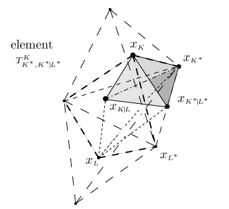
Figure 1. One of the twelve elements in diamond ${\scriptstyle D}^{{{\scriptscriptstyle K}{{\scriptscriptstyle\!|\!}}{\scriptscriptstyle L}}}$ with                   triangular base ${{\scriptstyle K}{\!|\!}{\scriptstyle L}}$

$\bullet$ Define the volume ${\scriptstyle K^{*}}$ associated with a vertex ${x_{\scriptscriptstyle K^{*}}}$ of ${\boldsymbol{\mathfrak{M}}^{o}_{{\Omega}}}$ as the union of all elements ${\scriptstyle T}\in{\mathcal{T}}$ having ${x_{\scriptscriptstyle K^{*}}}$ for one of its vertices. The collection $\overline{{\boldsymbol{\mathfrak{M}}^{*}}}$ of all such ${\scriptstyle K^{*}}$ forms another partition of ${\Omega}$. If ${x_{\scriptscriptstyle K^{*}}}\in{\Omega}\cup\Gamma_{N}$, we say that ${\scriptstyle K^{*}}$ is an (interior) dual control volume and write ${\scriptstyle K^{*}}\in{\boldsymbol{\mathfrak{M}}^{*}}$; and if ${x_{\scriptscriptstyle K^{*}}}\in{\Gamma_{D}}$, we say that ${\scriptstyle K^{*}}$ is a boundary dual control volume and write ${\scriptstyle K^{*}}\in{\partial}{\boldsymbol{\mathfrak{M}}^{*}}$. Thus $\overline{{\boldsymbol{\mathfrak{M}}^{*}}}={\boldsymbol{\mathfrak{M}}^{*}}\cup{\partial}{\boldsymbol{\mathfrak{M}}^{*}}$. Any vertex of any dual control volume ${\scriptstyle K^{*}}\in\overline{{\boldsymbol{\mathfrak{M}}^{*}}}$ is called a dual vertex (of $\overline{{\boldsymbol{\mathfrak{M}}^{*}}}$). Note that by construction, the set of vertices coincides with the set of dual centres ${x_{\scriptscriptstyle K^{*}}}$; the set of dual vertices consists of centres ${x_{\scriptscriptstyle K}}$, face centres $x_{{\scriptscriptstyle K}{{\scriptscriptstyle\!|\!}}{\scriptscriptstyle L}}$ and edge centres (middle points) ${x_{{\scriptscriptstyle K^{*}}{{\scriptscriptstyle\!|\!}}{\scriptscriptstyle L^{*}}}}$. Picturing dual volumes in 3D is a hard task; cf. [49] for version $(A)$ and [21] for version $(C)$.

$\bullet$ We denote by ${{\scriptstyle\mathcal{N}}^{*}}({\scriptstyle K^{*}})$ the set of (dual) neighbours of a dual control volume ${\scriptstyle K^{*}}$, and by ${{\scriptstyle K^{*}}{\!|\!}{\scriptstyle L^{*}}}$, the (dual) interface ${\partial}{\scriptstyle K^{*}}\cap{\partial}{\scriptstyle L^{*}}$ between dual neighbours ${\scriptstyle K^{*}}$ and ${\scriptstyle L^{*}}$.

$\bullet$ Finally, we introduce the partitions of ${\Omega}$ into diamonds and subdiamonds. If ${\scriptstyle K},{\scriptstyle L}\in\overline{{\boldsymbol{\mathfrak{M}}^{o}}}$ are neighbours, let $H_{\scriptscriptstyle K}$ be the convex hull of ${x_{\scriptscriptstyle K}}$ and ${{\scriptstyle K}{\!|\!}{\scriptstyle L}}$ and $H_{\scriptscriptstyle L}$ be the convex hull of ${x_{\scriptscriptstyle L}}$ and ${{\scriptstyle K}{\!|\!}{\scriptstyle L}}$. Then the union $H_{\scriptscriptstyle K}\cup H_{\scriptscriptstyle L}$ is called a diamond and is denoted by ${\scriptstyle D}^{{{\scriptscriptstyle K}{{\scriptscriptstyle\!|\!}}{\scriptscriptstyle L}}}$.

If ${\scriptstyle K},{\scriptstyle L}\in\overline{{\boldsymbol{\mathfrak{M}}^{o}}}$ are neighbours, and ${x_{\scriptscriptstyle K^{*}}},{x_{\scriptscriptstyle L^{*}}}$ are neighbour vertices of the corresponding interface ${{\scriptstyle K}{\!|\!}{\scriptstyle L}}$, then the union of the four elements $\scriptstyle T^{{\scriptscriptstyle K}}_{{\scriptscriptstyle K^{*}},{{\scriptscriptstyle K^{*}}{{\scriptscriptstyle\!|\!}}{\scriptscriptstyle L^{*}}}}$, $\scriptstyle T^{{\scriptscriptstyle K}}_{{\scriptscriptstyle L^{*}},{{\scriptscriptstyle K^{*}}{{\scriptscriptstyle\!|\!}}{\scriptscriptstyle L^{*}}}}$, $\scriptstyle T^{{\scriptscriptstyle L}}_{{\scriptscriptstyle K^{*}},{{\scriptscriptstyle K^{*}}{{\scriptscriptstyle\!|\!}}{\scriptscriptstyle L^{*}}}}$, and $\scriptstyle T^{{\scriptscriptstyle L}}_{{\scriptscriptstyle L^{*}},{{\scriptscriptstyle K^{*}}{{\scriptscriptstyle\!|\!}}{\scriptscriptstyle L^{*}}}}$ is called subdiamond and denoted by ${\scriptstyle S}^{{\scriptscriptstyle K}{{\scriptscriptstyle\!|\!}}{\scriptscriptstyle L}}_{{\scriptscriptstyle K^{*}}{{\scriptscriptstyle\!|\!}}{\scriptscriptstyle L^{*}}}$. In this way, each diamond ${\scriptstyle D}^{{\scriptscriptstyle K}{{\scriptscriptstyle\!|\!}}{\scriptscriptstyle L}}$ gives rise to $l$ subdiamonds (where $l$ is the number of vertices of ${{\scriptstyle K}{\!|\!}{\scriptstyle L}}$); cf. the next item and Fig. 2. Each subdiamond is associated with a unique interface ${{\scriptstyle K}{\!|\!}{\scriptstyle L}}$, and thus with a unique diamond ${\scriptstyle D}^{{\scriptscriptstyle K}{{\scriptscriptstyle\!|\!}}{\scriptscriptstyle L}}$. We will write ${\scriptstyle S}\subset{\scriptstyle D}$ to signify that ${\scriptstyle S}$ is associated with ${\scriptstyle D}$.

We denote by ${\boldsymbol{\mathfrak{D}}}$,${\boldsymbol{\mathfrak{S}}}$ the sets of all diamonds and the set of all subdiamonds, respectively. Generic elements of ${\boldsymbol{\mathfrak{D}}}$,${\boldsymbol{\mathfrak{S}}}$ are denoted by ${\scriptstyle D}$,${\scriptstyle S}$, respectively. Notice that ${\boldsymbol{\mathfrak{D}}}$ is a partition of a subdomain of $\Omega$ (only a small neighbourhood of $\Gamma_{N}$ in ${\Omega}$ is not covered by diamonds).

Figure 2. Primal volumes, diamond; subdiamond and zoom on it                (Version $\!(B)$ of 3D DDFV mesh)

$\bullet$ (See Figure 2) The following notations are only needed for an explicit expression of the discrete divergence operator (and also for the proof of the discrete duality given in [2]). It is convenient to orient the axis ${x_{\scriptscriptstyle K}}{x_{\scriptscriptstyle L}}$ of each diamond ${\scriptstyle D}$. Whenever the orientation is of importance, the primal vertices defining the diamond will be denoted by ${x_{{\scriptscriptstyle K}_{\!\scriptscriptstyle\odot}}},{x_{{\scriptscriptstyle K}_{\!\scriptscriptstyle\oplus}}}$ in such a way that the vector $\overrightarrow{{x_{{\scriptscriptstyle K}_{\!\scriptscriptstyle\odot}}}{x_{{\scriptscriptstyle K}_{\!\scriptscriptstyle\oplus}}}}$ has the positive orientation. The oriented diamond is then denoted by ${\scriptstyle D}^{{{\scriptscriptstyle K}_{\!\scriptscriptstyle\odot}{{\scriptscriptstyle\!|\!}}{\scriptscriptstyle K}_{\!\scriptscriptstyle\oplus}}}$. We denote by ${\vec{e}_{{\scriptscriptstyle K}_{\!\scriptscriptstyle\odot}\!,{\scriptscriptstyle K}_{\!\scriptscriptstyle\oplus}}}$ the corresponding unit vector, and by ${d_{{\scriptscriptstyle K}_{\!\scriptscriptstyle\odot},{\scriptscriptstyle K}_{\!\scriptscriptstyle\oplus}}}$, the length of $\overrightarrow{{x_{{\scriptscriptstyle K}_{\!\scriptscriptstyle\odot}}}{x_{{\scriptscriptstyle K}_{\!\scriptscriptstyle\oplus}}}}$. We denote by ${\vec{n}_{{\scriptscriptstyle K}_{\!\scriptscriptstyle\odot}{{\scriptscriptstyle\!|\!}}{\scriptscriptstyle K}_{\!\scriptscriptstyle\oplus}}}$ the unit normal vector to ${{\scriptstyle K}_{\!\scriptscriptstyle\odot}{\!|\!}{\scriptstyle K}_{\!\scriptscriptstyle\oplus}}$ such that ${\vec{n}_{{\scriptscriptstyle K}_{\!\scriptscriptstyle\odot}{{\scriptscriptstyle\!|\!}}{\scriptscriptstyle K}_{\!\scriptscriptstyle\oplus}}}\cdot{\vec{e}_{{\scriptscriptstyle K}_{\!\scriptscriptstyle\odot}\!,{\scriptscriptstyle K}_{\!\scriptscriptstyle\oplus}}}>0$.

Fixing the normal ${\vec{n}_{{\scriptscriptstyle K}_{\!\scriptscriptstyle\odot}{{\scriptscriptstyle\!|\!}}{\scriptscriptstyle K}_{\!\scriptscriptstyle\oplus}}}$ of ${{\scriptstyle K}_{\!\scriptscriptstyle\odot}{\!|\!}{\scriptstyle K}_{\!\scriptscriptstyle\oplus}}$ induces an orientation of the corresponding face ${{\scriptstyle K}_{\!\scriptscriptstyle\odot}{\!|\!}{\scriptstyle K}_{\!\scriptscriptstyle\oplus}}$, which is a convex polygon with $l$ vertices (we only use $l=3$ or $4$): we denote the vertices of ${{\scriptstyle K}_{\!\scriptscriptstyle\odot}{\!|\!}{\scriptstyle K}_{\!\scriptscriptstyle\oplus}}$ by ${x_{{\scriptscriptstyle K}^{\!*}_{\!i}}}$, $i\in[\![1,l]\!]$, enumerated in the direct sense. By convention, we assign $x_{{\scriptscriptstyle K}^{\!*}_{\!l\!+\!1}}:=x_{{\scriptscriptstyle K}^{\!*}_{1}}$. We denote by ${\vec{e}_{{\scriptscriptstyle K}^{\!*}_{\!i},{\scriptscriptstyle K}^{\!*}_{\!i+\!1}}}$ the unit normal vector pointing from ${x_{{\scriptscriptstyle K}^{\!*}_{\!i}}}$ towards ${x_{{\scriptscriptstyle K}^{\!*}_{\!i+\!1}}}$, and by ${d_{{\scriptscriptstyle K}^{\!*}_{\!i},{\scriptscriptstyle K}^{\!*}_{\!i+\!1}}}$, the length of $\overrightarrow{{x_{{\scriptscriptstyle K}^{\!*}_{\!i}}}{x_{{\scriptscriptstyle K}^{\!*}_{\!i+\!1}}}}$.

To simplify the notation, we will drop the ${\scriptstyle K}$’s in the subscripts and denote the objects introduced above by ${x_{{\!\scriptscriptstyle\odot}}}$,${x_{{\!\scriptscriptstyle\oplus}}}$,${\vec{e}_{\!\scriptscriptstyle\odot,\oplus}}$,${d_{\scriptscriptstyle\odot,\oplus}}$,${\vec{n}_{\!\scriptscriptstyle\odot,\oplus}}$ and by $x^{*}_{i}$,${\vec{e}^{\,*}_{\!i,i+\!1}}$,${d^{*}_{\!i,i+\!1}}$ whenever ${\scriptstyle D}^{{{\scriptscriptstyle K}_{\!\scriptscriptstyle\odot}{{\scriptscriptstyle\!|\!}}{\scriptscriptstyle K}_{\!\scriptscriptstyle\oplus}}}$ is fixed. We also denote by ${x^{*}_{i,i{\scriptscriptstyle+}\!{\scriptscriptstyle 1}}}$ the middle-point $x_{{{\scriptscriptstyle K}^{\!*}_{\!i}{{\scriptscriptstyle\!|\!}}{\scriptscriptstyle K}^{\!*}_{\!i+\!1}}}$ of the segment $[x_{i},x_{\!i+\!1}]$, and by ${x^{*}_{\!\scriptscriptstyle\odot\!,\!\oplus}}$, the centre $x_{{\scriptscriptstyle K}_{\!\scriptscriptstyle\odot}{{\scriptscriptstyle\!|\!}}{\scriptscriptstyle K}_{\!\scriptscriptstyle\oplus}}$ of ${{\scriptstyle K}_{\!\scriptscriptstyle\odot}{\!|\!}{\scriptstyle K}_{\!\scriptscriptstyle\oplus}}$.

$\bullet$ For a diamond ${\scriptstyle D}={\scriptstyle D}^{{{\scriptscriptstyle K}_{\!\scriptscriptstyle\odot}{{\scriptscriptstyle\!|\!}}{\scriptscriptstyle K}_{\!\scriptscriptstyle\oplus}}}$, we denote by ${\text{Proj}_{\scriptscriptstyle D}}$ the orthogonal projection of ${\mathbb{R}}^{3}$ onto the line spanned by the vector ${\vec{e}_{{\scriptscriptstyle K}_{\!\scriptscriptstyle\odot}\!,{\scriptscriptstyle K}_{\!\scriptscriptstyle\oplus}}}$; we denote by ${\text{Proj}^{*}_{\scriptscriptstyle D}}$ the orthogonal projection of ${\mathbb{R}}^{3}$ onto the plane containing the interface ${{\scriptstyle K}_{\!\scriptscriptstyle\odot}{\!|\!}{\scriptstyle K}_{\!\scriptscriptstyle\oplus}}$.

$\bullet$ We denote by ${\text{\footnotesize\sl Vol}}(A)$ the three-dimensional Lebesgue measure of $A$ which can stand for a control volume, a dual control volume, or a diamond. In particular, for ${\scriptstyle K}\in{\boldsymbol{\mathfrak{M}}^{o}_{\Gamma_{N}}}$, ${\text{\footnotesize\sl Vol}}({\scriptstyle K})=0$: these volumes are degenerate. For a subdiamond ${\scriptstyle S}={\scriptstyle S}^{{{\scriptscriptstyle K}_{\!\scriptscriptstyle\odot}{{\scriptscriptstyle\!|\!}}{\scriptscriptstyle K}_{\!\scriptscriptstyle\oplus}}}_{{{{\scriptscriptstyle K}^{\!*}_{\!i}{{\scriptscriptstyle\!|\!}}{\scriptscriptstyle K}^{\!*}_{\!i+\!1}}}}$, we have the formula ${\text{\footnotesize\sl Vol}}({\scriptstyle S})=\frac{1}{6}\,\langle\,\overrightarrow{{x_{{\!\scriptscriptstyle\odot}}}{x_{{\!\scriptscriptstyle\oplus}}}},\overrightarrow{{x^{*}_{\!\scriptscriptstyle\odot\!,\!\oplus}}{x^{*}_{i,i{\scriptscriptstyle+}\!{\scriptscriptstyle 1}}}},\overrightarrow{x^{*}_{i}x^{*}_{i+\!1}}\,\rangle$. Note the mixed product is positive, thanks to our conventions on the orientation in ${\scriptstyle D}^{{\scriptscriptstyle K}_{\!\scriptscriptstyle\odot}{{\scriptscriptstyle\!|\!}}{\scriptscriptstyle K}_{\!\scriptscriptstyle\oplus}}$ and because we have assumed that ${x^{*}_{\!\scriptscriptstyle\odot\!,\!\oplus}}\in{{\scriptstyle K}_{\!\scriptscriptstyle\odot}{\!|\!}{\scriptstyle K}_{\!\scriptscriptstyle\oplus}}$.

Remark 3.1.

Diamonds permit to define the discrete gradient operator, while subdiamonds permit to give formulas for the discrete divergence operator (see (13), (14) and (17), (21) below, respectively).

In the context of $2D$ “double” schemes, introducing diamonds is quite standard (see, e.g., [6, 26]). Subdiamonds are “hidden” in the $2D$ construction : they actually coincide with diamonds.

3.2.2. Discrete functions, fields, and boundary data.

$\bullet$ A discrete function $w^{\scriptscriptstyle\boldsymbol{\mathfrak{T}}}$ on ${{\Omega}}$ is a pair $\Bigl{(}{w^{\scriptscriptstyle\boldsymbol{\mathfrak{M}}^{o}}},{w^{\scriptscriptstyle\boldsymbol{\mathfrak{M}}^{*}}}\Bigr{)}$ consisting of two sets of real values $w^{\scriptscriptstyle\boldsymbol{\mathfrak{M}}^{o}}=(w_{\scriptscriptstyle K})_{{\scriptscriptstyle K}\in{\scriptscriptstyle\boldsymbol{\mathfrak{M}}^{o}}}$ and $w^{\scriptscriptstyle\boldsymbol{\mathfrak{M}}^{*}}=(w_{\scriptscriptstyle K^{*}})_{{\scriptscriptstyle K^{*}}\in{\scriptscriptstyle\boldsymbol{\mathfrak{M}}^{*}}}$. The set of all such functions is denoted by ${\mathbb{R}}^{\scriptscriptstyle\boldsymbol{\mathfrak{T}}}$.

$\bullet$ A discrete field $\vec{\mathcal{M}}^{\scriptscriptstyle\boldsymbol{\mathfrak{T}}}$ on ${\Omega}$ is a set $\Bigl{(}\vec{\mathcal{F}}_{\scriptscriptstyle D}\Bigr{)}_{{\scriptscriptstyle D}\in{\scriptscriptstyle\boldsymbol{\mathfrak{D}}}}$ of vectors of ${\mathbb{R}}^{d}$. The set of all discrete fields is denoted by $({\mathbb{R}}^{d})^{\scriptscriptstyle\boldsymbol{\mathfrak{D}}}$. If $\vec{\mathcal{M}}^{\scriptscriptstyle\boldsymbol{\mathfrak{T}}}$ is a discrete field on ${\Omega}$, we assign $\vec{\mathcal{M}}_{\scriptscriptstyle S}=\vec{\mathcal{M}}_{\scriptscriptstyle D}$ whenever ${\scriptstyle S}\subset{\scriptstyle D}$.

$\bullet$ A discrete Dirichlet datum $g^{\scriptscriptstyle\boldsymbol{\mathfrak{T}}}$ on $\Gamma_{D}$ is a pair $\Bigl{(}g^{{\scriptscriptstyle{\partial}}{\scriptscriptstyle\boldsymbol{\mathfrak{M}}^{o}}},g^{{\scriptscriptstyle{\partial}}{\scriptscriptstyle\boldsymbol{\mathfrak{M}}^{*}}}\Bigr{)}$ consisting of two sets of real values $g^{{\scriptscriptstyle{\partial}}{\scriptscriptstyle\boldsymbol{\mathfrak{M}}^{o}}}=(g_{\scriptscriptstyle K})_{{\scriptscriptstyle K}\in{\scriptscriptstyle{\partial}}{\scriptscriptstyle\boldsymbol{\mathfrak{M}}^{o}}}$ and $g^{{\scriptscriptstyle{\partial}}{\scriptscriptstyle\boldsymbol{\mathfrak{M}}^{*}}}=(g_{\scriptscriptstyle K^{*}})_{{\scriptscriptstyle K^{*}}\in{\scriptscriptstyle{\partial}}{\scriptscriptstyle\boldsymbol{\mathfrak{M}}^{*}}}$. In practise, $g_{\scriptstyle K}$ (resp., $g_{\scriptstyle K^{*}}$) can be obtained by averaging the “continuous” Dirichlet datum $g$ over the boundary volume ${\scriptstyle K}\subset\Gamma_{D}$ (resp., over the part of $\Gamma_{D}$ adjacent to the boundary dual volume ${\scriptstyle K^{*}}$); if $g$ is continuous, the mean value can be replaced by the value of $g$ at ${x_{\scriptscriptstyle K}}$ (resp., at ${x_{\scriptscriptstyle K^{*}}}$). We refer to [6] for details.

$\bullet$ A discrete Neumann datum $s^{{\scriptscriptstyle\boldsymbol{\mathfrak{T}}}}$ on $\Gamma_{N}$ is a set of real values $(s_{\scriptscriptstyle K})_{{\scriptscriptstyle K}\in{\scriptscriptstyle\boldsymbol{\mathfrak{M}}^{o}_{\Gamma_{N}}}}$.

In practice, $s_{\scriptscriptstyle K}$ can be obtained by averaging the “continuous” Neumann datum $s$ over the degenerate volume ${\scriptstyle K}\subset\Gamma_{N}$. In the case $\Gamma_{D}=\text{\O}$, one should be careful while using approximate quadratures to produce $s^{\scriptscriptstyle\boldsymbol{\mathfrak{T}}}$ from $s$. Indeed, some compatibility conditions between Neumann data and source terms may arise while discretising elliptic equations (this is the case of system (1), because the difference of the two equations of the system is an elliptic equation, and the compatibility condition (5) is needed for the solvability of the system). The compatibility condition, expressed in terms of $\int_{\Gamma_{N}}s_{i,e}$, should be preserved at the discrete level. This is the case for the above choice of $s^{\scriptscriptstyle\boldsymbol{\mathfrak{T}}}$: indeed, we have the equality $\int_{\Gamma_{N}}s=\int_{\Gamma_{N}}s^{\scriptscriptstyle\boldsymbol{\mathfrak{T}}}$.

3.2.3. The discrete gradient operator

$\bullet$ On the set ${\mathbb{R}}^{\scriptscriptstyle\boldsymbol{\mathfrak{T}}}$ of discrete functions $w^{\scriptscriptstyle\boldsymbol{\mathfrak{T}}}$ on ${{\Omega}}$, we define the discrete gradient operator ${\,\nabla}_{g^{\scriptscriptstyle\boldsymbol{\mathfrak{T}}}}^{\scriptscriptstyle\boldsymbol{\mathfrak{T}}}[\cdot]$ with Dirichlet data $g^{\scriptscriptstyle\boldsymbol{\mathfrak{T}}}$ on $\Gamma_{D}$:

(13) $${\,\nabla}_{g^{\scriptscriptstyle\boldsymbol{\mathfrak{T}}}}^{\scriptscriptstyle\boldsymbol{\mathfrak{T}}}:w^{\scriptscriptstyle\boldsymbol{\mathfrak{T}}}\in{\mathbb{R}}^{\scriptscriptstyle\boldsymbol{\mathfrak{T}}}\mapsto{\,\nabla}_{g^{\scriptscriptstyle\boldsymbol{\mathfrak{T}}}}^{\scriptscriptstyle\boldsymbol{\mathfrak{T}}}w^{\scriptscriptstyle\boldsymbol{\mathfrak{T}}}=\Bigl{(}{\,\nabla}_{\scriptscriptstyle D}w^{\scriptscriptstyle\boldsymbol{\mathfrak{T}}}\Bigr{)}_{{\scriptscriptstyle D}\in{\scriptscriptstyle\boldsymbol{\mathfrak{D}}}}\in({\mathbb{R}}^{d})^{\scriptscriptstyle\boldsymbol{\mathfrak{D}}},$$

where the entry ${\,\nabla}_{\!{\scriptscriptstyle D}}w^{\scriptscriptstyle\boldsymbol{\mathfrak{T}}}$ of the discrete field ${\,\nabla}^{\scriptscriptstyle\boldsymbol{\mathfrak{T}}}w^{\scriptscriptstyle\boldsymbol{\mathfrak{T}}}$ relative to ${\scriptstyle D}={\scriptstyle D}^{{{\scriptscriptstyle K}_{\!\scriptscriptstyle\odot}{{\scriptscriptstyle\!|\!}}{\scriptscriptstyle K}_{\!\scriptscriptstyle\oplus}}}$ is

(14) $$\text{${\,\nabla}_{\!{\scriptscriptstyle D}}w^{\scriptscriptstyle\boldsymbol{\mathfrak{T}}}$ is s.t. }\left\{\begin{array}[]{l}\displaystyle{\text{Proj}_{\scriptscriptstyle D}}({\,\nabla}_{\!{\scriptscriptstyle D}}w^{\scriptscriptstyle\boldsymbol{\mathfrak{T}}})=\frac{{w_{\!\scriptscriptstyle\oplus}}-{w_{\!\scriptscriptstyle\odot}}}{{d_{\scriptscriptstyle\odot,\oplus}}}\,{\vec{e}_{\!\scriptscriptstyle\odot,\oplus}},\\[8.0pt] \displaystyle{\text{Proj}^{*}_{\scriptscriptstyle D}}({\,\nabla}_{\!{\scriptscriptstyle D}}w^{\scriptscriptstyle\boldsymbol{\mathfrak{T}}})={\,\nabla}F(\cdot),\end{array}\right.$$

where

• $F(\cdot)$ is the affine function from ${\mathbb{R}}^{3}$ to ${\mathbb{R}}$ that is constant in the direction ${\vec{n}_{\!\scriptscriptstyle\odot,\oplus}}$ orthogonal to ${{\scriptstyle K}{\!|\!}{\scriptstyle L}}$ and that is the ad hoc affine interpolation (namely, (15) below) of the values $w^{*}_{i}$ at the vertices $x^{*}_{i}$, $i=1,\ldots,l$, of ${{\scriptstyle K}{\!|\!}{\scriptstyle L}}$;

• for the vertices of ${\scriptstyle D}$ lying in ${\Omega}\cup\Gamma_{N}$, ${w_{\!\scriptscriptstyle\odot}}\!=\!w_{{\scriptscriptstyle K}_{\!\scriptscriptstyle\odot}},\,{w_{\!\scriptscriptstyle\oplus}}\!=\!w_{{\scriptscriptstyle K}_{\!\scriptscriptstyle\oplus}}$, $w^{*}_{i}=w_{{\scriptscriptstyle K}^{\!*}_{\!i}}$, etc. (we use the simplified notation in the diamond ${\scriptstyle D}={\scriptstyle D}^{{{\scriptscriptstyle K}_{\!\scriptscriptstyle\odot}{{\scriptscriptstyle\!|\!}}{\scriptscriptstyle K}_{\!\scriptscriptstyle\oplus}}}$, as depicted in Figure 2). For the vertices of ${\scriptstyle D}$ that lie in $\Gamma_{D}$, the values of $g^{\scriptscriptstyle\boldsymbol{\mathfrak{T}}}$ are used: e.g., if $x_{{\scriptscriptstyle K}_{\!\scriptscriptstyle\odot}}\in\Gamma_{D}$, then we set ${w_{\!\scriptscriptstyle\odot}}:=g_{{\scriptscriptstyle K}_{\!\scriptscriptstyle\odot}}$ in the above formula.

Clearly, if $l=3$ there is a unique consistent interpolation of the values $w_{1},w_{2},w_{3}$. For $l\geq 4$, no consistent interpolation exists, and we choose the linear form in $w^{*}_{\!i}$ that leads to the expression

(15) $${\text{Proj}^{*}_{\scriptscriptstyle D}}({\,\nabla}_{\!{\scriptscriptstyle D}}w^{\scriptscriptstyle\boldsymbol{\mathfrak{T}}})\!=\!\frac{2}{\sum_{i=1}^{l}\,\langle\,{\vec{n}_{\!\scriptscriptstyle\odot,\oplus}},\overrightarrow{{x^{*}_{\!\scriptscriptstyle\odot\!,\!\oplus}}{x^{*}_{i,i{\scriptscriptstyle+}\!{\scriptscriptstyle 1}}}},\overrightarrow{x^{*}_{i}x^{*}_{i+\!1}}\,\rangle}\;\sum_{i=1}^{l}(w^{*}_{\!i+\!1}-w^{*}_{\!i})\;\Bigl{[}{\vec{n}_{\!\scriptscriptstyle\odot,\oplus}}\times\overrightarrow{{x^{*}_{\!\scriptscriptstyle\odot\!,\!\oplus}}{x^{*}_{i,i{\scriptscriptstyle+}\!{\scriptscriptstyle 1}}}}\Bigr{]};$$

it is shown in [2] that this choice is exact on affine functions, and that it leads to the discrete duality formula. For an explicit formula of ${\,\nabla}_{\!{\scriptscriptstyle D}}w^{\scriptscriptstyle\boldsymbol{\mathfrak{T}}}$, note that $\vec{p}={\text{Proj}_{\scriptscriptstyle D}}({\,\nabla}_{\!{\scriptscriptstyle D}}w^{\scriptscriptstyle\boldsymbol{\mathfrak{T}}})$, $\vec{p^{*}}={\text{Proj}^{*}_{\scriptscriptstyle D}}({\,\nabla}_{\!{\scriptscriptstyle D}}w^{\scriptscriptstyle\boldsymbol{\mathfrak{T}}})$ are given; then one expresses ${\,\nabla}_{\!{\scriptscriptstyle D}}w^{\scriptscriptstyle\boldsymbol{\mathfrak{T}}}$ as

(16) $${\,\nabla}_{\!{\scriptscriptstyle D}}w^{\overline{{\scriptscriptstyle\boldsymbol{\mathfrak{T}}}}}=\frac{1}{{\text{\footnotesize\sl Vol}}({\scriptstyle D})}\sum_{i=1}^{l}\biggl{\{}\frac{{\text{\footnotesize\sl Vol}}({\scriptstyle S}^{{{\scriptscriptstyle K}_{\!\scriptscriptstyle\odot}{{\scriptscriptstyle\!|\!}}{\scriptscriptstyle K}_{\!\scriptscriptstyle\oplus}}}_{{{{\scriptscriptstyle K}^{\!*}_{\!i}{{\scriptscriptstyle\!|\!}}{\scriptscriptstyle K}^{\!*}_{\!i+\!1}}}})}{\overrightarrow{{x_{{\!\scriptscriptstyle\odot}}}{x_{{\!\scriptscriptstyle\oplus}}}}\cdot{\vec{n}_{\!\scriptscriptstyle\odot,\oplus}}}({w_{\!\scriptscriptstyle\oplus}}-{w_{\!\scriptscriptstyle\odot}})\,{\vec{n}_{\!\scriptscriptstyle\odot,\oplus}}+\frac{1}{3}(w^{*}_{\!i+\!1}-w^{*}_{\!i})\;\Bigl{[}\overrightarrow{{x_{{\!\scriptscriptstyle\odot}}}{x_{{\!\scriptscriptstyle\oplus}}}}\times\overrightarrow{{x^{*}_{\!\scriptscriptstyle\odot\!,\!\oplus}}{x^{*}_{i,i{\scriptscriptstyle+}\!{\scriptscriptstyle 1}}}}\Bigr{]}\biggr{\}}$$

Remark 3.2.

In (14), the primal mesh $\overline{{\boldsymbol{\mathfrak{M}}^{o}}}$ serves to reconstruct one component of the gradient, which is the one in the direction ${\vec{e}_{\!\scriptscriptstyle\odot,\oplus}}$. The dual mesh $\overline{{\boldsymbol{\mathfrak{M}}^{*}}}$ serves to reconstruct, with the help of the formula (15), the two other components, which are those lying in the plane containing ${{\scriptstyle K}_{\!\scriptscriptstyle\odot}{\!|\!}{\scriptstyle K}_{\!\scriptscriptstyle\oplus}}$. The same happens for version $(A)$ of the scheme. On the contrary, version $(C)$ only reconstructs one direction of the discrete gradient on the mesh ${\boldsymbol{\mathfrak{M}}^{*}}$, while the third direction is reconstructed on a third mesh that we denote by ${\boldsymbol{\mathfrak{M}}^{\scriptstyle\diamond}}$.

Remark 3.3.

We stress that our gradient approximation is consistent (see [2] for the proof). Indeed, let ${w_{\!\scriptscriptstyle\odot}},{w_{\!\scriptscriptstyle\oplus}},(w^{*}_{i,i+\!1})_{i=1}^{l}$ be the values at the points ${x_{{\!\scriptscriptstyle\odot}}},{x_{{\!\scriptscriptstyle\oplus}}},({x^{*}_{i,i{\scriptscriptstyle+}\!{\scriptscriptstyle 1}}})_{i=1}^{l}$, respectively, of an affine on ${\scriptstyle D}={\scriptstyle D}^{{\scriptscriptstyle K}_{\!\scriptscriptstyle\odot}{{\scriptscriptstyle\!|\!}}{\scriptscriptstyle K}_{\!\scriptscriptstyle\oplus}}$ function $w$. Then ${\,\nabla}_{\scriptscriptstyle D}w^{\scriptscriptstyle\boldsymbol{\mathfrak{T}}}$ coincides with the value of ${\,\nabla}w$ on ${\scriptstyle D}$.

3.2.4. The discrete divergence operator

$\bullet$ On the set $({\mathbb{R}}^{d})^{\scriptscriptstyle\boldsymbol{\mathfrak{D}}}$ of discrete fields $\vec{\mathcal{M}}^{\scriptscriptstyle\boldsymbol{\mathfrak{T}}}$, we define the discrete divergence operator ${\rm div\,}_{\!\!s^{\scriptscriptstyle\boldsymbol{\mathfrak{T}}}}^{\!\!{\scriptscriptstyle\boldsymbol{\mathfrak{T}}}}[\cdot]$ with Neumann data $s^{\scriptscriptstyle\boldsymbol{\mathfrak{T}}}$ on $\Gamma_{N}$:

(17) $$\begin{split}{\rm div\,}_{\!\!s^{\scriptscriptstyle\boldsymbol{\mathfrak{T}}}}^{\!\!{\scriptscriptstyle\boldsymbol{\mathfrak{T}}}}:\vec{\mathcal{M}}^{\scriptscriptstyle\boldsymbol{\mathfrak{T}}}\in({\mathbb{R}}^{d})^{\scriptscriptstyle\boldsymbol{\mathfrak{D}}}&\mapsto{\rm div\,}_{\!\!s^{\scriptscriptstyle\boldsymbol{\mathfrak{T}}}}^{\!\!{\scriptscriptstyle\boldsymbol{\mathfrak{T}}}}\vec{\mathcal{M}}^{\scriptscriptstyle\boldsymbol{\mathfrak{T}}}\\ &=\biggl{(}\,\Bigl{(}{\rm div\,}_{\!\!{\scriptscriptstyle K}}\vec{\mathcal{M}}^{\scriptscriptstyle\boldsymbol{\mathfrak{T}}}\Bigr{)}_{{\scriptscriptstyle K}\in{\scriptscriptstyle\boldsymbol{\mathfrak{M}}^{o}}={\scriptscriptstyle\boldsymbol{\mathfrak{M}}^{o}_{{\Omega}}}\cup{\scriptscriptstyle\boldsymbol{\mathfrak{M}}^{o}_{\Gamma_{N}}}}\,,\,\Bigl{(}{\rm div\,}_{\!\!{\scriptscriptstyle K^{*}}}\vec{\mathcal{M}}^{\scriptscriptstyle\boldsymbol{\mathfrak{T}}}\Bigr{)}_{{\scriptscriptstyle K^{*}}\in{\scriptscriptstyle\boldsymbol{\mathfrak{M}}^{*}}}\,\biggr{)}\in{\mathbb{R}}^{\scriptscriptstyle\boldsymbol{\mathfrak{T}}},\end{split}$$

where the entries ${\rm div\,}_{\!\!{\scriptscriptstyle K}}\vec{\mathcal{M}}^{\scriptscriptstyle\boldsymbol{\mathfrak{T}}}$ (for ${\scriptstyle K}\in{\boldsymbol{\mathfrak{M}}^{o}_{{\Omega}}}$) and ${\rm div\,}_{\!\!{\scriptscriptstyle K^{*}}}\vec{\mathcal{M}}^{\scriptscriptstyle\boldsymbol{\mathfrak{T}}}$ of the discrete function ${\rm div\,}^{\!\!{\scriptscriptstyle\boldsymbol{\mathfrak{T}}}}\vec{\mathcal{M}}^{\scriptscriptstyle\boldsymbol{\mathfrak{T}}}$ on ${\Omega}$ are given by

(18) $$\begin{array}[]{l}\displaystyle\forall\,{\scriptstyle K}\in{\boldsymbol{\mathfrak{M}}^{o}_{{\Omega}}},\;\;{\rm div\,}_{\!\!{\scriptscriptstyle K}}\vec{\mathcal{M}}^{\scriptscriptstyle\boldsymbol{\mathfrak{T}}}=\frac{1}{{\text{\footnotesize\sl Vol}}({\scriptscriptstyle K})}\sum_{{\scriptscriptstyle D}\in{\scriptscriptstyle\boldsymbol{\mathfrak{D}}}:\,{\scriptscriptstyle D}\cap{\scriptscriptstyle K}\neq\text{\O}}\int_{{\scriptscriptstyle{\partial}}{\scriptscriptstyle K}\cap{\scriptscriptstyle D}}\vec{\mathcal{M}}_{D}\cdot n_{\scriptscriptstyle K},\\[7.0pt] \displaystyle\forall\,{\scriptstyle K^{*}}\in{\boldsymbol{\mathfrak{M}}^{*}},\;\;{\rm div\,}_{\!\!{\scriptscriptstyle K^{*}}}\vec{\mathcal{M}}^{\scriptscriptstyle\boldsymbol{\mathfrak{T}}}=\frac{1}{{\text{\footnotesize\sl Vol}}({\scriptscriptstyle K^{*}})}\sum_{{\scriptscriptstyle D}\in{\scriptscriptstyle\boldsymbol{\mathfrak{D}}}:\,{\scriptscriptstyle D}\cap{\scriptscriptstyle K^{*}}\neq\text{\O}}\int_{{\scriptscriptstyle{\partial}}{\scriptscriptstyle K^{*}}\cap{\scriptscriptstyle D}}\vec{\mathcal{M}}_{D}\cdot n_{\scriptscriptstyle K^{*}},\end{array}$$

where $n_{\scriptscriptstyle K}$ (resp., $n_{\scriptscriptstyle K^{*}}$) denotes the exterior unit normal vector to ${\scriptstyle K}$ (resp., to ${\scriptstyle K^{*}}$). Further, for ${\scriptstyle K}\in{\boldsymbol{\mathfrak{M}}^{o}_{\Gamma_{N}}}$, we mean that $n_{\scriptscriptstyle K}$ points inside ${\Omega}$, and we adapt the following formal definition:

(19) $$\begin{array}[]{l}\displaystyle\forall\,{\scriptstyle K}\in{\boldsymbol{\mathfrak{M}}^{o}_{\Gamma_{N}}},\;\;{{\text{\footnotesize\sl Vol}}({\scriptstyle K})}{\rm div\,}_{\!\!{\scriptscriptstyle K}}\vec{\mathcal{M}}^{\scriptscriptstyle\boldsymbol{\mathfrak{T}}}:=\vec{\mathcal{M}}_{D}\cdot n_{\scriptscriptstyle K}+s_{\scriptscriptstyle K}\\ \displaystyle\text{for the diamond ${\scriptstyle D}$ such that $\overline{{\scriptstyle D}}\cap\Gamma_{N}={\scriptstyle K}$};\end{array}$$

thus, although ${\text{\footnotesize\sl Vol}}({\scriptstyle K})$ is zero, in calculations we only use the products ${\text{\footnotesize\sl Vol}}({\scriptstyle K}){\rm div\,}_{\!\!{\scriptscriptstyle K}}\vec{\mathcal{M}}^{\scriptscriptstyle\boldsymbol{\mathfrak{T}}}$, which are well defined thanks to convention (19). In practise, the discrete equations corresponding to volumes of ${\boldsymbol{\mathfrak{M}}^{o}_{\Gamma_{N}}}$ will always read as

(20) $$\vec{\mathcal{M}}_{D}\cdot n_{\scriptscriptstyle K}+s_{\scriptscriptstyle K}=0,\quad{\scriptstyle K}\in{\boldsymbol{\mathfrak{M}}^{o}_{\Gamma_{N}}}.$$

Notice that the values of the Neumann data $s^{\scriptscriptstyle\boldsymbol{\mathfrak{T}}}$ only appear in the convention (19) for the degenerate primal volumes ${\scriptstyle K}\subset\Gamma_{N}$; at the same time, in the volumes ${\scriptstyle K^{*}}$ adjacent to $\Gamma_{N}$ the data $s^{\scriptscriptstyle\boldsymbol{\mathfrak{T}}}$ are taken into account indirectly. Namely, let ${\scriptstyle K^{*}}$ be a dual volume adjacent to $\Gamma_{N}$, and let ${\scriptstyle D}$ be a diamond intersecting ${\scriptstyle K^{*}}$ and adjacent to $\Gamma_{N}$; then the value ${\mathcal{M}}_{D}\cdot n_{\scriptscriptstyle K}$ used for the definition of ${\rm div\,}_{\!\!{\scriptscriptstyle K^{*}}}\vec{\mathcal{M}}^{\scriptscriptstyle\boldsymbol{\mathfrak{T}}}$ is linked to the data $s^{\scriptscriptstyle\boldsymbol{\mathfrak{T}}}$ via equations (20).

The formulas (18) are standard for divergence discretisation in finite volume methods; their interpretation is straightforward, using the Green-Gauss theorem. The consistency of the discrete divergence operator (in the weak sense) can be inferred by duality from the one of the discrete gradient operator (Remark 3.3) and from the discrete duality property (11); see Proposition 5.1(iii) and [2].

For the explicit calculation of the right-hand sides in (18), one can further split diamonds into subdiamonds. In a generic subdiamond, we use the following notation. Consider ${\scriptstyle S}\in{\boldsymbol{\mathfrak{S}}}$; it is associated with a unique oriented diamond which we denote ${\scriptstyle D}^{{{\scriptscriptstyle K}_{\!\scriptscriptstyle\odot}{{\scriptscriptstyle\!|\!}}{\scriptscriptstyle K}_{\!\scriptscriptstyle\oplus}}}$, so that ${\scriptstyle S}$ is of the form ${\scriptstyle S}={\scriptstyle S}^{{{\scriptscriptstyle K}_{\!\scriptscriptstyle\odot}{{\scriptscriptstyle\!|\!}}{\scriptscriptstyle K}_{\!\scriptscriptstyle\oplus}}}_{{{{\scriptscriptstyle K}^{\!*}_{\!i}{{\scriptscriptstyle\!|\!}}{\scriptscriptstyle K}^{\!*}_{\!i+\!1}}}}$. In order to cope with the vector orientation issues, given ${\scriptstyle S}={\scriptstyle S}^{{{\scriptscriptstyle K}_{\!\scriptscriptstyle\odot}{{\scriptscriptstyle\!|\!}}{\scriptscriptstyle K}_{\!\scriptscriptstyle\oplus}}}_{{{{\scriptscriptstyle K}^{\!*}_{\!i}{{\scriptscriptstyle\!|\!}}{\scriptscriptstyle K}^{\!*}_{\!i+\!1}}}}$ we define

$${\epsilon_{\scriptscriptstyle S}^{\scriptscriptstyle K}}:=\begin{cases}0,\text{ if ${\scriptstyle K}={{\scriptstyle K}_{\!\scriptscriptstyle\odot}}$}\\ 1,\text{ if ${\scriptstyle K}={{\scriptstyle K}_{\!\scriptscriptstyle\oplus}}$}\end{cases},\qquad{\epsilon_{\scriptscriptstyle S}^{\scriptscriptstyle K^{*}}}:=\begin{cases}0,\text{ if ${\scriptstyle K^{*}}={\scriptstyle K}^{*}_{i}$}\\ 1,\text{ if ${\scriptstyle K^{*}}={\scriptstyle K}^{*}_{i+\!1}$}\end{cases}.$$

For ${\scriptstyle K}\in{\boldsymbol{\mathfrak{M}}^{o}}$, we denote by ${\scriptstyle\mathcal{V}}({\scriptstyle K})$ the set of all subdiamonds ${\scriptstyle S}\in{\boldsymbol{\mathfrak{S}}}$ such that ${\scriptstyle K}\cap{\scriptstyle S}\neq\text{\O}$. In the same way, for ${\scriptstyle K^{*}}\in{\boldsymbol{\mathfrak{M}}^{*}}$ we define the set ${{\scriptstyle\mathcal{V}}^{*}}({\scriptstyle K^{*}})$ of the subdiamonds intersecting ${\scriptstyle K^{*}}$. Then, using the notation $\langle\cdot,\cdot,\cdot\rangle$ for the mixed product on ${\mathbb{R}}^{3}$, we can express formulae (18) as

(21) $$\begin{array}[]{l}\displaystyle\forall\,{\scriptstyle K}\in{\boldsymbol{\mathfrak{M}}^{o}_{{\Omega}}}\;\;\;\;{\rm div\,}_{\!\!{\scriptscriptstyle K}}\vec{\mathcal{M}}^{\scriptscriptstyle\boldsymbol{\mathfrak{T}}}=\frac{1}{2{\text{\footnotesize\sl Vol}}({\scriptscriptstyle K})}\!\!\!\!\!\!\sum_{\hskip 8.53581pt{\scriptscriptstyle S}\in{\scriptscriptstyle\mathcal{V}}({\scriptscriptstyle K})}\!\!\!\!(-1)^{\textstyle\epsilon_{\scriptscriptstyle S}^{\scriptscriptstyle K}}\langle\,\vec{\mathcal{M}}_{\!{\scriptscriptstyle S}},\overrightarrow{{x^{*}_{\!\scriptscriptstyle\odot\!,\!\oplus}}{x^{*}_{i,i{\scriptscriptstyle+}\!{\scriptscriptstyle 1}}}},\overrightarrow{x^{*}_{i}x^{*}_{i+\!1}},\,\rangle\\[7.0pt] \displaystyle\forall\,{\scriptstyle K^{*}}\in{\boldsymbol{\mathfrak{M}}^{*}}\;\;\;\;{\rm div\,}_{\!\!{\scriptscriptstyle K^{*}}}\vec{\mathcal{M}}^{\scriptscriptstyle\boldsymbol{\mathfrak{T}}}=\frac{1}{2{\text{\footnotesize\sl Vol}}({\scriptscriptstyle K^{*}})}\!\!\!\!\!\!\!\!\!\!\sum_{\hskip 14.22636pt{\scriptscriptstyle S}\in{{\scriptscriptstyle\mathcal{V}}^{*}}({\scriptscriptstyle K^{*}})}\!\!\!\!\!\!\!\!(-1)^{\textstyle\epsilon_{\scriptscriptstyle S}^{\scriptscriptstyle K^{\!*}}}\!\langle\,\vec{\mathcal{M}}_{\!{\scriptscriptstyle S}},\overrightarrow{{x_{{\!\scriptscriptstyle\odot}}}{x_{{\!\scriptscriptstyle\oplus}}}},\overrightarrow{{x^{*}_{\!\scriptscriptstyle\odot\!,\!\oplus}}{x^{*}_{i,i{\scriptscriptstyle+}\!{\scriptscriptstyle 1}}}}\,\rangle.\end{array}$$

In (21), each subdiamond ${\scriptstyle S}$ in ${\scriptstyle\mathcal{V}}({\scriptstyle K})$ (or in ${{\scriptstyle\mathcal{V}}^{*}}({\scriptstyle K^{*}})$) has the form ${\scriptstyle S}={\scriptstyle S}^{{{\scriptscriptstyle K}_{\!\scriptscriptstyle\odot}{{\scriptscriptstyle\!|\!}}{\scriptscriptstyle K}_{\!\scriptscriptstyle\oplus}}}_{{{{\scriptscriptstyle K}^{\!*}_{\!i}{{\scriptscriptstyle\!|\!}}{\scriptscriptstyle K}^{\!*}_{\!i+\!1}}}}$, with some ${{\scriptstyle K}_{\!\scriptscriptstyle\odot}},{{\scriptstyle K}_{\!\scriptscriptstyle\oplus}},{\scriptstyle K}^{*}_{i},{\scriptstyle K}^{*}_{i+\!1}$; the notations ${\epsilon_{\scriptscriptstyle S}^{\scriptscriptstyle K}},{\epsilon_{\scriptscriptstyle S}^{\scriptscriptstyle K^{*}}},{x_{{\!\scriptscriptstyle\odot}}},{x_{{\!\scriptscriptstyle\oplus}}},{x^{*}_{\!\scriptscriptstyle\odot\!,\!\oplus}},{x^{*}_{i,i{\scriptscriptstyle+}\!{\scriptscriptstyle 1}}},x^{*}_{i},x^{*}_{i+\!1}$ refer to ${\scriptstyle S}={\scriptstyle S}^{{{\scriptscriptstyle K}_{\!\scriptscriptstyle\odot}{{\scriptscriptstyle\!|\!}}{\scriptscriptstyle K}_{\!\scriptscriptstyle\oplus}}}_{{{{\scriptscriptstyle K}^{\!*}_{\!i}{{\scriptscriptstyle\!|\!}}{\scriptscriptstyle K}^{\!*}_{\!i+\!1}}}}$ (see Figure 2). Details can be found in [2].

Remark 3.4.

In practise it is not necessary to calculate the discrete divergence; indeed, with the help of the duality property, one can express the discrete system of equations in the dual form, where the calculation of the discrete divergence of the solution is replaced by the calculation of the discrete gradient of a test function. Thus, as for the so-called mimetic finite difference methods, in order to formulate a DDFV scheme it is sufficient to calculate discrete gradients. This amounts to the “discrete weak formulation” (27) we use in the sequel.

3.2.5. The scalar products ${\biggl{[}\biggl{[}}\cdot,\cdot{\biggr{]}\biggr{]}}_{{\Omega}},{\biggl{\{}\!\!\!\biggl{\{}}\cdot,\cdot{\biggr{\}}\!\!\!\biggr{\}}}_{{\Omega}},{\biggl{<}\biggl{<}}\cdot,\cdot{\biggr{>}\biggr{>}}_{\Gamma_{N}}$ and discrete duality

$\bullet$ Recall that ${\mathbb{R}}^{\scriptscriptstyle\boldsymbol{\mathfrak{T}}}$ is the space of all discrete functions on ${\Omega}$. For $w^{\scriptscriptstyle\boldsymbol{\mathfrak{T}}},v^{\scriptscriptstyle\boldsymbol{\mathfrak{T}}}\in{\mathbb{R}}^{\scriptscriptstyle\boldsymbol{\mathfrak{T}}}$, set

$${\biggl{[}\biggl{[}}w^{\scriptscriptstyle\boldsymbol{\mathfrak{T}}},\,v^{\scriptscriptstyle\boldsymbol{\mathfrak{T}}}{\biggr{]}\biggr{]}}=\frac{1}{3}\sum_{{\scriptscriptstyle K}\in{\scriptscriptstyle\boldsymbol{\mathfrak{M}}^{o}}}{\text{\footnotesize\sl Vol}}({\scriptstyle K})\;w_{\scriptscriptstyle K}v_{\scriptscriptstyle K}\;+\;\frac{2}{3}\sum_{{\scriptscriptstyle K^{*}}\in{\scriptscriptstyle\boldsymbol{\mathfrak{M}}^{*}}}{\text{\footnotesize\sl Vol}}({\scriptstyle K^{*}})\;w_{\scriptscriptstyle K^{*}}v_{\scriptscriptstyle K^{*}}.$$

Recall that $({\mathbb{R}}^{3})^{\scriptscriptstyle\boldsymbol{\mathfrak{D}}}$ is the space of discrete fields on ${\Omega}$. For $\vec{\mathcal{M}}^{\scriptscriptstyle\boldsymbol{\mathfrak{T}}},\vec{\mathcal{G}}^{\scriptscriptstyle\boldsymbol{\mathfrak{T}}}\in({\mathbb{R}}^{3})^{\scriptscriptstyle\boldsymbol{\mathfrak{D}}}$, set

$${\biggl{\{}\!\!\!\biggl{\{}}\vec{\mathcal{M}}^{\scriptscriptstyle\boldsymbol{\mathfrak{T}}},\,\vec{\mathcal{G}}^{\scriptscriptstyle\boldsymbol{\mathfrak{T}}}{\biggr{\}}\!\!\!\biggr{\}}}=\sum_{{\scriptscriptstyle D}\in{\scriptscriptstyle\boldsymbol{\mathfrak{D}}}}{\text{\footnotesize\sl Vol}}({\scriptstyle D})\,\vec{\mathcal{M}}_{\scriptscriptstyle D}\cdot\vec{\mathcal{G}}_{\scriptscriptstyle D}.$$

$\bullet$ Recall that in (12), for version $(B)$ of the scheme, given a discrete function $v^{\scriptscriptstyle\boldsymbol{\mathfrak{T}}}$, we set

$$v^{\scriptscriptstyle\boldsymbol{\mathfrak{T}}}(x)=\frac{1}{3}\sum_{{\scriptscriptstyle K}\in{\scriptscriptstyle\boldsymbol{\mathfrak{M}}^{o}}}v_{\scriptscriptstyle K}{1\!\mbox{\rm l}}_{\scriptscriptstyle K}(x)+\frac{2}{3}\sum_{{\scriptscriptstyle K^{*}}\in{\scriptscriptstyle\boldsymbol{\mathfrak{M}}^{*}}}v_{\scriptscriptstyle K^{*}}{1\!\mbox{\rm l}}_{\scriptscriptstyle K^{*}}(x).$$

Then the function $v^{{\partial}{\scriptscriptstyle\boldsymbol{\mathfrak{T}}}}\in L^{\infty}(\Gamma_{N})$ can be defined as the trace of $v^{\scriptscriptstyle\boldsymbol{\mathfrak{T}}}$ on $\Gamma_{N}$. This means, $v^{{\partial}{\scriptscriptstyle\boldsymbol{\mathfrak{T}}}}(x):=\frac{1}{3}v_{\scriptscriptstyle K}+\frac{2}{3}v_{\scriptscriptstyle K^{*}}$ where for $\mathcal{H}^{2}$-a.e $x\in\Gamma_{N}$, ${\scriptstyle K}$ and ${\scriptstyle K^{*}}$ are uniquely defined by the fact that $x\in\overline{{\scriptstyle K}\cap{\scriptstyle K^{*}}}$.

$\bullet$ Finally, for ${\biggl{<}\biggl{<}}\cdot,\cdot{\biggr{>}\biggr{>}}_{\Gamma_{N}}$, we simply use the $L^{2}$ scalar product on $\Gamma_{N}$.

Now a straightforward adaptation of the proof of the discrete duality property in [2] yields the desired discrete duality property (11).

4. The DDFV schemes and convergence results

The time-implicit DDFV finite volume schemes for Problem (1),(2),(3) can be formally (up to convention (19)) written under the following general form:

(22) $$\left\{\begin{array}[]{l}\displaystyle\text{find $\biggl{(}(u_{i}^{{\scriptscriptstyle\boldsymbol{\mathfrak{T}}},n},u_{e}^{{\scriptscriptstyle\boldsymbol{\mathfrak{T}}},n},v^{{\scriptscriptstyle\boldsymbol{\mathfrak{T}}},n})\biggr{)}_{n=1,\ldots,N}\subset(R^{\scriptscriptstyle\boldsymbol{\mathfrak{T}}})^{3}$ satisfying the equations}\\[12.0pt] \displaystyle\frac{v^{{\scriptscriptstyle\boldsymbol{\mathfrak{T}}},n+1}-v^{{\scriptscriptstyle\boldsymbol{\mathfrak{T}}},n}}{{{\scriptstyle\Delta}t}}-{\rm div\,}^{\scriptscriptstyle\boldsymbol{\mathfrak{T}}}_{\!\!s_{i}^{{\scriptscriptstyle\boldsymbol{\mathfrak{T}}},n+1}}[\mathbf{M}_{i}^{\scriptscriptstyle\boldsymbol{\mathfrak{T}}}{\,\nabla}^{\scriptscriptstyle\boldsymbol{\mathfrak{T}}}_{\!g_{i}^{\!{\scriptscriptstyle\boldsymbol{\mathfrak{T}}},n+1}}u_{i}^{{\scriptscriptstyle\boldsymbol{\mathfrak{T}}},n+1}]+h^{{\scriptscriptstyle\boldsymbol{\mathfrak{T}}},n+1}-I_{\mathrm{app}}^{{\scriptscriptstyle\boldsymbol{\mathfrak{T}}},n+1}=0,\\[5.0pt] \displaystyle\frac{v^{{\scriptscriptstyle\boldsymbol{\mathfrak{T}}},n+1}-v^{{\scriptscriptstyle\boldsymbol{\mathfrak{T}}},n}}{{{\scriptstyle\Delta}t}}+{\rm div\,}^{\scriptscriptstyle\boldsymbol{\mathfrak{T}}}_{\!\!s_{e}^{{\scriptscriptstyle\boldsymbol{\mathfrak{T}}},n+1}}[\mathbf{M}_{e}^{\scriptscriptstyle\boldsymbol{\mathfrak{T}}}{\,\nabla}^{\scriptscriptstyle\boldsymbol{\mathfrak{T}}}_{\!g_{e}^{\!{\scriptscriptstyle\boldsymbol{\mathfrak{T}}},n+1}}u_{e}^{{\scriptscriptstyle\boldsymbol{\mathfrak{T}}},n+1}]+h^{{\scriptscriptstyle\boldsymbol{\mathfrak{T}}},n+1}-I_{\mathrm{app}}^{{\scriptscriptstyle\boldsymbol{\mathfrak{T}}},n+1}=0,\\[8.0pt] \displaystyle v^{{\scriptscriptstyle\boldsymbol{\mathfrak{T}}},n+1}-(u_{i}^{{\scriptscriptstyle\boldsymbol{\mathfrak{T}}},n+1}-u_{e}^{{\scriptscriptstyle\boldsymbol{\mathfrak{T}}},n+1})=0,\end{array}\right.$$

(23) $$v^{{\scriptscriptstyle\boldsymbol{\mathfrak{T}}},0}=v_{0}^{\scriptscriptstyle\boldsymbol{\mathfrak{T}}}.$$

For two rigorous interpretations of (22), see Definition 4.2 below.

We normalise $u_{e}^{{\scriptscriptstyle\boldsymbol{\mathfrak{T}}},n+1}$ by requiring, for all $n=1,\ldots,N$,

(24) $$\begin{split}&\text{if $\Gamma_{D}=\text{\O}$, then $\sum_{{\scriptscriptstyle K}\in{{\scriptscriptstyle\boldsymbol{\mathfrak{M}}^{o}_{{\Omega}}}}}\!{\text{\footnotesize\sl Vol}}({\scriptstyle K})u_{e,{\scriptscriptstyle K}}\!=\!0$,}\\ &\quad\text{$\sum_{{\scriptscriptstyle K^{*}}\in\overline{{\scriptscriptstyle\boldsymbol{\mathfrak{M}}^{*}}}}\!{\text{\footnotesize\sl Vol}}({\scriptstyle K^{*}})u_{e,{\scriptscriptstyle K^{*}}}\!=\!0$, $\sum_{{\scriptscriptstyle K^{\diamond}}\in\overline{{\scriptscriptstyle\boldsymbol{\mathfrak{M}}^{\scriptscriptstyle\diamond}}}}\!{\text{\footnotesize\sl Vol}}({\scriptstyle K^{\diamond}})u_{e,{\scriptscriptstyle K^{\diamond}}}\!=\!0$}\end{split}$$

(the last condition is only meaningful for the meshing $(C)$).

The triple $(u_{i}^{{\scriptscriptstyle\boldsymbol{\mathfrak{T}}},n+1},u_{e}^{{\scriptscriptstyle\boldsymbol{\mathfrak{T}}},n+1},v^{{\scriptscriptstyle\boldsymbol{\mathfrak{T}}},n+1})$ constitutes the unknown discrete functions at time level $n$; $v_{0}^{\scriptscriptstyle\boldsymbol{\mathfrak{T}}}$ and $I_{\mathrm{app}}^{{\scriptscriptstyle\boldsymbol{\mathfrak{T}}},n+1}$ stand for the projections of the initial datum $v_{0}$ and the source term $I_{\mathrm{app}}$ on the space of discrete functions. Similarly, $g_{i,e}^{\!{\scriptscriptstyle\boldsymbol{\mathfrak{T}}},n+1}$,$s_{i,e}^{\!{\scriptscriptstyle\boldsymbol{\mathfrak{T}}},n+1}$ are suitable projections of the Dirichlet and Neumann data $g_{i,e},s_{i,e}$, respectively. Notice that the boundary data are taken into account in the definition of the discrete operators ${\,\nabla}^{\scriptscriptstyle\boldsymbol{\mathfrak{T}}}_{\!g^{\!{\scriptscriptstyle\boldsymbol{\mathfrak{T}}}}}$, ${\rm div\,}^{\scriptscriptstyle\boldsymbol{\mathfrak{T}}}_{\!\!s^{{\scriptscriptstyle\boldsymbol{\mathfrak{T}}}}}$. The matrices $\mathbf{M}_{i,e}^{\scriptscriptstyle\boldsymbol{\mathfrak{T}}}(\cdot)$ are the projections of $\mathbf{M}_{i,e}(\cdot)$ on the diamond mesh. We will mainly work with the mean-value projections; e.g., the projection $\mathbb{P}^{\scriptscriptstyle\boldsymbol{\mathfrak{T}}}$ on ${\boldsymbol{\mathfrak{T}}}$ of $v_{0}$ would be the discrete function with the entry $\frac{1}{{\text{\footnotesize\sl Vol}}({\scriptscriptstyle K})}\displaystyle\int_{\scriptscriptstyle K}v_{0}$ corresponding to a control volume ${\scriptstyle K}$. For regular functions, the centre-valued projection $\mathbb{P}^{\scriptscriptstyle\boldsymbol{\mathfrak{T}}}_{c}$ can be considered, where the entry $v_{0}(x_{\scriptscriptstyle K})$ corresponds to a volume ${\scriptstyle K}$. We refer to Sections 3.2.2, 5.2 for details on the projection operators in use.

A relation that links $h^{{\scriptscriptstyle\boldsymbol{\mathfrak{T}}},n+1}$ to $v^{{\scriptscriptstyle\boldsymbol{\mathfrak{T}}},n+1}$ closes the scheme; we consider the following two choices: the fully implicit scheme,

(25) $$h^{{\scriptscriptstyle\boldsymbol{\mathfrak{T}}},n+1}=\mathbb{P}^{\scriptscriptstyle\boldsymbol{\mathfrak{T}}}h(v^{{\scriptscriptstyle\boldsymbol{\mathfrak{T}}},n+1}(\cdot)),$$

and the linearised implicit scheme

(26) $$h^{{\scriptscriptstyle\boldsymbol{\mathfrak{T}}},n+1}=\mathbb{P}^{\scriptscriptstyle\boldsymbol{\mathfrak{T}}}\biggl{(}\,(\tilde{b}(v^{{\scriptscriptstyle\boldsymbol{\mathfrak{T}}},n}(\cdot))-L)\,v^{{\scriptscriptstyle\boldsymbol{\mathfrak{T}}},n+1}(\cdot)-l\biggr{)}.$$

where $\mathbb{P}^{\scriptscriptstyle\boldsymbol{\mathfrak{T}}}$ is the projection operator acting from $L^{1}({\Omega})$ into the space of the corresponding discrete functions; further, $v^{{\scriptscriptstyle\boldsymbol{\mathfrak{T}}},n+1}(\cdot)$ define the piecewise constant functions reconstructed according to (12) from the values $v^{{\scriptscriptstyle\boldsymbol{\mathfrak{T}}},n+1}=\Bigl{(}v^{{\scriptscriptstyle\boldsymbol{\mathfrak{M}}^{o}},n+1},v^{{\scriptscriptstyle\boldsymbol{\mathfrak{M}}^{*}},n+1}\Bigr{)}$ (for versions $(A)$ and $(B)$) or $v^{{\scriptscriptstyle\boldsymbol{\mathfrak{T}}},n+1}=\Bigl{(}v^{{\scriptscriptstyle\boldsymbol{\mathfrak{M}}^{o}},n+1},v^{{\scriptscriptstyle\boldsymbol{\mathfrak{M}}^{*}},n+1},v^{{\scriptscriptstyle\boldsymbol{\mathfrak{M}}^{\scriptscriptstyle\diamond}},n+1}\Bigr{)}$ (for version $(C)$). The same convention applies to $v^{{\scriptscriptstyle\boldsymbol{\mathfrak{T}}},n}(\cdot)$. We refer to Section 5.7 for a detailed description of such discretisation of the ionic current term.

Remark 4.1.

In the discretisation of the ionic current term $h(v)$, the choice (25),(26) is made to reconstruct the $L^{1}$ function $v^{\scriptscriptstyle\boldsymbol{\mathfrak{T}}}(\cdot)$ and then to re-project it on the mesh ${\boldsymbol{\mathfrak{T}}}$. This is tricky and it may seem unnatural. But we explain in Section 5.7 that this is the way to ensure that the structure of the reaction terms in the discrete equations yields exactly the same a priori estimates as for the continuous problem.

The seemingly simpler choice $h^{{\scriptscriptstyle\boldsymbol{\mathfrak{T}}},n+1}=h(v^{{\scriptscriptstyle\boldsymbol{\mathfrak{T}}},n+1})$ (instead of (25)) does not have good structure properties; we can justify the convergence of the associated scheme by adding a penalisation term (cf. [4]) whose role is to make small the differences $v^{n+1}_{\scriptscriptstyle K}-v^{n+1}_{\scriptscriptstyle K^{*}}$, for ${\scriptstyle K}\cap{\scriptstyle K^{*}}\neq\text{\O}$, in the left-hand side of the scheme (22).

Definition 4.2.

A discrete solution is a set $\biggl{(}(u_{i}^{{\scriptscriptstyle\boldsymbol{\mathfrak{T}}},n+1},u_{e}^{{\scriptscriptstyle\boldsymbol{\mathfrak{T}}},n+1},v^{{\scriptscriptstyle\boldsymbol{\mathfrak{T}}},n+1})\biggr{)}_{n\in[0,N]}$ (in the sequel, we denote it by $(u_{i}^{{\scriptscriptstyle\boldsymbol{\mathfrak{T}}},{{\scriptscriptstyle\Delta}\scriptstyle t}},u_{e}^{{\scriptscriptstyle\boldsymbol{\mathfrak{T}}},{{\scriptscriptstyle\Delta}\scriptstyle t}},v^{{\scriptscriptstyle\boldsymbol{\mathfrak{T}}},{{\scriptscriptstyle\Delta}\scriptstyle t}})$) satisfying the initial data (23), the normalisation equations (24), and the closure relation (25) or (26); moreover, it should solve system (22) in the following sense:
$\cdot$ equalities in (22) hold component per component for all entries corresponding to primal volumes ${\scriptstyle K}\in{\boldsymbol{\mathfrak{M}}^{o}_{{\Omega}}}$ and those corresponding to the dual volumes ${\scriptstyle K^{*}}\in{\boldsymbol{\mathfrak{M}}^{*}}$;
$\cdot$ for the entries corresponding to ${\scriptstyle K}\in{\boldsymbol{\mathfrak{M}}^{o}_{\Gamma_{N}}}$, convention (19) is used, that is, the equations take the form $v^{{\scriptscriptstyle\boldsymbol{\mathfrak{T}}},n+1}-(u_{i}^{{\scriptscriptstyle\boldsymbol{\mathfrak{T}}},n+1}-u_{e}^{{\scriptscriptstyle\boldsymbol{\mathfrak{T}}},n+1})=0$ and

$$(\mathbf{M}_{i,e})_{\scriptscriptstyle D}{\,\nabla}_{{\scriptscriptstyle D}}u^{{\scriptscriptstyle\boldsymbol{\mathfrak{T}}},n+1}\cdot n_{\scriptscriptstyle K}+(s_{i,e})^{n+1}_{\scriptscriptstyle K}=0\quad\text{for ${\scriptstyle D}\in{\boldsymbol{\mathfrak{D}}}$ such that $\overline{{\scriptstyle D}}\cap\Gamma_{N}={\scriptstyle K}$};$$

Equivalently, $(u_{i}^{{\scriptscriptstyle\boldsymbol{\mathfrak{T}}},{{\scriptscriptstyle\Delta}\scriptstyle t}},u_{e}^{{\scriptscriptstyle\boldsymbol{\mathfrak{T}}},{{\scriptscriptstyle\Delta}\scriptstyle t}},v^{{\scriptscriptstyle\boldsymbol{\mathfrak{T}}},{{\scriptscriptstyle\Delta}\scriptstyle t}})$ is a discrete solution if $v^{{\scriptscriptstyle\boldsymbol{\mathfrak{T}}},{{\scriptstyle\Delta}t}}=u_{i}^{{\scriptscriptstyle\boldsymbol{\mathfrak{T}}},{{\scriptstyle\Delta}t}}-u_{e}^{{\scriptscriptstyle\boldsymbol{\mathfrak{T}}},{{\scriptstyle\Delta}t}}$ and for all ${\varphi}^{\scriptscriptstyle\boldsymbol{\mathfrak{T}}}\in R^{\scriptscriptstyle\boldsymbol{\mathfrak{T}}}$, for all $n\in[0,N]$ the following identities hold:

(27) $$\left\{\begin{array}[]{l}\displaystyle\frac{1}{{{\scriptstyle\Delta}t}}{\biggl{[}\biggl{[}}{v^{{\scriptscriptstyle\boldsymbol{\mathfrak{T}}},n+1}-v^{{\scriptscriptstyle\boldsymbol{\mathfrak{T}}},n}},{\varphi}^{\scriptscriptstyle\boldsymbol{\mathfrak{T}}}{\biggr{]}\biggr{]}}_{\Omega}+{\biggl{\{}\!\!\!\biggl{\{}}\mathbf{M}_{i}^{\scriptscriptstyle\boldsymbol{\mathfrak{T}}}{\,\nabla}^{\scriptscriptstyle\boldsymbol{\mathfrak{T}}}_{\!g_{i}^{\!{\scriptscriptstyle\boldsymbol{\mathfrak{T}}},n+1}}u_{i}^{{\scriptscriptstyle\boldsymbol{\mathfrak{T}}},n+1},{\,\nabla}^{\scriptscriptstyle\boldsymbol{\mathfrak{T}}}_{0}{\varphi}^{\scriptscriptstyle\boldsymbol{\mathfrak{T}}}{\biggr{\}}\!\!\!\biggr{\}}}_{\Omega}\\[5.0pt] \displaystyle\qquad\qquad+{\biggl{<}\biggl{<}}s_{i}^{\scriptscriptstyle\boldsymbol{\mathfrak{T}}},{\varphi}^{{\partial}{\scriptscriptstyle\boldsymbol{\mathfrak{T}}}}{\biggr{>}\biggr{>}}_{\Gamma_{N}}+{\biggl{[}\biggl{[}}h^{{\scriptscriptstyle\boldsymbol{\mathfrak{T}}},n+1}-I_{\mathrm{app}}^{{\scriptscriptstyle\boldsymbol{\mathfrak{T}}},n+1},{\varphi}^{\scriptscriptstyle\boldsymbol{\mathfrak{T}}}{\biggr{]}\biggr{]}}_{\Omega}=0,\\[8.0pt] \displaystyle\frac{1}{{{\scriptstyle\Delta}t}}{\biggl{[}\biggl{[}}{v^{{\scriptscriptstyle\boldsymbol{\mathfrak{T}}},n+1}-v^{{\scriptscriptstyle\boldsymbol{\mathfrak{T}}},n}},{\varphi}^{\scriptscriptstyle\boldsymbol{\mathfrak{T}}}{\biggr{]}\biggr{]}}_{\Omega}-{\biggl{\{}\!\!\!\biggl{\{}}\mathbf{M}_{i}^{\scriptscriptstyle\boldsymbol{\mathfrak{T}}}{\,\nabla}^{\scriptscriptstyle\boldsymbol{\mathfrak{T}}}_{\!g_{e}^{\!{\scriptscriptstyle\boldsymbol{\mathfrak{T}}},n+1}}u_{e}^{{\scriptscriptstyle\boldsymbol{\mathfrak{T}}},n+1},{\,\nabla}^{\scriptscriptstyle\boldsymbol{\mathfrak{T}}}_{0}{\varphi}^{\scriptscriptstyle\boldsymbol{\mathfrak{T}}}{\biggr{\}}\!\!\!\biggr{\}}}_{\Omega}\\[5.0pt] \displaystyle\qquad\qquad-{\biggl{<}\biggl{<}}s_{e}^{\scriptscriptstyle\boldsymbol{\mathfrak{T}}},{\varphi}^{{\partial}{\scriptscriptstyle\boldsymbol{\mathfrak{T}}}}{\biggr{>}\biggr{>}}_{\Gamma_{N}}+{\biggl{[}\biggl{[}}h^{{\scriptscriptstyle\boldsymbol{\mathfrak{T}}},n+1}-I_{\mathrm{app}}^{{\scriptscriptstyle\boldsymbol{\mathfrak{T}}},n+1},{\varphi}^{\scriptscriptstyle\boldsymbol{\mathfrak{T}}}{\biggr{]}\biggr{]}}_{\Omega}=0.\end{array}\right.$$

Notice that the equivalence of the two above formulations of (22) is easy to establish; namely, the discrete duality property (11) is used together with the choice of discrete test functions ${\varphi}^{\scriptscriptstyle\boldsymbol{\mathfrak{T}}}$ that only contain one non-zero entry.

The existence of solutions to the discrete equations is obtained in a standard way from the Brouwer fixed-point theorem and the coercivity enjoyed by our schemes; the uniqueness proof mimics the one of Theorem 2.5. More precisely, we have

Proposition 4.3.

Assume (6),(7). Whenever ${{\scriptstyle\Delta}t}<\frac{1}{2L}$, for all given boundary data satisfying (5) (if $\Gamma_{D}=\text{\O}$, we add (24) to the scheme) and for all given initial data (23) there exists one and only one discrete solution to the scheme (22),(25); likewise, there exists one and only one discrete solution to the scheme (22),(26). Moreover, for fixed boundary data, the discrete $L^{2}$ contraction property holds for the $v^{{\scriptscriptstyle\boldsymbol{\mathfrak{T}}},{{\scriptstyle\Delta}t}}$ component of the solution of the fully implicit scheme (22),(23),(25): Indeed, for all $n\!\in\![0,N]$,

(28) $${\biggl{[}\biggl{[}}v^{{\scriptscriptstyle\boldsymbol{\mathfrak{T}}},n+1}\!\!-\!\hat{v}^{{\scriptscriptstyle\boldsymbol{\mathfrak{T}}},n+1}\,,\,v^{{\scriptscriptstyle\boldsymbol{\mathfrak{T}}},n+1}\!\!-\!\hat{v}^{{\scriptscriptstyle\boldsymbol{\mathfrak{T}}},n+1}{\biggr{]}\biggr{]}}_{{\Omega}}\;\leq\;e^{L(n+1){{\scriptstyle\Delta}t}}{\biggl{[}\biggl{[}}v^{{\scriptscriptstyle\boldsymbol{\mathfrak{T}}},0}\!\!-\!\hat{v}^{{\scriptscriptstyle\boldsymbol{\mathfrak{T}}},0}\,,\,v^{{\scriptscriptstyle\boldsymbol{\mathfrak{T}}},0}\!\!-\!\hat{v}^{{\scriptscriptstyle\boldsymbol{\mathfrak{T}}},0}{\biggr{]}\biggr{]}}_{{\Omega}}.$$

Remark 4.4.

Let us point out that the fully implicit scheme leads, at each time level, to a nonlinear system of equations, and to compute the solution given by Proposition 4.3 (or, rather, a reasonable approximation to it) we can use the following variational formulation of the scheme:

$$\left|\begin{array}[]{ll}&\text{at the time level $n$, minimise over ${\mathbb{R}}^{\scriptscriptstyle\boldsymbol{\mathfrak{T}}}\times{\mathbb{R}}^{\scriptscriptstyle\boldsymbol{\mathfrak{T}}}$ the functional}\\[10.0pt] &\!\!\!J\Bigl{[}u_{i}^{\scriptscriptstyle\boldsymbol{\mathfrak{T}}},u_{e}^{\scriptscriptstyle\boldsymbol{\mathfrak{T}}}\Bigr{]}\,:=\,\frac{1}{2{{\scriptstyle\Delta}t}}{\biggl{[}\biggl{[}}v^{\scriptscriptstyle\boldsymbol{\mathfrak{T}}}\,,\,v^{\scriptscriptstyle\boldsymbol{\mathfrak{T}}}{\biggr{]}\biggr{]}}_{\Omega}-\frac{1}{{{\scriptstyle\Delta}t}}{\biggl{[}\biggl{[}}v^{\scriptscriptstyle\boldsymbol{\mathfrak{T}}}\,,\,v^{{\scriptscriptstyle\boldsymbol{\mathfrak{T}}},n}{\biggr{]}\biggr{]}}_{\Omega}+{\displaystyle\int_{\Omega}}H(v^{{\scriptscriptstyle\boldsymbol{\mathfrak{T}}}}(\cdot))\\[8.0pt] &\qquad\qquad\qquad+{\biggl{\{}\!\!\!\biggl{\{}}\mathbf{M}_{i}^{{\scriptscriptstyle\boldsymbol{\mathfrak{T}}}}{\,\nabla}^{\scriptscriptstyle\boldsymbol{\mathfrak{T}}}_{g_{i}^{{\scriptscriptstyle\boldsymbol{\mathfrak{T}}},n+1}}u^{\scriptscriptstyle\boldsymbol{\mathfrak{T}}}\,,\,{\,\nabla}^{\scriptscriptstyle\boldsymbol{\mathfrak{T}}}_{g_{i}^{{\scriptscriptstyle\boldsymbol{\mathfrak{T}}},n+1}}u^{\scriptscriptstyle\boldsymbol{\mathfrak{T}}}{\biggr{\}}\!\!\!\biggr{\}}}_{\Omega}\\[8.0pt] &\qquad\qquad\qquad+{\biggl{\{}\!\!\!\biggl{\{}}\mathbf{M}_{e}^{{\scriptscriptstyle\boldsymbol{\mathfrak{T}}}}{\,\nabla}^{\scriptscriptstyle\boldsymbol{\mathfrak{T}}}_{g_{e}^{{\scriptscriptstyle\boldsymbol{\mathfrak{T}}},n+1}}u^{\scriptscriptstyle\boldsymbol{\mathfrak{T}}}\,,\,{\,\nabla}^{\scriptscriptstyle\boldsymbol{\mathfrak{T}}}_{g_{e}^{{\scriptscriptstyle\boldsymbol{\mathfrak{T}}},n+1}}u^{\scriptscriptstyle\boldsymbol{\mathfrak{T}}}{\biggr{\}}\!\!\!\biggr{\}}}_{\Omega}\\[8.0pt] &\qquad\qquad\qquad-{\biggl{<}\biggl{<}}s_{i}^{{\scriptscriptstyle\boldsymbol{\mathfrak{T}}},n+1}\,,\,u_{i}^{{\partial}{\scriptscriptstyle\boldsymbol{\mathfrak{T}}}}{\biggr{>}\biggr{>}}_{\Gamma_{N}}-{\biggl{<}\biggl{<}}s_{e}^{{\scriptscriptstyle\boldsymbol{\mathfrak{T}}},n+1}\,,\,u_{e}^{{\partial}{\scriptscriptstyle\boldsymbol{\mathfrak{T}}}}{\biggr{>}\biggr{>}}_{\Gamma_{N}}-{\biggl{[}\biggl{[}}I_{\mathrm{app}}^{{\scriptscriptstyle\boldsymbol{\mathfrak{T}}},n+1}\,,\,v^{\scriptscriptstyle\boldsymbol{\mathfrak{T}}}{\biggr{]}\biggr{]}}_{\Omega},\\[14.0pt] &\text{where $v^{\scriptscriptstyle\boldsymbol{\mathfrak{T}}}:=u_{i}^{\scriptscriptstyle\boldsymbol{\mathfrak{T}}}-u_{e}^{\scriptscriptstyle\boldsymbol{\mathfrak{T}}}$, and $H:z\mapsto\int_{0}^{z}h(s)\,ds$ is the primitive of $h$}\end{array}\right.$$

(in the case $\Gamma_{D}=\text{\O}$, the constraint (24) should be added on the domain of the functional $J$). Similarly to the argument in [6], it is checked from the discrete duality formula and from formula (40) in Section 5.7 that the scheme (22) is the Euler-Lagrange equation for the above problem. From the properties of $h(\cdot)$ it follows that for ${{\scriptstyle\Delta}t}<\frac{1}{2L}$, we are facing a minimisation problem for the convex coercive functional $J$. Thus descent iterative methods can be used for solving the discrete system (22) at each time step.

Now we can state the main result of this paper.

Theorem 4.5.

Assume (6),(7) hold with some $r\geq 2$. Assume that the family of meshes satisfies the regularity assumptions (29),(30),(31) (and the analogous restrictions on the mesh ${\boldsymbol{\mathfrak{M}}^{\scriptstyle\diamond}}$, for version $(C)$) stated in Section 5.1. Then

• the sequence of solutions $\Bigl{(}u_{i}^{{\scriptscriptstyle\boldsymbol{\mathfrak{T}}},{{\scriptstyle\Delta}t}}(\cdot),u_{e}^{{\scriptscriptstyle\boldsymbol{\mathfrak{T}}},{{\scriptstyle\Delta}t}}(\cdot),v^{{\scriptscriptstyle\boldsymbol{\mathfrak{T}}},{{\scriptstyle\Delta}t}}(\cdot)\Bigr{)}$ to the fully implicit scheme (22),(23), (25),(12) converges, as the approximation parameters $\Delta x,\Delta t$ tend to zero, to the unique solution $(u_{i},u_{e},v)$ of Problem (1),(2),(3); the convergence is strong in $L^{2}(Q)\times L^{2}(Q)\times L^{r}(Q)$. Moreover, the discrete gradients converge to $({\,\nabla}u_{i},{\,\nabla}u_{e},{\,\nabla}v)$ strongly in $\Bigl{(}L^{2}(Q)\Bigr{)}^{3}$;

• For any $r<16/3$, the statement analogous to (i) holds for the discrete solutions of the linearised implicit scheme (22),(23),(26),(12).

If $\Gamma_{D}=\text{\O}$, the constraint (24) should be added to the equations of the scheme.

In the same vein, the standard 2D DDFV construction can be applied to problem (1),(2),(3) on 2D polygonal domains. The convergence result of Theorem 4.5(i) remains true, and the one of Theorem 4.5(ii) extends to all $r<6$. We stress that the realistic case $r=4$ is covered by our convergence results.

5. Discrete functional analysis tools for DDFV schemes

For a given mesh ${\boldsymbol{\mathfrak{T}}}$ of ${\Omega}$ as described in Section 3, the size of ${\boldsymbol{\mathfrak{T}}}$ is defined as

$${\text{size}}({\boldsymbol{\mathfrak{T}}}):=\max\left\{\max\limits_{{\scriptscriptstyle K}\in\overline{{\scriptscriptstyle\boldsymbol{\mathfrak{M}}^{o}}}}\text{diam}({\scriptstyle K})\,,\,\max\limits_{{\scriptscriptstyle K^{*}}\in\overline{{\scriptscriptstyle\boldsymbol{\mathfrak{M}}^{*}}}}\text{diam}({\scriptstyle K^{*}})\,,\,\max\limits_{{\scriptscriptstyle D}\in{\scriptscriptstyle\boldsymbol{\mathfrak{D}}}}\text{diam}({\scriptstyle D})\right\}.$$

If the assumption ${x_{\scriptscriptstyle K}}\in{\scriptstyle K}$ is relaxed, $\text{diam}({\scriptstyle K})$ must be replaced with $\text{diam}({\scriptstyle K}\cap\{{x_{\scriptscriptstyle K}}\})$ in the above expression.

In what follows, we will always think of a family of meshes such that ${\text{size}}({\boldsymbol{\mathfrak{T}}})$ goes to zero.

5.1. Regularity assumptions on the meshes

In different finite volume methods, one always needs some qualitative restrictions on the mesh ${\boldsymbol{\mathfrak{T}}}$ (such as, e.g., ${x_{\scriptscriptstyle K}}\in{\scriptstyle K}$, or the convexity of volumes and/or diamonds, or the mesh orthogonality, or the Delaunay condition on a simplicial mesh). For the convergence analysis with respect to families of such meshes, it is convenient (though not always necessary) to impose shape regularity assumptions. These assumptions are quantitative: this means that the “distortion” of certain objects in a mesh is measured with the help of a regularity constant ${\rm reg}({\boldsymbol{\mathfrak{T}}})$, which is finite for each individual mesh but may get unbounded if an infinite family of meshes is considered. For the 3D DDFV meshes presented in this paper, there are two main mesh regularity assumptions. First, we require several lower bounds on ${d_{{\scriptscriptstyle K}\!{\scriptscriptstyle L}}},{d_{{\scriptscriptstyle K^{*}}\!{\scriptscriptstyle L^{*}}}}$:

(29) $$\left|\!\!\!\!\begin{array}[]{l}\begin{array}[]{ll}\text{$\forall$ neighbours ${\scriptstyle K},{\scriptstyle L}$},\;{\rm diam\,}({\scriptstyle K})+{\rm diam\,}({\scriptstyle L})\leq{\rm reg}({\boldsymbol{\mathfrak{T}}}){d_{{\scriptscriptstyle K}\!{\scriptscriptstyle L}}};\\ \text{$\forall$ dual neighbours ${\scriptstyle K^{*}},{\scriptstyle L^{*}}$},\;{\rm diam\,}({\scriptstyle K^{*}})+{\rm diam\,}({\scriptstyle L^{*}})\leq{\rm reg}({\boldsymbol{\mathfrak{T}}}){d_{{\scriptscriptstyle K^{*}}\!{\scriptscriptstyle L^{*}}}};\\[5.0pt] \end{array}\\ \begin{array}[]{ll}\text{$\forall$ diamonds ${\scriptstyle D}$ with vertices ${x_{\scriptscriptstyle K}},{x_{\scriptscriptstyle L}}$ and with}&\\ \text{neighbour dual vertices $x_{\scriptscriptstyle K^{*}},x_{\scriptscriptstyle L^{*}}$},{\rm diam\,}({\scriptstyle D})\leq{\rm reg}({\boldsymbol{\mathfrak{T}}})\min\{{d_{{\scriptscriptstyle K}\!{\scriptscriptstyle L}}},{d_{{\scriptscriptstyle K^{*}}\!{\scriptscriptstyle L^{*}}}}\}.\end{array}\end{array}\right.$$

Further, we need a bound on the inclination of the (primal and dual) interfaces with respect to the (dual or primal) edges:

(30) $$\left|\begin{array}[]{l}\text{$\forall$ primal neighbour volumes ${\scriptstyle K},{\scriptstyle L}$, the angle $\alpha_{\!{\scriptscriptstyle K}\!,{\scriptscriptstyle L}}$ between $\overrightarrow{{x_{\scriptscriptstyle K}}x_{\scriptscriptstyle L}}$ and the}\\ \text{plane ${{\scriptstyle K}{\!|\!}{\scriptstyle L}}$ is separated from $0$ and $\pi$, meaning that ${\rm reg}({\boldsymbol{\mathfrak{T}}})\cos\alpha_{\!{\scriptscriptstyle K}\!,{\scriptscriptstyle L}}\geq 1$};\\[5.0pt] \text{$\forall$ neighbour vertices ${x_{\scriptscriptstyle K^{*}}},{x_{\scriptscriptstyle L^{*}}}$ of ${{\scriptstyle K}{\!|\!}{\scriptstyle L}}$, the angle $\alpha^{*}_{\!{\scriptscriptstyle K^{*}}\!\!,{\scriptscriptstyle L^{*}}}$ between $\overrightarrow{{x_{\scriptscriptstyle K^{*}}}{x_{\scriptscriptstyle L^{*}}}}$}\\ \text{and $\overrightarrow{x_{{\scriptscriptstyle K^{*}}{{\scriptscriptstyle\!|\!}}{\scriptscriptstyle L^{*}}}x_{{\scriptscriptstyle K}{{\scriptscriptstyle\!|\!}}{\scriptscriptstyle L}}}$ is separated from $0$ and $\pi$, i.e., ${\rm reg}({\boldsymbol{\mathfrak{T}}})\cos\alpha^{*}_{\!{\scriptscriptstyle K^{*}}\!\!,{\scriptscriptstyle L^{*}}}\geq 1$}.\end{array}\right.$$

Also a uniform bound on the number of neighbours of volumes / diamonds is useful:

(31) $$\left|\begin{array}[]{l}\text{Each primal volume ${\scriptstyle K}$ has at most ${\rm reg}({\boldsymbol{\mathfrak{T}}})$ neighbour primal volumes};\\ \text{each dual volume ${\scriptstyle K^{*}}$ has at most ${\rm reg}({\boldsymbol{\mathfrak{T}}})$ neighbour dual volumes}.\end{array}\right.$$

For version $(C)$ of the scheme, we impose in addition conditions on the third mesh ${\boldsymbol{\mathfrak{M}}^{\scriptstyle\diamond}}$; moreover, the number of vertices of a diamond is restricted by ${\rm reg}({\boldsymbol{\mathfrak{T}}})$. Recall that for versions $(A)$ and $(B)$ we assume that all diamond has five ($=2+3$) or six ($=2+4$) vertices, because the faces of the primal volumes are assumed to be triangles or quadrilaterals; and the convergence results are shown for the case of triangular primal faces.

For versions $(A)$ and $(B)$, when the number $l$ of vertices of a face ${{\scriptstyle K}{\!|\!}{\scriptstyle L}}$ exceeds three, the kernel of the linear form used to reconstruct the discrete gradient in ${\scriptstyle D}^{{\scriptscriptstyle K}{{\scriptscriptstyle\!|\!}}{\scriptscriptstyle L}}$ is not reduced to a constant at the vertices of ${\scriptstyle D}^{{\scriptstyle K}{\!|\!}{\scriptstyle L}}$. This is a problem, e.g., for the discrete Poincaré inequality and for the proof of discrete compactness. In general, the situation with $l\leq 4$ vertices is not clear; for example, the discrete Poincaré inequality holds on every individual mesh, but it is not an easy task to prove that the embedding constant is uniform, even under rigid proportionality assumptions on the meshes. The uniform Cartesian meshes is one case with $l=4$ that can be treated (see [2]), but they are not suitable for the application we have in mind.

In this paper, for a certain range of values of the power $r$ in (6),(7), we use Sobolev embedding inequalities of the discrete $H^{1}$ spaces into $L^{q}$, $q>1$; for these results to hold, we may also require

(32) $$\left|\begin{array}[]{lrcl}\text{$\forall$ primal volumes ${\scriptstyle K}$ and interfaces ${{\scriptstyle K}{\!|\!}{\scriptstyle L}}$},{m_{{\scriptscriptstyle K}{{\scriptscriptstyle\!|\!}}{\scriptscriptstyle L}}}{d_{{\scriptscriptstyle K}\!{\scriptscriptstyle L}}}\leq{\rm reg}({\boldsymbol{\mathfrak{T}}})\,{\text{\footnotesize\sl Vol}}({\scriptstyle K});\\ \text{$\forall$ dual volumes ${\scriptstyle K}$ and interface ${{\scriptstyle K^{*}}{\!|\!}{\scriptstyle L^{*}}}$},{m_{{\scriptscriptstyle K^{*}}{{\scriptscriptstyle\!|\!}}{\scriptscriptstyle L^{*}}}}{d_{{\scriptscriptstyle K^{*}}\!{\scriptscriptstyle L^{*}}}}\leq{\rm reg}({\boldsymbol{\mathfrak{T}}})\,{\text{\footnotesize\sl Vol}}({\scriptstyle K^{*}}).\end{array}\right.$$

5.2. Consistency of projections and discrete gradients

Here we gather basic consistency results for the DDFV discretisations. Heuristically, for a given function ${\varphi}$ on ${\Omega}$, the projection of ${\varphi}$ on a mesh ${\boldsymbol{\mathfrak{T}}}$ and subsequent application of the discrete gradient ${\,\nabla}^{\scriptscriptstyle\boldsymbol{\mathfrak{T}}}$ should produce a discrete field sufficiently close (for ${\text{size}}({\boldsymbol{\mathfrak{T}}})$ small) to ${\,\nabla}{\varphi}$. Similarly, for a given field $\vec{\mathcal{M}}$, the adequate projection on the mesh and the application of ${\rm div\,}^{\!\!{\scriptscriptstyle\boldsymbol{\mathfrak{T}}}}$ to this projection should yield a discrete function close to ${\rm div\,}\vec{\mathcal{M}}$. In this paper, we mainly use the mean-value projections. For scalar functions on ${\Omega}$, two projections on ${\mathbb{R}}^{\scriptscriptstyle\boldsymbol{\mathfrak{T}}}$ (which has two components, namely the projections on ${\boldsymbol{\mathfrak{M}}^{o}}$ and on ${\boldsymbol{\mathfrak{M}}^{*}}$) are used:

$$\mathbb{P}^{\scriptscriptstyle\boldsymbol{\mathfrak{T}}}:\;{\varphi}\;\mapsto\;\left(\;\Bigl{(}\,\frac{1}{{\text{\footnotesize\sl Vol}}({\scriptstyle K})}\int_{\scriptscriptstyle K}{\varphi}\,\Bigr{)}_{{\scriptscriptstyle K}\in{\boldsymbol{\mathfrak{M}}^{o}}}\;,\;\Bigl{(}\,\frac{1}{{\text{\footnotesize\sl Vol}}({\scriptstyle K^{*}})}\int_{\scriptscriptstyle K^{*}}{\varphi}\,\Bigr{)}_{{\scriptscriptstyle K^{*}}\in{\boldsymbol{\mathfrak{M}}^{*}}}\;\right)=:\left(\;\mathbb{P}^{\scriptscriptstyle\boldsymbol{\mathfrak{M}}^{o}}\!{\varphi}\;,\;\mathbb{P}^{\scriptscriptstyle\boldsymbol{\mathfrak{M}}^{*}}\!\!{\varphi}\;\right),$$

$$\mathbb{P}_{c}^{\scriptscriptstyle\boldsymbol{\mathfrak{T}}}:\;{\varphi}\;\mapsto\;\left(\;\Bigl{(}\,{\varphi}(x_{\scriptscriptstyle K})\,\Bigr{)}_{{\scriptscriptstyle K}\in{\boldsymbol{\mathfrak{M}}^{o}}}\;,\;\Bigl{(}\,{\varphi}(x_{\scriptscriptstyle K^{*}})\,\Bigr{)}_{{\scriptscriptstyle K^{*}}\in{\boldsymbol{\mathfrak{M}}^{*}}}\;\right)=:\left(\;\mathbb{P}_{c}^{\scriptscriptstyle\boldsymbol{\mathfrak{M}}^{o}}\!{\varphi}\;,\;\mathbb{P}_{c}^{\scriptscriptstyle\boldsymbol{\mathfrak{M}}^{*}}\!\!{\varphi}\;\right);$$

in case ${\scriptstyle K}$ is a degenerate volume in ${\boldsymbol{\mathfrak{M}}^{o}_{\Gamma_{N}}}$, ${\text{\footnotesize\sl Vol}}({\scriptstyle K})$ is zero and we replace the corresponding entry of $\mathbb{P}^{{\scriptscriptstyle\boldsymbol{\mathfrak{T}}}}{\varphi}$ by the mean value $-\int_{\scriptscriptstyle K}{\varphi}$ of ${\varphi}$ over the face ${\scriptstyle K}\subset\Gamma_{N}$. Similarly, the Neumann data $s_{i,e}$ will be taken into account through the values $-\int_{\scriptscriptstyle K}s_{i,e}$ for ${\scriptstyle K}\in{\boldsymbol{\mathfrak{M}}^{o}_{\Gamma_{N}}}$.

Further, if we are interested in the values of ${\varphi}$ on the Dirichlet part of the boundary, then we use the projection

$$\mathbb{P}^{{\partial}{\scriptscriptstyle\boldsymbol{\mathfrak{T}}}}:\;{\varphi}\;\mapsto\;\left(\;\Bigl{(}\,-\int_{\scriptscriptstyle K}{\varphi}\,\Bigr{)}_{{\scriptscriptstyle K}\in{\partial}{\boldsymbol{\mathfrak{M}}^{o}}}\;,\;\Bigl{(}\,-\int_{\overline{{\scriptscriptstyle K^{*}}}\cap\Gamma_{D}}{\varphi}\,\Bigr{)}_{{\scriptscriptstyle K^{*}}\in{\partial}{\boldsymbol{\mathfrak{M}}^{*}}}\;\right)=:\left(\;\mathbb{P}^{{\partial}{\scriptscriptstyle\boldsymbol{\mathfrak{M}}^{o}}}\!{\varphi}\;,\;\mathbb{P}^{{\partial}{\scriptscriptstyle\boldsymbol{\mathfrak{M}}^{*}}}\!\!{\varphi}\;\right).$$

In particular, the Dirichlet data $g_{i,e}$ will be taken into account in this way. For ${\mathbb{R}}^{3}$-valued fields on ${\Omega}$, we use the projection on $({\mathbb{R}}^{3})^{\scriptscriptstyle\boldsymbol{\mathfrak{D}}}$ defined by

$$\vec{\mathbb{P}}^{\scriptscriptstyle\boldsymbol{\mathfrak{T}}}:\;\vec{\mathcal{M}}\;\mapsto\;\left(\;\frac{1}{{\text{\footnotesize\sl Vol}}({\scriptstyle D})}\int_{\scriptscriptstyle D}\vec{\mathcal{M}}\;\right)_{{\scriptscriptstyle D}\in{\scriptscriptstyle\boldsymbol{\mathfrak{D}}}}.$$

With each of these discrete functions, we associate piecewise constant functions of $x$ on ${\Omega}$, on $\Gamma_{D}$ or on $\Gamma_{N}$, according to the sense of the projection; then we can study convergence, e.g., of $\vec{\mathbb{P}}^{\scriptscriptstyle\boldsymbol{\mathfrak{T}}}\vec{\mathcal{M}}$ to $\vec{\mathcal{M}}$ in Lebesgue spaces, as ${\text{size}}({\boldsymbol{\mathfrak{T}}})\to 0$. For the data $v_{0}$,$I_{\mathrm{app}}$, $\mathbf{M}_{i,e}$, $g_{i,e}$, $s_{i,e}$, we need the consistency of the associated projection operators (recall that $v_{0}$,$I_{\mathrm{app}}$ are projected on the meshes ${\boldsymbol{\mathfrak{M}}^{o}_{{\Omega}}}$ and ${\boldsymbol{\mathfrak{M}}^{*}}$, $\mathbf{M}_{i,e}$ are projected on the diamonds, $g_{i,e}$ are projected on the boundary volumes, and $s_{i,e}$ are projected on the degenerate interior primal volumes ${\scriptstyle K}\in{\boldsymbol{\mathfrak{M}}^{o}_{\Gamma_{N}}}$). These consistency results can be shown in a straightforward way (see, e.g., [6]); for example, we have $\mathbb{P}^{\scriptscriptstyle\boldsymbol{\mathfrak{T}}}\,I_{\mathrm{app}}\longrightarrow I_{\mathrm{app}}$ in $L^{2}({\Omega})$, and $\mathbb{P}^{{\partial}{\scriptscriptstyle\boldsymbol{\mathfrak{T}}}}\,g_{i,e}\longrightarrow g_{i,e}$ in $L^{2}(\Gamma_{D})$.

Note that for the study of weak compactness in Sobolev spaces and convergence of discrete solutions, the consistency results can be formulated for test functions only (and the consistency for ${\rm div\,}^{\!\!{\scriptscriptstyle\boldsymbol{\mathfrak{T}}}}\!\!\circ\!\vec{\mathbb{P}}^{\scriptscriptstyle\boldsymbol{\mathfrak{T}}}$ is formulated in a weak form, except on very symmetric meshes). These results are shown under the regularity restrictions (29),(30),(31) on the mesh; let us give the precise statements.

Proposition 5.1.

Let ${\boldsymbol{\mathfrak{T}}}$ be a 3D DDFV mesh of ${\Omega}$ as described in Section 3. Let ${\rm reg}({\boldsymbol{\mathfrak{T}}})$ measure the mesh regularity in the sense of (29),(30),(31). Then the following results hold:
(i)   For all ${\varphi}\in\mathcal{D}(\overline{{\Omega}})$,

$$\Bigl{\|}{\varphi}-\mathbb{P}^{\scriptscriptstyle\boldsymbol{\mathfrak{M}}^{o}}\!{\varphi}\Bigr{\|}_{L^{\infty}({\Omega})}\leq C({\varphi})\,{\text{size}}({\boldsymbol{\mathfrak{T}}}),\quad\Bigl{\|}{\varphi}-\mathbb{P}^{\scriptscriptstyle\boldsymbol{\mathfrak{M}}^{*}}\!\!{\varphi}\Bigr{\|}_{L^{\infty}({\Omega})}\leq C({\varphi})\,{\text{size}}({\boldsymbol{\mathfrak{T}}});$$

and for version $(C)$, the analogous estimates hold for $\Bigl{\|}{\varphi}-\mathbb{P}^{\scriptscriptstyle\boldsymbol{\mathfrak{M}}^{\scriptscriptstyle\diamond}}\!{\varphi}\Bigr{\|}_{L^{\infty}({\Omega})}$.
Analogous estimates hold for the projections $\mathbb{P}^{\scriptscriptstyle\boldsymbol{\mathfrak{M}}^{o}}_{c},\mathbb{P}^{\scriptscriptstyle\boldsymbol{\mathfrak{M}}^{*}}_{c}$.

Similarly, for all $\vec{\mathcal{M}}\in\Bigl{(}\mathcal{D}(\overline{{\Omega}})\Bigr{)}^{3}$,

$$\Bigl{\|}\vec{\mathcal{M}}-\vec{\mathbb{P}}^{\scriptscriptstyle\boldsymbol{\mathfrak{T}}}\!\!\vec{\mathcal{M}}\Bigr{\|}_{L^{\infty}({\Omega})}\leq C(\vec{\mathcal{M}})\,{\text{size}}({\boldsymbol{\mathfrak{T}}}).$$

(ii)   For all ${\varphi}\in\mathcal{D}({\Omega}\cup\Gamma_{N})$,

$$\Bigl{\|}{\,\nabla}{\varphi}-{\,\nabla}^{\scriptscriptstyle\boldsymbol{\mathfrak{T}}}_{0}(\mathbb{P}_{c}^{\scriptscriptstyle\boldsymbol{\mathfrak{T}}}\!{\varphi})\Bigr{\|}_{L^{\infty}({\Omega})}\leq C({\varphi},{\rm reg}({\boldsymbol{\mathfrak{T}}}))\,{\text{size}}({\boldsymbol{\mathfrak{T}}}).$$

(iii)   For versions $(A)$ and $(B)$, assume that each primal interface ${{\scriptstyle K}{\!|\!}{\scriptstyle L}}$ is a triangle. For each $\vec{\mathcal{M}}\in\Bigl{(}\mathcal{D}(\overline{{\Omega}})\Bigr{)}^{3}$ and for all $w^{\scriptscriptstyle\boldsymbol{\mathfrak{T}}}\in{\mathbb{R}}^{\scriptscriptstyle\boldsymbol{\mathfrak{T}}}_{0}$,

$$\biggl{|}{\biggl{[}\biggl{[}}\mathbb{P}^{\scriptscriptstyle\boldsymbol{\mathfrak{T}}}\!\Bigl{(}{\rm div\,}\vec{\mathcal{M}}\Bigr{)}-{\rm div\,}^{\!\!{\scriptscriptstyle\boldsymbol{\mathfrak{T}}}}(\vec{\mathbb{P}}^{\scriptscriptstyle\boldsymbol{\mathfrak{T}}}\!\vec{\mathcal{M}})\;,\;w^{\scriptscriptstyle\boldsymbol{\mathfrak{T}}}{\biggr{]}\biggr{]}}_{{\Omega}}\biggr{|}\leq C(\vec{\mathcal{M}},{\rm reg}({\boldsymbol{\mathfrak{T}}}))\,{\text{size}}({\boldsymbol{\mathfrak{T}}})\,\|{\,\nabla}^{\scriptscriptstyle\boldsymbol{\mathfrak{T}}}w^{\scriptscriptstyle\boldsymbol{\mathfrak{T}}}\|_{L^{1}({\Omega})}.$$

We refer to [2] for a proof of this result.

5.3. Discrete Poincaré, Sobolev inequalities and strong compactness

The key fact here is the following remark:

$$\begin{array}[]{l}\text{Assuming (for versions $(A)$, $(B)$) that each face ${{\scriptstyle K}{\!|\!}{\scriptstyle L}}$ of ${\boldsymbol{\mathfrak{M}}^{o}}$ is a triangle},\\ \text{one gets the same embedding results on the 3D DDFV meshes $(A),(B),(C)$}\\ \text{as the results known for the two-point discrete gradients on ${\boldsymbol{\mathfrak{M}}^{o}}$ and on ${\boldsymbol{\mathfrak{M}}^{*}}$.}\end{array}$$

Indeed, for variants $(A),(B)$ it has been already observed in the proof of Proposition 5.1(iii) that the restriction $l=3$ on the number $l$ of dual vertices of a diamond ${\scriptstyle D}^{{{\scriptscriptstyle K}_{\!\scriptscriptstyle\odot}{{\scriptscriptstyle\!|\!}}{\scriptscriptstyle K}_{\!\scriptscriptstyle\oplus}}}$ allows for a control by $|{\,\nabla}_{\scriptscriptstyle D}w^{\scriptscriptstyle\boldsymbol{\mathfrak{T}}}|$ of the divided differences:

(33) $$\frac{|{w_{\!\scriptscriptstyle\oplus}}-{w_{\!\scriptscriptstyle\odot}}|}{{d_{\scriptscriptstyle\odot,\oplus}}}\leq\Bigl{|}{\,\nabla}_{\scriptscriptstyle D}w^{\scriptscriptstyle\boldsymbol{\mathfrak{T}}}\Bigr{|},\qquad\frac{|w^{*}_{\!i+\!1}\!\!-\!w^{*}_{i}|}{{d^{*}_{\!i,i+\!1}}}\leq\Bigl{|}{\,\nabla}_{\scriptscriptstyle D}w^{\scriptscriptstyle\boldsymbol{\mathfrak{T}}}\Bigr{|}$$

(here $i=1,2,3$ and by our convention, $w^{*}_{4}:=w^{*}_{1}$, $d_{3,4}:=d_{1,3}$; cf. Figure 2). For version $(C)$, this kind of control is always true for the divided differences along the edges of any of the three meshes. Consequently, for a proof of the different embeddings, we can treat the primal and the dual meshes in ${\boldsymbol{\mathfrak{T}}}$ separately, as if our scheme was one with the two-point gradient reconstruction.

First we give discrete DDFV versions of the embeddings of the discrete $W^{1,p}_{0}({\Omega})$ spaces, where we refer to the embedding into $L^{p}({\Omega})$ (the Poincaré inequality), into $L^{p^{*}}({\Omega})$ with $p^{*}:=\frac{3p}{3-p}$, $p<3$ (the critical Sobolev embedding), as well as the compact embeddings into $L^{q}({\Omega})$ for all $q<+\infty$ or $q<p^{*}$.

Proposition 5.2.

Let ${\boldsymbol{\mathfrak{T}}}$ be a 3D DDFV mesh of ${\Omega}$ as described in Section 3. Let ${\rm reg}({\boldsymbol{\mathfrak{T}}})$ measure the mesh regularity in the sense (30) and (32). Assume (for versions $(A)$ and $(B)$) that each primal interface ${{\scriptstyle K}{\!|\!}{\scriptstyle L}}$ is a triangle.

Let $w^{\scriptscriptstyle\boldsymbol{\mathfrak{T}}}\in{\mathbb{R}}^{\scriptscriptstyle\boldsymbol{\mathfrak{T}}}_{0}$. Then

$$\|w^{\scriptscriptstyle\boldsymbol{\mathfrak{M}}^{o}}\|_{L^{2}({\Omega})},\,\|w^{\scriptscriptstyle\boldsymbol{\mathfrak{M}}^{*}}\|_{L^{2}({\Omega})}\;\leq\;C({\Omega},{\rm reg}({\boldsymbol{\mathfrak{T}}}))\;\|{\,\nabla}^{\scriptscriptstyle\boldsymbol{\mathfrak{T}}}w^{\scriptscriptstyle\boldsymbol{\mathfrak{T}}}\|_{L^{2}({\Omega})}.$$

Moreover,

$$\|w^{\scriptscriptstyle\boldsymbol{\mathfrak{M}}^{o}}\|_{L^{6}({\Omega})},\,\|w^{\scriptscriptstyle\boldsymbol{\mathfrak{M}}^{*}}\|_{L^{6}({\Omega})}\;\leq\;C({\Omega},{\rm reg}({\boldsymbol{\mathfrak{T}}}))\;\|{\,\nabla}^{\scriptscriptstyle\boldsymbol{\mathfrak{T}}}w^{\scriptscriptstyle\boldsymbol{\mathfrak{T}}}\|_{L^{2}({\Omega})}.$$

Notice that for the Poincaré inequality (the first statement), assumption (32) is not needed, cf. [7] for a proof. Actually, with the hint of [7, Lemma 2.6] the Sobolev embeddings for $q\leq 2\times 1^{*}=3$ can be obtained without using (32).

The statement follows in a very direct way from the proofs given in [28, 20, 29]. Because of (33), the assumption that the primal mesh faces are triangles (i.e., $l=3$) is a key assumption for the proof. In some of the proofs in these papers one refers to admissibility assumptions on the mesh (such as the mesh orthogonality and assumptions of the kind “$|{x_{\scriptscriptstyle K}}-{x_{\scriptscriptstyle L}}|\leq{\rm reg}({\boldsymbol{\mathfrak{T}}})|{x_{\scriptscriptstyle K}}-{x_{{\scriptscriptstyle K}{{\scriptscriptstyle\!|\!}}{\scriptscriptstyle L}}}|$”, see [28, 29]), yet, as in [6] (where the proof of the Poincaré inequality is given for the $2D$ case), these assumptions are easily replaced by the bounds

(34) $$\begin{split}{m_{{\scriptscriptstyle K}{{\scriptscriptstyle\!|\!}}{\scriptscriptstyle L}}}{d_{{\scriptscriptstyle K}\!{\scriptscriptstyle L}}}&\leq C({\rm reg}({\boldsymbol{\mathfrak{T}}}))\;\min\Bigl{\{}{\text{\footnotesize\sl Vol}}({\scriptscriptstyle D}^{{\scriptscriptstyle K}{{\scriptscriptstyle\!|\!}}{\scriptscriptstyle L}}),{\text{\footnotesize\sl Vol}}({\scriptstyle K}),{\text{\footnotesize\sl Vol}}({\scriptstyle L})\Bigr{\}},\\ {m_{{\scriptscriptstyle K^{*}}{{\scriptscriptstyle\!|\!}}{\scriptscriptstyle L^{*}}}}{d_{{\scriptscriptstyle K^{*}}\!{\scriptscriptstyle L^{*}}}}&\leq C({\rm reg}({\boldsymbol{\mathfrak{T}}}))\;\min\Bigl{\{}{\text{\footnotesize\sl Vol}}({\scriptscriptstyle D}^{{\scriptscriptstyle K}{{\scriptscriptstyle\!|\!}}{\scriptscriptstyle L}}_{{{\scriptscriptstyle K^{*}}{{\scriptscriptstyle\!|\!}}{\scriptscriptstyle L^{*}}}}),{\text{\footnotesize\sl Vol}}({\scriptstyle K^{*}}),{\text{\footnotesize\sl Vol}}({\scriptstyle L^{*}})\Bigr{\}}\end{split}$$

that stem from the mesh regularity assumptions (32) and (30).

The embeddings of the discrete $W^{1,p}({\Omega})$ space contain an additional term in the right-hand side, which is usually taken to be either the mean value of $w^{\scriptscriptstyle\boldsymbol{\mathfrak{T}}}$ on some fixed part $\Gamma$ of the boundary ${\partial}{\Omega}$ (used when a non-homogeneous Dirichlet boundary condition on $\Gamma$ is imposed), or the mean value of $w^{\scriptscriptstyle\boldsymbol{\mathfrak{T}}}$ on some subdomain $\omega$ of ${\Omega}$ (the simplest choice is $\omega={\Omega}$, used for the pure Neumann boundary conditions). Let us point out that the strategy of Eymard, Gallouët and Herbin in [29] actually allows to obtain Sobolev embeddings for the “Neumann case” as soon as the Poincaré inequality is obtained. For the proof, one bootstraps the estimate of $\int_{{\Omega}}|w^{\scriptscriptstyle\boldsymbol{\mathfrak{T}}}|^{\alpha}$. First obtained from the Poincaré inequality with $\alpha=2$, it is extended to $\alpha=2\cdot 1^{*}=2\frac{3}{2}=3$ with the discrete variant [29, Lemma 5.2] (where one can exploit (34)) of the Nirenberg technique. In the same way, the bound of $\int_{{\Omega}}|w^{\scriptscriptstyle\boldsymbol{\mathfrak{T}}}|^{\alpha}$ is further extended to $\alpha=2(1^{*})^{2}=2\Bigl{(}\frac{3}{2}\Bigr{)}^{2}$ and so on, until one reaches the critical exponent $2^{*}=6$. The details are given in [5]. Moreover, the Poincaré inequality for the “Neumann case” (i.e., the embedding into $L^{2}({\Omega})$ of the discrete analogue of the space $\Bigl{\{}u\in H^{1}({\Omega})\;\Bigl{|}\;\int_{\Omega}u=0\Bigr{\}}$) and for the case with control by the mean value on a part of the boundary, was shown in [29], [30]. Thus we can assume that the analogue of Proposition 5.2 with the additional terms $\Bigl{|}\frac{1}{{\text{\footnotesize\sl Vol}}({\Omega})}\int_{\Omega}w^{\scriptscriptstyle\boldsymbol{\mathfrak{M}}^{o}}\Bigr{|}$, $\Bigl{|}\frac{1}{{\text{\footnotesize\sl Vol}}({\Omega})}\int_{\Omega}w^{\scriptscriptstyle\boldsymbol{\mathfrak{M}}^{*}}\Bigr{|}$ or $\Bigl{|}\frac{1}{|\Gamma_{D}|}\int_{\Gamma_{D}}w^{\scriptscriptstyle\boldsymbol{\mathfrak{M}}^{o}}\Bigr{|}$,$\Bigl{|}\frac{1}{|\Gamma_{D}|}\int_{\Gamma_{D}}w^{\scriptscriptstyle\boldsymbol{\mathfrak{M}}^{*}}\Bigr{|}$ in the right-hand side of the estimates is justified.

Notice that the compactness of the sub-critical embeddings is easy to obtain by interpolation of the $L^{6}$ embedding with the compact $L^{1}$ embedding derived from the Helly theorem (indeed, the $L^{1}$ estimate of ${\,\nabla}^{\scriptscriptstyle\boldsymbol{\mathfrak{T}}}w^{\scriptscriptstyle\boldsymbol{\mathfrak{T}}}$ can be seen as the $BV$ estimate of the piecewise constant functions $w^{\scriptscriptstyle\boldsymbol{\mathfrak{M}}^{o}}$ and $w^{\scriptscriptstyle\boldsymbol{\mathfrak{M}}^{*}}$).

Finally, notice that the same arguments that yield the Poincaré inequality with a homogeneous boundary condition also yield the trace inequality

(35) $$\Bigl{\|}w^{{\partial}{\scriptscriptstyle\boldsymbol{\mathfrak{M}}^{o}}}\Bigr{\|}_{L^{2}(\Gamma_{N})}\leq C(\Gamma_{N},{\Omega},{\rm reg}({\boldsymbol{\mathfrak{T}}}))\biggl{(}\Bigl{\|}w^{\scriptscriptstyle\boldsymbol{\mathfrak{M}}^{o}}\Bigr{\|}_{L^{2}({\Omega})}+\Bigl{\|}{\,\nabla}^{\scriptscriptstyle\boldsymbol{\mathfrak{T}}}w^{\scriptscriptstyle\boldsymbol{\mathfrak{T}}}\Bigr{\|}_{L^{2}({\Omega})}\biggr{)}$$

(the inequalities on the mesh ${\boldsymbol{\mathfrak{M}}^{*}}$ and, for the case $(C)$, on the mesh ${\boldsymbol{\mathfrak{M}}^{\scriptstyle\diamond}}$ are completely analogous). These inequalities are useful for treating non-homogeneous Neumann boundary conditions on a part $\Gamma_{N}$ of ${\partial}{\Omega}$.

5.4. Discrete $W^{1,p}({\Omega})$ weak compactness

In relation with Proposition 5.2(ii), let us stress that there is no reason that the components $w^{{\scriptscriptstyle\boldsymbol{\mathfrak{M}}^{o}}_{\!h}}$, $w^{{\scriptscriptstyle\boldsymbol{\mathfrak{M}}^{*}}_{\!h}}$ of a sequence $\Bigl{(}w^{{\scriptscriptstyle\boldsymbol{\mathfrak{T}}}_{h}})_{h}$ of discrete functions with $L^{p}$ bounded discrete gradients converge to the same limit. Counterexamples are constructed starting from two distinct smooth functions discretised, one on the primal mesh $\overline{{\boldsymbol{\mathfrak{M}}^{o}}}$, the other on the dual mesh $\overline{{\boldsymbol{\mathfrak{M}}^{*}}}$.

However, the proposition below shows that in our 3D DDFV framework, we can assume that the “true limit” of the discrete functions $w^{{\scriptscriptstyle\boldsymbol{\mathfrak{T}}}_{h}}=\Bigl{(}w^{{\scriptscriptstyle\boldsymbol{\mathfrak{M}}^{o}}_{\!h}}$​, $w^{{\scriptscriptstyle\boldsymbol{\mathfrak{M}}^{*}}_{\!\!h}}\Bigr{)}$ or $w^{{\scriptscriptstyle\boldsymbol{\mathfrak{T}}}_{h}}=\Bigl{(}w^{{\scriptscriptstyle\boldsymbol{\mathfrak{M}}^{o}}_{\!h}}\!,w^{{\scriptscriptstyle\boldsymbol{\mathfrak{M}}^{*}}_{\!\!h}}\!,w^{{\scriptscriptstyle\boldsymbol{\mathfrak{M}}^{\scriptscriptstyle\diamond}}_{\!\!h}}\Bigr{)}$ coincides with the limit of (12).

Proposition 5.3.

(i) Let $w^{{\scriptscriptstyle\boldsymbol{\mathfrak{T}}}_{h}}\in{\mathbb{R}}^{{\scriptscriptstyle\boldsymbol{\mathfrak{T}}}_{h}}$ be discrete functions on a family $({\boldsymbol{\mathfrak{T}}}_{h})_{h}$ of 3D DDFV meshes of ${\Omega}$ as described in Section 3, parametrised by $h\geq{\text{size}}({\boldsymbol{\mathfrak{T}}}_{h})$. Assume $\Gamma_{D}\neq\text{\O}$ and let $g^{\scriptscriptstyle\boldsymbol{\mathfrak{T}}}=\mathbb{P}^{\scriptscriptstyle\boldsymbol{\mathfrak{T}}}g$, for some fixed boundary datum $g\in H^{1}({\Omega})$. Assume that the family $\Bigl{(}{\,\nabla}^{{\scriptscriptstyle\boldsymbol{\mathfrak{T}}}_{h}}_{g^{{\scriptscriptstyle\boldsymbol{\mathfrak{T}}}_{h}}}w^{{\scriptscriptstyle\boldsymbol{\mathfrak{T}}}_{h}}\Bigr{)}_{h\in(0,h_{max}]}$ is bounded in ${L^{2}({\Omega})}$.

Assume (for versions $(A)$ and $(B)$) that each primal interface ${{\scriptstyle K}{\!|\!}{\scriptstyle L}}$ is a triangle. Assume that $\sup_{h\in(0,h_{max}]}{{\rm reg}({\boldsymbol{\mathfrak{T}}}_{h})}<+\infty$, where ${\rm reg}({\boldsymbol{\mathfrak{T}}}_{h})$ measures the regularity of ${\boldsymbol{\mathfrak{T}}}_{h}$ in the sense (29),(30),(31) and (32).

According to the type of 3D DDFV meshing considered, let us assimilate $w^{{\scriptscriptstyle\boldsymbol{\mathfrak{T}}}_{h}}$ into the piecewise constant functions $w^{{\scriptscriptstyle\boldsymbol{\mathfrak{T}}}_{h}}(\cdot)$ defined by (12); furthermore, let us assimilate the discrete gradient ${\,\nabla}^{{\scriptscriptstyle\boldsymbol{\mathfrak{T}}}_{h}}_{g^{{\scriptscriptstyle\boldsymbol{\mathfrak{T}}}_{h}}}w^{{\scriptscriptstyle\boldsymbol{\mathfrak{T}}}_{h}}$ to the function $\Bigl{(}{\,\nabla}^{{\scriptscriptstyle\boldsymbol{\mathfrak{T}}}_{h}}_{g^{{\scriptscriptstyle\boldsymbol{\mathfrak{T}}}_{h}}}w^{{\scriptscriptstyle\boldsymbol{\mathfrak{T}}}_{h}}\Bigr{)}(\cdot)$ on ${\Omega}$. Then for any sequence $(h_{i})_{i}$ converging to zero there exists $w\in g+V$ such that, along a sub-sequence,

(36) $$\left|\begin{array}[]{l}\text{$w^{{\scriptscriptstyle\boldsymbol{\mathfrak{T}}}_{h_{i}}}(\cdot)$ converges to $w$ strongly in $L^{2}({\Omega})$ (in fact, in $L^{q}({\Omega})$, $q<6$)}\\ \text{and $\Bigl{(}{\,\nabla}^{{\scriptscriptstyle\boldsymbol{\mathfrak{T}}}_{h_{i}}}w^{{\scriptscriptstyle\boldsymbol{\mathfrak{T}}}_{h_{i}}}\Bigr{)}(\cdot)$ converges to ${\,\nabla}w$ weakly in $L^{2}({\Omega})$}.\end{array}\right.$$

(ii) If $\Gamma_{D}=\text{\O}$, and if the additional assumption of uniform boundedness of

$$m_{w^{{\scriptscriptstyle\boldsymbol{\mathfrak{M}}^{o}}_{\!h}}}:=\frac{1}{{\text{\footnotesize\sl Vol}}({\Omega})}\int_{\Omega}w^{{\scriptscriptstyle\boldsymbol{\mathfrak{M}}^{o}}_{\!h}},\qquad m_{w^{{\scriptscriptstyle\boldsymbol{\mathfrak{M}}^{*}}_{\!\!h}}}:=\frac{1}{{\text{\footnotesize\sl Vol}}({\Omega})}\int_{\Omega}w^{{\scriptscriptstyle\boldsymbol{\mathfrak{M}}^{*}}_{\!\!h}}$$

is imposed (with the analogous bound on the mesh ${\boldsymbol{\mathfrak{M}}^{\scriptstyle\diamond}}$ for version $(C)$), then (36) holds with $w\in H^{1}({\Omega})$.

Let us illustrate the DDFV techniques by giving the ideas of the proof. We justify (i) for the case of the meshing described in Section 3 and the homogeneous Dirichlet boundary condition on $\Gamma_{D}:={\partial}{\Omega}$. The case of a non-homogeneous Dirichlet condition is thoroughly treated in [6], for the 2D DDFV schemes. The case of Neumann boundary conditions is the simplest one.

Proof of Proposition 5.3.

The strong compactness claim follows by the compactness of the subcritical Sobolev embeddings of Proposition 5.2. The weak $L^{2}$ compactness of the family $\Bigl{(}{\,\nabla}^{{\scriptscriptstyle\boldsymbol{\mathfrak{T}}}_{h}}w^{{\scriptscriptstyle\boldsymbol{\mathfrak{T}}}_{h}}\Bigr{)}_{h}$ is immediate from its $L^{2}({\Omega})$ boundedness. Thus if $w$ is the strong $L^{2}$ limit of a sequence $w^{{\scriptscriptstyle\boldsymbol{\mathfrak{T}}}_{h}}=\frac{1}{3}w^{{\scriptscriptstyle\boldsymbol{\mathfrak{M}}^{o}}_{h}}+\frac{2}{3}w^{{\scriptscriptstyle\boldsymbol{\mathfrak{M}}^{*}}_{\!\!h}}$ as $h\to 0$ and $\chi$ is the weak $L^{2}$ limit of the associated sequence of discrete gradients ${\,\nabla}^{{\scriptscriptstyle\boldsymbol{\mathfrak{T}}}_{h}}w^{{\scriptscriptstyle\boldsymbol{\mathfrak{T}}}_{h}}$, it only remains to show that $\chi={\,\nabla}w$ in the sense of distributions and that $w$ has zero trace on ${\partial}{\Omega}$. These two statements follow from the identity

(37) $$\forall\,\vec{\mathcal{M}}\in\mathcal{D}(\overline{{\Omega}})^{3}\;\;\;\int_{\Omega}\chi\cdot\vec{\mathcal{M}}+\int_{\Omega}w\,{\rm div\,}\vec{\mathcal{M}}=0,$$

that we now prove. We exploit the discrete duality and the consistency property of Proposition (5.1)(i),(iii).

Take the projection $\vec{\mathbb{P}}^{{\scriptscriptstyle\boldsymbol{\mathfrak{T}}}_{h}}\!\vec{\mathcal{M}}\in({\mathbb{R}}^{3})^{{\scriptscriptstyle\boldsymbol{\mathfrak{D}}}_{h}}$, $w^{{\scriptscriptstyle\boldsymbol{\mathfrak{T}}}_{h}}\in{\mathbb{R}}_{0}^{{\scriptscriptstyle\boldsymbol{\mathfrak{T}}}_{h}}$ and write the discrete duality formula

(38) $${\biggl{\{}\!\!\!\biggl{\{}}{\,\nabla}^{{\scriptscriptstyle\boldsymbol{\mathfrak{T}}}_{h}}w^{{\scriptscriptstyle\boldsymbol{\mathfrak{T}}}_{h}}\,,\,\vec{\mathbb{P}}^{{\scriptscriptstyle\boldsymbol{\mathfrak{T}}}_{h}}\!\vec{\mathcal{M}}{\biggr{\}}\!\!\!\biggr{\}}}_{{\Omega}}\;+\;{\biggl{[}\biggl{[}}w^{{\scriptscriptstyle\boldsymbol{\mathfrak{T}}}_{h}}\,,\,{\rm div\,}^{\!\!{\scriptscriptstyle\boldsymbol{\mathfrak{T}}}_{h}}\vec{\mathbb{P}}^{{\scriptscriptstyle\boldsymbol{\mathfrak{T}}}_{h}}\!\vec{\mathcal{M}}{\biggr{]}\biggr{]}}_{{\Omega}}=0.$$

According to the definition of ${\biggl{\{}\!\!\!\biggl{\{}}\,\cdot\,,\,\cdot\,{\biggr{\}}\!\!\!\biggr{\}}}_{{\Omega}}$, the first term in (38) is precisely the integral over ${\Omega}$ of the scalar product of the constant per diamond fields ${\,\nabla}^{{\scriptscriptstyle\boldsymbol{\mathfrak{T}}}_{h}}w^{{\scriptscriptstyle\boldsymbol{\mathfrak{T}}}_{h}}$ and $\vec{\mathbb{P}}^{{\scriptscriptstyle\boldsymbol{\mathfrak{T}}}_{h}}\!\vec{\mathcal{M}}$. By Proposition (5.1)(i) and the definition of $\chi$, this term converges to the first term in (37) as $h\to 0$. Similarly, introducing the projection $\mathbb{P}^{{\scriptscriptstyle\boldsymbol{\mathfrak{T}}}_{h}}\!\Bigl{(}{\rm div\,}\vec{\mathcal{M}}\Bigr{)}$ of ${\rm div\,}\vec{\mathcal{M}}$ on ${\mathbb{R}}^{{\scriptscriptstyle\boldsymbol{\mathfrak{T}}}_{h}}$, from the definition of ${\biggl{[}\biggl{[}}\,\cdot\,,\,\cdot\,{\biggr{]}\biggr{]}}_{{\Omega}}$, Proposition (5.1)(i) and the definition of $w^{{\scriptscriptstyle\boldsymbol{\mathfrak{T}}}_{h}}$ in (12), we see that, as $h\to 0$,

$$\;{\biggl{[}\biggl{[}}w^{{\scriptscriptstyle\boldsymbol{\mathfrak{T}}}_{h}}\,,\,\mathbb{P}^{\scriptscriptstyle\boldsymbol{\mathfrak{T}}}\!\Bigl{(}{\rm div\,}\vec{\mathcal{M}}\Bigr{)}\ {\biggr{]}\biggr{]}}_{{\Omega}}\longrightarrow \frac{1}{3}\int_{{\Omega}}\Bigl{(}\lim_{h\to 0}w^{{\scriptscriptstyle\boldsymbol{\mathfrak{M}}^{o}}_{\!h}}\Bigr{)}\,{\rm div\,}\vec{\mathcal{M}}$$

$$+\frac{2}{3}\int_{{\Omega}}\Bigl{(}\lim_{h\to 0}w^{{\scriptscriptstyle\boldsymbol{\mathfrak{M}}^{*}}_{\!\!h}}\Bigr{)}\,{\rm div\,}\vec{\mathcal{M}}=\int_{\Omega}w\,{\rm div\,}\vec{\mathcal{M}}.$$

It remains to invoke Proposition (5.1)(iii) and the $L^{1}({\Omega})$ bound on ${\,\nabla}^{{\scriptscriptstyle\boldsymbol{\mathfrak{T}}}_{h}}w^{{\scriptscriptstyle\boldsymbol{\mathfrak{T}}}_{h}}$ to justify the fact that

$$\lim_{h\to 0}{\biggl{[}\biggl{[}}w^{{\scriptscriptstyle\boldsymbol{\mathfrak{T}}}_{h}}\,,\,{\rm div\,}^{\!\!{\scriptscriptstyle\boldsymbol{\mathfrak{T}}}_{h}}\vec{\mathbb{P}}^{{\scriptscriptstyle\boldsymbol{\mathfrak{T}}}_{h}}\!\vec{\mathcal{M}}{\biggr{]}\biggr{]}}_{{\Omega}}=\lim_{h\to 0}{\biggl{[}\biggl{[}}w^{{\scriptscriptstyle\boldsymbol{\mathfrak{T}}}_{h}}\,,\,\mathbb{P}^{\scriptscriptstyle\boldsymbol{\mathfrak{T}}}\!\Bigl{(}{\rm div\,}\vec{\mathcal{M}}\Bigr{)}{\biggr{]}\biggr{]}}_{{\Omega}}.$$

For a proof of (ii) use the versions of the compact Sobolev embeddings with control by the mean value in ${\Omega}$, and use test functions $\vec{\mathcal{M}}$ compactly supported in ${\Omega}$. ∎

5.5. Discrete operators, functions and fields on $(0,T)\times{\Omega}$

We discretise our evolution equations in space using the DDFV operators as described above. In this time-dependent framework, analogous consistency properties, Poincaré inequality and discrete $L^{p}(0,T;W^{1,p}({\Omega}))$ compactness properties hold.

To be specific, given a DDFV mesh ${\boldsymbol{\mathfrak{T}}}$ of ${\Omega}$ and a time step ${{\scriptstyle\Delta}t}$, one considers the additional projection operator

$$\mathbb{S}^{{\scriptscriptstyle\Delta}t}:\;f\;\mapsto\Bigl{(}f^{n}\Bigr{)}_{n\in[1,{N_{\!{{\scriptscriptstyle\Delta}t}}}]}\subset L^{1}({\Omega}),\qquad f^{n}(x):=\frac{1}{{{\scriptscriptstyle\Delta}t}}\int_{(n-\!1){{\scriptscriptstyle\Delta}t}}^{n{{\scriptscriptstyle\Delta}t}}f(t,x)\,dt.$$

Here $f$ can mean a function in $L^{1}((0,T)\times{\Omega})$ or a field in $\Bigl{(}L^{1}((0,T)\times{\Omega})\Bigr{)}^{3}$. The greatest integer smaller than or equal to $T/{{\scriptscriptstyle\Delta}t}$ is denoted by ${N_{\!{{\scriptscriptstyle\Delta}t}}}$.

We define discrete functions $w^{{\scriptscriptstyle\boldsymbol{\mathfrak{T}}},{{\scriptscriptstyle\Delta}t}}\in({\mathbb{R}}^{\scriptscriptstyle\boldsymbol{\mathfrak{T}}})^{N_{\!{{\scriptscriptstyle\Delta}t}}}$ on $(0,T)\times{\Omega}$ as collections of discrete functions $w^{{\scriptscriptstyle\boldsymbol{\mathfrak{T}}},n+1}$ on ${\Omega}$ parametrised by $n\in[0,{N_{\!{{\scriptscriptstyle\Delta}t}}}]\cap{\mathbb{N}}$. Discrete functions $w^{{\scriptscriptstyle\boldsymbol{\mathfrak{T}}},{{\scriptscriptstyle\Delta}t}}\in({\mathbb{R}}^{\scriptscriptstyle\boldsymbol{\mathfrak{T}}})^{N_{\!{{\scriptscriptstyle\Delta}t}}}$ on $(0,T)\times\overline{{\Omega}}$ and discrete fields $\vec{\mathcal{M}}^{{\scriptscriptstyle\boldsymbol{\mathfrak{T}}},{{\scriptscriptstyle\Delta}t}}\in({\mathbb{R}}^{\scriptscriptstyle\boldsymbol{\mathfrak{D}}})^{N_{\!{{\scriptscriptstyle\Delta}t}}}$ are defined similarly. The associated norms are defined in a natural way; e.g., the discrete $L^{2}(0,T;H^{1}_{0}({\Omega}))$ norm of a discrete function $w^{{\scriptscriptstyle\boldsymbol{\mathfrak{T}}},n}\in({\mathbb{R}}^{\scriptscriptstyle\boldsymbol{\mathfrak{T}}}_{0})^{N_{\!{{\scriptscriptstyle\Delta}t}}}$ is computed as

$$\left(\sum\nolimits_{n=0}^{{N_{\!{{\scriptscriptstyle\Delta}t}}}}{{\scriptstyle\Delta}t}\,\|{\,\nabla}^{\scriptscriptstyle\boldsymbol{\mathfrak{T}}}w^{{\scriptscriptstyle\boldsymbol{\mathfrak{T}}},n+1}\|_{L^{2}({\Omega})}^{2}\right)^{\frac{1}{2}}.$$

To treat space-time dependent test functions and fields as in Proposition 5.1, one replaces the projection operators $\mathbb{P}^{\scriptscriptstyle\boldsymbol{\mathfrak{T}}}$ (and its components $\mathbb{P}^{\scriptscriptstyle\boldsymbol{\mathfrak{M}}^{o}}$,$\mathbb{P}^{\scriptscriptstyle\boldsymbol{\mathfrak{M}}^{*}}$), $\mathbb{P}^{{\partial}{\scriptscriptstyle\boldsymbol{\mathfrak{T}}}}$ and $\vec{\mathbb{P}}^{\scriptscriptstyle\boldsymbol{\mathfrak{T}}}$ by their compositions with $\mathbb{S}^{{\scriptscriptstyle\Delta}t}$. Then the statements and proof of Proposition 5.1 can be extended in a straightforward way.

Also the statements of Proposition 5.3 extend naturally to the time-dependent context; one only has to replace the statement (36) with the weak $L^{2}(0,T;H^{1}({\Omega}))$ convergence statement:

$$\left|\begin{array}[]{l}\text{$w^{{\scriptscriptstyle\boldsymbol{\mathfrak{T}}}_{h},{{\scriptstyle\Delta}t}_{h}}$ converges to $w$ weakly in $L^{2}((0,T)\times{\Omega})$ and in $L^{2}(0,T;L^{6}({\Omega}))$;}\\ \text{${\,\nabla}^{{\scriptscriptstyle\boldsymbol{\mathfrak{T}}}_{h}}w^{{\scriptscriptstyle\boldsymbol{\mathfrak{T}}}_{h},{{\scriptstyle\Delta}t}_{h}}$ converges to ${\,\nabla}w$ weakly in $L^{2}({\Omega})$},\end{array}\right.$$

as ${\text{size}}({\boldsymbol{\mathfrak{T}}}_{h})+{{\scriptstyle\Delta}t}_{h}\to 0$. It is natural that strong compactness on the space-time cylinder $(0,T)\times{\Omega}$ does not follow from a discrete spatial gradient bound alone; one also needs some control of time oscillations. It is also well known that this control can be a very weak one (cf., e.g., the well-known Aubin-Lions and Simon lemmas). In the next section, we give the discrete version of one of these results.

5.6. Strong compactness in $L^{1}((0,T)\times{\Omega})$

Below we state a result that fuses a basic space translates estimate (for the “compactness in space”) with the Kruzhkov $L^{1}$ time compactness lemma (see [41]). Actually, the Kruzhkov lemma is, by essence, a local compactness result. For the sake of simplicity, we state the version suitable for discrete functions that are zero on the boundary; the corresponding $L^{1}_{loc}([0,T]\times{\Omega})$ version can be shown with the same arguments (cf. [5]), and this local version can be used for all boundary conditions.

Proposition 5.4.

Let $\Bigl{(}u^{{\scriptscriptstyle\boldsymbol{\mathfrak{T}}}_{h},{{\scriptstyle\Delta}t}_{h}}\Bigr{)}_{h}\in({\mathbb{R}}^{{\scriptscriptstyle\boldsymbol{\mathfrak{T}}}_{h}}_{0})^{{N_{\!{{\scriptscriptstyle\Delta}t}}}_{h}}$ be a family of discrete functions on the cylinder $(0,T)\times{\Omega}$ corresponding to a family $({{\scriptstyle\Delta}t}_{h})_{h}$ of time steps and to a family $({\boldsymbol{\mathfrak{T}}}_{h})_{h}$ of 3D DDFV meshes of ${\Omega}$ as described in Section 3; we understand that $h\geq{\text{size}}({\boldsymbol{\mathfrak{T}}}_{h})+{{\scriptstyle\Delta}t}_{h}$. Assume that $\sup_{h\in(0,h_{max}]}{{\rm reg}({\boldsymbol{\mathfrak{T}}}_{h})}<+\infty$, where ${\rm reg}({\boldsymbol{\mathfrak{T}}}_{h})$ measures the regularity of ${\boldsymbol{\mathfrak{T}}}_{h}$ in the sense (29) and (30).

Assume (for versions $(A)$ and $(B)$) that all primal interfaces ${{\scriptstyle K}{\!|\!}{\scriptstyle L}}$ for all meshes ${\boldsymbol{\mathfrak{T}}}_{h}$ are triangles. For each $h>0$, assume that the discrete functions $v^{{\scriptscriptstyle\boldsymbol{\mathfrak{T}}}_{h},{{\scriptstyle\Delta}t}_{h}}$ satisfy the discrete evolution equations

$$\text{for $n\in[0,N_{h}]$},\quad\frac{v^{{\scriptscriptstyle\boldsymbol{\mathfrak{T}}}_{h},{n+1}}-v^{{\scriptscriptstyle\boldsymbol{\mathfrak{T}}}_{h},n}}{{{\scriptstyle\Delta}t}}={\rm div\,}^{\!{\scriptscriptstyle\boldsymbol{\mathfrak{T}}}_{h}}\,\vec{\mathcal{M}}^{{\scriptscriptstyle\boldsymbol{\mathfrak{T}}}_{h},n+1}+f^{{\scriptscriptstyle\boldsymbol{\mathfrak{T}}}_{h},n+1}$$

with some initial data $v^{{\scriptscriptstyle\boldsymbol{\mathfrak{T}}}_{h},0}\in{\mathbb{R}}^{{\scriptscriptstyle\boldsymbol{\mathfrak{T}}}_{h}}$, source terms $f^{{\scriptscriptstyle\boldsymbol{\mathfrak{T}}}_{h},{{\scriptstyle\Delta}t}_{h}}\in({\mathbb{R}}^{{\scriptscriptstyle\boldsymbol{\mathfrak{T}}}_{h}})^{{N_{\!{{\scriptscriptstyle\Delta}t}}}_{h}}$ and discrete fields $\vec{\mathcal{M}}^{{\scriptscriptstyle\boldsymbol{\mathfrak{T}}}_{h},{{\scriptstyle\Delta}t}_{h}}\in(({\mathbb{R}}^{3})^{{\scriptscriptstyle\boldsymbol{\mathfrak{D}}}_{h}})^{{N_{\!{{\scriptscriptstyle\Delta}t}}}_{h}}$.

Assume that there is a constant $M$ such that the following uniform $L^{1}((0,T)\times{\Omega})$ estimates hold:

$$\sum\nolimits_{n=0}^{N_{h}}{{\scriptstyle\Delta}t}\,\biggl{(}\Bigl{\|}\,v^{{\scriptscriptstyle\boldsymbol{\mathfrak{M}}^{o}}_{\!h},n+1}\,\Bigr{\|}_{L^{1}({\Omega})}\!+\Bigl{\|}\,v^{{\scriptscriptstyle\boldsymbol{\mathfrak{M}}^{*}}_{\!h},n+1}\,\Bigr{\|}_{L^{1}({\Omega})}\\ +\Bigl{\|}\,f^{{\scriptscriptstyle\boldsymbol{\mathfrak{M}}^{o}}_{\!h},n+1}\,\Bigr{\|}_{L^{1}({\Omega})}\!+\Bigl{\|}\,f^{{\scriptscriptstyle\boldsymbol{\mathfrak{M}}^{*}}_{\!h},n+1}\,\Bigr{\|}_{L^{1}({\Omega})}\!+\,\Bigl{\|}\,\vec{\mathcal{M}}^{{\scriptscriptstyle\boldsymbol{\mathfrak{T}}}_{h},n+1}\,\Bigr{\|}_{L^{1}({\Omega})}\biggr{)}\leq M,$$

and

$$\sum\nolimits_{n=0}^{N_{h}}{{\scriptstyle\Delta}t}\,\Bigl{\|}\,{\,\nabla}^{{\scriptscriptstyle\boldsymbol{\mathfrak{T}}}_{h}}u^{{\scriptscriptstyle\boldsymbol{\mathfrak{T}}}_{h},n+1}\,\Bigr{\|}_{L^{1}({\Omega})}\leq M.$$

Assume that the families $\Bigl{(}\,b(u^{{\scriptscriptstyle\boldsymbol{\mathfrak{M}}^{o}}_{h},0})\,\Bigr{)}_{h}$, $\Bigl{(}\,b(u^{{\scriptscriptstyle\boldsymbol{\mathfrak{M}}^{*}}_{\!h},0})\,\Bigr{)}_{h}$ are bounded in $L^{1}({\Omega})$.

Then for any sequence $(h_{i})_{i}$ converging to zero there exist $\beta^{o},\beta^{*}\in L^{1}((0,T)\times{\Omega})$ such that, extracting if necessary a sub-sequence,

$$\text{$b(u^{{\scriptscriptstyle\boldsymbol{\mathfrak{M}}^{o}}_{h_{i}},{{\scriptstyle\Delta}t}_{h_{i}}})\longrightarrow\beta^{o}$, \quad$b(u^{{\scriptscriptstyle\boldsymbol{\mathfrak{M}}^{*}}_{h_{i}},{{\scriptstyle\Delta}t}_{h_{i}}})\longrightarrow\beta^{*}$, \quad in $L^{1}((0,T)\times{\Omega})$ as $i\to\infty$}.$$

Notice that we only use the full strength of Proposition 5.4 to treat the linearised implicit scheme. For the fully implicit scheme, more traditional (although not much simpler) $L^{2}$ versions of time translation estimates, inspired by the technique of [1], can be used (see [28]).

5.7. Discretisation of the ionic current term

Consider the general situation where $w$ is discretised on a DDFV mesh. Moreover, assume that we also need to discretise some scalar function $\psi(w)$ (in our context, this is the ionic current term $h$; in general reaction-diffusion systems, $\psi$ may represent reaction terms).

Then we discretise such reaction term on a 3D DDFV mesh of the kind $(B)$ by taking, for $\Psi=\psi(w)$,

(39) $$\begin{split}\Psi^{\scriptscriptstyle\boldsymbol{\mathfrak{T}}}&:=\biggl{(}\,\Bigl{(}\psi(\check{w}_{\scriptscriptstyle K})\Bigr{)}_{{\scriptscriptstyle K}\in{\scriptscriptstyle\boldsymbol{\mathfrak{M}}^{o}}}\,,\,\Bigl{(}\psi(\check{w}_{\scriptscriptstyle K^{*}})\Bigr{)}_{{\scriptscriptstyle K^{*}}\in{\scriptscriptstyle\boldsymbol{\mathfrak{M}}^{*}}}\,\biggr{)},\\ \check{w}_{\scriptscriptstyle K}&:=\frac{1}{3}w_{\scriptscriptstyle K}+\frac{2}{3}\sum_{{\scriptscriptstyle K^{*}}\in\overline{{\scriptscriptstyle\boldsymbol{\mathfrak{M}}^{*}}}}\frac{{\text{\footnotesize\sl Vol}}({\scriptscriptstyle K}\cap{\scriptscriptstyle K^{*}})}{{\text{\footnotesize\sl Vol}}({\scriptscriptstyle K})}w_{\scriptscriptstyle K^{*}},\\ \check{w}_{\scriptscriptstyle K^{*}}&:=\frac{1}{3}\sum_{{\scriptscriptstyle K}\in\overline{{\scriptscriptstyle\boldsymbol{\mathfrak{M}}^{*}}}}\frac{{\text{\footnotesize\sl Vol}}({\scriptscriptstyle K}\cap{\scriptscriptstyle K^{*}})}{{\text{\footnotesize\sl Vol}}({\scriptscriptstyle K^{*}})}w_{\scriptscriptstyle K}+\frac{2}{3}w_{\scriptscriptstyle K^{*}}\end{split}$$

In other words,

$$\begin{array}[]{l}\text{$\check{w}_{\scriptscriptstyle K}$ and $\check{w}_{\scriptscriptstyle K^{*}}$ are the mean values}\\ \text{of the function $w^{\scriptscriptstyle\boldsymbol{\mathfrak{T}}}(\cdot):=\frac{1}{3}w^{{{\scriptscriptstyle\boldsymbol{\mathfrak{M}}^{o}}}}(\cdot)+\frac{2}{3}w^{{{\scriptscriptstyle\boldsymbol{\mathfrak{M}}^{*}}}}(\cdot)$ on ${\scriptstyle K}$ and on ${\scriptstyle K^{*}}$, respectively.}\end{array}$$

With this choice, we have for all $w^{\scriptscriptstyle\boldsymbol{\mathfrak{T}}}\in{\mathbb{R}}^{\scriptscriptstyle\boldsymbol{\mathfrak{T}}}_{0}$ and for all ${\varphi}^{\scriptscriptstyle\boldsymbol{\mathfrak{T}}}\in{\mathbb{R}}^{\scriptscriptstyle\boldsymbol{\mathfrak{T}}}$,

$${\biggl{[}\biggl{[}}(\psi(w))^{\scriptscriptstyle\boldsymbol{\mathfrak{T}}},{\varphi}^{\scriptscriptstyle\boldsymbol{\mathfrak{T}}}{\biggr{]}\biggr{]}}_{\Omega}=\int_{\Omega}\psi\left(\frac{1}{3}w^{{{\scriptscriptstyle\boldsymbol{\mathfrak{M}}^{o}}}}+\frac{2}{3}w^{{{\scriptscriptstyle\boldsymbol{\mathfrak{M}}^{*}}}}\right)\;\left(\frac{1}{3}{\varphi}^{{{\scriptscriptstyle\boldsymbol{\mathfrak{M}}^{o}}}}+\frac{2}{3}{\varphi}^{{{\scriptscriptstyle\boldsymbol{\mathfrak{M}}^{*}}}}\right)=\int_{\Omega}\psi\Bigl{(}w^{\scriptscriptstyle\boldsymbol{\mathfrak{T}}}(\cdot)\Bigr{)}\;{\varphi}^{\scriptscriptstyle\boldsymbol{\mathfrak{T}}}(\cdot).$$

For schemes $(A)$ and $(C)$, we use similar projection formulas with the expression of $w^{\scriptscriptstyle\boldsymbol{\mathfrak{T}}}(\cdot)$ given by (12); this always leads to the formula

(40) $${\biggl{[}\biggl{[}}(\psi(w))^{\scriptscriptstyle\boldsymbol{\mathfrak{T}}},{\varphi}^{\scriptscriptstyle\boldsymbol{\mathfrak{T}}}{\biggr{]}\biggr{]}}_{\Omega}=\int_{\Omega}\psi\Bigl{(}w^{\scriptscriptstyle\boldsymbol{\mathfrak{T}}}(\cdot)\Bigr{)}\;{\varphi}^{\scriptscriptstyle\boldsymbol{\mathfrak{T}}}(\cdot).$$

By the definition (12) of $w^{\scriptscriptstyle\boldsymbol{\mathfrak{T}}}(\cdot)$, the definition of ${\biggl{[}\biggl{[}}\,\cdot\,,\,\cdot\,{\biggr{]}\biggr{]}}_{\Omega}$, and Jensen’s inequality, we get

(41) $$\forall w^{\scriptscriptstyle\boldsymbol{\mathfrak{T}}}\in{\mathbb{R}}^{\scriptscriptstyle\boldsymbol{\mathfrak{T}}}\quad\int_{\Omega}\Bigl{|}w^{\scriptscriptstyle\boldsymbol{\mathfrak{T}}}(\cdot)\Bigr{|}^{2}\leq{\biggl{[}\biggl{[}}w^{\scriptscriptstyle\boldsymbol{\mathfrak{T}}},w^{\scriptscriptstyle\boldsymbol{\mathfrak{T}}}{\biggr{]}\biggr{]}}_{\Omega}.$$

Finally, notice that such choice of discretisation of the ionic current term does not enlarge the stencil of the DDFV scheme used for the discretisation of the diffusion.

6. The convergence proofs

6.1. Convergence of the fully implicit scheme

The proof follows closely the existence proof for Problem (1),(2),(3) mentioned in Section 2.

Step 1 (proof of Proposition 4.3 – uniqueness of a discrete solution). Although Remark 4.4 can be used to infer the existence and uniqueness of a discrete solution, let us give a proof that contains the essential calculations also utilised in the subsequent steps. For the uniqueness and the continuous dependence claim (28) we reason as in Theorem 2.5, omitting the regularisation step. Namely, using (22) for two solutions $\biggl{(}(u_{i}^{{\scriptscriptstyle\boldsymbol{\mathfrak{T}}},{{\scriptstyle\Delta}t}},u_{e}^{{\scriptscriptstyle\boldsymbol{\mathfrak{T}}},{{\scriptstyle\Delta}t}},v^{{\scriptscriptstyle\boldsymbol{\mathfrak{T}}},{{\scriptstyle\Delta}t}})\biggr{)}$ and $\biggl{(}(\hat{u}_{i}^{{\scriptscriptstyle\boldsymbol{\mathfrak{T}}},{{\scriptstyle\Delta}t}},\hat{u}_{e}^{{\scriptscriptstyle\boldsymbol{\mathfrak{T}}},{{\scriptstyle\Delta}t}},\hat{v}^{{\scriptscriptstyle\boldsymbol{\mathfrak{T}}},{{\scriptstyle\Delta}t}})\biggr{)}$, by subtraction we get

$({42}_{i.e})$ $$\begin{array}[]{l}\displaystyle\frac{1}{{{\scriptstyle\Delta}t}}\biggl{(}(v^{{\scriptscriptstyle\boldsymbol{\mathfrak{T}}},n+1}\!-\!\hat{v}^{{\scriptscriptstyle\boldsymbol{\mathfrak{T}}},n+1})-(v^{{\scriptscriptstyle\boldsymbol{\mathfrak{T}}},n}\!-\!\hat{v}^{{\scriptscriptstyle\boldsymbol{\mathfrak{T}}},n})\biggr{)}\,-\,\Bigl{(}h^{{\scriptscriptstyle\boldsymbol{\mathfrak{T}}},n+1}\!\!-\!\hat{h}^{{\scriptscriptstyle\boldsymbol{\mathfrak{T}}},n+1}\Bigr{)}\\[7.0pt] \displaystyle\qquad\quad-(-1)^{i,e}\,{\rm div\,}^{\scriptscriptstyle\boldsymbol{\mathfrak{T}}}_{\!\!s_{i,e}^{{\scriptscriptstyle\boldsymbol{\mathfrak{T}}},n+1}}[\,\mathbf{M}_{i,e}^{\scriptscriptstyle\boldsymbol{\mathfrak{T}}}\;\Bigl{(}{\,\nabla}^{\scriptscriptstyle\boldsymbol{\mathfrak{T}}}_{\!g_{i,e}^{\!{\scriptscriptstyle\boldsymbol{\mathfrak{T}}},n+1}}u_{i,e}^{{\scriptscriptstyle\boldsymbol{\mathfrak{T}}},n+1}\!\!-\!{\,\nabla}^{\scriptscriptstyle\boldsymbol{\mathfrak{T}}}_{\!g_{i,e}^{\!{\scriptscriptstyle\boldsymbol{\mathfrak{T}}},n+1}}\hat{u}_{i,e}^{{\scriptscriptstyle\boldsymbol{\mathfrak{T}}},n+1}\Bigr{)}\,]\,=\,0\end{array}$$

with $(-1)^{i}\!:=\!1$, $(-1)^{e}\!:=\!-1$ and $h^{{\scriptscriptstyle\boldsymbol{\mathfrak{T}}},n+1}=\mathbb{P}^{\scriptscriptstyle\boldsymbol{\mathfrak{T}}}h(v^{{\scriptscriptstyle\boldsymbol{\mathfrak{T}}},n+1}(\cdot))$, $\hat{h}^{{\scriptscriptstyle\boldsymbol{\mathfrak{T}}},n+1}=\mathbb{P}^{\scriptscriptstyle\boldsymbol{\mathfrak{T}}}h(\hat{v}^{{\scriptscriptstyle\boldsymbol{\mathfrak{T}}},n+1}(\cdot)).$ For all $n$, we take the scalar product ${\biggl{[}\biggl{[}}\,\cdot\,,\,\cdot\,{\biggr{]}\biggr{]}}_{\Omega}$ of equations $({42}_{i.e})$ with the discrete functions ${\varphi}^{\scriptscriptstyle\boldsymbol{\mathfrak{T}}}:=\Bigl{(}u_{e}^{{\scriptscriptstyle\boldsymbol{\mathfrak{T}}},n+1}\!\!-\!\hat{u}_{e}^{{\scriptscriptstyle\boldsymbol{\mathfrak{T}}},n+1}\Bigr{)}$, respectively (more precisely, we use the discrete weak formulations (27) with test function ${\varphi}^{\scriptscriptstyle\boldsymbol{\mathfrak{T}}}$). Then we subtract the relation obtained for $e$ from the relation obtained for $i$. Finally, we use the discrete duality property (11) on the divergence terms. Notice that the boundary terms vanish, because both solutions correspond to the same Dirichlet and Neumann data $g_{i,e}^{{\scriptscriptstyle\boldsymbol{\mathfrak{T}}},{{\scriptstyle\Delta}t}},s_{i,e}^{{\scriptscriptstyle\boldsymbol{\mathfrak{T}}},{{\scriptstyle\Delta}t}}$; in particular, we can use (11) because

$$\Bigl{(}{\,\nabla}^{\scriptscriptstyle\boldsymbol{\mathfrak{T}}}_{\!g_{i,e}^{\!{\scriptscriptstyle\boldsymbol{\mathfrak{T}}},n+1}}u_{i,e}^{{\scriptscriptstyle\boldsymbol{\mathfrak{T}}},n+1}\!\!-\!{\,\nabla}^{\scriptscriptstyle\boldsymbol{\mathfrak{T}}}_{\!g_{i,e}^{\!{\scriptscriptstyle\boldsymbol{\mathfrak{T}}},n+1}}\hat{u}_{i,e}^{{\scriptscriptstyle\boldsymbol{\mathfrak{T}}},n+1}\Bigr{)}={\,\nabla}^{\scriptscriptstyle\boldsymbol{\mathfrak{T}}}_{\!0}\Bigl{(}u_{i,e}^{{\scriptscriptstyle\boldsymbol{\mathfrak{T}}},n+1}\!\!-\!\hat{u}_{i,e}^{{\scriptscriptstyle\boldsymbol{\mathfrak{T}}},n+1}\Bigr{)},$$

further, the terms coming from $\Gamma_{N}$ are ${\biggl{<}\biggl{<}}s_{i,e}^{{\scriptscriptstyle\boldsymbol{\mathfrak{T}}},n+1}\!\!-\!s_{i,e}^{{\scriptscriptstyle\boldsymbol{\mathfrak{T}}},n+1},u_{i,e}^{{\scriptscriptstyle\boldsymbol{\mathfrak{T}}},n+1}\!\!-\!\hat{u}_{i,e}^{{\scriptscriptstyle\boldsymbol{\mathfrak{T}}},n+1}{\biggr{>}\biggr{>}}_{\Gamma_{N}}=0$. The outcome of the calculation is the following equality:

(43) $$\frac{1}{{{\scriptstyle\Delta}t}}{\biggl{[}\biggl{[}}\,\Bigl{(}v^{{\scriptscriptstyle\boldsymbol{\mathfrak{T}}},n+1}\!\!-\!\hat{v}^{{\scriptscriptstyle\boldsymbol{\mathfrak{T}}},n+1}\Bigr{)}-\Bigl{(}v^{{\scriptscriptstyle\boldsymbol{\mathfrak{T}}},n}\!\!-\!\hat{v}^{{\scriptscriptstyle\boldsymbol{\mathfrak{T}}},n}\Bigr{)}\,,\,\Bigl{(}v^{{\scriptscriptstyle\boldsymbol{\mathfrak{T}}},n+1}\!-\!\hat{v}^{{\scriptscriptstyle\boldsymbol{\mathfrak{T}}},n+1}\Bigr{)}\,{\biggr{]}\biggr{]}}_{\Omega}\\ +{\biggl{\{}\!\!\!\biggl{\{}}\,\mathbf{M}_{i}^{{\scriptscriptstyle\boldsymbol{\mathfrak{T}}}}\Bigl{(}{\,\nabla}^{\scriptscriptstyle\boldsymbol{\mathfrak{T}}}_{\!g_{i}^{\!{\scriptscriptstyle\boldsymbol{\mathfrak{T}}},n+1}}u_{i}^{{\scriptscriptstyle\boldsymbol{\mathfrak{T}}},n+1}\!\!-\!{\,\nabla}^{\scriptscriptstyle\boldsymbol{\mathfrak{T}}}_{\!g_{i}^{\!{\scriptscriptstyle\boldsymbol{\mathfrak{T}}},n+1}}\hat{u}_{i}^{{\scriptscriptstyle\boldsymbol{\mathfrak{T}}},n+1}\Bigr{)}\,,\,\Bigl{(}{\,\nabla}^{\scriptscriptstyle\boldsymbol{\mathfrak{T}}}_{\!g_{i}^{\!{\scriptscriptstyle\boldsymbol{\mathfrak{T}}},n+1}}u_{i}^{{\scriptscriptstyle\boldsymbol{\mathfrak{T}}},n+1}\!\!-\!{\,\nabla}^{\scriptscriptstyle\boldsymbol{\mathfrak{T}}}_{\!g_{i}^{\!{\scriptscriptstyle\boldsymbol{\mathfrak{T}}},n+1}}\hat{u}_{i}^{{\scriptscriptstyle\boldsymbol{\mathfrak{T}}},n+1}\Bigr{)}\,{\biggr{\}}\!\!\!\biggr{\}}}_{\Omega}\\ +{\biggl{\{}\!\!\!\biggl{\{}}\,\mathbf{M}_{e}^{{\scriptscriptstyle\boldsymbol{\mathfrak{T}}}}\Bigl{(}{\,\nabla}^{\scriptscriptstyle\boldsymbol{\mathfrak{T}}}_{\!g_{e}^{\!{\scriptscriptstyle\boldsymbol{\mathfrak{T}}},n+1}}u_{e}^{{\scriptscriptstyle\boldsymbol{\mathfrak{T}}},n+1}\!\!-\!{\,\nabla}^{\scriptscriptstyle\boldsymbol{\mathfrak{T}}}_{\!g_{e}^{\!{\scriptscriptstyle\boldsymbol{\mathfrak{T}}},n+1}}\hat{u}_{e}^{{\scriptscriptstyle\boldsymbol{\mathfrak{T}}},n+1}\Bigr{)}\,,\,\Bigl{(}{\,\nabla}^{\scriptscriptstyle\boldsymbol{\mathfrak{T}}}_{\!g_{e}^{\!{\scriptscriptstyle\boldsymbol{\mathfrak{T}}},n+1}}u_{e}^{{\scriptscriptstyle\boldsymbol{\mathfrak{T}}},n+1}\!\!-\!{\,\nabla}^{\scriptscriptstyle\boldsymbol{\mathfrak{T}}}_{\!g_{e}^{\!{\scriptscriptstyle\boldsymbol{\mathfrak{T}}},n+1}}\hat{u}_{e}^{{\scriptscriptstyle\boldsymbol{\mathfrak{T}}},n+1}\Bigr{)}\,{\biggr{\}}\!\!\!\biggr{\}}}_{\Omega}\\ +{\biggl{[}\biggl{[}}\,\Bigl{(}h^{{\scriptscriptstyle\boldsymbol{\mathfrak{T}}},n+1}\!\!-\!\hat{h}^{{\scriptscriptstyle\boldsymbol{\mathfrak{T}}},n+1}\Bigr{)}\,,\,\Bigl{(}v^{{\scriptscriptstyle\boldsymbol{\mathfrak{T}}},n+1}\!\!-\!\hat{v}^{{\scriptscriptstyle\boldsymbol{\mathfrak{T}}},n+1}\Bigr{)}{\biggr{]}\biggr{]}}_{\Omega}=0.$$

Then we sum over $n\in[0,k]$, $k\leq N$. Using the convexity inequality $a(a-b)\geq\frac{1}{2}(a^{2}-b^{2})$, the positivity of $\mathbf{M}_{i,e}^{\scriptscriptstyle\boldsymbol{\mathfrak{T}}}$ and the definition of $\tilde{b}$, using (40) we get

(44) $$\frac{1}{2}{\biggl{[}\biggl{[}}\,\Bigl{(}v^{{\scriptscriptstyle\boldsymbol{\mathfrak{T}}},k+1}\!\!-\!\hat{v}^{{\scriptscriptstyle\boldsymbol{\mathfrak{T}}},k+1}\Bigr{)}\,,\,\Bigl{(}v^{{\scriptscriptstyle\boldsymbol{\mathfrak{T}}},k+1}\!-\!\hat{v}^{{\scriptscriptstyle\boldsymbol{\mathfrak{T}}},k+1}\Bigr{)}\,{\biggr{]}\biggr{]}}_{\Omega}\\ +\sum_{n=0}^{k}{{\scriptstyle\Delta}t}\int_{\Omega}\biggl{(}\tilde{h}(v^{{\scriptscriptstyle\boldsymbol{\mathfrak{T}}},n+1}(\cdot))-\tilde{h}(\hat{v}^{{\scriptscriptstyle\boldsymbol{\mathfrak{T}}},n+1}(\cdot))\biggr{)}\biggl{(}v^{{\scriptscriptstyle\boldsymbol{\mathfrak{T}}},n+1}(\cdot)-\hat{v}^{{\scriptscriptstyle\boldsymbol{\mathfrak{T}}},n+1}(\cdot)\biggr{)}\\ \leq\frac{1}{2}{\biggl{[}\biggl{[}}\,\Bigl{(}v^{{\scriptscriptstyle\boldsymbol{\mathfrak{T}}},0}\!\!-\!\hat{v}^{{\scriptscriptstyle\boldsymbol{\mathfrak{T}}},0}\Bigr{)}\,,\,\Bigl{(}v^{{\scriptscriptstyle\boldsymbol{\mathfrak{T}}},0}\!-\!\hat{v}^{{\scriptscriptstyle\boldsymbol{\mathfrak{T}}},0}\Bigr{)}\,{\biggr{]}\biggr{]}}_{\Omega}+L\sum_{n=0}^{k}{{\scriptstyle\Delta}t}\int_{\Omega}\Bigl{|}v^{{\scriptscriptstyle\boldsymbol{\mathfrak{T}}},n+1}(\cdot)-\hat{v}^{{\scriptscriptstyle\boldsymbol{\mathfrak{T}}},n+1}(\cdot)\Bigr{|}^{2}.$$

Then the second term is non negative, and we get (28) from (41) and the discrete Gronwall inequality.

In particular, it follows that for fixed initial and boundary data there is uniqueness of $v^{{\scriptscriptstyle\boldsymbol{\mathfrak{T}}},k+1}$ for all $k$. Then, returning to (43), we find out that there is uniqueness for ${\,\nabla}^{\scriptscriptstyle\boldsymbol{\mathfrak{T}}}_{\!g_{i,e}^{\!{\scriptscriptstyle\boldsymbol{\mathfrak{T}}},n+1}}u_{i,e}^{{\scriptscriptstyle\boldsymbol{\mathfrak{T}}},n+1}$ for all $n$. We conclude the uniqueness of $u_{i,e}^{{\scriptscriptstyle\boldsymbol{\mathfrak{T}}},n+1}$ using the discrete Poincare inequality (and, in the case $\Gamma_{D}=\text{\O}$, using condition (24)).

Step 2 (proof of Proposition 4.3 – existence of a discrete solution). Regarding the question of existence, we reason by induction in $n$. Using the discrete weak formulation (27) with the test function ${\varphi}^{\scriptscriptstyle\boldsymbol{\mathfrak{T}}}=u_{i,e}^{\scriptscriptstyle\boldsymbol{\mathfrak{T}}}$, subtracting the equations obtained for subscripts $i$ and $e$, we find

$$\frac{1}{{{\scriptstyle\Delta}t}}{\biggl{[}\biggl{[}}\,v^{{\scriptscriptstyle\boldsymbol{\mathfrak{T}}},n+1}\,,\,v^{{\scriptscriptstyle\boldsymbol{\mathfrak{T}}},n+1}\,{\biggr{]}\biggr{]}}_{\Omega}+\int_{\Omega}\tilde{h}(v^{{\scriptscriptstyle\boldsymbol{\mathfrak{T}}},n+1}(\cdot))\,v^{{\scriptscriptstyle\boldsymbol{\mathfrak{T}}},n+1}(\cdot)$$

$$\qquad+{\biggl{\{}\!\!\!\biggl{\{}}\,\mathbf{M}_{i}^{{\scriptscriptstyle\boldsymbol{\mathfrak{T}}}}{\,\nabla}^{\scriptscriptstyle\boldsymbol{\mathfrak{T}}}_{\!g_{i}^{\!{\scriptscriptstyle\boldsymbol{\mathfrak{T}}},n+1}}u_{i}^{{\scriptscriptstyle\boldsymbol{\mathfrak{T}}},n+1}\,,\,{\,\nabla}^{\scriptscriptstyle\boldsymbol{\mathfrak{T}}}_{\!g_{i}^{\!{\scriptscriptstyle\boldsymbol{\mathfrak{T}}},n+1}}u_{i}^{{\scriptscriptstyle\boldsymbol{\mathfrak{T}}},n+1}\,{\biggr{\}}\!\!\!\biggr{\}}}_{\Omega}$$

$$\qquad\qquad+{\biggl{\{}\!\!\!\biggl{\{}}\,\mathbf{M}_{e}^{{\scriptscriptstyle\boldsymbol{\mathfrak{T}}}}{\,\nabla}^{\scriptscriptstyle\boldsymbol{\mathfrak{T}}}_{\!g_{e}^{\!{\scriptscriptstyle\boldsymbol{\mathfrak{T}}},n+1}}u_{e}^{{\scriptscriptstyle\boldsymbol{\mathfrak{T}}},n+1}\,,\,{\,\nabla}^{\scriptscriptstyle\boldsymbol{\mathfrak{T}}}_{\!g_{e}^{\!{\scriptscriptstyle\boldsymbol{\mathfrak{T}}},n+1}}u_{e}^{{\scriptscriptstyle\boldsymbol{\mathfrak{T}}},n+1}\,{\biggr{\}}\!\!\!\biggr{\}}}_{\Omega}$$

$$=\frac{1}{{{\scriptstyle\Delta}t}}{\biggl{[}\biggl{[}}\,v^{{\scriptscriptstyle\boldsymbol{\mathfrak{T}}},n}\,,\,v^{{\scriptscriptstyle\boldsymbol{\mathfrak{T}}},n+1}\,{\biggr{]}\biggr{]}}_{\Omega}+\int_{\Omega}\biggl{(}L\Bigl{|}v^{{\scriptscriptstyle\boldsymbol{\mathfrak{T}}},n+1}(\cdot)|^{2}+l\,v^{{\scriptscriptstyle\boldsymbol{\mathfrak{T}}},n+1}(\cdot)\biggr{)}$$

$$\qquad\quad+{\biggl{[}\biggl{[}}\,I_{\mathrm{app}}^{{\scriptscriptstyle\boldsymbol{\mathfrak{T}}},n+1}\,,\,v^{{\scriptscriptstyle\boldsymbol{\mathfrak{T}}},n+1}{\biggr{]}\biggr{]}}_{\Omega}+{\biggl{<}\biggl{<}}s_{i}^{{\scriptscriptstyle\boldsymbol{\mathfrak{T}}},n+1}\,,\,u_{i}^{{\scriptscriptstyle\boldsymbol{\mathfrak{T}}},n+1}{\biggr{>}\biggr{>}}_{\Gamma_{N}}+{\biggl{<}\biggl{<}}s_{e}^{{\scriptscriptstyle\boldsymbol{\mathfrak{T}}},n+1}\,,\,u_{e}^{{\scriptscriptstyle\boldsymbol{\mathfrak{T}}},n+1}{\biggr{>}\biggr{>}}_{\Gamma_{N}}.$$

Then using the condition $\frac{1}{{{\scriptstyle\Delta}t}}>L$, property (41), the Cauchy-Schwarz inequality and the equivalence of all norms on ${\mathbb{R}}^{\scriptscriptstyle\boldsymbol{\mathfrak{T}}}$, we deduce the a priori estimate

$$\frac{\gamma}{2}\Biggl{(}{\biggl{\{}\!\!\!\biggl{\{}}{\,\nabla}^{\scriptscriptstyle\boldsymbol{\mathfrak{T}}}_{\!g_{i}^{\!{\scriptscriptstyle\boldsymbol{\mathfrak{T}}},n+1}}u_{i}^{{\scriptscriptstyle\boldsymbol{\mathfrak{T}}},n+1}\,,\,{\,\nabla}^{\scriptscriptstyle\boldsymbol{\mathfrak{T}}}_{\!g_{i}^{\!{\scriptscriptstyle\boldsymbol{\mathfrak{T}}},n+1}}u_{i}^{{\scriptscriptstyle\boldsymbol{\mathfrak{T}}},n+1}{\biggr{\}}\!\!\!\biggr{\}}}+{\biggl{\{}\!\!\!\biggl{\{}}{\,\nabla}^{\scriptscriptstyle\boldsymbol{\mathfrak{T}}}_{\!g_{e}^{\!{\scriptscriptstyle\boldsymbol{\mathfrak{T}}},n+1}}u_{e}^{{\scriptscriptstyle\boldsymbol{\mathfrak{T}}},n+1}\,,\,{\,\nabla}^{\scriptscriptstyle\boldsymbol{\mathfrak{T}}}_{\!g_{e}^{\!{\scriptscriptstyle\boldsymbol{\mathfrak{T}}},n+1}}u_{e}^{{\scriptscriptstyle\boldsymbol{\mathfrak{T}}},n+1}{\biggr{\}}\!\!\!\biggr{\}}}\Biggr{)}\\ +\left(\frac{1}{2{{\scriptstyle\Delta}t}}-L\right){\biggl{[}\biggl{[}}\,v^{{\scriptscriptstyle\boldsymbol{\mathfrak{T}}},n+1}\,,\,v^{{\scriptscriptstyle\boldsymbol{\mathfrak{T}}},n+1}\,{\biggr{]}\biggr{]}}_{\Omega}\;\leq\;C(v^{{\scriptscriptstyle\boldsymbol{\mathfrak{T}}},n},I_{\mathrm{app}}^{{\scriptscriptstyle\boldsymbol{\mathfrak{T}}},n+1},s_{i,e}^{{\scriptscriptstyle\boldsymbol{\mathfrak{T}}},n+1},g_{i,e}^{{\scriptscriptstyle\boldsymbol{\mathfrak{T}}},n+1},l,\gamma,\Omega,\Gamma_{D}).$$

The left-hand side allows us to bound the discrete solutions a priori, if $\Gamma_{D}\neq\text{\O}$. The case of pure Neumann BC is slightly more delicate.

We take advantage of the above estimate to apply the Leray-Schauder topological degree theorem. Let us look at the most delicate case $\Gamma_{D}=\text{\O}$.

For $\theta\in[0,1]$, we consider the initial data $\theta v_{0}$, the Dirichlet and Neumann boundary data $\theta g_{i,e}$ and $\theta s_{i,e}$, and the source term $\theta I_{\mathrm{app}}$. We consider a family $\mathcal{F}^{\theta}$ of maps on the space

$$Sp:=\biggl{\{}\biggl{(}(u_{i}^{{\scriptscriptstyle\boldsymbol{\mathfrak{T}}},n},u_{e}^{{\scriptscriptstyle\boldsymbol{\mathfrak{T}}},n},v^{{\scriptscriptstyle\boldsymbol{\mathfrak{T}}},n})\biggr{)}_{n=1,\ldots,N}\subset(R^{\scriptscriptstyle\boldsymbol{\mathfrak{T}}})^{3}\biggl{|}\text{\; \eqref{eq:discrete-normalization} holds for all $n$}\;\biggr{\}}$$

defined as follows. First, given an element in $Sp$ denoted $U^{{\scriptscriptstyle\boldsymbol{\mathfrak{T}}},n+1}$, introduce the following notation for the expressions in the left-hand side of equations (22) with data scaled by $\theta$:

$$\begin{array}[]{l}\alpha_{i}^{\theta}(U^{{\scriptscriptstyle\boldsymbol{\mathfrak{T}}},{{\scriptstyle\Delta}t}}):=\frac{v^{{\scriptscriptstyle\boldsymbol{\mathfrak{T}}},n+1}-v^{{\scriptscriptstyle\boldsymbol{\mathfrak{T}}},n}}{{{\scriptstyle\Delta}t}}-{\rm div\,}^{\scriptscriptstyle\boldsymbol{\mathfrak{T}}}_{\!\!\theta s_{i}^{{\scriptscriptstyle\boldsymbol{\mathfrak{T}}},n+1}}[\mathbf{M}_{i}^{\scriptscriptstyle\boldsymbol{\mathfrak{T}}}{\,\nabla}^{\scriptscriptstyle\boldsymbol{\mathfrak{T}}}_{\!\theta g_{i}^{\!{\scriptscriptstyle\boldsymbol{\mathfrak{T}}},n+1}}u_{i}^{{\scriptscriptstyle\boldsymbol{\mathfrak{T}}},n+1}]+h^{{\scriptscriptstyle\boldsymbol{\mathfrak{T}}},n+1}-\theta I_{\mathrm{app}}^{{\scriptscriptstyle\boldsymbol{\mathfrak{T}}},n+1},\\ \alpha_{e}^{\theta}(U^{{\scriptscriptstyle\boldsymbol{\mathfrak{T}}},{{\scriptstyle\Delta}t}}):=\frac{v^{{\scriptscriptstyle\boldsymbol{\mathfrak{T}}},n+1}-v^{{\scriptscriptstyle\boldsymbol{\mathfrak{T}}},n}}{{{\scriptstyle\Delta}t}}+{\rm div\,}^{\scriptscriptstyle\boldsymbol{\mathfrak{T}}}_{\!\!\theta s_{e}^{{\scriptscriptstyle\boldsymbol{\mathfrak{T}}},n+1}}[\mathbf{M}_{e}^{\scriptscriptstyle\boldsymbol{\mathfrak{T}}}{\,\nabla}^{\scriptscriptstyle\boldsymbol{\mathfrak{T}}}_{\!\theta g_{e}^{\!{\scriptscriptstyle\boldsymbol{\mathfrak{T}}},n+1}}u_{e}^{{\scriptscriptstyle\boldsymbol{\mathfrak{T}}},n+1}]+h^{{\scriptscriptstyle\boldsymbol{\mathfrak{T}}},n+1}-\theta I_{\mathrm{app}}^{{\scriptscriptstyle\boldsymbol{\mathfrak{T}}},n+1},\\ \gamma^{\theta}(U^{{\scriptscriptstyle\boldsymbol{\mathfrak{T}}},{{\scriptstyle\Delta}t}}):=v^{{\scriptscriptstyle\boldsymbol{\mathfrak{T}}},n}-(u_{i}^{{\scriptscriptstyle\boldsymbol{\mathfrak{T}}},n}-u_{e}^{{\scriptscriptstyle\boldsymbol{\mathfrak{T}}},n});\\ \end{array}$$

recall that for the volumes ${\scriptstyle K}\in{\boldsymbol{\mathfrak{M}}^{o}_{\Gamma_{N}}}$, the convention (19) applies, so that the entry of $\alpha_{i,e}^{\theta}(U^{{\scriptscriptstyle\boldsymbol{\mathfrak{T}}},n+1})$ corresponding to the volumes ${\scriptstyle K}\in{\boldsymbol{\mathfrak{M}}^{o}_{\Gamma_{N}}}$ should be taken equal to $(\mathbf{M}_{i,e})_{\scriptscriptstyle D}^{n+1}\cdot{\nu_{{\scriptscriptstyle K}}}\!+(s_{i,e})^{n+1}_{\scriptscriptstyle K}$, where the diamond ${\scriptstyle D}$ is the one with ${\scriptstyle K}\subset{\partial}{\scriptstyle D}$. Then we define $\mathcal{F}^{\theta}$ as the element of ${\mathbb{R}}^{\scriptscriptstyle\boldsymbol{\mathfrak{T}}}\times{\mathbb{R}}^{\scriptscriptstyle\boldsymbol{\mathfrak{T}}}\times{\mathbb{R}}^{\scriptscriptstyle\boldsymbol{\mathfrak{T}}}$ given by $\Bigl{(}\alpha_{i}^{\theta},\alpha_{i}^{\theta}-\alpha_{e}^{\theta},\gamma^{\theta}\Bigr{)}$. This definition implies that $\mathcal{F}^{\theta}$ maps $Sp$ into itself, thanks to the definition of the discrete divergence (which ensures the consistency of the fluxes) and to the constraint (5) that is preserved at the discrete level.

With this definition, it is evident that the zeros of $\mathcal{F}^{\theta}$ are solutions of the scheme (22) with data scaled by $\theta$. The estimate that we have just deduced is uniform in $\theta$; it provides a uniform in $\theta$ bound on some norm of possible zeros of $\mathcal{F}^{\theta}$ in $Sp$. Therefore from the Leray-Schauder theorem and the existence of a trivial zero of $\mathcal{F}^{0}$ we infer existence of a zero for $\mathcal{F}^{\theta}$, in particular for $\theta=1$.

Step 3 (Estimates of the discrete solution). We make the same calculation as in Step 1, but with $\hat{u}_{i,e}^{{\scriptscriptstyle\boldsymbol{\mathfrak{T}}},{{\scriptstyle\Delta}t}}$ set to zero; and we sum over $n=1,\dots,k$. Using the convexity inequality $a(a-b)\geq\frac{1}{2}(a^{2}-b^{2})$, the positivity of $\mathbf{M}_{i,e}^{\scriptscriptstyle\boldsymbol{\mathfrak{T}}}$ and the definition of $\tilde{b}$, using (40) we get the identity

$$\frac{1}{2}{\biggl{[}\biggl{[}}\,v^{{\scriptscriptstyle\boldsymbol{\mathfrak{T}}},k+1}\,,\,v^{{\scriptscriptstyle\boldsymbol{\mathfrak{T}}},k+1}\,{\biggr{]}\biggr{]}}_{\Omega}+\int_{0}^{(k+1){{\scriptstyle\Delta}t}}\!\!\int_{\Omega}\tilde{h}(v^{{\scriptscriptstyle\boldsymbol{\mathfrak{T}}},{{\scriptstyle\Delta}t}}(\cdot))\,v^{{\scriptscriptstyle\boldsymbol{\mathfrak{T}}},{{\scriptstyle\Delta}t}}(\cdot)$$

$$\qquad+\gamma\int_{0}^{(k+1){{\scriptstyle\Delta}t}}\!\!\int_{\Omega}\biggl{(}\Bigr{|}\Bigl{(}{\,\nabla}^{\scriptscriptstyle\boldsymbol{\mathfrak{T}}}_{\!g_{i}^{\!{\scriptscriptstyle\boldsymbol{\mathfrak{T}}},{{\scriptstyle\Delta}t}}}u_{i}^{{\scriptscriptstyle\boldsymbol{\mathfrak{T}}},{{\scriptstyle\Delta}t}}\Bigr{)}(\cdot)\Bigr{|}^{2}+\Bigr{|}\Bigl{(}{\,\nabla}^{\scriptscriptstyle\boldsymbol{\mathfrak{T}}}_{\!g_{e}^{\!{\scriptscriptstyle\boldsymbol{\mathfrak{T}}},{{\scriptstyle\Delta}t}}}u_{e}^{{\scriptscriptstyle\boldsymbol{\mathfrak{T}}},{{\scriptstyle\Delta}t}}\Bigr{)}(\cdot)\Bigr{|}^{2}\biggr{)}$$

$$\leq\frac{1}{2}{\biggl{[}\biggl{[}}\,v^{{\scriptscriptstyle\boldsymbol{\mathfrak{T}}},0}\,,\,v^{{\scriptscriptstyle\boldsymbol{\mathfrak{T}}},0}\,{\biggr{]}\biggr{]}}_{\Omega}+\int_{0}^{(k+1){{\scriptstyle\Delta}t}}\!\!\int_{\Omega}\biggl{(}L\Bigl{|}v^{{\scriptscriptstyle\boldsymbol{\mathfrak{T}}},{{\scriptstyle\Delta}t}}(\cdot)|^{2}+l\,v^{{\scriptscriptstyle\boldsymbol{\mathfrak{T}}},{{\scriptstyle\Delta}t}}(\cdot)\biggr{)}$$

$$\qquad+\int_{0}^{(k+1){{\scriptstyle\Delta}t}}\!\!\int_{\Omega}I_{\mathrm{app}}^{{\scriptscriptstyle\boldsymbol{\mathfrak{T}}},{{\scriptstyle\Delta}t}}(\cdot)\,v^{{\scriptscriptstyle\boldsymbol{\mathfrak{T}}},{{\scriptstyle\Delta}t}}(\cdot)$$

$$\qquad+\int_{0}^{(k+1){{\scriptstyle\Delta}t}}\!\!\int_{\Gamma_{N}}\biggl{(}s_{i}^{{\partial}{\scriptscriptstyle\boldsymbol{\mathfrak{T}}},{{\scriptstyle\Delta}t}}(\cdot)\,,\,u_{i}^{{\partial}{\scriptscriptstyle\boldsymbol{\mathfrak{T}}},{{\scriptstyle\Delta}t}}(\cdot)+s_{e}^{{\partial}{\scriptscriptstyle\boldsymbol{\mathfrak{T}}},{{\scriptstyle\Delta}t}}(\cdot)\,,\,u_{e}^{{\partial}{\scriptscriptstyle\boldsymbol{\mathfrak{T}}},{{\scriptstyle\Delta}t}}(\cdot)\biggr{)}.$$

Using the Cauchy-Schwarz inequality, property (41), the trace inequality (35) for each components of the solution, and the discrete Gronwall inequality, we deduce the following uniform bounds:

(45) $$\|v^{{\scriptscriptstyle\boldsymbol{\mathfrak{T}}},{{\scriptstyle\Delta}t}}(\cdot)\|_{L^{\infty}(0,T;L^{2}({\Omega}))}\leq C;$$

(46) $$\|v^{{\scriptscriptstyle\boldsymbol{\mathfrak{T}}},{{\scriptstyle\Delta}t}}(\cdot)\|_{L^{r}(Q)}\leq C;$$

(47) $$\|u_{i,e}^{{\scriptscriptstyle\boldsymbol{\mathfrak{T}}},{{\scriptstyle\Delta}t}}(\cdot)\|_{L^{2}(Q)}+\Bigl{\|}\Bigl{(}{\,\nabla}^{\scriptscriptstyle\boldsymbol{\mathfrak{T}}}_{g^{{\scriptscriptstyle\boldsymbol{\mathfrak{T}}},{{\scriptstyle\Delta}t}}}u_{i,e}^{{\scriptscriptstyle\boldsymbol{\mathfrak{T}}},{{\scriptstyle\Delta}t}}\Bigr{)}(\cdot)\Bigr{\|}_{L^{2}(Q)}\leq C,$$

where $C$ depends on ${\rm reg}({\boldsymbol{\mathfrak{T}}}),\gamma,\alpha,L,l,\|v_{0}\|_{L^{2}({\Omega})},\|I_{\mathrm{app}}\|_{L^{2}(Q)},\|g_{i,e}\|_{L^{2}(0,T;H^{1}({\Omega}))}$, and $\|s_{i,e}\|_{L^{2}((0,T)\times\Gamma_{N})}$. As usual, in order to obtain (47), the case $\Gamma_{D}=\text{\O}$ is treated separately, using the normalisation property (24) for $u_{e}$, the $L^{2}(Q)$ bound on $v$ and the fact that $u_{e}=u_{i}-v$.

Step 4 (Continuous weak formulation for the discrete solutions). We take a test function ${\varphi}\in\mathcal{D}\Bigl{(}(0,T]\times\Bigl{(}{\Omega}\!\cup\!\Gamma_{N}\Bigr{)}\Bigr{)}$ and discretise it as follows:

$${\varphi}^{{\scriptscriptstyle\boldsymbol{\mathfrak{T}}},{{\scriptstyle\Delta}t}}:=\mathbb{P}^{\scriptscriptstyle\boldsymbol{\mathfrak{T}}}_{c}\!\circ\!\mathbb{S}^{{\scriptscriptstyle\Delta}t}{\varphi};\;\;\text{on the Dirichlet boundary, we take}\;\;{\varphi}^{{\partial}{\scriptscriptstyle\boldsymbol{\mathfrak{T}}}}:=0.$$

Then we use the discrete weak formulation (27) with test function ${{\scriptstyle\Delta}t}{\varphi}^{{\scriptscriptstyle\boldsymbol{\mathfrak{T}}},n+1}$ at time level $n$, and sum over $n$. What we get is

(48) $$\sum_{n=0}^{N}{\biggl{[}\biggl{[}}v^{{\scriptscriptstyle\boldsymbol{\mathfrak{T}}},n+1}\!\!-\!v^{{\scriptscriptstyle\boldsymbol{\mathfrak{T}}},n}\,,\,{\varphi}^{{\scriptscriptstyle\boldsymbol{\mathfrak{T}}},n+1}{\biggr{]}\biggr{]}}_{\Omega}+\sum_{n=0}^{N}{{\scriptstyle\Delta}t}{\biggl{[}\biggl{[}}h^{{\scriptscriptstyle\boldsymbol{\mathfrak{T}}},n+1}\,,\,{\varphi}^{{\scriptscriptstyle\boldsymbol{\mathfrak{T}}},n+1}\,{\biggr{]}\biggr{]}}_{\Omega}\\ +\sum_{n=0}^{N}{{\scriptstyle\Delta}t}{\biggl{\{}\!\!\!\biggl{\{}}\mathbf{M}_{i}^{{\scriptscriptstyle\boldsymbol{\mathfrak{T}}}}{\,\nabla}^{\scriptscriptstyle\boldsymbol{\mathfrak{T}}}_{\!g_{i}^{\!{\scriptscriptstyle\boldsymbol{\mathfrak{T}}},n+1}}u_{i}^{{\scriptscriptstyle\boldsymbol{\mathfrak{T}}},n+1}\,,\,{\,\nabla}_{0}{\varphi}^{{\scriptscriptstyle\boldsymbol{\mathfrak{T}}},n+1}{\biggr{\}}\!\!\!\biggr{\}}}_{\Omega}\\ =\sum_{n=0}^{N}{{\scriptstyle\Delta}t}{\biggl{[}\biggl{[}}I_{\mathrm{app}}^{{\scriptscriptstyle\boldsymbol{\mathfrak{T}}},n+1}\,,\,{\varphi}^{{\scriptscriptstyle\boldsymbol{\mathfrak{T}}},n+1}{\biggr{]}\biggr{]}}_{\Omega}+\sum_{n=0}^{N}{{\scriptstyle\Delta}t}{\biggl{<}\biggl{<}}s_{i}^{{\scriptscriptstyle\boldsymbol{\mathfrak{T}}},n+1}\,,\,{\varphi}^{{\partial}{\scriptscriptstyle\boldsymbol{\mathfrak{T}}},n+1}{\biggr{>}\biggr{>}}_{\Gamma_{N}}.$$

The equation for the components $u_{e}^{{\scriptscriptstyle\boldsymbol{\mathfrak{T}}},{{\scriptstyle\Delta}t}}$ is analogous.

We use summation by parts on the first term in (48), the Lipschitz continuity of ${\partial}_{t}{\varphi}$, the definition of $v^{{\scriptscriptstyle\boldsymbol{\mathfrak{T}}},0}$ and Proposition 5.1(i), to see that this term equals

$$-\int\!\!\!\!\int_{Q}v^{{\scriptscriptstyle\boldsymbol{\mathfrak{T}}},{{\scriptstyle\Delta}t}}(\cdot)\,{\partial}_{t}{\varphi}-\int_{\Omega}v_{0}\,{\varphi}(0,\cdot)+r^{1}_{\varphi}({\text{size}}({\boldsymbol{\mathfrak{T}}}),{{\scriptstyle\Delta}t})(1+\|v_{0}\|_{L^{1}({\Omega})}),$$

where $r_{\varphi}$ denotes a generic remainder term such that $r_{\varphi}({\text{size}}({\boldsymbol{\mathfrak{T}}}),{{\scriptstyle\Delta}t})\to 0$ as ${\text{size}}({\boldsymbol{\mathfrak{T}}}),{{\scriptstyle\Delta}t}\to 0$. Thanks to (40), the second term in (48) is merely

$$\sum_{n=0}^{N}{{\scriptstyle\Delta}t}\int_{\Omega}h(v^{{\scriptscriptstyle\boldsymbol{\mathfrak{T}}},n+1}(\cdot))\;{\varphi}^{{\scriptscriptstyle\boldsymbol{\mathfrak{T}}},n+1}(\cdot)=\int\!\!\!\!\int_{Q}h(v^{{\scriptscriptstyle\boldsymbol{\mathfrak{T}}},{{\scriptstyle\Delta}t}}(\cdot))\;{\varphi}^{{\scriptscriptstyle\boldsymbol{\mathfrak{T}}},{{\scriptstyle\Delta}t}}(\cdot)\\ =\int\!\!\!\!\int_{Q}h(v^{{\scriptscriptstyle\boldsymbol{\mathfrak{T}}},{{\scriptstyle\Delta}t}}(\cdot))\;{\varphi}+r_{\varphi}({\text{size}}({\boldsymbol{\mathfrak{T}}}),{{\scriptstyle\Delta}t})\,C({\rm reg}({\boldsymbol{\mathfrak{T}}}))\Bigl{\|}h(v^{{\scriptscriptstyle\boldsymbol{\mathfrak{T}}},{{\scriptstyle\Delta}t}})\Bigr{\|}_{L^{1}(Q)}.$$

Because the discrete gradients are constant per diamond, thanks to the definition of $\mathbf{M}_{i}^{{\scriptscriptstyle\boldsymbol{\mathfrak{T}}},n+1}$ and to the discrete gradient consistency result of Proposition 5.1(ii), the third term in (48) is equal to

$$\sum_{n=0}^{N}{{\scriptstyle\Delta}t}\int_{\Omega}\mathbf{M}_{i}(\cdot){\,\nabla}^{\scriptscriptstyle\boldsymbol{\mathfrak{T}}}_{\!g_{i}^{\!{\scriptscriptstyle\boldsymbol{\mathfrak{T}}},n+1}}u_{i}^{{\scriptscriptstyle\boldsymbol{\mathfrak{T}}},n+1}(\cdot)\cdot{\,\nabla}_{0}{\varphi}^{{\scriptscriptstyle\boldsymbol{\mathfrak{T}}},n+1}(\cdot)=\int\!\!\!\!\int_{Q}\mathbf{M}_{i}(\cdot){\,\nabla}^{\scriptscriptstyle\boldsymbol{\mathfrak{T}}}_{\!g_{i}^{\!{\scriptscriptstyle\boldsymbol{\mathfrak{T}}},{{\scriptstyle\Delta}t}}}u_{i}^{{\scriptscriptstyle\boldsymbol{\mathfrak{T}}},{{\scriptstyle\Delta}t}}(\cdot)\cdot{\,\nabla}{\varphi}\\ +r_{\varphi}({\text{size}}({\boldsymbol{\mathfrak{T}}}),{{\scriptstyle\Delta}t})\,C({\rm reg}({\boldsymbol{\mathfrak{T}}}))\|\mathbf{M}_{i}\|_{L^{\infty}({\Omega})}\Bigl{\|}{\,\nabla}^{\scriptscriptstyle\boldsymbol{\mathfrak{T}}}_{g^{{\scriptscriptstyle\boldsymbol{\mathfrak{T}}},{{\scriptstyle\Delta}t}}}u_{i}^{{\scriptscriptstyle\boldsymbol{\mathfrak{T}}},{{\scriptstyle\Delta}t}}\Bigr{\|}_{L^{1}(Q)}.$$

Similarly, thanks to further consistency results, the two last terms in (48) can be rewritten as

$$\int\!\!\!\!\int_{Q}I_{\mathrm{app}}\,{\varphi}+\int_{0}^{T}\!\!\int_{\Gamma_{N}}s_{i}\,{\varphi}+r_{\varphi}({\text{size}}({\boldsymbol{\mathfrak{T}}}),{{\scriptstyle\Delta}t})\,C({\rm reg}({\boldsymbol{\mathfrak{T}}}))\biggl{(}\|I_{\mathrm{app}}\|_{L^{1}(Q)}+\|s_{i}\|_{L^{1}((0,T)\times\Gamma_{N}}\biggr{)}.$$

Gathering the above calculations, we end up with the weak form of the discrete equation:

(49) $$\int\!\!\!\!\int_{Q}\biggl{(}-v^{{\scriptscriptstyle\boldsymbol{\mathfrak{T}}},{{\scriptstyle\Delta}t}}(\cdot){\partial}_{t}{\varphi}+\mathbf{M}_{i}(\cdot){\,\nabla}^{\scriptscriptstyle\boldsymbol{\mathfrak{T}}}_{\!g_{i}^{\!{\scriptscriptstyle\boldsymbol{\mathfrak{T}}},{{\scriptstyle\Delta}t}}}u_{i}^{{\scriptscriptstyle\boldsymbol{\mathfrak{T}}},{{\scriptstyle\Delta}t}}(\cdot)\cdot{\,\nabla}{\varphi}+h(v^{{\scriptscriptstyle\boldsymbol{\mathfrak{T}}},{{\scriptstyle\Delta}t}}(\cdot))\;{\varphi}\biggr{)}\\ =\int_{\Omega}v_{0}\,{\varphi}(0,\cdot)+\int\!\!\!\!\int_{Q}I_{\mathrm{app}}\,{\varphi}+\int_{0}^{T}\!\!\int_{\Gamma_{N}}s_{i}\,{\varphi}\\ +\,C\,r_{\varphi}({\text{size}}({\boldsymbol{\mathfrak{T}}}),{{\scriptstyle\Delta}t})\biggl{(}1+\Bigl{\|}{\,\nabla}^{\scriptscriptstyle\boldsymbol{\mathfrak{T}}}_{g^{{\scriptscriptstyle\boldsymbol{\mathfrak{T}}},{{\scriptstyle\Delta}t}}}u_{i}^{{\scriptscriptstyle\boldsymbol{\mathfrak{T}}},{{\scriptstyle\Delta}t}}\Bigr{\|}_{L^{1}(Q)}\biggr{)};$$

the constant $C$ depends on the data of the problem, ${\Omega}$ and ${\rm reg}({\boldsymbol{\mathfrak{T}}})$. The second equation of the system is analogous, with $u_{i}^{{\scriptscriptstyle\boldsymbol{\mathfrak{T}}},{{\scriptstyle\Delta}t}}$ replaced by $u_{e}^{{\scriptscriptstyle\boldsymbol{\mathfrak{T}}},{{\scriptstyle\Delta}t}}$ and with signs changed accordingly.

Step 5 (Convergences via compactness). All the convergences below are along a sub-sequence of a sequence ${{\scriptstyle\Delta}t}_{m},{\boldsymbol{\mathfrak{T}}}_{m}$ of time steps and meshes with ${\text{size}}({\boldsymbol{\mathfrak{T}}}_{m})+{{\scriptstyle\Delta}t}_{m}$ tending to zero as $m\to\infty$. In what follows, we drop the subscripts “$m$” in the notation; indeed, after the identification of the limits, the uniqueness of a solution to Problem (1),(2),(3) will permit to suppress the extraction argument.

From (47) and the compactness results in Sections 5.4, 5.5, we readily find that

(50) $$u_{i,e}^{{\scriptscriptstyle\boldsymbol{\mathfrak{T}}},{{\scriptstyle\Delta}t}}(\cdot)\to u_{i,e},\;\;\Bigl{(}{\,\nabla}^{\scriptscriptstyle\boldsymbol{\mathfrak{T}}}_{g^{{\scriptscriptstyle\boldsymbol{\mathfrak{T}}},{{\scriptstyle\Delta}t}}}u_{i,e}^{{\scriptscriptstyle\boldsymbol{\mathfrak{T}}},{{\scriptstyle\Delta}t}}\Bigr{)}(\cdot)\to{\,\nabla}u_{i,e}\;\;\text{weakly in $L^{2}(Q)$},$$

as ${\text{size}}({\boldsymbol{\mathfrak{T}}}),{{\scriptstyle\Delta}t}\to 0$; and $u_{i,e}-g_{i,e}\in L^{2}(0,T;V)$. Because $v^{{\scriptscriptstyle\boldsymbol{\mathfrak{T}}},{{\scriptstyle\Delta}t}}=u_{i}^{{\scriptscriptstyle\boldsymbol{\mathfrak{T}}},{{\scriptstyle\Delta}t}}-u_{e}^{{\scriptscriptstyle\boldsymbol{\mathfrak{T}}},{{\scriptstyle\Delta}t}}(\cdot)$, analogous convergences hold for $v^{{\scriptscriptstyle\boldsymbol{\mathfrak{T}}},{{\scriptstyle\Delta}t}}$ and its discrete gradient, the corresponding limits being $v:=u_{i}-u_{e}$ and ${\,\nabla}v$, respectively.

Moreover, if $\Gamma_{D}={\partial}{\Omega}$, $g_{i,e}\equiv 0$, we can use the compactness result of Section 5.6 and infer the strong convergence of $v^{{\scriptscriptstyle\boldsymbol{\mathfrak{T}}},{{\scriptstyle\Delta}t}}(\cdot)$ in $L^{1}(Q)$; by the preceding remark, the limit is identified with $v$. In the case of other boundary conditions, we use the local version of Proposition 5.4 (shown in [5] for traditional finite volume schemes; the adaptation to DDFV schemes is straightforward). Up to now we only have the $L^{1}(0,T;L^{1}_{loc}({\Omega}))$ convergence of $v^{{\scriptscriptstyle\boldsymbol{\mathfrak{T}}},{{\scriptstyle\Delta}t}}(\cdot)$ to $v$. In both cases, the uniform up-to-the-boundary estimate (46) and the interpolation argument yield the strong convergence of $v^{{\scriptscriptstyle\boldsymbol{\mathfrak{T}}},{{\scriptstyle\Delta}t}}(\cdot)$ to $v$ in $L^{r-\varepsilon}(Q)$, for all $\varepsilon>0$, and the weak $L^{r}(Q)$ convergence. In particular, thanks to the growth assumption (6) on $h$ we have

(51) $$h(v^{{\scriptscriptstyle\boldsymbol{\mathfrak{T}}},{{\scriptstyle\Delta}t}}(\cdot))\to h(v),\;\;\text{strongly in $L^{1}(Q)$ as ${\text{size}}({\boldsymbol{\mathfrak{T}}}),{{\scriptstyle\Delta}t}\to 0$}.$$

Step 6 (Passage to the limit in the continuous weak formulation). In view of the properties (50),(51) of Step 5, the passage to the limit in (49) and the corresponding equation for $u_{e}^{{\scriptscriptstyle\boldsymbol{\mathfrak{T}}},{{\scriptstyle\Delta}t}}$ is straightforward. We conclude that the limit triple $\Bigl{(}u_{i},u_{e},v\Bigr{)}$ of $\biggl{(}u_{i}^{{\scriptscriptstyle\boldsymbol{\mathfrak{T}}},{{\scriptstyle\Delta}t}},u_{e}^{{\scriptscriptstyle\boldsymbol{\mathfrak{T}}},{{\scriptstyle\Delta}t}},v^{{\scriptscriptstyle\boldsymbol{\mathfrak{T}}},{{\scriptstyle\Delta}t}}\biggr{)}$ is a weak solution of Problem (1),(2),(3). In view of the uniqueness of a weak solution, we can bypass the “extraction of a sub-sequence” part in Step 5. This ends the convergence proof.

Step 7 (Strong convergences). We will prove that the functions $u_{i,e}^{{\scriptscriptstyle\boldsymbol{\mathfrak{T}}},{{\scriptstyle\Delta}t}}$ and their discrete gradients converge strongly to $u_{i,e}$,${\,\nabla}u_{i,e}$, respectively, in $L^{2}(Q)$, while $v^{{\scriptscriptstyle\boldsymbol{\mathfrak{T}}},{{\scriptstyle\Delta}t}}$ converges strongly to $v$ in $L^{r}(Q)$. To this end, we will utilise monotonicity arguments to improve the weak convergences to the strong ones.

By the established weak convergences and the strong $L^{2}$ convergence of $v^{{\scriptscriptstyle\boldsymbol{\mathfrak{M}}^{o}},0},v^{{\scriptscriptstyle\boldsymbol{\mathfrak{M}}^{*}},0}$ and (for version $(C)$) of $v^{{\scriptscriptstyle\boldsymbol{\mathfrak{M}}^{\scriptscriptstyle\diamond}},0}$ to $v_{0}$, we get

$$\lim_{{\text{size}}({\scriptscriptstyle\boldsymbol{\mathfrak{T}}}),{{\scriptstyle\Delta}t}\to 0}\Biggl{(}\frac{1}{2}{\biggl{[}\biggl{[}}v^{{\scriptscriptstyle\boldsymbol{\mathfrak{T}}},0},\,v^{{\scriptscriptstyle\boldsymbol{\mathfrak{T}}},0}{\biggr{]}\biggr{]}}_{\Omega}+\sum_{n=0}^{N}{{\scriptstyle\Delta}t}{\biggl{[}\biggl{[}}I_{\mathrm{app}}^{{\scriptscriptstyle\boldsymbol{\mathfrak{T}}},n+1}\,,\,v^{{\scriptscriptstyle\boldsymbol{\mathfrak{T}}},n+1}{\biggr{]}\biggr{]}}_{\Omega}$$

$$\qquad\qquad\qquad\qquad+\sum_{n=0}^{N}{{\scriptstyle\Delta}t}{\biggl{<}\biggl{<}}s_{i}^{{\scriptscriptstyle\boldsymbol{\mathfrak{T}}},n+1}\,,\,u_{i}^{{\partial}{\scriptscriptstyle\boldsymbol{\mathfrak{T}}},n+1}{\biggr{>}\biggr{>}}_{\Gamma_{N}}+\sum_{n=0}^{N}{{\scriptstyle\Delta}t}{\biggl{<}\biggl{<}}s_{i}^{{\scriptscriptstyle\boldsymbol{\mathfrak{T}}},n+1}\,,\,u_{e}^{{\partial}{\scriptscriptstyle\boldsymbol{\mathfrak{T}}},n+1}{\biggr{>}\biggr{>}}_{\Gamma_{N}}\Biggr{)}$$

(52) $$\qquad\qquad=\frac{1}{2}\int_{\Omega}|v^{0}|^{2}+\int\!\!\!\!\int_{Q}I_{\mathrm{app}}\,v+\int_{0}^{T}\!\!\int_{\Gamma_{N}}\Bigl{(}s_{i}u_{i}+s_{e}u_{e}\Bigr{)}.$$

First, as in Step 2, take the discrete solutions $u^{{\scriptscriptstyle\boldsymbol{\mathfrak{T}}},{{\scriptstyle\Delta}t}}_{i,e}$ as test functions in the discrete equations and subtract the resulting identities. Next, with the help of the regularisation Lemma 2.4, take $u_{i,e}$ as test functions in the two equations of the system, and subtract the resulting identities. Comparing the two relations with the help of (52), using in addition inequality (41), we infer

$$\lim_{{\text{size}}({\scriptscriptstyle\boldsymbol{\mathfrak{T}}}),{{\scriptstyle\Delta}t}\to 0}\Biggl{(}\;\frac{1}{2}\int_{\Omega}\Bigl{|}v^{{\scriptscriptstyle\boldsymbol{\mathfrak{T}}},{{\scriptstyle\Delta}t}}(T)\Bigr{|}^{2}+\int\!\!\!\!\int_{Q}\tilde{h}(v^{{\scriptscriptstyle\boldsymbol{\mathfrak{T}}},{{\scriptstyle\Delta}t}}(\cdot))\,v^{{\scriptscriptstyle\boldsymbol{\mathfrak{T}}},{{\scriptstyle\Delta}t}}(\cdot)\\ +\int\!\!\!\!\int_{Q}\biggl{(}\mathbf{M}_{i}(\cdot)\Bigl{(}{\,\nabla}^{\scriptscriptstyle\boldsymbol{\mathfrak{T}}}_{\!g_{i}^{\!{\scriptscriptstyle\boldsymbol{\mathfrak{T}}},{{\scriptstyle\Delta}t}}}u_{i}^{{\scriptscriptstyle\boldsymbol{\mathfrak{T}}},{{\scriptstyle\Delta}t}}\Bigr{)}(\cdot)\cdot\Bigl{(}{\,\nabla}^{\scriptscriptstyle\boldsymbol{\mathfrak{T}}}_{\!g_{i}^{\!{\scriptscriptstyle\boldsymbol{\mathfrak{T}}},{{\scriptstyle\Delta}t}}}u_{i}^{{\scriptscriptstyle\boldsymbol{\mathfrak{T}}},{{\scriptstyle\Delta}t}}\Bigr{)}(\cdot)\\ \qquad\qquad\qquad\qquad+\mathbf{M}_{e}(\cdot)\Bigl{(}{\,\nabla}^{\scriptscriptstyle\boldsymbol{\mathfrak{T}}}_{\!g_{e}^{\!{\scriptscriptstyle\boldsymbol{\mathfrak{T}}},{{\scriptstyle\Delta}t}}}u_{e}^{{\scriptscriptstyle\boldsymbol{\mathfrak{T}}},{{\scriptstyle\Delta}t}}\Bigr{)}(\cdot)\cdot\Bigl{(}{\,\nabla}^{\scriptscriptstyle\boldsymbol{\mathfrak{T}}}_{\!g_{e}^{\!{\scriptscriptstyle\boldsymbol{\mathfrak{T}}},{{\scriptstyle\Delta}t}}}u_{e}^{{\scriptscriptstyle\boldsymbol{\mathfrak{T}}},{{\scriptstyle\Delta}t}}\Bigr{)}(\cdot)\biggr{)}\;\Biggr{)}\\ \leq\;\frac{1}{2}\int_{\Omega}|v(T)|^{2}+\int\!\!\!\!\int_{Q}\tilde{h}(v)\,v+\int\!\!\!\!\int_{Q}\biggl{(}\mathbf{M}_{i}{\,\nabla}u_{i}\cdot{\,\nabla}u_{i}+\mathbf{M}_{e}{\,\nabla}u_{e}\cdot{\,\nabla}u_{e}\biggr{)}.$$

Furthermore, let us assume for simplicity that $L=0$, $l=0$ (which means that $h(0)=0$ and $h(r)r\geq 0$, so that the Fatou lemma can be used); to treat the general case, use the test function $\zeta(t):=\exp(2L(T-t)){1\!\mbox{\rm l}}_{[0,T)}(t)$ in order to absorb the terms containing $L|v|^{2}\zeta$ into the term $\frac{v^{2}}{2}{\partial}_{t}\zeta$.

By the Fatou lemma and properties of weak convergence (with respect to weighted vector-valued $L^{2}(Q)$ spaces with weights the matrices $\mathbf{M}_{i,e}>0$), we conclude that the above inequality is actually an equality. Using the fact that weak convergence plus convergence of norms yields strong convergence in uniformly convex Banach spaces, using an easy refinement of the Fatou lemma (convergence of the integrals implies the strong convergence), we conclude that

$$\Bigl{(}{\,\nabla}^{\scriptscriptstyle\boldsymbol{\mathfrak{T}}}_{\!g_{i,e}^{\!{\scriptscriptstyle\boldsymbol{\mathfrak{T}}},{{\scriptstyle\Delta}t}}}u_{i,e}^{{\scriptscriptstyle\boldsymbol{\mathfrak{T}}},{{\scriptstyle\Delta}t}}\Bigr{)}(\cdot)\;\to\;{\,\nabla}u_{i,e}\;\;\;\text{ strongly in $L^{2}(Q)$,}$$

$$\tilde{h}(v^{{\scriptscriptstyle\boldsymbol{\mathfrak{T}}},{{\scriptstyle\Delta}t}}(\cdot))\,v^{{\scriptscriptstyle\boldsymbol{\mathfrak{T}}},{{\scriptstyle\Delta}t}}(\cdot)\;\to\;\tilde{h}(v)v\;\;\;\text{ strongly in $L^{1}(Q)$.}$$

Using the lower bound in (6) and the Vitali theorem, we infer that $\|v^{{\scriptscriptstyle\boldsymbol{\mathfrak{T}}},{{\scriptstyle\Delta}t}}(\cdot)\|_{L^{r}(Q)}$ converges to $\|v\|_{L^{r}(Q)}$, thus the weak $L^{r}(Q)$ convergence of $v^{{\scriptscriptstyle\boldsymbol{\mathfrak{T}}},{{\scriptstyle\Delta}t}}(\cdot)$ to $v$ is upgraded to the claimed strong convergence.

Finally, the strong $L^{2}(Q)$ convergence of the discrete gradients of $u_{i,e}^{{\scriptscriptstyle\boldsymbol{\mathfrak{T}}},{{\scriptstyle\Delta}t}}$ ensures a uniform estimate on their translates in time:

$$\int_{0}^{T\!-\!\tau}\!\!\!\!\int_{\Omega}|{\,\nabla}^{\scriptscriptstyle\boldsymbol{\mathfrak{T}}}u_{i,e}^{{\scriptscriptstyle\boldsymbol{\mathfrak{T}}},{{\scriptstyle\Delta}t}}(t\!+\!\tau,x)-{\,\nabla}^{\scriptscriptstyle\boldsymbol{\mathfrak{T}}}u_{i,e}^{{\scriptscriptstyle\boldsymbol{\mathfrak{T}}},{{\scriptstyle\Delta}t}}(t,x)|^{2}\,dxdt\to 0\text{\; as $\tau\!\to\!0$, uniformly in ${{\boldsymbol{\mathfrak{T}}},{{\scriptstyle\Delta}t}}$}.$$

Then the discrete Poincaré inequality yields a uniform control of the $L^{2}(Q)$ time translates

$$\int_{0}^{T-\tau}\!\!\int_{\Omega}|u_{i,e}^{{\scriptscriptstyle\boldsymbol{\mathfrak{T}}},{{\scriptstyle\Delta}t}}(t+\tau,x)-u_{i,e}^{{\scriptscriptstyle\boldsymbol{\mathfrak{T}}},{{\scriptstyle\Delta}t}}(t,x)|^{2}\,dxdt$$

of $u_{i,e}^{{\scriptscriptstyle\boldsymbol{\mathfrak{T}}},{{\scriptstyle\Delta}t}}$ (here we also use the uniform time translates of the discrete Dirichlet data $g_{i,e}^{{\scriptscriptstyle\boldsymbol{\mathfrak{T}}},{{\scriptstyle\Delta}t}}$; as usual, the case $\Gamma_{D}=\text{\O}$ is treated separately). Because we can control the space translates of $u_{i,e}^{{\scriptscriptstyle\boldsymbol{\mathfrak{T}}},{{\scriptstyle\Delta}t}}$ through the uniform $L^{2}(Q)$ estimate of ${\,\nabla}^{\scriptscriptstyle\boldsymbol{\mathfrak{T}}}u_{i,e}^{{\scriptscriptstyle\boldsymbol{\mathfrak{T}}},{{\scriptstyle\Delta}t}}$ (see Section 5.3), we conclude that $u_{i,e}^{{\scriptscriptstyle\boldsymbol{\mathfrak{T}}},{{\scriptstyle\Delta}t}}$ converge strongly in $L^{2}(Q)$ to to $u_{i,e}$.

Remark 6.1.

Under some stronger proportionality assumptions on the meshes, consistency properties similar to those of Proposition 5.1(i),(ii) hold not only for test functions, but also for functions in $L^{2}(0,T;H^{1}({\Omega}))$ (cf. [6]). Using the argument of [6], we conclude that the discrete solution $u_{i,e}^{{\scriptscriptstyle\boldsymbol{\mathfrak{T}}},{{\scriptstyle\Delta}t}}$ converges strongly in $L^{2}({\Omega})$ to $u_{i,e}$. Indeed, from the discrete Poincaré inequality we derive the estimate

$$\Bigl{\|}u_{i,e}^{{\scriptscriptstyle\boldsymbol{\mathfrak{M}}^{o}},{{\scriptstyle\Delta}t}}-\mathbb{P}^{\scriptscriptstyle\boldsymbol{\mathfrak{M}}^{o}}\circ\,\mathbb{S}^{{\scriptstyle\Delta}t}u_{i,e}\Bigr{\|}_{L^{2}(Q)}$$

$$\qquad\leq C({\rm reg}({\boldsymbol{\mathfrak{T}}}),{\Omega})\Bigl{\|}{\,\nabla}^{\scriptscriptstyle\boldsymbol{\mathfrak{T}}}_{\!g_{i,e}^{\!{\scriptscriptstyle\boldsymbol{\mathfrak{T}}},{{\scriptstyle\Delta}t}}}u_{i,e}^{{\scriptscriptstyle\boldsymbol{\mathfrak{T}}},{{\scriptstyle\Delta}t}}-{\,\nabla}^{\scriptscriptstyle\boldsymbol{\mathfrak{T}}}_{\!g_{i,e}^{\!{\scriptscriptstyle\boldsymbol{\mathfrak{T}}},{{\scriptstyle\Delta}t}}}\mathbb{P}^{\scriptscriptstyle\boldsymbol{\mathfrak{T}}}\,\circ\mathbb{S}^{{\scriptstyle\Delta}t}u_{i,e}\Bigr{\|}_{L^{2}(Q)}$$

and analogous estimates on the meshes ${\boldsymbol{\mathfrak{M}}^{*}}$ and (for version $(C)$) ${\boldsymbol{\mathfrak{M}}^{\scriptstyle\diamond}}$. Then the consistency and strong convergence of the discrete gradients imply the desired result: we find $\Bigl{\|}u_{i,e}^{{\scriptscriptstyle\boldsymbol{\mathfrak{M}}^{o}},{{\scriptstyle\Delta}t}}-u_{i,e}\Bigr{\|}_{L^{2}(Q)}\to 0$ as ${\text{size}}({\boldsymbol{\mathfrak{T}}}),{{\scriptstyle\Delta}t}\to 0$, and so forth.

6.2. A linearised implicit scheme and its convergence

We follow step by step the preceding proof and indicate the modifications needed to take into account the linearised-implicit treatment of the ionic current term. We notice that throughout the calculations of the preceding proof,

(53) $$\text{$\tilde{h}(v^{{\scriptscriptstyle\boldsymbol{\mathfrak{T}}},{{\scriptstyle\Delta}t}}(\cdot))$ should be replaced by $b(v^{{\scriptscriptstyle\boldsymbol{\mathfrak{T}}},{{\scriptstyle\Delta}t}}(\cdot-{{\scriptstyle\Delta}t}))v^{{\scriptscriptstyle\boldsymbol{\mathfrak{T}}},{{\scriptstyle\Delta}t}}(\cdot)$};$$

where we have set $v^{{\scriptscriptstyle\boldsymbol{\mathfrak{T}}},{{\scriptstyle\Delta}t}}(t,\cdot):=v^{{\scriptscriptstyle\boldsymbol{\mathfrak{T}}},0}(\cdot)$ for $t\in(-{{\scriptstyle\Delta}t},0]$, and by $v^{{\scriptscriptstyle\boldsymbol{\mathfrak{T}}},{{\scriptstyle\Delta}t}}(\cdot-{{\scriptstyle\Delta}t})$ we mean the function $(t,x)\in Q\mapsto v^{{\scriptscriptstyle\boldsymbol{\mathfrak{T}}},{{\scriptstyle\Delta}t}}(t-{{\scriptstyle\Delta}t},x)$.

Step 1. We cannot get the continuous dependence with the same technique, but by induction, we get uniqueness. Indeed, as soon as the uniqueness of $v^{{\scriptscriptstyle\boldsymbol{\mathfrak{T}}},n}$ is justified, we have

$$\int_{\Omega}\Bigl{(}b(v^{{\scriptscriptstyle\boldsymbol{\mathfrak{T}}},n}(\cdot))v^{{\scriptscriptstyle\boldsymbol{\mathfrak{T}}},n+1}(\cdot)-b(v^{{\scriptscriptstyle\boldsymbol{\mathfrak{T}}},n}(\cdot))\hat{v}^{{\scriptscriptstyle\boldsymbol{\mathfrak{T}}},n+1}(\cdot)\Bigr{)}\Bigl{(}v^{{\scriptscriptstyle\boldsymbol{\mathfrak{T}}},n+1}(\cdot)-\hat{v}^{{\scriptscriptstyle\boldsymbol{\mathfrak{T}}},n+1}(\cdot)\Bigr{)}\geq 0.$$

This inequality plays the same role as the non-negativity of the second term in (44).

Steps 2 and 4. The arguments are unchanged, except for (53).

Step 3. The estimates (45) and (47) remain true. Notice that the function $b$ is non-negative. Therefore the estimate (46) is replaced by the following one:

(54) $$\int\!\!\!\!\int_{Q}b(v^{{\scriptscriptstyle\boldsymbol{\mathfrak{T}}},{{\scriptstyle\Delta}t}}(\cdot-{{\scriptstyle\Delta}t}))\,\Bigl{|}v^{{\scriptscriptstyle\boldsymbol{\mathfrak{T}}},{{\scriptstyle\Delta}t}}(\cdot)\Bigr{|}^{2}\leq C.$$

Now we use new arguments. Namely the discrete Sobolev embedding inequality of Section 5.3 yields a uniform $L^{2}(0,T;L^{6}({\Omega}))$ bound on $v^{{\scriptscriptstyle\boldsymbol{\mathfrak{T}}},{{\scriptstyle\Delta}t}}$; then interpolation with the $L^{\infty}((0,T),L^{2}({\Omega}))$ bound (45) ensures that

(55) $$\|v^{{\scriptscriptstyle\boldsymbol{\mathfrak{T}}},{{\scriptstyle\Delta}t}}(\cdot)\|_{L^{10/3}(Q)}\leq C.$$

Step 5. The main difference is the way we ensure the strong $L^{1}(Q)$ convergence of $v^{{\scriptscriptstyle\boldsymbol{\mathfrak{T}}},{{\scriptstyle\Delta}t}}$ and the weak $L^{1}(Q)$ convergence of the associated ionic current term

(56) $$h^{{\scriptscriptstyle\boldsymbol{\mathfrak{T}}},{{\scriptstyle\Delta}t}}(\cdot):=b(v^{{\scriptscriptstyle\boldsymbol{\mathfrak{T}}},{{\scriptstyle\Delta}t}}(\cdot-{{\scriptstyle\Delta}t}))v^{{\scriptscriptstyle\boldsymbol{\mathfrak{T}}},{{\scriptstyle\Delta}t}}(\cdot)\,-\,Lv^{{\scriptscriptstyle\boldsymbol{\mathfrak{T}}},{{\scriptstyle\Delta}t}}(\cdot)\,-\,l.$$

It is sufficient to treat the nonlinear part of $h^{{\scriptscriptstyle\boldsymbol{\mathfrak{T}}},{{\scriptstyle\Delta}t}}(\cdot)$; thus we can “forget” about the two last terms in (56). Let us first notice that the definition of $b$ and the growth bound (6) on $h$ imply that for some constant $\beta=\beta(\alpha,L,l)$ we have

$$b(z)\;\leq\;\beta\,(1+|z|^{r-2}).$$

Then the assumption $r-2<16/3-2=10/3$ made in Theorem 4.5(ii) and the uniform $L^{10/3}(Q)$ bound (55) on $v^{{\scriptscriptstyle\boldsymbol{\mathfrak{T}}},{{\scriptstyle\Delta}t}}$ ensure the equi-integrability of the functions $b(v^{{\scriptscriptstyle\boldsymbol{\mathfrak{T}}},{{\scriptstyle\Delta}t}}(\cdot-{{\scriptstyle\Delta}t}))$ on $Q$. Now for any measurable set $E\subset Q$, for all $\delta>0$,

$$\int\!\!\!\!\int_{E}|b(v^{{\scriptscriptstyle\boldsymbol{\mathfrak{T}}},{{\scriptscriptstyle\Delta}\scriptstyle t}}(\cdot-{{\scriptstyle\Delta}t}))\,v^{{\scriptscriptstyle\boldsymbol{\mathfrak{T}}},{{\scriptstyle\Delta}t}}(\cdot)|\leq\frac{1}{\delta}\int\!\!\!\!\int_{E}b(v^{{\scriptscriptstyle\boldsymbol{\mathfrak{T}}},{{\scriptstyle\Delta}t}}(\cdot-{{\scriptstyle\Delta}t}))\\ +{\delta}\int\!\!\!\!\int_{Q}b(v^{{\scriptscriptstyle\boldsymbol{\mathfrak{T}}},{{\scriptstyle\Delta}t}}(\cdot-{{\scriptstyle\Delta}t},x))\,\Bigl{|}v^{{\scriptscriptstyle\boldsymbol{\mathfrak{T}}},{{\scriptstyle\Delta}t}}(\cdot)\Bigr{|}^{2}.$$

Thus estimate (54) and the aforementioned equi-integrability of $b(v^{{\scriptscriptstyle\boldsymbol{\mathfrak{T}}},{{\scriptstyle\Delta}t}}(\cdot-{{\scriptstyle\Delta}t}))$ ensure the equi-integrability of the ionic current term $h^{{\scriptscriptstyle\boldsymbol{\mathfrak{T}}},{{\scriptstyle\Delta}t}}(\cdot)$. In particular, from (26) we infer $L^{1}(Q)$ bounds on the components of the discrete function $h^{{\scriptscriptstyle\boldsymbol{\mathfrak{T}}},{{\scriptstyle\Delta}t}}$:

$$\sum_{n=0}^{N}{{\scriptstyle\Delta}t}\biggl{(}\|h^{{\scriptscriptstyle\boldsymbol{\mathfrak{M}}^{o}},n+1}\|_{L^{1}({\Omega})}+\|h^{{\scriptscriptstyle\boldsymbol{\mathfrak{M}}^{*}},n+1}\|_{L^{1}({\Omega})}\biggr{)}\leq C,$$

for version $(C)$, the term on ${\boldsymbol{\mathfrak{M}}^{\scriptstyle\diamond}}$ is also controlled. At this stage, the full strength of Proposition 5.4 is put into service: indeed, we only have the $L^{1}$ control of the right-hand side of the discrete evolution equations (22). We infer the strong $L^{1}(Q)$ convergence (along a sub-sequence) for $v^{{\scriptscriptstyle\boldsymbol{\mathfrak{T}}},{{\scriptstyle\Delta}t}}$. Then from the Vitali theorem and the fact that $v^{{\scriptscriptstyle\boldsymbol{\mathfrak{T}}},{{\scriptstyle\Delta}t}}(\cdot-{{\scriptstyle\Delta}t})-v^{{\scriptscriptstyle\boldsymbol{\mathfrak{T}}},{{\scriptstyle\Delta}t}}(\cdot)\to 0$ in $L^{1}(Q)$ and a.e., we get the strong convergence of $h^{{\scriptscriptstyle\boldsymbol{\mathfrak{T}}},{{\scriptstyle\Delta}t}}(\cdot)$ to $h(v)$.

Steps 6 and 7. The arguments remain unchanged, taking into account (53).

7. Numerical experiments

For the numerical simulations, the bidomain problem (1) is reformulated in terms of $v$ and $u_{e}$ only; the elimination of $u_{i}$, thanks to the relation $v=u_{i}-u_{e}$, decreases the number of unknowns per primal/dual volume from three to two.

In terms of $v$ and $u_{e}$, the parabolic type problem (1) is turned into the following elliptic-parabolic problem:

(57) $$\left\{\begin{split}\displaystyle{\rm div\,}(\mathbf{M}_{e}(x)+\mathbf{M}_{i}(x))\mathrm{\nabla}u_{e}+{\rm div\,}\mathbf{M}_{i}(x)\mathrm{\nabla}v=0\qquad(t,x)\in Q,\\ \displaystyle\varepsilon\partial_{t}v+\varepsilon^{2}{\rm div\,}\mathbf{M}_{e}(x)\mathrm{\nabla}u_{e}+h[v]=I_{\mathrm{app}}\qquad(t,x)\in Q.\end{split}\right.$$

For $\varepsilon=1$, problem (57) is equivalent to the original problem (1); indeed, the first line in (57) results from the summation of the two lines in (1), with $u_{i}=v+u_{e}$. The bidomain problem will be considered under formulation (57) throughout this section. We point out that numerical schemes associated with formulation (57) are equivalent with numerical schemes for the formulation (1), following the same algebraic operations on the discrete equations.

A scaling parameter $\varepsilon$ has also been introduced in (57). Its presence clearly makes no difference for the mathematical study of the previous sections, but it greatly helps the solutions of (57) to behave as excitation potential waves (which waves (57) is supposed to model). More precisely, following the analysis in [17], such a scaling parameter together with a cubic shape for $h[v]:=v(v-1)(v-\alpha)$ provide a simplified model for spreading of excitation in the myocardium; the parameters $\varepsilon$ and $\alpha$ have been set respectively to 1/50 and 0.2. The way excitation waves are generated is detailed in Subsection 7.1.

The convergence of the DDFV space discretisations for the bidomain problem has been justified in Theorem 4.5 for two different discretisations (the fully implicit in time and the linearised semi-implicit one) of the ionic current term. Here we complement these theoretical studies by the numerical experiments on the third (and the most important in practise) case of fully explicit in time discretisation of the ionic current term. The implementation of the scheme is detailed in Section 7.2. Although the theoretical study of this scheme is made difficult for technical reasons, we do observe convergence numerically.

The convergence result in Theorem 4.5 involves a comparison between the exact solution and the discrete solution in the $L^{2}(Q)$ norm, the discrete solution being interpreted as the weighted sum of two piecewise constant functions (on the primal and on the dual cells). The practical computation of this $L^{2}$ distance is difficult. Namely, a (coarse) numerical solution on a given (coarse) mesh has to be compared with a second (reference) numerical solution computed on a reference mesh aimed to reproduce the exact solution, unknown in practise. The reference mesh will not be here a refinement of the coarse one, thus the precise computation of an $L^{2}$ norm between the coarse and the reference numerical solutions, thought as piecewise constant functions, is an awful task. Therefore we use a slightly different convergence indicator, as presented in Section 7.3. The quantity (63) provides a more convenient measure of the square of the $L^{2}(Q)$ norm. The convergence with respect to this variant of discrete $L^{2}$ norm will be studied here. Notice that under reasonable regularity assumptions on the mesh, the two discrete $L^{2}$ norms are equivalent.

Convergence will be studied both in 2D and in 3D. The introduction of the two dimensional case is mostly intended to confirm the results in dimension three: because of the numerical facilities in dimension two (smaller growth of the problem size under refinement), it allows a deeper insight into the asymptotic behaviours.

7.1. Settings

Problem (57) is considered for a reaction term $v\mapsto h[v]$ set on the domain ${\Omega}=[0,1]^{d}$, $d=2,3$ denoting the space dimension. We consider solutions under the form of excitation potential waves spreading from the domain centre towards its boundary, as depicted in Figure 3 in the two dimensional case, relatively to some medium anisotropy detailed below.

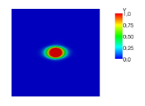
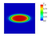
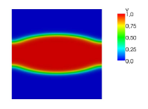
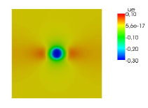
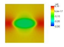
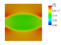
Figure 3. Reference solution in the two-dimensional case. Above: spreading of the transmembrane potential $v$ excitation wave. From left to right, the three pictures correspond to times $t$=0.2, 0.6 and 1.2 after the stimulation initiation, stimulation duration being 0.1. Below: associated extracellular potential $u_{e}$.

Excitation is initiated by applying a centred stimulation during a short period of time, precisely: $I_{\mathrm{app}}(x,t)=0.9$ for $1<t<1.1$ and $|x-x_{0}|<0.1$ ($x_{0}$ denoting the centre of ${\Omega}$) and $I_{\mathrm{app}}(x,t)=0$ otherwise. The initial condition for $v$ is uniformly set to 0. A homogeneous Neumann boundary condition is considered on $\partial{\Omega}$, uniqueness is ensured by adding the normalisation condition (4) on $u_{e}$. The domain ${\Omega}$ is assumed to be composed of a bundle of parallel horizontal muscular fibres, resulting in the following choice for the anisotropy tensors $\mathbf{M}_{i}(x)$ and $\mathbf{M}_{e}(x)$:

(58) $$\mathbf{M}_{i}(x)=\text{Diag}(\lambda_{i}^{l},\lambda_{i}^{t},\lambda_{i}^{t})~{},\quad\mathbf{M}_{e}(x)=\text{Diag}(\lambda_{e}^{l},\lambda_{e}^{t},\lambda_{e}^{t})~{},$$

the values for the longitudinal ($l$) and transverse ($t$) conductivities for the intra and extra-cellular medias have been taken from [42]: the resulting anisotropy ratios for the intra and extra-cellular medias respectively are 9.0 and 2.0 between the longitudinal and transverse directions.

The numerical solution for the transmembrane potential $v$ takes the form of an excitation wave propagating across the domain from the stimulation site towards the boundary and from the rest potential $v=0$ to the activation potential $v=1$. A sharp but smooth wavefront for $v$ displays an elliptic shape away from the boundary, which is induced by the media anisotropy. A reference solution is generated on a mesh using a 1 147 933 (resp. 479 873) nodes in dimension 3 (resp. 2).

7.2. Implementation

Let us fix a mesh ${\boldsymbol{\mathfrak{T}}}$. For simplicity, discrete functions $w,v\in{\mathbb{R}}^{\scriptscriptstyle\boldsymbol{\mathfrak{T}}}$ will also be considered as one-column real matrices in this subsection, $w^{T}$, $v^{T}$ denoting their transpose one-row real matrices. Let us first introduce the mass matrix (diagonal here) $\Lambda\in\text{Mat}({\mathbb{R}}^{\scriptscriptstyle\boldsymbol{\mathfrak{T}}})$:

$$\forall w,v\in{\mathbb{R}}^{\scriptscriptstyle\boldsymbol{\mathfrak{T}}}:\quad{\biggl{[}\biggl{[}}w,v{\biggr{]}\biggr{]}}_{{\Omega}}=w^{T}\Lambda v.$$

Relative to (58), uniform discrete tensors $\mathbf{M}_{i,e}^{\scriptscriptstyle\boldsymbol{\mathfrak{T}}}$ are considered here, with value

$$\mathbf{M}_{i}^{\scriptscriptstyle\boldsymbol{\mathfrak{T}}}=\text{Diag}(\lambda_{i}^{l},\lambda_{i}^{t},\lambda_{i}^{t})~{},\quad\mathbf{M}_{e}^{\scriptscriptstyle\boldsymbol{\mathfrak{T}}}=\text{Diag}(\lambda_{e}^{l},\lambda_{e}^{t},\lambda_{e}^{t})~{},$$

on each diamond ${\scriptstyle D}$. The discrete gradient being defined relative to the homogeneous Neumann boundary condition, and simply denoted by ${\,\nabla}^{\scriptscriptstyle\boldsymbol{\mathfrak{T}}}$, the two stiffness matrices $\Sigma_{i}$ and $\Sigma_{e}$ are introduced as:

$$\forall w,v\in{\mathbb{R}}^{\scriptscriptstyle\boldsymbol{\mathfrak{T}}}:\quad{\biggl{\{}\!\!\!\biggl{\{}}\mathbf{M}_{i}^{\scriptscriptstyle\boldsymbol{\mathfrak{T}}}{\,\nabla}^{\scriptscriptstyle\boldsymbol{\mathfrak{T}}}v,{\,\nabla}^{\scriptscriptstyle\boldsymbol{\mathfrak{T}}}w{\biggr{\}}\!\!\!\biggr{\}}}_{{\Omega}}=v^{T}\Sigma_{i}w,\quad{\biggl{\{}\!\!\!\biggl{\{}}\mathbf{M}_{e}^{\scriptscriptstyle\boldsymbol{\mathfrak{T}}}{\,\nabla}^{\scriptscriptstyle\boldsymbol{\mathfrak{T}}}v,{\,\nabla}^{\scriptscriptstyle\boldsymbol{\mathfrak{T}}}w{\biggr{\}}\!\!\!\biggr{\}}}_{{\Omega}}=v^{T}\Sigma_{e}w.$$

These stiffness matrices are positive, symmetric matrices, although not definite since a Neumann homogeneous boundary condition is considered.

The following semi-implicit Euler scheme is considered: given $v^{n},I_{\mathrm{app}}^{n}\in{\mathbb{R}}^{\scriptscriptstyle\boldsymbol{\mathfrak{T}}}$, determine $v^{n+1},u_{e}^{n+1}\in{\mathbb{R}}^{\scriptscriptstyle\boldsymbol{\mathfrak{T}}}$ such that,

(59) $$\left\{\begin{array}[]{l}\displaystyle{\rm div\,}^{\scriptscriptstyle\boldsymbol{\mathfrak{T}}}[(\mathbf{M}_{e}^{\scriptscriptstyle\boldsymbol{\mathfrak{T}}}+\mathbf{M}_{i}^{\scriptscriptstyle\boldsymbol{\mathfrak{T}}}){\,\nabla}^{\scriptscriptstyle\boldsymbol{\mathfrak{T}}}u_{e}^{n+1}]+{\rm div\,}^{\scriptscriptstyle\boldsymbol{\mathfrak{T}}}\left[\mathbf{M}_{i}^{\scriptscriptstyle\boldsymbol{\mathfrak{T}}}{\,\nabla}^{\scriptscriptstyle\boldsymbol{\mathfrak{T}}}v^{n+1}\right]=0,\\[5.0pt] \displaystyle\varepsilon\frac{v^{n+1}-v^{n}}{{{\scriptstyle\Delta}t}}+\varepsilon^{2}{\rm div\,}^{\scriptscriptstyle\boldsymbol{\mathfrak{T}}}[\mathbf{M}_{e}^{\scriptscriptstyle\boldsymbol{\mathfrak{T}}}{\,\nabla}^{\scriptscriptstyle\boldsymbol{\mathfrak{T}}}u_{e}^{n+1}]+h[v^{n}]=I_{\mathrm{app}}^{n}.\end{array}\right.$$

Writing separately the scalar product ${\biggl{[}\biggl{[}}\cdot,\cdot{\biggr{]}\biggr{]}}_{{\Omega}}$ of each line in (59) with all test functions $w\in{\mathbb{R}}^{\scriptscriptstyle\boldsymbol{\mathfrak{T}}}$ and using the discrete duality (11) leads to the following equivalent formulation written in matrix form:

(60) $$M\left|\begin{array}[]{l}\displaystyle u_{e}^{n+1}\\[15.0pt] \displaystyle v^{n+1}\end{array}\right.=\left|\begin{array}[]{l}\displaystyle 0\\[15.0pt] \displaystyle\Lambda[v^{n}+{{\scriptstyle\Delta}t}(I_{\mathrm{app}}^{n}-h[v^{n}])/\varepsilon]\end{array}\right.~{}~{},\quad M:=\left[\begin{array}[]{cc}\displaystyle\Sigma_{i}+\Sigma_{e}&\Sigma_{i}\\[5.0pt] \displaystyle-\varepsilon{{\scriptstyle\Delta}t}\Sigma_{e}&\Lambda\end{array}\right].$$

To ensure uniqueness on $u_{e}$, the normalisation condition (4) is discretised as:

(61) $${\biggl{[}\biggl{[}}u_{e}^{n+1},U^{\scriptscriptstyle\boldsymbol{\mathfrak{M}}^{o}}{\biggr{]}\biggr{]}}_{{\Omega}}=0={\biggl{[}\biggl{[}}u_{e}^{n+1},U^{\scriptscriptstyle\boldsymbol{\mathfrak{M}}^{*}}{\biggr{]}\biggr{]}}_{{\Omega}},$$

where $U^{\scriptscriptstyle\boldsymbol{\mathfrak{M}}^{o}}$ (resp. $U^{\scriptscriptstyle\boldsymbol{\mathfrak{M}}^{*}}$) is the discrete function equal to 1 relatively to each primal (resp. dual) control volumes and to 0 elsewhere.

The implementation of (60) therefore reads as a three-step algorithm:

at each time step,

1. compute $y_{2}:=\Lambda[v^{n}+{{\scriptstyle\Delta}t}(I_{\mathrm{app}}^{n}-h[v^{n}])/\varepsilon]$. The matrix $\Lambda$ being diagonal, computations for this step are cheap;

2. determine a solution $x=(u_{e}^{n+1},v^{n+1})^{T}$ to the global system $Mx=y$ for $y=(0,y_{2})^{T}$;

3. normalise $u_{e}^{n+1}$ using condition (61). For the same reason as for step one, this step is a cheap one.

Because of the large size of the considered problem (1.1 million of nodes in 3D for the most refined mesh, i.e. 2.2 million of lines for the matrix $M$) and because of the relatively non-compact sparsity pattern for $M$ in 3D, step 2 is not an easy task. Therefore, a careful attention has to be paid to the preconditioning of $M$: the strategy adopted here is detailed in [50].

7.3. Numerical tests and results

The convergence of the DDFV scheme is numerically analysed comparing the reference solution described in Subsection 7.1 with numerical solutions obtained on coarser meshes. In 3D, four tetrahedral meshes have been considered: from 2 559 to 1 147 933 nodes, between two meshes the mesh size is divided by 2, two successive meshes are not obtained via refinement. In 2D, six meshes are used: from 489 to 479 873 nodes. The time step ${{\scriptstyle\Delta}t}$ is also divided by two each time the space resolution is divided by 2; the starting time step (on the coarsest mesh) is 0.02.

To compare numerical solutions defined on different meshes, a projection is needed: this is done as follows. Let ${\boldsymbol{\mathfrak{T}}}^{r}$ and ${\boldsymbol{\mathfrak{T}}}^{c}$ be the reference mesh and a coarser mesh respectively, and let ${\mathbb{R}}^{{\scriptscriptstyle\boldsymbol{\mathfrak{T}}}_{r}}$, ${\mathbb{R}}^{{\scriptscriptstyle\boldsymbol{\mathfrak{T}}}_{c}}$ respectively denote the associated spaces of discrete functions. Consider the simplicial mesh $\mathcal{S}^{r}$ (respectively $\mathcal{S}^{c}$) whose cells are obtained by cutting all diamonds of ${\boldsymbol{\mathfrak{T}}}^{r}$ (resp. ${\boldsymbol{\mathfrak{T}}}^{c}$) in two along the interface. A discrete function $u^{r}\in{\mathbb{R}}^{{\scriptscriptstyle\boldsymbol{\mathfrak{T}}}_{r}}$ (resp. $u^{c}\in{\mathbb{R}}^{{\scriptscriptstyle\boldsymbol{\mathfrak{T}}}_{c}}$) consists in one scalar associated to each vertex and each cell centre of the mesh ${\boldsymbol{\mathfrak{T}}}^{r}$ (resp. ${\boldsymbol{\mathfrak{T}}}^{c}$), thus to each vertex of $\mathcal{S}^{r}$ (resp. $\mathcal{S}^{c}$). It is therefore natural to associate to $u^{c}$ (resp. $u^{r}$) the continuous function $\tilde{u}^{r}$ (resp. $\tilde{u}^{c}$) piecewise affine on the cells of $\mathcal{S}^{r}$ (resp. $\mathcal{S}^{c}$) and whose values at the vertices of $\mathcal{S}^{r}$ (resp. $\mathcal{S}^{c}$) are given by the discrete function $u^{r}$ (resp. $u^{c}$). A projection $u^{c\to r}\in{\mathbb{R}}^{{\scriptscriptstyle\boldsymbol{\mathfrak{T}}}_{r}}$ of a (coarse) discrete function $u^{c}\in{\mathbb{R}}^{{\scriptscriptstyle\boldsymbol{\mathfrak{T}}}_{c}}$ is then simply defined by computing the values of the function $\tilde{u}^{c}$ on the vertices of $\mathcal{S}^{r}$. The relative error between $u^{r}\in{\mathbb{R}}^{{\scriptscriptstyle\boldsymbol{\mathfrak{T}}}_{r}}$ and $u^{c}\in{\mathbb{R}}^{{\scriptscriptstyle\boldsymbol{\mathfrak{T}}}_{c}}$ in $L^{2}({\Omega})$ norm is defined as

(62) $$e_{{\Omega},2}(u^{r},u^{c})^{2}:=\dfrac{\int_{\Omega}|\tilde{u}^{r}-\tilde{u}^{c\to r}|^{2}dx}{\int_{\Omega}|\tilde{u}^{r}|^{2}dx}.$$

Numerically, these integrals are evaluated using an order two Gauss quadrature on the cells of $\mathcal{S}^{r}$, leading to an exact evaluation up to rounding errors.

The three following tests have been performed.

7.3.1. Test 1; activation time convergence

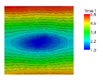
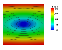
Figure 4. Activation time in dimension 2 for three different meshes, the isolines (in black) are separated by 1/3 unit of time. The stimulation is initiated at time $t=1$. From the left (coarsest mesh) to the right (reference solution) the three different activation time mappings have been computed on meshes with 439, 7569 and 479 873 nodes respectively.

The activation time mapping $\phi:~{}{\Omega}\mapsto\mathbb{R}$ is defined at each point $x$ as the time $\phi(x)=t$ such that the transmembrane potential $v(x,t)=s$ for the threshold value $s:=0.9$. The value $\phi(x)$ tells us at what time the excitation wave reaches the point $x$, the activation time mapping thus is of crucial importance in terms of physiological interpretation of the model. Activation time in 2D computed on various meshes are depicted on Figure 4. The discrepancy between the activation mappings $\phi^{r}$ and $\phi^{c}$ computed at the reference and coarse levels respectively is evaluated using the relative error in the $L^{2}({\Omega})$ norm defined in (62). Numerical results for activation time convergence are given in Table 1.

# nodes errors $e_{{\Omega},2}$ 489 1.611 1913 9.130 $10^{-2}$ 7 569 1.776 $10^{-2}$ 30 113 4.850 $10^{-3}$ 120 129 1.139 $10^{-3}$ 479 873 reference		# nodes errors $e_{{\Omega},2}$ 2 559 1.110 19 500 8.195 $10^{-2}$ 148 242 1.281 $10^{-2}$ 1 147 933 reference
2D case		3D case

Table 1. Activation time mappings convergence. The errors are relative errors in $L^{2}({\Omega})$ norm as defined in (62)

Convergence is numerically observed here both in 2D and in 3D. Moreover, the figures obtained in the two dimensional case indicate an order two convergence relatively to the mesh size. Such a conclusion, although plausible, is not possible in the three dimensional case: to be observed it would require a much finer reference mesh which is not affordable in terms of computational effort.

7.3.2. Test 2; space convergence

Let us denote by $v^{r}$ and $u_{e}^{r}$, (resp. $v^{c}$ and $u_{e}^{c}$) the transmembrane potential and extracellular potential computed on the reference mesh (resp. a coarse mesh). The discrepancy between $v^{c}$, $v^{r}$ and $u_{e}^{r}$, $u_{e}^{c}$ at a chosen time $t$ has been computed using the relative error in the $L^{2}({\Omega})$ norm (62). Three fixed times $t$ have been considered: $t=$ 1.2, 1.6 and 2.2, corresponding to the reference solution depicted in Figure 3.

# nodes $t=1.2$ $t=1.6$ $t=2.2$ $t=1.2$ $t=1.6$ $t=2.2$ 489 0.51 0.37 0.45 0.45 0.34 0.59 1913 0.24 8.87 $10^{-2}$ 0.14 0.22 8.27 $10^{-2}$ 0.17 7569 0.13 6.01 $10^{-2}$ 1.42 $10^{-2}$ 0.12 5.38 $10^{-2}$ 1.99 $10^{-2}$ 30113 6.24 $10^{-2}$ 3.29 $10^{-2}$ 1.28 $10^{-2}$ 5.62 $10^{-2}$ 2.89 $10^{-2}$ 1.71 $10^{-2}$ 120129 1.25 $10^{-2}$ 5.26 $10^{-3}$ 1.74 $10^{-3}$ 1.13 $10^{-2}$ 5.31 $10^{-3}$ 2.86 $10^{-3}$

2D case

# nodes $t=1.2$ $t=1.6$ $t=2.2$ $t=1.2$ $t=1.6$ $t=2.2$ 2559 0.43 0.57 0.65 0.42 0.63 0.91 19 500 0.22 0.14 0.20 0.19 0.17 0.28 148 242 0.10 6.21 $10^{-2}$ 2.88 $10^{-2}$ 9.45 $10^{-2}$ 6.40 $10^{-2}$ 4.33 $10^{-2}$

3D case

Table 2. Convergence of the transmembrane potential $v$ and of the extracellular potential $u_{e}$ at three fixed times: $t=$ 1.2, 1.6 and 2.2. The reference solution for these chosen times are depicted in Figure 3. Above (resp. below) are reported the errors in the two (resp. three) dimensional case. On each table line the three first figures after the number of nodes correspond to the errors on $v$, whereas the three last ones correspond to $u_{e}$. Errors are relative errors in $L^{2}({\Omega})$ norm as defined in (63).

Because of the particular wavefront-like shape of the solution, this error can be geometrically reinterpreted as follows. Consider at time $t$ the sub-region of ${\Omega}$ that is activated according to the reference solution $u_{e}^{r}$ but not activated according to the coarse solution $u_{e}^{c}$. The numerator in (63) simply measures the square root of the area of this sub-region. Using the elliptic shape of activated regions, one gets that $e_{{\Omega},2}(u^{r},u^{c})$ measures the square root of the relative error on the wavefront propagation velocity (more precisely the square root of the sum of the axial and transverse wavefront propagation velocities relative errors). This error, as in test case 1, is of prime physiological importance. Numerical results for this test are displayed in Table 2. Although convergence is well illustrated, no particular asymptotic behaviour can be inferred from these results.

7.3.3. Test 3; space and time convergence

A numerical space and time convergence indicator $e_{Q,2}$ is introduced here, aiming to reproduce an $L^{2}(Q)$ relative error between a coarse and the reference solution ($Q=(0,T)\times{\Omega}$). Convergence is measured using this indicator, and this third test therefore is intended to numerically illustrate the convergence result of Theorem 4.5.

# nodes errors $e_{Q,2}$ 489 0.481 1913 0.237 7569 6.469 $10^{-2}$ 30113 1.746 $10^{-2}$ 120129 4.167 $10^{-3}$ 479 873 reference		# nodes errors $e_{Q,2}$ 2559 0.673 19 500 0.219 148 242 4.920 $10^{-2}$ 1 147 933 reference
2D case		3D case

Table 3. Space and time convergence for the transmembrane potential $v$. Errors are relative errors in the $L^{2}(Q)$ norm as defined in (63)

The transmembrane potentials $v^{r}$ and $v^{c}$ have been recorded at the same times, namely $t_{n}=n\delta t$, for $\delta t=1/100$ unit of time, $n=0,\dots,T/\delta t$ and $T=3$. The corresponding numerical solutions are denoted $v^{r}_{n}$ and $v^{c}_{n}$. A relative error in the $L^{2}(Q)$ norm between $v^{r}$ and $v^{c}$ is introduced as follows:

(63) $$e_{Q,2}(v^{r},v^{c})^{2}:=\dfrac{\sum_{n=0}^{N}\int_{\Omega}|\tilde{v_{n}}^{r}-\tilde{v_{n}}^{c\to r}|^{2}dx\delta t}{\sum_{n=0}^{N}\int_{\Omega}|\tilde{v_{n}}^{r}|^{2}dx\delta t}~{},\quad N=T/\delta t.$$

Numerical results are given in Table 3: convergence both in 2D and in 3D is observed. The two dimensional case results indicate an order two convergence relatively to the mesh size. As in the first test case, such a conclusion is not possible in the three dimensional case: a much finer reference mesh (not affordable) would be needed.

References

- [1] H.W. Alt and S. Luckhaus. Quasilinear elliptic-parabolic differential equations. Math. Z. 183:311-341, 1983.
- [2] B. Andreianov, M. Bendahmane and F. Hubert. On finite volume discretisation of gradient and divergence operators in 3D. Preprint HAL.
- [3] B. Andreianov, M. Bendahmane and K.H. Karlsen. A gradient reconstruction formula for finite volume schemes and discrete duality. In R. Eymard and J. M. Herard, eds., Proceedings of Finite Volumes for Complex Applications V, Hermès, 2008.
- [4] B. Andreianov, M. Bendahmane and K.H. Karlsen. Discrete duality finite volume schemes for doubly nonlinear degenerate hyperbolic-parabolic equations. J. Hyperbolic Differ. Equ., 7(1):1-67, 2010.
- [5] B. Andreianov, M. Bendahmane and R. Ruiz Baier. Analysis of a finite volume method for a cross-diffusion model in population dynamics. M3AS Math. Models Meth. Appl. Sci., to appear.
- [6] B. Andreianov, F. Boyer, and F. Hubert. Discrete duality finite volume schemes for Leray-Lions type elliptic problems on general 2D meshes. Num. Meth. PDE, 23(1):145–195, 2007.
- [7] B. Andreianov, M. Gutnic, and P. Wittbold. Convergence of finite volume approximations for a nonlinear elliptic-parabolic problem: a ”continuous” approach. SIAM J. Numer. Anal. 42(1):228–251, 2004.
- [8] M. Bendahmane and K.H. Karlsen. Analysis of a class of degenerate reaction-diffusion systems and the bidomain model of cardiac tissue. Netw. Heterog. Media 1:185–218, 2006.
- [9] M. Bendahmane and K.H. Karlsen. Convergence of a finite volume scheme for the bidomain model of cardiac tissue. Appl. Numer. Math., 59(9):2266–2284, 2009.
- [10] M. Bendahmane, R. Bürger, and R. Ruiz Baier. A finite volume scheme for cardiac propagation in media with isotropic conductivities. Math. Comp. Simul., 80:1821–1840, 2010.
- [11] S. Börm, L. Grasedyck, and W. Hackbusch. An introduction to hierarchical matrices Mathematica Bohemica 127(2):229-241, 2002.
- [12] S. Börm, L. Grasedyck and W. Hackbusch Introduction to hierarchical matrices with applications Eng. Anal. Bound. 27:405-422, 2003.
- [13] Y. Bourgault, Y. Coudière, and C. Pierre. Existence and uniqueness of the solution for the bidomain model used in cardiac electro-physiology. Nonlin. Anal. Real World Appl. 10:458–482, 2009.
- [14] F. Boyer and P. Fabrie. Eléments d’analyse pour l’étude de quelques modèles d’écoulements de fluides visqueux incompressibles. Mathématiques&Applications Vol.52, Springer-Verlag, Berlin, 2006.
- [15] F. Boyer and F. Hubert. Finite volume method for 2D linear and nonlinear elliptic problems with discontinuities. SIAM J. Num. Anal. 46(6):3032–3070, 2008.
- [16] P. Colli Franzone, L. Guerri, and S. Rovida. Wavefront propagation in an activation model of the anisotropic cardiac tissue: asymptotic analysis and numerical simulations. J. Math. Biol., 28(2):121–176, 1990.
- [17] P. Colli Franzone, L. Guerri, and S. Tentoni. Mathematical modeling of the excitation process in myocardial tissue: Influence of fiber rotation on wavefront propagation and potential field. Math. Biosci. 101(2):155–235, 1990.
- [18] P. Colli Franzone, L.F. Pavarino, and B. Taccardi. Simulating patterns of excitation, repolarization and action potential duration with cardiac Bidomain and Monodomain models. Math. Biosci., 197(1):35–66, 2005.
- [19] P. Colli Franzone and G. Savaré. Degenerate evolution systems modeling the cardiac electric field at micro- and macroscopic level. In Evolution equations, semigroups and functional analysis (Milano, 2000), volume 50 of Progr. Nonlinear Differential Equations Appl., pp. 49–78. Birkhäuser, Basel, 2002.
- [20] Y. Coudière, Th. Gallouët and R. Herbin. Discrete Sobolev inequalities and error estimates for finite volume solutions of convection diffusion equations. M2AN Math. Model. Numer. Anal. 35(4):767?-778, 2001.
- [21] Y. Coudière and F. Hubert. A 3D Discrete Duality Finite Volume method for nonlinear elliptic equations. Preprint HAL.
- [22] Y. Coudière and C. Pierre. Stability and convergence of a finite volume method for two systems of reaction-diffusion in electro-cardiology. Nonlin. Anal. Real World Appl. 7:916–935, 2006.
- [23] Y. Coudière, C. Pierre and R. Turpault. A 2D/3D Finite Volume Method used to solve the bidomain equations of electro-cardiology. Proceedings of Algorithmy 2009, 18th Conference on Scientific Computing(2009), 1-10.
- [24] Y. Coudière, C. Pierre, R. Turpault, and O. Rousseau. A 2D/3D Discrete Duality Finite Volume Scheme. Application to ECG simulation. International Jourmal on Finite Volumes, 6(1), 2008.
- [25] K. Domelevo, S. Delcourte and P. Omnes. Discrete-duality finite volume method for second order elliptic equations, in: F. Benkhaldoun, D. Ouazar, S. Raghay (Eds.), Finite Volumes for Complex Applications, Hermes Science Publishing, 2005, pp. 447–458.
- [26] K. Domelevo and P. Omnès. A finite volume method for the Laplace equation on almost arbitrary two-dimensional grids. M2AN Math. Model. Numer. Anal. 39(6):1203–1249, 2005.
- [27] L. C. Evans, Partial differential equations, volume 19 of Graduate Studies in Mathematics. American Mathematical Society, Providence, RI, 1998.
- [28] R. Eymard, T. Gallouët, and R. Herbin. Finite Volume Methods. Handbook of Numerical Analysis, Vol. VII, P. Ciarlet, J.-L. Lions, eds., North-Holland, 2000.
- [29] R. Eymard, T. Gallouët, and R. Herbin. Discretisation of heterogeneous and anisotropic diffusion problems on general non-conforming meshes. SUSHI: a scheme using stabilisation and hybrid interfaces, IMA J. Numer. Anal.( doi:10.1093/imanum/drn084 ), 2009.
- [30] A. Glitzky and J.A. Griepentrog. Discrete Sobolev-Poincaré inequalities for Voronoï finite volume approximations. Preprint 2009, WIAS Berlin.
- [31] D. Harrild and C.S. Henriquez. A finite volume model of cardiac propagation. Ann. Biomed. Engrg. 25:315–334, 1997.
- [32] R. Herbin and F. Hubert. Benchmark on discretisation schemes for anisotropic diffusion problems on general grids, in R. Eymard and J. M. Herard, eds., Proceedings of Finite Volumes for Complex Applications V, Hermès, 2008
- [33] C. S. Henriquez. Simulating the electrical behavior of cardiac tissue using the biodomain models. Crit. Rev. Biomed. Engr., 21:1–77, 1993.
- [34] F. Hermeline. Une méthode de volumes finis pour les équations elliptiques du second ordre. C. R. Math. Acad. Sci. Paris 326(12):1433–1436, 1998.
- [35] F. Hermeline. A finite volume method for the approximation of diffusion operators on distorted meshes. J. Comput. Phys. 160(2):481–499, 2000.
- [36] F. Hermeline. A finite volume method for solving Maxwell equations in inhomogeneous media on arbitrary meshes. C. R. Math. Acad. Sci. Paris 339(12):893–898, 2004.
- [37] F. Hermeline. Approximation of 2D and 3D diffusion operators with discontinuous full-tensor coefficients on arbitrary meshes. Comput. Meth. Appl. Mech. Engrg. 196:2497–2526, 2007.
- [38] F. Hermeline. A finite volume method for approximating 3D diffusion operators on general meshes. Comput. Meth. Appl. Mech. Engrg., 2009.
- [39] A.L. Hodgkin and A.F. Huxley. A quantitative description of membrane current and its application to conduction and excitation in nerve. J. Physiol., 117(4):500–544, 1952.
- [40] J. Keener and J. Sneyd. Mathematical physiology. Volume 8 of Interdisciplinary Applied Mathematics. Springer-Verlag, New York, 1998.
- [41] S.N. Kruzhkov. Results on the nature of the continuity of solutions of parabolic equations and some of their applications. Mat. Zametki 6(1):97–108, 1969; english tr. in Math.Notes 6(1):517-523, 1969.
- [42] P. Le Guyader, F. Trelles, and P. Savard. Extracellular measurement of anisotropic bidomain myocardial conductivities. I. theoretical analysis. Annals Biomed. Eng., 29(10):862–877, 2001.
- [43] G.T. Lines, P. Grottum, A.J. Pullan, J. Sundes, and A. Tveito. Mathematical models and numerical methods for the forward problem in cardiac electrophysiology. Comput. Visual. Sci, 5:215–239, 2002.
- [44] G. Lines, M.L. Buist, P. Grøttum, A.J. Pullan, J. Sundnes, and A. Tveito, Mathematical models and numerical methods for the forward problem in cardiac electrophysiology. Computing and Visualization in Science, 5(4):215–239, 2003.
- [45] J.-L. Lions and E. Magenes. Problèmes aux limites non homogènes et applications. Volume 1. (French) Dunod, Paris, 1968.
- [46] C.-H. Luo and Y. Rudy. A model of the ventricular cardiac action potential. Depolarization, repolarization, and their interaction. Circ Res., 68(6):1501–1526, 1991.
- [47] D. Noble. A modification of the Hodgkin-Huxley equation applicable to Purkinje fibre action and pacemaker potentials. J. Physiol., 160:317–352, 1962.
- [48] F. Otto. -contraction and uniqueness for quasilinear elliptic-parabolic equations. J. Diff. Eq. 131(1):20–38, 1996.
- [49] C. Pierre. Modélisation et simulation de l’activité électrique du coeur dans le thorax, analyse numérique et méthodes de volumes finis. Ph.D. Thesis, Université de Nantes, 2005.
- [50] C. Pierre. Preconditioning the coupled heart and torso bidomain model with an almost linear complexity. HAL Preprint, 2010.
- [51] S. Sanfelici. Convergence of the Galerkin approximation of a degenerate evolution problem in electro-cardiology. Numer. Methods PDE, 18(2):218–240, 2002.
- [52] J. Sundnes, G.T. Lines, X. Cai, B.F. Nielsen, K.-A. Mardal, and A. Tveito. Computing the electrical activity in the human heart. Springer-Verlag, 2005.
- [53] J. Sundnes, G.T. Lines, and A. Tveito. An operator splitting method for solving the bidomain equations coupled to a volume conductor model for the torso. Math. Biosciences, 194(2):233–248 (2005).
- [54] L. Tung. A bidomain model for describing ischemic myocardial D-D properties. Ph.D. thesis, M.I.T.., 1978.
- [55] M. Veneroni. Reaction-diffusion systems for the microscopic cellular model of the cardiac electric field. Math. Methods Appl. Sci., 29(14):1631–1661, 2006.