Gaussian flexibility with Fourier accuracy: the periodic von Neumann basis set

Abstract

We propose a new method for solving quantum mechanical problems, which combines the flexibility of Gaussian basis set methods with the numerical accuracy of the Fourier method. The method is based on the incorporation of periodic boundary conditions into the von Neumann basis of phase space Gaussians [F. Dimler et al., New J. Phys. 11, 105052 (2009)]. In this paper we focus on the Time-independent Schrödinger Equation and show results for the harmonic, Morse and Coulomb potentials that demonstrate that the periodic von Neumann method or pvN is significantly more accurate than the usual vN method. Formally, we are able to show an exact equivalence between the pvN and the Fourier Grid Hamiltonian (FGH) methods. Moreover, due to the locality of the pvN functions we are able to remove Gaussian basis functions without loss of accuracy, and obtain significantly better efficiency than that of the FGH. We show that in the classical limit the method has the remarkable efficiency of 1 basis function per 1 eigenstate.

The formal framework for quantum mechanics is an infinite dimensional Hilbert space. In any numerical calculation, however, a wave function is represented in a finite dimensional basis set and therefore the choice of basis set determines the accuracy. The optimal basis set should combine accuracy and flexibility, allowing a small number of basis functions to represent the wave functions even in the presence of complex boundary conditions and geometry. Unfortunately, these two criteria —accuracy and efficiency— are usually in conflict, and globally accurate methods fourier_method ; fgh ; wei lack the flexibility of local methods dgb ; garashchuk . For example, in the pseudospectral Fourier grid method the wave function is represented by its values on a finite number of evenly spaced grid points. Due to the Nyquist sampling theorem, this allows for an exact representation of the wave provided the wavefunction is band limited with finite supportwhittaker ; nyquist ; shannon . However, the non-local form of the basis functions in momentum space leads to limited efficiency. On the other hand, in the von Neumann basis set brixner ; von_neumann each basis function is localized on a unit cell of size $h$ in phase space. However, despite the formal completeness of the vN basis setperelomov , attempts to utilize this basis in quantum numerical calculations have been plagued with numerical errorsdavis_and_heller ; poirier .

The purpose of this paper is to establish a precise mathematical formalism for the von Neumann basis on a truncated phase space. This allows us to demonstrate an exact equivalence with the Fourier method while retaining the flexibility of a Gaussian basis. It puts on a rigorous basis the seminal work of Dimler et al.dimler who used a vN basis with periodic boundary conditions, although in our formalism the periodicity of the vN basis appears only implicitly.

The von Neumann basis set von_neumann is a subset of the “coherent states” of the form:

$$g_{nl}(x)=\left(\frac{2\alpha}{\pi}\right)^{\frac{1}{4}}\exp\left(-\alpha(x-na)^{2}-il\dfrac{2\pi\hbar}{a}(x-na)\right)$$ (1)

where $n$ and $l$ are integers. Each basis function is a Gaussian centered at $(na,\frac{2\pi l}{a})$ in phase space. The parameter $\alpha=\frac{\sigma_{p}}{2\sigma_{x}}$ controls the FWHM of each Gaussian in $x$ and $p$ space. Taking $\Delta x=a,\Delta p=h/a$ as the spacing between neighboring Gaussians in $x$ and $p$ space respectively, we note that $\Delta x\Delta p=h$ so we have exactly one basis function per unit cell in phase space. As shown inperelomov this implies completeness in the Hilbert space.

The “complete” vN basis, where $n$ and $l$ run over all integers, spans the infinite Hilbert space. In any numerical calculation, however, $n$ and $l$ take on a finite number of values, producing $N$ Gaussian basis functions $\{g_{i}(x)\}$, $i=1...N$. Since the size of one vN unit cell is $h$, the area of the truncated vN lattice is given by $S^{\rm vN}=Nh$.

In the pseudospectral Fourier method, a function $\psi(x)$ that is periodic in $L$ and band limited in $K=\frac{P}{\hbar}$ can be written in the following form: $\psi(x)=\sum_{n=1}^{N}\psi(x_{n})\theta_{n}(x)$, where $x_{n}=\delta_{x}(n-1)$, and $\delta_{x}=\frac{\pi\hslash}{P}=\frac{L}{N}$. The basis functions $\{\theta_{n}(x)\}$ are given by tannor_book :

$$\theta_{n}(x)=\sum_{j=\frac{-N}{2}+1}^{\frac{N}{2}}\frac{1}{\sqrt{LN}}\exp\left(\frac{i2\pi j}{L}(x-x_{n})\right),$$ (2)

which can be shown to be sinc functions that are periodic on the domain $[0,L]$. The set $\{\theta_{i}(x)\}$ $i=1,..,N$ spans a rectangular shape in phase space with area of $S^{\rm FGH}=2LP=2L\frac{\pi\hbar}{\delta_{x}}=Nh$. Thus $N$ unit cells in the vN lattice and $N$ grid points in the Fourier method cover the same rectangle with an area in phase space of:

$$S^{\rm vN}=S^{\rm FGH}=Nh$$ (3)

(Fig. 1). This suggests that $N$ vN basis functions confined to this area will be equivalent to the Fourier basis set. Unfortunately, the attempt to use $N$ Gaussians as a basis set for the area in eq.(3) (Fig. 1) is unsuccessful, a consequence of the Gaussians on the edges protruding from the truncated space. However, by combining the Gaussian and the Fourier basis functions we can generate a “Gaussian-like” basis set that is confined to the truncated space. We use the basis sets $\{g_{i}(x)\}$ and $\{\theta_{i}(x)\}$ to construct a new basis set, $\{\tilde{g}_{i}(x)\}$:

$$\tilde{g}_{m}(x)=\sum_{n=1}^{N}\theta_{n}(x)g_{m}(x_{n})$$ (4)

for $m=1,...,N$. The new basis set is in some sense, the Gaussian functions with periodic boundary conditions. We can write eq.(4) in matrix notation as: $\tilde{G}=\Theta G$ where $G_{ij}=g_{j}(x_{i})$ By taking the width parameter $\alpha=\frac{\Delta p}{2\Delta x}$ we can guarantee that the pvN functions have no linear dependence and that the matrix $G$ is invertible, that is $\tilde{G}G^{-1}=\Theta$. The invertibility of $G$ implies that both bases span the same space.

The representation of $|\psi\rangle$ in the pvN basis set is given by:

$$|\psi\rangle=\sum_{m=1}^{N}|\tilde{g}_{m}\rangle a_{m}.$$ (5)

To find the coefficients $a_{m}$ we first define the overlap matrix, $S$:

$$S_{ij} = \langle\tilde{g}_{i}|\tilde{g}_{j}\rangle=\int_{0}^{L}\tilde{g}_{i}^{*}(x)\tilde{g}_{j}(x)dx$$ (6)

$$= \sum_{n=1}^{N}\sum_{m=1}^{N}g_{i}^{*}(x_{n})g_{j}(x_{m})\int_{0}^{L}\theta_{n}^{*}(x)\theta_{m}(x)dx$$

$$= \sum_{n=1}^{N}g_{i}^{*}(x_{n})g_{j}(x_{n})$$

or

$$S=G^{{\dagger}}G.$$ (7)

Using the completeness relationship for non-orthogonal bases, $|\psi\rangle$ can be expressed as

$$|\psi\rangle=\sum_{n=1}^{N}\sum_{m=1}^{N}|\tilde{g}_{m}\rangle(S^{-1})_{mn}\langle\tilde{g}_{n}|\psi\rangle.$$ (8)

Comparing with eq.(5) we find that $a_{m}=\sum_{n=1}^{N}(S^{-1})_{mn}\langle\tilde{g}_{n}|\psi\rangle$ and $\langle\tilde{g}_{i}|\psi\rangle=\sum_{n=1}^{N}g_{i}^{*}(x_{n})\psi(x_{n})$.

Figure 1: $N=9$ coordinate grid points and $N=9$ vN unit cells span the same area in phase space,$S=Nh$. The vN basis functions are Gaussians located at the center of each unit cell.

Although the periodic von Neumann (pvN) and the Fourier methods span the same rectangle in phase space, the localized nature of the basis functions in the pvN method can lead to significant advantages. In particular, if $|\psi\rangle$ has an irregular phase space shape we may expect that some of the pvN basis functions will fulfill the relation: $\langle\tilde{g}_{j}|\psi\rangle=0$, $j=1,...,M$. Due to the non-orthogality of the basis we cannot simply eliminate the states $\tilde{g}_{j}$, since the coefficients of $\tilde{g}_{j}$ may include contributions from remote basis functions, but we can take advantage of the vanishing overlaps by defining a bi-orthogonal von Neumann basis (bvN) $\{{b}_{i}(x)\}$.

$$|b_{i}\rangle=\sum_{j=1}^{N}|\tilde{g}_{j}\rangle(S^{-1})_{ji}$$ (9)

or in matrix notation: $B=\tilde{G}S^{-1}.$ Inserting eq.9 into eq.8, $|\psi\rangle$ can be written as

$$|\psi\rangle=\sum_{n=1}^{N}|b_{n}\rangle c_{n}=\sum_{n=1}^{N}|b_{n}\rangle\langle\tilde{g}_{n}|\psi\rangle.$$ (10)

By assumption, $M$ of the coefficients are zero, hence in order to represent $|\psi\rangle$ in the bvN basis set we need only $N^{\prime}=N-M$ basis functions. Note that the bvN and pvN are bi-orthogonal bases, meaning that each set taken by itself is non-orthogonal but they are orthogonal to each other. This can be shown easily by:

$$\langle\tilde{g}_{i}|b_{j}\rangle = \sum_{n=1}^{N}g^{*}_{i}(x_{n})f_{j}(x_{n})$$ (11)

$$= \sum_{m=1}^{N}\sum_{n=1}^{N}g^{*}_{i}(x_{n})g_{m}(x_{n})(S^{-1})_{mj}$$

$$= \sum_{m=1}^{N}S_{im}(S^{-1})_{mj}=\delta_{ij}.$$

For many practical applications the full knowledge of the basis wavefunctions is unnecessary: we need only the value of the basis functions at the sampling points. For example the evaluation of Hamiltonian matrix elements can be performed explicitly by:

$$H^{\rm pvN}_{ij} = \langle\tilde{g}_{i}|H|\tilde{g}_{j}\rangle$$ (12)

$$= \sum_{m=1}^{N}\sum_{n=1}^{N}g_{i}^{*}(x_{m})\langle\theta_{m}|H|\theta_{n}\rangle g_{j}(x_{n})$$

$$= \sum_{m=1}^{N}\sum_{n=1}^{N}g_{i}^{*}(x_{m})H^{\rm FGH}_{mn}g_{j}(x_{n})$$

and similarly:

$$H^{\rm bvN}_{ij}=\sum_{m=1}^{N}\sum_{n=1}^{N}b_{i}^{*}(x_{m})H^{\rm FGH}_{mn}b_{j}(x_{n})$$ (13)

where $H^{\rm FGH}=V^{\rm FGH}+T^{\rm FGH}$ and the potential and the kinetic matrix are given by: $V^{\rm FGH}_{ij}\approx V(x_{i})\delta_{ij}$ and

$$T^{\rm FGH}_{ij}=\frac{\hslash^{2}}{2M}\begin{cases}\frac{K^{2}}{3}(1+\frac{2}{N^{2}}),&\mbox{if}\quad i=j\\ \frac{2K^{2}}{N^{2}}\frac{(-1)^{j-i}}{\rm{sin}^{2}(\pi\frac{j-i}{N})},&\mbox{if}\quad i\neq j\end{cases}$$ (14)

tannor_book2 . The eigenvalue problem in a non-orthogonal basis set becomes $HU=sUE$; in the pvN basis set $s$ is given by eq. (7) and in the bvN basis set $s$ is given by:

$$B^{{\dagger}}B=S^{-1}G^{{\dagger}}GS^{-1}=S^{-1}.$$ (15)

Diagonalization should give accurate results for all wavefunctions localized to the classically allowed region of the rectangle.

As a numerical test of the pvN basis set we studied the standard example of the harmonic oscillator $V(x)=\frac{m\omega^{2}x^{2}}{2}$ in units such that $m=\hbar=\omega=1$. We calculated the first 8 eigenenergies using 16 pvN compared with 16 conventional Gaussian basis functions. In the Gaussian basis set the Hamiltonian and the overlap matrices were calculated analytically as: $H_{ij}=\langle g_{i}|H|g_{j}\rangle=\int_{-\infty}^{\infty}g^{*}_{i}(x)[-\frac{d^{2}}{dx^{2}}+V(x)]g_{j}(x)dx$ and $S_{ij}=\langle g_{i}|g_{j}\rangle=\int_{-\infty}^{\infty}g^{*}_{i}(x)g_{j}(x)dx$. The 16 sampling points were taken from -5 to 5-$\delta_{x}$ and the width parameter was $\alpha=0.5$. The results, shown in Fig. 2, show the superiority of the pvN basis set compared to the standard Gaussian basis set. In fact, the results obtained with the pvN basis set are exactly as accurate as in the Fourier grid method. The kinetic energy spectra in Fig. 2 reveal the deficiency of the conventional Gaussian scheme.

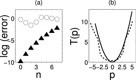
Figure 2: (a) Error in the lowest 8 eigenvalues of the harmonic oscillator. vN($\circ$), pvN($\blacktriangle$). (b) Kinetic energy spectra using 16 basis functions. vN(dashed), pvN(solid).

In the bvN basis set we are able to remove some of the basis functions and construct lower dimensional $H^{\rm bvN}$ and $S^{\rm bvN}$ matrices without losing accuracy. In order to test this claim, we calculated numerically the eigenenergies of the Morse oscillator $V(x)=D(1-e^{-\beta x})^{2}$ and the Coulomb potential $V(x)=-\frac{Q^{2}}{x}$ by using both the FGH and fvN basis sets. The Morse parameters were taken to be $D=12$, $m=6$, $\beta=0.5$ and $\hbar=1$. For FGH, 100 grid points between $[-1.6,20.1]$ were required in order to get 4 digits of accuracy in energy for all 24 bound states. By using the bvN basis functions (constructed from 10$\times$10 vN functions with $\alpha=0.5$) we obtain the same 4 digit accuracy with only 48 basis functions. This is demonstrated graphically in Fig. 3 (a). The figure shows the phase space representation of 100 evenly grid points. Although it requires 100 pvN basis functions to span this area in phase space, due to the flexibility of the bvN basis set we can suffice with just the basis functions in the classically allowed region (white squares).

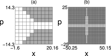
Figure 3: Phase space area spanned in the bvN method (white) and in the pvN (or FGH) method (full rectangle) for Morse (a) and Coulomb (b).

In the Coulomb potential the efficiency of the bvN basis set is even higher. The rectangular shape in phase space of the FGH is a very wasteful representation for the cross-like shape of the eigenstates. The Coulomb parameters were taken to be $Q=1$, $m=1$ and $\hbar=0.5$. For FGH 1599 grid points between $[-50.2,50.1]$ were required in order to get 4 digits of accuracy in energy for the first 9 excited states. By using the bvN basis functions (constructed from 39$\times$41 vN functions with $\alpha=0.2367$) only in the classically allowed energy shell we obtain the same accuracy with only 189 basis functions. Fig. 3 (b)illustrates the efficiency of the bvN basis by showing the phase space area in FGH and bvN bases. Figure 4 shows the error in the eigenenergies by using 190 functions in the FGH and in the bvN method respectively.

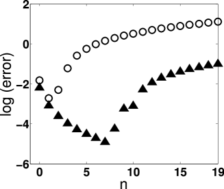
Figure 4: The deviation between the calculated and the exact eigenenergies for the lowest 20 eigenstates of the Coulomb potential using 190 basis functions for the bvN ($\blacktriangle$) and pvN (or FGH)($\circ$)

The ability to localize a bvN function at a specific point in phase space results in the remarkable concept of 1 basis function per 1 eigenstate. This means that in order to calculate $N$ eigenenergies we need only $N$ basis functions. Obviously, such one per one efficiency, if reachable, will be the ideal efficiency for any basis set. In order to test the ability of the bvN method to reach the ideal efficiency we examined the Morse potential and looked for the smallest number of bases that will provide exact values of the energies (12 digits of accuracy) for all the eigenstates in the energy shell $E=11.25$. The bvN method indeed, tends to the ideal efficiency in the classical limit where $\hbar\rightarrow 0$ (Fig. 5). This remarkable result is unique for the bvN method. For example, the efficiency of the Fourier method has an upper bound, which can be calculated analytically as $\eta=1.6959$ (the ratio of the classically allowed phase space to the area of the rectangle).

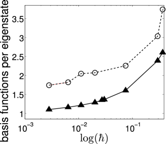
Figure 5: Basis efficiency for the Morse potential as function of $\hbar$. For pvN (or FGH) (dashed) and bvN(solid)

In summary, we introduced the “Gaussian-like” pvN basis set and showed the equivalence between the pvN and the Fourier method. Several TISE problems were tested. We showed that the pvN method is as accurate as the Fourier method; however, due to the localization of the basis functions, we can construct a flexible basis set, bvN, which is much more efficient then the FGH. We also have shown that in the classical limit the number of basis functions is equal to the number of the exact eigenvalues. This remarkable “1 per 1” quality, is of course, an optimal result for any basis set, and as far as we are aware has never been achieved before.

As discussed above, the use of primitive Gaussian functions on the vN lattice yields disappointing results davis_and_heller ; poirier . The success of our method is due to two key points: 1. By defining the basis set as a linear combination of the $\{\theta_{i}(x)\}$ we ensure that the basis indeed spans a band limited region with finite support. 2. By using the bvN basis set the coefficients become locallized. In the conventional Gaussian basis set the delocalized coefficients arise from the non-locality of $S^{-1}$.

In this paper we focused on model 1-d TISE problems. However, Gaussians are used as basis functions in a variety of methods for solving the TISE and TDSEhk ; shalashilin ; fg ; martinez . All these methods have suffered from numerical difficulties resulting from the non-locality of $S^{-1}$ and we believe that significant improvement is possible using the pvN and the bvN basis sets. Finally, the pvN method is not limited to quantum mechanical problems. There is a large literature on the use of a Gaussian basis set in signal processing where it goes by the name of the Gabor transform gabor ; bastians ; ingrid ; orr ; porat . The Gabor transform is known to have problems with stability, which can be traced to the “no-go” theorem of Balian and Lowbalian ; low —the statement that localized basis sets are incompatible with orthogonal basis sets. While the pvN and bvN bases do not violate the no-go theorem, they seem to effectively circumvent it. We therefore believe they can have a significant impact on signal processing in general.

This work was supported by the Israel Science Foundation and made possible in part by the historic generosity of the Harold Perlman family.

References

- (1) R.Kosloff in Numerical Grid Methods and their Application to Schrödinger’s Equation ed. C. Cerjan (Kluwer, Boston, 1993)
- (2) C. C. Marston and G. G. Balint-Kurti, J.Chem.Phys. 6, 3571 (1989).
- (3) G. W. Wei, J.Phys.B. 33, 343 (2000)
- (4) Z.Bačić, R.M Whitnell, D.Brown and J.C.Light, Comp. Phys. Comm. 51, 35 (1988)
- (5) S. Garashchuk and J. C.Light, J.Chem. Phys. 114, 3929 (2001)
- (6) E. T. Whittaker, Proc. R. Soc. Edinburgh 35, 181 (1915).
- (7) H. Nyquist, Trans. AIEE 1 47, 617 (1928).
- (8) C. E. Shannon, Proc. IRE 37, 10 (1949).
- (9) S. Fechner, F. Dimler, T. Brixner, G. Gerber and D. J.Tannor, Opt. Express 15, 15389 (2007)
- (10) J.von Neumann, Math. Ann. 104, 570 (1931)
- (11) A.M Perelomov, Theor. Math.Phys 11, 156 (1971)
- (12) M.J.Davis and E J.Heller, J.Chem. Phys. 71, 3383 (1979)
- (13) B. Poirier and A.Salam, J.Chem. Phys. 121, 1690 (2004)
- (14) F. Dimler, S. Fechner, A. Rodenberg, T. Brixner, and D. J.Tannor, New J. of Phys. 11, 105052 (2009)
- (15) D. J. Tannor, Introduction to Quantum Mechanics: A Time-dependent Perspective (University Science Books, Sausalito, 2007), eq.11.163.
- (16) Ref.tannor_book eq.11.172.
- (17) E. Fattal, R. Baer and R. Kosloff, Phys. Rev. E. 53, 1217 (1996)
- (18) M. F. Herman and E. Kluk, J.Chem. Phys. 91, 27 (1984)
- (19) D. V. Shalashilin and M. S. Child, J.Chem. Phys. 113, 10028 (2000)
- (20) E J.Heller, J.Chem. Phys. 75, 2923 (1981)
- (21) M. Ben-Nun and T. J.Martinez, J.Chem. Phys. 108, 7244 (1998)
- (22) D.Gabor, J. Inst. Elect. Eng. 93, 429 (1946)
- (23) M.J.Bastiaans, IEEE 68, 538 (1980)
- (24) I. Daubechies, IEEE 36, 961 (1990)
- (25) R. S.Orr, Signal Processing 34, 85 (1993)
- (26) T. Genossar and M. Porat, IEEE 22, 449 (1992)
- (27) R. Balian, C. R. Acad. Sci. III 292, 1357 (1981)
- (28) F. Low, in A Passion for Physics–Essays in Honor of Geoffrey Chew (World Scientific, Singapore, 1985), pp.17-22