Nonlinear response of dense colloidal suspensions under oscillatory shear: Mode-coupling theory and FT-rheology experiments

Abstract

Using a combination of theory, experiment and simulation we investigate the nonlinear response of dense colloidal suspensions to large amplitude oscillatory shear flow. The time-dependent stress response is calculated using a recently developed schematic mode-coupling-type theory describing colloidal suspensions under externally applied flow. For finite strain amplitudes the theory generates a nonlinear response, characterized by significant higher harmonic contributions. An important feature of the theory is the prediction of an ideal glass transition at sufficiently strong coupling, which is accompanied by the discontinuous appearance of a dynamic yield stress. For the oscillatory shear flow under consideration we find that the yield stress plays an important role in determining the non linearity of the time-dependent stress response. Our theoretical findings are strongly supported by both large amplitude oscillatory (LAOS) experiments (with FT-rheology analysis) on suspensions of thermosensitive core-shell particles dispersed in water and Brownian dynamics simulations performed on a two-dimensional binary hard-disc mixture. In particular, theory predicts nontrivial values of the exponents governing the final decay of the storage and loss moduli as a function of strain amplitude which are in excellent agreement with both simulation and experiment. A consistent set of parameters in the presented schematic model achieves to jointly describe linear moduli, nonlinear flow curves and large amplitude oscillatory spectroscopy.

I Introduction

A standard method to probe the viscoelastic character of a material is to measure the time dependent stress response to an externally applied oscillatory shear field larson1 . The simplicity of oscillatory shearing experiments presents distinct practical advantages when compared to other flow protocols and thus makes desirable a systematic method for the rheological characterization of a material on the basis of the periodic stress response alone. For small strain amplitudes the shear stress is a simple harmonic function, oscillating with the fundamental frequency dictated by the applied strain field. The details of the microscopic interactions underlying the macroscopic stress response are encoded in the familiar storage ($G^{\prime}$) and loss ($G^{\prime\prime}$) moduli of linear response. General aspects of the viscoelastic character of the material can thus be inferred from the magnitudes of the moduli as a function of frequency.

While, for many systems of interest, the linear response regime is well understood, for practical applications, such as the production and processing of materials in industry coussot , it is necessary to consider deformations of finite, often large, amplitude. In the nonlinear regime, the stress response to a sinusoidal excitation contains higher harmonic contributions, which arise from the nonlinearity of the underlying constitutive relation expressing the stress as a functional of the strain larson2 ; wilhelm1 ; wilhelm2 . For many complex materials, consideration of the fundamental frequency alone proves insufficient for describing the physical mechanisms at work for finite strain amplitude. Analysis based purely on the linear complex modulus as a function of frequency can thus be expected to give only a partial mechanical characterization of the system under study (see e.g. mckinley ; mckinley_preprint ). This failing is found to be particularly pronounced for yield stress materials such as aqueous foams fielding and, as we will argue in the present work, colloidal suspensions close to, or beyond, the point of dynamical arrest. Although such systems are predominately elastic in character, they exhibit a complex transient response to oscillatory shear in which the viscous dissipation mechanism present at small strain amplitudes crosses over to a plastic flow as the amplitude is increased. The nonlinear stress response reflecting the onset of plastic flow gives rise to a strong increase in the amplitudes of the higher harmonics.

The emerging discipline of Fourier transform rheology (FT-rheology), originating in the work of Wilhelm and co-workers (see, e.g. wilhelm1 ; wilhelm2 ; Wilhelm07 ; wilhelm_99 ), aims to quantify the nonlinear response of complex fluids by analyzing the harmonic structure of the stress signal measured in large amplitude oscillatory shear (LAOS) experiments (for recent developments see rogers ). Despite considerable progress on the experimental side, the theoretical description of the nonlinear regime remains unsatisfactory. Theoretical treatments capable of capturing higher harmonic contributions have been largely restricted to phenomenological models based on the ideas of continuum rheology larson2 ; mckinley_preprint ; Wilhelm07 ; cho ; hassager ; noll . A more refined description of the nonlinear response is provided by mesoscopic models in which the time evolution of explicit coarse-grained degrees of freedom is governed by specified dynamical rules mes1 ; mes4 ; derec . While such approaches are capable of capturing generic features of the response, they are not material specific and make no explicit reference to the underlying particle interactions.

Recently, progress in making the connection between microscopic and macroscopic levels of description has been made for the case of dense colloidal suspensions subject to time-dependent flow joeprl_07 ; joeprl_08 . The developments in classical nonequilibrium statistical mechanics presented in joeprl_07 and joeprl_08 extend earlier work focused on the simpler, but fundamental, case of steady shear flow fuchs_cates_PRL ; fc_jrheol . The mode-coupling-type approximations employed in joeprl_07 ; joeprl_08 ; fuchs_cates_PRL ; fc_jrheol capture the slow structural relaxation leading to dynamical arrest in strongly coupled systems (i.e. dispersions at high volume fraction or with a strongly attractive potential interaction), with the consequence that the macroscopic flow curves $\sigma(\dot{\gamma})$ attain a finite value in the limit of vanishing rate, for states which would be glasses or gels in the absence of flow. The finite value of the stress in the slow flow limit identifies the dynamic yield stress. The relationship between the dynamic yield stress and its more familiar static counterpart is analogous to that between stick and slip friction in engineering applications. A prediction of particular importance made by the the MCT-based approaches of joeprl_07 ; joeprl_08 ; fuchs_cates_PRL ; fc_jrheol is that the dynamic yield stress appears discontinuously as a function of coupling strength, in clear contrast to mesoscopic models mes1 ; mes4 which predict a continuous power law dependence. The notion of yield stress was considered in a more general and abstract sense in pnas , in which a dynamic yield stress surface, describing yielding under more general non-shear deformations, was calculated (see also joe_review ).

Although the closed, microscopic constitutive equation presented in joeprl_08 is of considerable generality, the combined difficulties of a large time-scale separation between microscopic and structural relaxation times, spatial anisotropy, and lack of time-translational invariance presented by many problems of interest makes direct numerical solution of the equations impossible at the present time. In order to both facilitate numerical calculations and expose more transparently the essential physics captured by the fully microscopic theory of joeprl_08 a simplified ‘schematic’ model has been proposed pnas . Schematic models have proved invaluable in the analysis and assessment of microscopic mode-coupling approaches, both for quiescent systems MCTequations and under steady shear flow faraday , in each case providing a simpler set of equations which aim to retain the essential mathematical structure of the fully microscopic theory. While the schematic model reduction performed in pnas leads to loss of the ‘first principles’ character of the approach, the mathematical connections between full and schematic theory nevertheless serve to elevate the schematic model above purely phenomenological approaches.

In the present work we will consider application of the schematic model derived in pnas to the problem of large amplitude oscillatory shear. Although the tensorial schematic model of pnas is closely related to the earlier $F_{12}^{\dot{\gamma}}$ model derived in faraday , application of the tensorial model to a simple shear flow geometry does not exactly reproduce the $F_{12}^{\dot{\gamma}}$ model. The study of time-dependent flows, not considered in earlier work, revealed that corrections to the original $F_{12}^{\dot{\gamma}}$ model were necessary to capture correctly the response to rapidly varying flows. The modifications thus introduced lead to small differences in the steady state rheological predictions. Nevertheless, the present schematic models describes the same phenomenology as the previous model hajnal_scaling when applied to steady shear.

Comparison of theoretical predictions with experimental data for thermosensitive core-shell particles, dispersed in water, has been performed using the $F_{12}^{\dot{\gamma}}$ model faraday . These particles have the very convenient feature that the volume fraction of the system may be varied continuously over a considerable range, simply by tuning the temperature of the system. Moreover, the finite polydispersity in particle size effectively suppresses crystallization, such that studies of dense fluid and glassy states are not complicated by an intervening fluid-crystal transition. In a series of works, theory and experiment have been compared for the flow curves under steady shear fuchs_ballauff ; crassous0 and, more recently, for both flow curves and linear response moduli crassous ; winter . A particular strength of the $F_{12}^{\dot{\gamma}}$ model (inherited by the more recent model of pnas ) is that both flow curves and linear viscoelastic moduli can be simultaneously and accurately fitted over many decades of shear rate and frequency, respectively, using a consistent and physically meaningful set of fit parameters. In winter a combination of experimental techniques were employed, which enabled measurement of the flow curves and linear response moduli over eight and nine orders of magnitude in shear rate and frequency, respectively winter . Although certain discrepancies between experiment and theory at low frequencies remain to be fully understood, the general level of agreement is impressive. Reassuringly for the schematic models, the complete microscopic MCT calculations possible for the linear response moduli agree with the data from the monodisperse samples on the $40$% error level crassous0 .

The nonlinear rheology of thermosensitive microgel particles (identical to those considered in the present work) was addressed in a recent experimental study, focused on the stress response to steady and large amplitude oscillatory flow carrier . In addition to a study of the stress overshoot following the onset of shear flow (see also zausch ), both the strain dependence of the storage and loss moduli and the higher harmonic contributions were analyzed. Despite employing the same thermosensitive particles and LAOS flow protocol, the study carrier should be regarded as complementary to the present work. In carrier volume fractions well above random close packing were investigated ($\phi>0.64$), suggesting considerable deformation of the particles themselves, whereas we focus here on packing fractions around the glass transition. Moreover, emphasis in the present work is placed on assessing the MCT based schematic theory presented in pnas for a nontrivial flow history, namely large amplitude oscillatory shear, and comparison of the theoretical predictions with experiment. This comparison provides the first truly time-dependent test of this recently developed schematic model beyond the simple case of step strain already considered in pnas .

The paper will be organized as follows: In Section II we summarize the microscopic starting points underlying our theoretical approach, before proceeding to give a compact overview of the linear and nonlinear response of viscoelastic systems, relevant for the subsequent analysis. In Section III we introduce the schematic MCT model and discuss its relation to previous work. In Section IV we discuss the Brownian dynamics simulation algorithm used to generate results supplementary to those of theory and experiment. Section V contains the experimental details. In Section VI we first present purely theoretical results, in order to establish the phenomenology predicted by the schematic model. We then consider the results of our two-dimensional simulations before proceeding to analyze and fit the experimental data. Finally, in Section VII we discuss the significance of the present work and provide an outlook for future studies.

II Fundamentals

II.1 Microscopic starting points

The shear stress resulting from a general time-dependent shear strain of rate $\dot{\gamma}(t)$ is given by a generalized Green-Kubo relation joeprl_07 ; joeprl_08

$$\sigma(t)=\int_{-\infty}^{\,t}\!\!dt^{\prime}\;\dot{\gamma}(t^{\prime})\,G(t,t^{\prime}).$$ (1)

Equation (1) is nonlinear in the shear rate due to the nonlinear functional dependence of the shear modulus $G(t,t^{\prime})$ on $\dot{\gamma}(t)$. Within the microscopic framework developed in joeprl_07 ; joeprl_08 the modulus is identified as the correlation function of fluctuating stresses

$$G(t,t^{\prime})=\frac{1}{k_{B}TV}\langle\,\hat{\sigma}_{xy}e_{-}^{\int_{t^{\prime}}^{t}ds\Omega^{\dagger}(s)}\,\hat{\sigma}_{xy}\,\rangle,$$ (2)

where $\hat{\sigma}_{\rm xy}\!\equiv\!-\sum_{i}\,F_{i}^{\rm x}y_{i}$ is a fluctuating stress tensor element, formed by a weighted sum of the forces acting on the particles for a given configuration, $T$ is the temperature, $V$ is the system volume and $\langle\cdot\rangle$ indicates an equilibrium average. The particle dynamics to be considered in the present work are generated by the adjoint Smoluchowski operator dhont

$$\Omega^{\dagger}(t)=\sum_{i}D_{0}\,[\,\bm{\partial}_{i}+\beta{\bf F}_{i}\,]\cdot\bm{\partial}_{i}+D_{0}\dot{\gamma}(t)y_{i}\frac{\partial}{\partial x}$$ (3)

where $\beta=1/k_{B}T$ and $D_{0}$ is the short time diffusion coefficient at infinite dilution. The time-ordered exponential function in Eq.(2) arises because $\Omega^{\dagger}(t)$ does not commute with itself for different times vankampen .

An important approximation underlying Eq.(3) (and thus (2)) is that solvent induced hydrodynamic interactions (HI) between the colloidal particles are neglected. The diffusion coefficient entering Eq.(3) is thus a scalar quantity and the external flow may be included using a prescribed (as opposed to self-consistently calculated) shear field $\dot{\gamma}(t)$. While the omission of HI may be inappropriate at high shear rates, for which hydrodynamically induced shear thickening can occur in certain systems, it is expected to represent a reasonable approximation for slowly sheared states close to the glass transition. Nevertheless, when attempting to fit experimental data using theoretical models based on Eq.(3) it proves neccessary to include an empirical hydrodynamic correction accounting for the high frequency viscosity. In addition to the neglect of HI we make two, potentially more dangerous, assumptions: (i) $\dot{\gamma}(t)$ is taken to be spatially translationally invariant, which may become questionable when considering the flow response of dynamically arrested states. (ii) The shear field acts instantaneously. While this should be acceptable for certain flow histories the general status of this approximation is not clear.

II.2 Linear response

Following standard convention, we consider an externally applied shear strain of the form

$$\gamma(t)=\gamma_{0}\sin(\omega t).$$ (4)

The time translational invariance of the shear field (4) gives rise to an explicit dependence of the modulus (2) upon two time arguments.

For small deformation amplitudes ($\gamma_{0}\ll 1$) the strain dependence of the shear modulus may be neglected, such that Eq.(1) provides a linear relationship between $\dot{\gamma}(t)$ and $\sigma(t)$. This leads to the approximation

$$G(t,t^{\prime})=G_{\rm eq}(t-t^{\prime}),$$ (5)

where $G_{\rm eq}(t)$ denotes the time translationally invariant equilibrium shear modulus. Substitution of (4) and (5) into Eq.(1) and employing trigonometric addition formulas leads directly to the familiar linear response result

$$\sigma(t)=\gamma_{0}G^{\prime}(\omega)\sin(\omega t)+\gamma_{0}G^{\prime\prime}(\omega)\cos(\omega t),$$ (6)

where $G^{\prime}(\omega)$ and $G^{\prime\prime}(\omega)$ are the storage and loss moduli, respectively, defined by

$$G^{\prime}(\omega) = \omega\!\int_{0}^{\infty}\!\!dt^{\prime}\sin(\omega t^{\prime})\,G_{\rm eq}(t^{\prime})$$ (7)

$$G^{\prime\prime}(\omega) = \omega\!\int_{0}^{\infty}\!\!dt^{\prime}\cos(\omega t^{\prime})\,G_{\rm eq}(t^{\prime}).$$ (8)

Furthermore, Eq.(6) can be rewritten as

$$\sigma(t)=\gamma_{0}|G(\omega)|\sin\left(\omega t+\delta(\omega)\right),$$ (9)

where the complex modulus is given by $G=G^{\prime}+iG^{\prime\prime}$ and the phase shift by $\delta=\arctan(G^{\prime\prime}/G^{\prime})$. If $G^{\prime\prime}(\omega)=0$ the response is purely elastic, in phase with $\gamma(t)$ ($\delta=0$). In the case $G^{\prime}(\omega)=0$ dissipation dominates and the response is in phase with $\dot{\gamma}(t)$ ($\delta=90^{\circ}$).

II.3 Nonlinear response

It should be clear at this stage that the familiar linear response form (6) is a direct consequence of the convolution integral which results from inserting the time translationally invariant equilibrium function (5) into Eq.(2). For finite strain amplitudes, the dependence of the modulus upon two time arguments prevents the simple trigonometric manipulations leading to Eq.(6). Nevertheless, the non-sinusoidal stress response, $\sigma(t)$, is periodic with period $2\pi/\omega$, and may therefore be expressed as a Fourier series

$$\sigma(t)=\gamma_{0}\sum_{n=1}^{\infty}G^{\prime}_{n}(\omega)\sin(n\omega t)+\gamma_{0}\sum_{n=0}^{\infty}G^{\prime\prime}_{n}(\omega)\cos(n\omega t),$$

(10)

where $G^{\prime}_{n}$ and $G^{\prime\prime}_{n}$ are frequency dependent Fourier coefficients given by boas

$$G^{\prime}_{n}(\omega)=\frac{\omega}{\pi}\int_{-\pi/\omega}^{\pi/\omega}\!dt\;\sigma(t)\sin(n\omega t)$$ (11)

$$G^{\prime\prime}_{n}(\omega)=\frac{\omega}{\pi}\int_{-\pi/\omega}^{\pi/\omega}\!dt\;\sigma(t)\cos(n\omega t).$$ (12)

In the limit $\gamma_{0}\rightarrow 0$ the coefficients $G^{\prime}_{1}$ and $G^{\prime\prime}_{1}$ reduce to the familiar linear response moduli. It should be noted that we retain the $n=0$ term in the second sum of (10) in order to leave open the possibility of a stress offset.

Employing manipulations analogous to those leading from (6) to (9) the Fourier series (10) may be expressed in the form

$$\sigma(t)=\gamma_{0}\sum_{n=1}^{\infty}I_{n}(\omega)\sin(n\omega t+\delta_{n}(\omega)),$$ (13)

where the amplitude is given by $I_{n}=|G^{\prime}_{n}+iG^{\prime\prime}_{n}|$ and the phase shifts by $\delta_{n}(\omega)=\arctan(G_{n}^{\prime\prime}/G_{n}^{\prime})$. In analyzing our theoretical, experimental and simulation results we will focus on the behaviour of both the generalized moduli $G^{\prime}_{n}$ and $G^{\prime\prime}_{n}$ and the amplitude and phase shift, $I_{n}$ and $\delta_{n}$, of the fundamental ($n=1$) and higher harmonics ($n>1$) as a function of the control parameters.

Following a period of transient response after initiation of the strain field (switching on the rheometer) the system enters a stationary state, demonstrating a periodic stress response. Although, to some extent, an issue of semantics, it is important that the ‘stationary’ state presently under consideration be distinguished from ‘steady’ states, of the kind achievable by application of a time-independent shear flow. The stationary state is simply a well characterized and periodic transient and is thus influenced by additional physical mechanisms (e.g. thixotropy) which are irrelevant for steady states. In a physical system the stationary response must be independent of the direction of shear, leading to a stress $\sigma(t)$ symmetric in $\dot{\gamma}(t)$. The mirror symmetry of the constitutive equation has the consequence that only odd terms contribute to the Fourier series (13). The appearance of even harmonics in the analysis of experimental data is often an indication of boundary effects, such as wall slip, or other inhomogeneities of the flow Wilhelm07 .

Important physical interpretation may be given to the coefficient $G^{\prime\prime}_{1}$ by considering the energy dissipated per unit volume of material per oscillation cycle

$$E_{d}=\int_{-\pi/\omega}^{\pi/\omega}\!dt\;\sigma(t)\dot{\gamma}(t).$$ (14)

Substitution of the strain field (4) and the Fourier series (10) into Eq.(14) leads to

$$E_{d}=\gamma_{0}^{2}\pi\,G^{\prime\prime}_{1}(\omega),$$ (15)

(see also hyun_wilhelm ). Thus, for a sinusoidal strain of the form (4), energy is dissipated only at the input frequency. The coefficient $G^{\prime\prime}_{1}$ therefore has the same interpretation in the non-linear regime as in the linear regime: it determines the dissipation of energy over an oscillation cycle. The remaining coefficients in the series, $G^{\prime}_{n}$ and $G^{\prime\prime}_{n>1}$, thus collectively describe the reversible storage and recovery of elastic energy.

II.4 Lissajous plots

A standard way to graphically represent the relationship between $\gamma(t)$ and $\sigma(t)$ is via the Lissajous representation, in which trajectories are shown in the $\gamma^{*},\sigma^{*}$ plane, where $\gamma^{*}=\gamma/\gamma_{\rm max}$ and $\sigma^{*}=\sigma/\sigma_{\rm max}$ are the strain and stress, normalized by their maximum values lissajous_old . In this representation, a general linear viscoelastic response is characterized by an ellipse, symmetric about the line $\gamma^{*}=\sigma^{*}$, point symmetric with respect to the origin plus two mirror planes. The two limiting cases of a purely elastic and a purely dissipative response are thus characterized by a line and a circle, respectively. In the nonlinear regime considerable deviations from ellipticity are observed. The specific character of these deviations can indicate whether a material is, for example, strain hardening or strain softening (an increase/decrease of $G^{\prime}$ with strain amplitude), and thus provides a useful, albeit qualitative, ’rheological fingerprint‘ of a given material mckinley ; mckinley_preprint . For a general nonlinear response, the area enclosed within the closed loop trajectory of a Lissajous figure is directly related to the dissipated energy via the integral in Eq.(14). This lends an appealing physical interpretation to the Lissajous representation and provides a direct visual impression of the dissipative character of the response.

III Theoretical approach

III.1 Schematic model

As noted in the introduction, the approximate microscopic constitutive theory developed in joeprl_07 ; joeprl_08 enables first-principles prediction of the rheological behaviour of dense colloidal dispersions. However, the simultaneous occurrence of spatial anisotropy and non-time translational invariance hinders numerical solution of the equations when addressing concrete problems. The schematic model presented in pnas provides a simplified set of equations which, it is hoped, capture the essential physics contained within the full equations, while remaining tractable for numerical implementation.

Within the schematic reduction, the modulus is expressed in terms of a single-mode transient density correlator

$$G(t,t^{\prime})=v_{\sigma}\Phi^{2}(t,t^{\prime})$$ (16)

where $v_{\sigma}$ is a parameter measuring the strength of stress fluctuations. The approximation underlying (16) is that stress fluctuations relax as a result of relaxations in the density (viz. structural relaxation). The assumption that $v_{\sigma}$ is independent of strain is a simplifying assumption which could be relaxed if neccessary. The microscopic theory of joeprl_08 predicts both the temporal and wavevector dependence of the transient density correlater under applied flow. The schematic, single mode, density correlator (normalized to $\Phi(t,t)=1$) represents, in some non-specific sense, a ‘typical’ correlator of the microscopic theory. It is obtained from solution of a nonlinear integro-differential equation

$$\dot{\Phi}(t,t^{\prime})+\Gamma\bigg{(}\Phi(t,t^{\prime})+\int_{t^{\prime}}^{t}ds\,m(t,s,t^{\prime})\dot{\Phi}(s,t^{\prime})\bigg{)}=0.$$

The single decay rate $\Gamma$ sets the time-scale and would, within a microscopically based theory, depend upon both structural and hydrodynamic correlations. The overdots in Eq.(III.1) imply differentiation with respect to the first time argument. The memory function $m(t,s,t^{\prime})$ appears in Eq.(III.1) as a generalized friction kernel, which can be formally identified as the correlation function of certain stress fluctuations. Making the assumption that these stress fluctuations may be expressed in terms of density fluctuations (both become slow close to the glass transition) leads to a tractable expression for $m(t,s,t^{\prime})$ as a quadratic functional of the transient density correlator and, thus, a closed theory. A somewhat surprising consequence of the formal calculations presented in joeprl_07 ; joeprl_08 is that the memory function possesses three time arguments. The presence of a third time argument, which would have been difficult to anticipate on the basis of quiescent MCT intuition, has important consequences for rapidly varying flows (e.g. step strain joeprl_07 ). Within the schematic model the memory function is given by

$$m(t,s,t^{\prime})=h(t,t^{\prime})\,h(t,s)\,[\,\nu_{1}\Phi(t,s)+\nu_{2}\Phi^{2}(t,s)\,].$$

Following conventional MCT practice the parameters $\nu_{1}$ and $\nu_{2}$ represent, in an unspecified way, the role of the static structure factor in the microscopic theory and are chosen as $v_{2}=2$ and $v_{1}=2(\sqrt{2}-1)+\epsilon/(\sqrt{2}-1)$. The separation parameter $\epsilon$ is a crucial parameter within our approach and encodes the thermodynamic statepoint of the system by measuring the distance from the glass transition. Negative values of $\epsilon$ correspond to fluid states and positive values to glass states. Setting $h$ equal to unity in Eq.(III.1) recovers the well known $F_{12}$ model, originally introduced by Götze MCTequations ; goetze_zeit ; sjoegren . The linear term in $\Phi$ which appears in Eq.(III.1) is absent from the microscopic mode-coupling expression, but turns out to be necessary for a faithful reproduction of its asymptotic properties within a single-mode theory. Under simple shear flow, the $h$-functions in the memory kernel (III.1) serve to accelerate the loss of memory caused by the affine advection of density fluctuations. The assumption that the same function $h$ may be used to incorporate both the strain accumulated between $t$ and $t^{\prime}$ as well as that between $t$ and $s$ is an approximation, made to keep the theory as simple as possible. Taking account of the required invariance with respect to flow direction suggests the simple ansatz

$$h(t,t^{\prime})=\frac{\gamma_{c}^{2}}{\gamma_{c}^{2}+\gamma^{2}},$$ (19)

where $\gamma\equiv\gamma(t,t^{\prime})=\int_{t^{\prime}}^{t}ds\,\dot{\gamma}(s)$ and the parameter $\gamma_{c}$ sets the scale of strain.

Eq.(1) and (16)-(19) provide a closed constitutive theory which depends upon three adjustable parameters $(v_{\sigma},\Gamma,\gamma_{c})$ and two control parameters $(\epsilon,\dot{\gamma})$ representing the coupling strength and applied shear rate. As the schematic model under discussion is implicitly based on the Smoluchowski dynamics described by Eq.(3), the influence of HI is neglected. While this is not important for capturing correctly the qualitative features of the rheological response, quantitative comparison requires a simple hydrodynamic correction at high frequencies. The simplest approximation, which we will employ in the present work, is to empirically add an extra term to the shear modulus

$$G(t,t^{\prime})\rightarrow G(t,t^{\prime})+\eta_{\infty}\,\delta(t-t^{\prime}).$$ (20)

The high frequency viscosity, $\eta_{\infty}$, is thus introduced into the model, describing the viscous processes which occur on timescales much shorter than the structural relaxation time. The correction (20) has the consequence that the stress acquires an extra term, linear in $\dot{\gamma}$, and the Fourier coefficient $G^{\prime\prime}_{1}$ is shifted by a term linear in $\omega$.

III.2 Strain-rate frequency superposition

An alternative mode-coupling-type approach, describing the collective density fluctuations of dense colloidal fluids under shear, is provided by the work of Miyazaki et al. miyazaki1 ; miyazaki2 ; miyazaki3 . By considering time-dependent fluctuations about the steady state a closed (scalar) constitutive equation has been derived and applied to colloidal dispersions in two-dimensions under steady shear miyazaki1 ; miyazaki2 and in three dimensions (subject to additional isotropic approximations) under large amplitude oscillatory shear miyazaki3 . Given the very different nature of the approximations underlying the present MCT-based theory joeprl_07 ; joeprl_08 ; fuchs_cates_PRL ; fc_jrheol and that of miyazaki1 ; miyazaki2 ; miyazaki3 (fluctuating hydrodynamics vs. projection operator methods) it is interesting that the final expressions (e.g. the memory function vertices entering the equation of motion for the transient correlator) are rather similar, at least for the special case of steady shear. For the case of large amplitude oscillatory shear, however, the theory presented in miyazaki3 differs clearly and fundamentally from the microscopic approaches to time-dependent shear developed in joeprl_07 ; joeprl_08 and, consequently, from the schematic model of pnas to be employed in the present work. The theoretical developments of Miyazaki et al. miyazaki3 motivated the authors to propose the principle of ‘strain-rate frequency superposition’ as a probe of structural relaxation in soft materials wyss .

The essence of the Miyazaki et al. approach can be captured by a simple schematic model, which we will elaborate upon below. In miyazaki3 the authors took the theory which they had developed for steady shear flow miyazaki1 ; miyazaki2 and replaced the steady shear rate $\dot{\gamma}$ appearing in the equation of motion for the correlator, by the time-dependent shear rate $\dot{\gamma}(t)=\gamma_{0}\omega\cos(\omega t)$, describing oscillatory flow. This rather ad hoc treatment gives rise to equations with a mathematical structure appropriate for steady flows and ignores the more realistic, although more complicated, history dependence of theories developed to treat non-steady flows specifically joeprl_07 ; joeprl_08 . On the basis of the results obtained for the strain amplitude dependence of the storage and loss moduli (notated as $G^{\prime}_{1},G^{\prime\prime}_{1}$ in the present work) it was argued that the time-dependence of the strain-rate field $\dot{\gamma}(t)=\gamma_{0}\omega\cos(\omega t)$ is not essential for understanding the viscoelastic response, and that it is sufficient to consider the strain-rate amplitude $\gamma_{0}\omega$ alone. The relevant timescale is thus identified as $(\gamma_{0}\omega)^{-1}$, rather than $\omega^{-1}$. Within the context of schematic mode-coupling equations, this assumption may be expressed by the following memory function

$$m(t)=\frac{[\,\nu_{1}\Phi(t)+\nu_{2}\Phi^{2}(t)\,]}{1+(\gamma_{0}\omega t)^{2}},$$

which, together with the equation of motion

$$\dot{\Phi}(t)+\Gamma\bigg{(}\Phi(t)+\int_{0}^{t}dt^{\prime}\,m(t-t^{\prime})\dot{\Phi}(t^{\prime})\bigg{)}=0,$$

the shear modulus

$$G(t,t^{\prime})=v_{\sigma}\Phi^{2}(t-t^{\prime}),$$ (23)

and Eq.(1) provides a closed theory for $\sigma(t)$. In fact, Eqs.(III.2)-(23) are identical to the $F_{12}^{\dot{\gamma}}$ model MCTequations ; faraday , with a steady shear-rate $\dot{\gamma}=\gamma_{0}\omega$. An important consequence of assuming the dominance of the timescale $(\gamma_{0}\omega)^{-1}$ is that all states, even those which would be glasses in the absence of flow, become fluidized by an applied oscillatory shear field, regardless of the amplitude $\gamma_{0}$. Whether or not a vanishingly small value of $\gamma_{0}$ is really sufficient to restore ergodicity to dynamically arrested states is unclear and presents a fundamental question, with important implications for the existence of a linear response regime.

Despite capturing approximately the amplitude dependence of $G^{\prime}_{1},G^{\prime\prime}_{1}$, describing the response at the fundamental frequency, higher harmonics are ignored in the approach of miyazaki3 . The absence of higher harmonic contributions within the theory of Miyazaki et al. can be traced back to the assumption that the time-dependence of $\dot{\gamma}(t)$ is irrelevant and that this can be represented by the constant $\gamma_{0}\omega$. Within the present context this has the consequence that the memory function (III.2) and correlator, given by solution of (III.2), are constrained to be time-translationally invariant (viz. depend on a single correlation time only). While this assumption is clearly at odds with the underlying variations in the strain field (for which a dependence on the ‘waiting time’ is to be expected), it nevertheless serves to capture first-order corrections to linear response theory, while remaining relatively easy to implement numerically.

The theory developed in miyazaki3 is quasi-linear, in the sense that $\sigma(t)$ remains a simple sinusoid, but with an amplitude and phase shift which depend non-linearly on $\gamma_{0}$. Attempts to justify the neglect of higher harmonics have been based on the fact that the ratio of the third harmonic amplitude to that of the fundamental remains smaller than approximately $20$%, for a wide range of systems miyazaki3 ; wyss . However, in order to draw a fair conclusion, it is important to consider the sum $\sum_{n>1}I_{n}(\omega)/I_{1}$, rather than $I_{3}/I_{1}$ alone, when assessing the physical relevance of higher harmonic contributions. Various experimental studies on colloidal dispersions (see e.g. carrier ) show clearly that the higher harmonics can collectively account for up to half of the total signal, which is not a small effect. This observation serves to emphasize the importance of truly nonlinear theories, which confront directly the non-time translational invariance of the correlation functions, thus going beyond the convolution approximation to Eq.(1).

IV Computer simulation

To provide a point of reference for our theoretical calculations we have performed two-dimensional simulations on a system hard discs undergoing Brownian motion in an external shear field. The simulations are designed to solve approximately the many-body problem of a system of interacting Brownian particles under shear flow. The same Smoluchowski dynamics dhont underlies the microscopic mode coupling theories of joeprl_07 and joeprl_08 which form the basis of the schematic model employed in the present work pnas . We choose to simulate a two-dimensional system for two reasons: (i) The computational resources required are significantly reduced with respect to simulation of three-dimensional systems and thus enables improved statistics to be obtained. (ii) Recent microscopic studies of the quiescent mode-coupling theory in two-dimensions have revealed behaviour broadly similar to that found in three dimensional calculations bayer . We thus expect the reduced dimensionality of our simulation system to be of little consequence for qualitative comparison with the present theory and experimental data.

The basic concept of the algorithm has been described in detail in three dimensions in scala and its adaptation to two dimensions can be found in henrich . We consider a binary mixture of hard discs with the diameters of $D_{s}=1.0$ and $D_{b}=1.4$ with equal particle number concentrations and a total amount of $N=N_{s}+N_{b}=1000$ hard discs in a two-dimensional simulation box of volume $V$ with periodic Lees Edwards boundary conditions. The total two-dimensional volume fraction is then given by $\phi_{tot}=\frac{N\pi}{4V}(D_{b}^{2}+D_{s}^{2})$. We employ this system in order to suppress crystallisation effects. The mass $m$ of the particles and $k_{B}T$ is set equal to unity. We choose our coordinate axes such that flow is in the $x$-direction and the shear gradient is in the $y$-direction. The Brownian timestep was chosen to $\delta t=0.01$ as in henrich . This results in a short time diffusion constant of $D_{0}=0.05$. To implement a time-dependent, oscillatory shear rate, at each Brownian timestep the shear rate is set to its new value

$$\dot{\gamma}(\tau_{B})=\gamma_{0}\,\omega\cos(\omega\tau_{B}),$$ (24)

and all particle velocities are freshly drawn from the Gaussian distribution with $\langle{\bm{v}}^{2}\rangle=2$ and $\langle{\bm{v}}\rangle=\dot{\gamma}(\tau_{B})y(\tau_{B})$. Between two Brownian timesteps the shear rate is kept constant. The strain $\gamma(t)$ can therefore be obtained using

$$\gamma(t)=\sum_{\tau_{B}\in\left[0,t\right]}\dot{\gamma}(t_{B})\delta t\,,$$ (25)

which leads to $\gamma(t)=\int_{0}^{t}{\rm d}t\;\dot{\gamma}(t)$ in the limit of $\delta t\to 0$. At every Brownian timestep the part $\dot{\gamma}(\tau_{B})y(\tau_{B})$ guarantees a linear velocity profile as a linear shear flow is imposed on every particle, depending on its $y$-position. For all simulations the frequency was set to $\omega=0.001$ which leads to Pe${}_{\omega}\equiv\omega D^{2}/4D_{0}=0.05$.

The average quantity of interest in the present work is the time dependent potential part of the shear stress $\sigma_{xy}(t)=\frac{1}{V}\left\langle\sum({\bm{F}}(t)_{ij})_{x}({\bm{r}}(t)_{ij})_{y}\right\rangle$, with the relative force components of particle $i$ and $j$ $({\bm{F}}(t)_{ij})_{x}$ and the particles relative distance component $({\bm{r}}(t)_{ij})_{y}$ for a given time $t$. As we consider hard particles the forces must be calculated from the collision events. By observing the collisions within a certain time window $\Delta\tau_{c}=\left[t_{k},t_{k}+\Delta\tau_{c}\right]$ for a given time $t_{k}$, forces may be extracted using the change of momentum which occurs during the observation time. This leads to the evaluation algorithm for the stress at time $t_{k}$

$$\sigma(t_{k})=\left\langle\frac{1}{\Delta\tau_{c}}\sum_{t_{c}\in\left[t_{k},t_{k}+\Delta\tau_{c}\right]}(\Delta{\bm{v}}(t_{c})_{ij})_{x}({\bm{r}}(t_{c})_{ij})_{y}\right\rangle_{s},\\$$

where summation is over all collisions after time $t_{c}$ within the time window $\Delta\tau_{c}$. The procedure effectively sums the momentum changes $(\Delta{\bm{v}}_{ij})_{x}$ in $x-$ direction multiplied by the relative distance of the particles $({\bm{r}}_{ij})_{y}$ in $y-$ direction. The brackets $\langle...\rangle_{s}$ denote the different simulation runs.
At a total volume fraction of $\phi_{tot}=0.81$ which is slightly above the glass transition for this system (estimated to be at $\varphi=0.79$ on the basis of simulated flow curves henrich ) we prepared $4000$ independent sets for each amplitude $\gamma_{0}\in\{0.001,0.003,0.009,0.01,...,0.09,0.1,0.2,1.0,10.0,100.0\}$ As the system starts from a non stationary state it is necessary to wait for the system to reach it’s long time asymptote (which we found to be the case after undergoing two full oscillations) before meaningful averages can be taken.

V Experiment

V.1 Characterization of the latex particles

The polydisperse latex particles consist of a solid core of poly(styrene) (PS) onto which a thermosentitive network of crosslinked poly(N-isopropylacrylamide) (PNIPAM) is affixed winter . The degree of crosslinking of the shell due to the crosslinker N,N’-methylenebisacrylamide is 2.5 Mol %. As exactly the same particles were used for this work as in winter , the latices have a temperature dependent size (hydrodynamic radius in nm $R_{H}$ = -0.7796 $\cdot$T +102.4096 with T the temperature in ^oC below 25^oC) and a polydispersity of 17% winter . All experiments were done in an aqueous solution of 0.05M KCl to screen residual charges which emerge from the synthesis of the particles. The solid content of the suspension was determined by comparing the weight before and after drying and was found to be 8.35 $wt$%. Neither the MCR 301 measurements nor the FT-rheology measurements at 15.1^∘C lead to a significant change of the solid content (+0.02 $wt$%). However, the FT-rheology measurements at the remaining two temperatures (18.4^∘C and 20^∘C) had a slightly different solid content (9.02 $wt$%) due to the physical relocation of the rheometer to another laboratory and some additional solvent evaporation. The effective volume fraction $\phi_{\rm eff}$ was calculated by using the correlation of mass concentration $c$, hydrodynamic radius and effective volume fraction found in the inset of fig. 6 in winter , which is given by $c\cdot R_{H}^{3}=9.67\cdot 10^{-17}\,g\cdot\phi_{\rm eff}$ for the different temperatures. For the temperature of 15.1^∘C a volume fraction $\phi_{\rm eff}$ of 0.65, for 18.4^∘C a $\phi_{\rm eff}$ of 0.60 and for 20.0^∘C a $\phi_{\rm eff}$ of 0.57 was found. In previous work winter the glass transition for this system was found to be at $\phi_{\rm eff}=0.64$. Given a polydispersity of $17$% the theory of Schärtl and Sillescu sillescu predicts random close packing at $\phi_{\rm eff}=0.68$.

V.2 Rheological Experiments

The rheological experiments cover the range from the linear to the strongly nonlinear regime. The rheological measurements were performed with two instruments a MCR 301 from Anton Paar with a Cone Plate geometry (diameter: 50 mm, cone angle: 0.991^∘) and the FT-rheological measurements with an ARES rheometer (Rheometrics Scientific) with a Cone Plate geometry (diameter: 50 mm, cone angle: 0.04 rad). All measurements were performed after a preshear of 100s^-1 lasting 200s and a waiting time of 10s. For the rheological measurements, a solvent trap (for the ARES instrument equipped with a sponge drawn with water) is used to prevent evaporation. A thin paraffin-layer covers additionally the solution to prevent an exchange with the atmosphere above.
With the MCR 301 the measurements at 15, 18 and 20^∘C were done. The flowcurves were measured from 5$\cdot$10^-4 to 1000s^-1 with a time ramp of 2500s to 20s and then a waiting time of 10s followed by a flowcurve measured from 1000 to 5$\cdot$10^-4s^-1 with a time ramp of 20 to 2500s. For 15^∘C flowcurves in the shear rate range of 1$\cdot$10^-4s^-1 to 1000s^-1 with a timeramp of 10000s to 20s were perfomed. The frequency tests were performed at a deformation of 1% starting from 10Hz to 0.001Hz with a time ramp of 20s to 1000s. All deformation tests were performed with a measurement time for each point of 100s.
For the FT-rheology oscillatory time sweep measurements were performed at the ARES instrument at frequencies of 1, 0.1 and 0.01Hz at different deformation amplitudes. The FT-signal were always recorded after some oscillations, so that the suspension reached the oscillatory stationary state. The first measurements were done at 15.1^∘C and the frequency tests of the ARES and the MCR 301 coincided. For the two higher temperatures the measurements had to be performed for the same ARES instrument at a different room. Here an evaporation effect was observed, so that the temperature had to be adjusted to archieve the same behaviour in the frequency test. Instead of 18${}^{\circ}C$ a temperature of 18.4${}^{\circ}C$ and instead of 20${}^{\circ}C$ a temperature of 20.9${}^{\circ}C$ was used. Typically for the nonlinear FT-rheology measurements with the time sweep tests 40 oscillations for 1 Hz excitation were applied, whereas 10 oscillations for 0.1 Hz and 9 oscillations for 0.01 Hz. To obtain a FT-spectrum from the raw time data we performed a discrete, complex, half-sided fast Fourier transformation bracewell ; wilhelm2 ; wilhelm_99 .

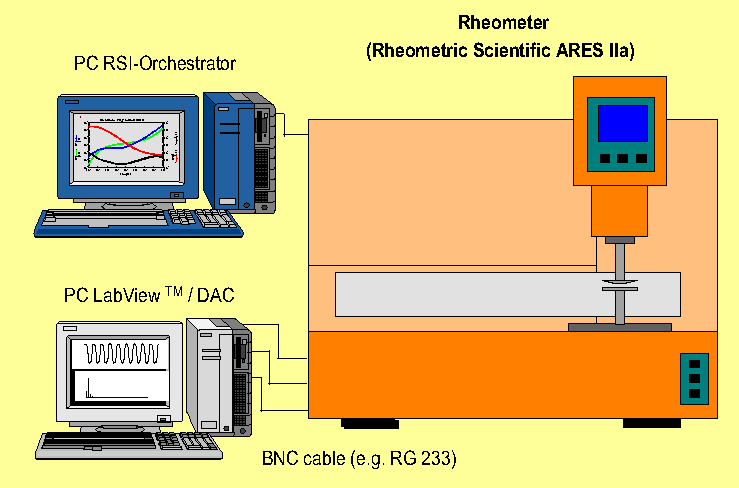
Figure 1: (Experiment) The experimental set-up of FT-rheology with two independent controlling computers, one for normal rheology and one for FT-rheology wilhelm2 .

For further information of the setup, the measuring principal and FT-analysis we would like to refer to klein ; neidhoefer

V.3 Fourier Transform Rheology Apparatus

The FT-rheological setup consists of a Rheometrics Scientific advanced rheometer expansion systems (ARES) and a computer which either controls the rheometer via a serial cable as well as detects the strain and torque force outputs via BNC cables (see Fig.1). The ARES rheometer is a strain-controlled rheometer equipped with a dual range force rebalance transducer (100 FRT) capable of measuring torques ranging from 0.004 mNm to 10 mNm, specified by the manufacturer. It has a high resolution motor, applying frequencies from $10-5$ rad/s to $500$ rad/s and deformation amplitudes ranging from $0.005$ to $500$ mrad. A water bath adjusts the temperature range from $5^{\circ}$C to $95^{\circ}$C. The analog raw data of the measurements are digitized with a $16$-bit ADC. This ADC card has a maximum sampling rate of $50$ kHz per channel. Due to the high sampling rate the time between consecutive data points is very small compared to the timescale of rheological experiments. The loss of information by sampling the torque transducer data is negligible schmidt . To achieve best results with respect to the signal-to-noise ratio, oversampling is applied. The ADC-card acquires the time data at the highest possible sampling rate and then preaverages them on the fly to reduce random noise. With this method the noise is reduced by a factor of 3 to 5 which could only be achieved by averaging multiple measurements dusschoten . Within the set-up a 16-bit ADC card is implemented, which is able to discriminate steps. The quantification resolution of the ADC card limits the ratio. It determines the minimum detectable intensity of weak signals by its ability to discriminate the intensity of the signal. The higher the bit number, the smaller the detectable intensity variation skoog . After acquisition and digitization of the time data, they are handled with Matlab software klein ; neidhoefer .

VI Results

VI.1 Theoretical predictions

VI.1.1 Flow curves

For given values of the parameters ($v_{\sigma},\gamma_{c},\Gamma,\epsilon$) the schematic theory defined by (1) and Eqs.(16)-(19) enables prediction of the flow curve expressing the steady shear stress $\sigma$ as a function of shear-rate $\dot{\gamma}$. Fig.2 shows a set of typical flow curves generated by the schematic MCT model for three fluid states ($\epsilon<0$), the critical state ($\epsilon=0$), and three states in the glass ($\epsilon>0$). The parameters employed for the theoretical calculations presented in Fig.2 (as well as for Figs.3-8) are $v_{\sigma}=100$, $\gamma_{c}=0.15$, $\Gamma=100$ and $\epsilon=10^{-3}$. Experience with fitting the experimental data, to be considered in section VI.3, shows that these choices represent sensible physical values for the model parameters. In the fluid, there exists a linear (Newtonian) regime for small shear-rates ($Pe_{0}\equiv\dot{\gamma}/\Gamma\ll 1$), for which the standard $F_{12}$ model result for the shear viscosity holds, $\sigma=\dot{\gamma}\int_{0}^{\infty}\!dt\,\Phi_{\rm eq}^{2}(t)\equiv\dot{\gamma}\eta$. Increasing the separation parameter to less negative values (corresponding to, e.g. an increase in the volume fraction) gives rise to an increase in $\eta$, reflecting the slowing of the structural relaxation time $\tau$, which dominates all transport properties within our MCT approach. For $\dot{\gamma}\tau>1$ the effect of shear starts to dominate the structural relaxation and the stress increases sub-linearly as a function of shear-rate, corresponding to shear thinning of the viscosity $\eta(\dot{\gamma})=\sigma(\dot{\gamma})/\dot{\gamma}$. At high shear-rates $\dot{\gamma}\tau\gg 1$ the present model yields $\sigma=\dot{\gamma}/\Gamma$ and needs to be supplemented by corrections which account for the high shear limiting viscosity (and which, in the absence of HI, aredetermined by the solvent contribution $\eta_{\infty}$).

As $\epsilon\rightarrow 0^{-}$ the regime of linear response shifts to increasingly lower values of the shear-rate and disappears entirely at the (ideal) glass transition, $\epsilon=0$. For states in the glass there exists a finite stress in the limit of vanishing shear rate, identified as the dynamical yield stress ($\lim_{\dot{\gamma}\rightarrow 0}\sigma(\dot{\gamma})=\sigma_{y}$). Within idealized MCT based treatments the dynamical yield stress emerges discontinuously as $\epsilon$ is varied accross the glass transition (shown in the inset of Fig.2). It should be mentioned that the flow curves shown in Fig.2 differ quantitatively from those of the extensively studied $F_{12}^{\dot{\gamma}}$ model faraday , due to the inclusion of an additional prefactor $h(t,t^{\prime})$ in the expression for the memory function (III.1). Nevertheless, the qualitative predictions of the theory for the flow curves are in full agreement with those of the $F_{12}^{\dot{\gamma}}$ model.

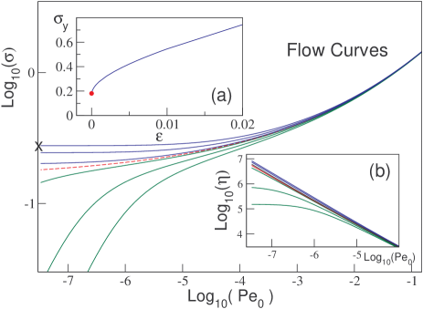
Figure 2: (Theory) The flow curves for fluid states $\epsilon=-10^{-3},-5\times 10^{-4},-10^{-4}$ (green), at the critical point $\epsilon=0$ (red) and for glassy states $\epsilon=10^{-4},5\times 10^{-4},10^{-3}$ (blue). In the glass ($\epsilon>0$) there exists a finite stress in the limit of vanishing shear rate, identified with the dynamical yield stress ($\lim_{\dot{\gamma}\rightarrow 0}=\sigma_{y}$). The cross indicates the yield stress value used in Figs.4 and 5. Inset (a) shows the discontinuous emergence of a dynamical yield stress as a function of $\epsilon$. Inset (b) shows the viscosity $\eta=\sigma/\dot{\gamma}$. Calculations were performed with $\eta_{\infty}=0$.

VI.1.2 Linear response moduli

The linear storage and loss moduli, given by Eqs.(7) and (8), respectively, are shown in Fig.3 as a function of $Pe_{\omega}\equiv\omega/\Gamma$ for two fluid states ($\epsilon<0$) and two glassy states ($\epsilon>0$). In the fluid, the finite value of the structural relaxation timescale $\tau$ is reflected in the maximum of $G^{\prime\prime}$ and the crossing of $G^{\prime}$ and $G^{\prime\prime}$ at low frequency. The fact that $G^{\prime}$ remains notably larger than $G^{\prime\prime}$ at high frequencies is simply a result of neglecting the high frequency limiting viscosity $\eta_{\infty}$ in presenting our theoretical predictions. Setting $\eta_{\infty}=0$ in presenting the theory highlights the contribution of structural processes to the viscoelasticity. In the glass, $G^{\prime\prime}$ goes to zero at low frequencies ($G^{\prime\prime}\!\sim\!\omega$) and $G^{\prime}$ attains a finite low frequency value, identifying the transverse elastic constant $G_{\infty}$. Within our MCT approach, the elastic constant appears discontinously upon crossing the glass transition (i.e. $\lim_{\omega\rightarrow 0}G^{\prime}(\omega)$ jumps from zero for $\epsilon\rightarrow 0^{-}$ to a finite value for $\epsilon\rightarrow 0^{+}$) thus demonstrating that the MCT indeed describes a transition to an amorphous solid.

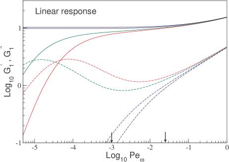
Figure 3: (Theory) The linear response moduli $G_{1}^{\prime}$ (full lines) and $G_{1}^{\prime\prime}$ (broken lines) as a function of $Pe_{\omega}$ for two statepoints in the fluid $\epsilon=-0.001$ (red), $-0.0005$ (green) and two in the glass $\epsilon=0.0005$ (blue), $0.001$ (black). For fluid states the finite value of the structural relaxation timescale is reflected in the maximum in $G^{\prime\prime}$ and the consequent crossing of $G^{\prime}$ and $G^{\prime\prime}$ at low frequency. The results presented here omit solvent hydrodynamics which may become relevant at $Pe_{\omega}\approx 1$ (calculations were performed with $\eta_{\infty}=0$). These will be included in a simple approximate fashion when fitting the experimental data. The two arrows indicate the values $Pe_{\omega}=0.001$ and $0.025$ used to generate Figs.4 and 5, respectively.

VI.1.3 Nonlinear stress response

By numerical solution of the equation of motion (III.1) we obtain the non-time translational invariant density correlator $\Phi(t,t^{\prime})$ and, via Eqs.(1) and (16), the nonlinear stress response. The numerical algorithm requires the equation of motion to be discretized over the entire two-dimensional $(t,t^{\prime})$-plane. While considerations of both causality ($t>t^{\prime}$) and the periodicity of the correlator with respect to a translation in time ($\Phi(t+t_{0},t^{\prime}+t_{0})=\Phi(t,t^{\prime})$, where $t_{0}=\pi/\omega$) enable certain simplifications to be made, calculation of the correlator over many decades in time remains a computationally demanding task.

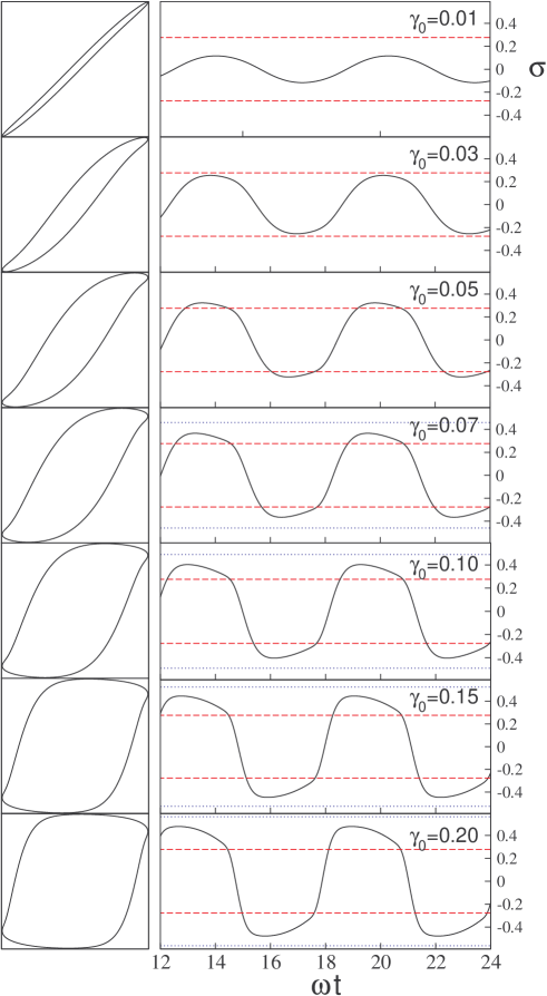
Figure 4: (Theory) The stress response of a glassy state to oscillatory strain calculated from our MCT based theory for strain amplitudes from $\gamma_{0}=0.01,0.03,0.05,0.07,0.10,0.15$ and $0.20$. The associated Lissajous figures illustrate the nonlinear character of the response. The increase in dissipation with increasing $\gamma_{0}$ is reflected by the increasing area enclosed by the Lissajous curves. All calculations were performed at $Pe_{\omega}=0.025$ and $\epsilon=0.001$. The red horizontal broken lines indicate the dynamic yield stress obtained from the flow curve in Figure.2 for $\epsilon=0.001$ ($\sigma_{y}=0.2763$). The response becomes clearly nonlinear when the maximum of $\sigma(t)$ approaches the dynamical yield stress. The blue horizonal dotted lines provide an upper bound for the maximum of the time-dependent stress and are taken from the corresponding flowcurve in Fig.2.

Typical examples of the response $\sigma(t)$ for a glassy state ($\epsilon=0.001$) are shown in Fig.4 for various values of the strain amplitude $\gamma_{0}$ at a fixed frequency. Alongside each of the time series we show the corresponding Lissajous curves indicating the extent of the dissipation (via the area enclosed, see Eq.(14)) and the deviations from nonlinearity (discernable from the non-ellipticity of the loop). The value of $\epsilon$ employed to generate this figure generates a dynamic yield stress $\sigma_{y}=0.2763$, which is indicated in each panel of Fig.4 by a broken red line. This can also be read-off from the appropriate flow curve in Fig.2.

For small amplitudes $\gamma_{0}\leq 0.01$ the system is almost linear and responds in a predominately elastic fashion at the considered frequency. As $\gamma_{0}$ is increased, clear deviations from a sinusoidal response are apparent and higher harmonics start to contribute to the signal. In this nonlinear regime the stress response exhibits a characteristically flattened peak, with an asymmetry which increases as a function of $\gamma_{0}$. It is clear from the figure that the higher harmonics first become significant when the maximum value of the stress $\sigma(t)$ approaches the dynamic yield stress. An idealized yield stress material, subject to large amplitude oscillatory shear of vanishing frequency, would be expected to show a steady increase of the stress up to the yield point, beyond which the system begins to flow, maintaining $\sigma(t)\!=\!\sigma_{y}$ until the reversal of strain enables relaxation back to zero. If this were the case, then $\sigma(t)$ would be represented by a ‘clipped’ signal, symmetric during loading and unloading of the sample.

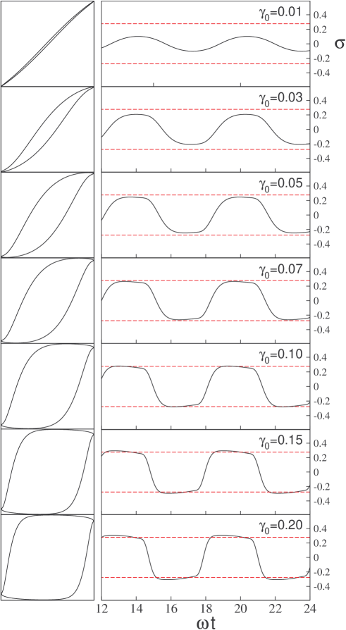
Figure 5: (Theory) As in Figure.3 ($\epsilon=0.001$) but for a lower frequency $Pe_{\omega}=0.001$. At this value of $Pe_{\omega}$ the system is almost perfectly elastic in the linear regime ($G^{\prime}\gg G^{\prime\prime}$ for $\gamma_{0}\ll 1$, see Figure.5). As the time-dependent stress exceeds the dynamical yield stress the signal becomes clipped. At this frequency $\sigma_{\rm max}$ lies very close to $\sigma_{y}$ and has thus been omitted for clarity.

The results presented in Fig.4, however, have been generated for a low, but not vanishingly small, frequency. At finite frequency the maximum stress attainable in a system under steady shear is given by $\sigma_{\rm max}\equiv\sigma(\gamma_{0}\omega)$, where $\sigma(\dot{\gamma})$ is the stress on the steady shear flow curve. This maximal stress under flow, $\sigma_{\rm max}$, is indicated by a blue dotted line in Fig.4, for the four largest strain amplitudes considered. In each case, once the stress exceeds the yield point the curve flattens, exhibiting a maximum which remains bounded from above by $\sigma_{\rm max}$. In the low frequency limit the lower and upper bounds to the peak value of $\sigma(t)$ become equal, $\sigma_{\rm max}\!=\!\sigma_{y}$, such that the signal becomes clipped at the yield point. In order to test this hypothesis further, we show in Fig.5 stress responses generated using the same parameter set as employed in Fig.4, but for a frequency one order of magnitude lower. At this reduced frequency, the clipping of $\sigma(t)$ at yield is quite clear, although the the peak stress still slightly exceeds $\sigma_{y}$, due to the fact that the values of the strain-rate amplitude are not sufficiently small that $\sigma_{\rm max}$ has saturated to $\sigma_{y}$.

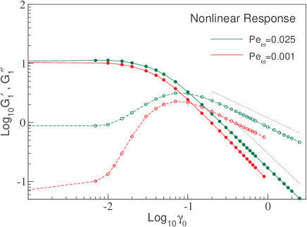
Figure 6: (Theory) The theoretical $G_{1}^{\prime}$ and $G_{1}^{\prime\prime}$ as a function of strain for $\epsilon=0.001$ at frequencies $Pe_{\omega}=0.025$ and $Pe_{\omega}=0.001$. Points are the numerically calculated data points, lines are a guide for the eye. For large values of the strain the numerical data are well fitted by the power laws $G^{\prime\prime}\sim\gamma_{0}^{-\nu}$ and $G^{\prime}\sim\gamma_{0}^{-2\nu}$ with $\nu=0.65$ (indicated by dotted lines).

Two additional comments are in order regarding the results shown in Figs.4 and 5. Firstly, for low frequencies (e.g. the data shown in Fig.5) the full time-dependent stress signal can be rather faithfully reproduced by the simple approximation

$$\sigma(t)=\begin{cases}\;\gamma_{0}[\,G_{1}^{\prime}(\omega)\sin(\omega t)+G_{1}^{\prime\prime}(\omega)\cos(\omega t)\,]\;\;\sigma\leq\sigma_{y}\\ \;\;0\hskip 147.38506pt\sigma>\sigma_{y}\end{cases}$$

where $G_{1}^{\prime}$ and $G_{1}^{\prime\prime}$ are the lowest order coefficients in the Fourier series (10). The naive picture sketched above is thus not completely correct. In order to describe correctly the sub-yield response, $\sigma(t)\leq\sigma_{y}$, it is neccessary to incorporate the $\gamma_{0}$ dependence of the lowest order coefficients; linear response is insufficient. It is also noteworthy that it is the dynamic, yield stress, which plays the crucial role in determining the time-dependent $\sigma(t)$. While the importance of dynamic yield in determining the oscillatory response is clear within the present approach, it remains to be seen whether this is a constraint introduced by employing a prescribed strain or, more significantly, an indication that the dynamic and static yield stresses are identical within our approximate theory. The simple approximation (VI.1.3) contains higher harmonic contributions as a result of the yield stress clipping criterion.

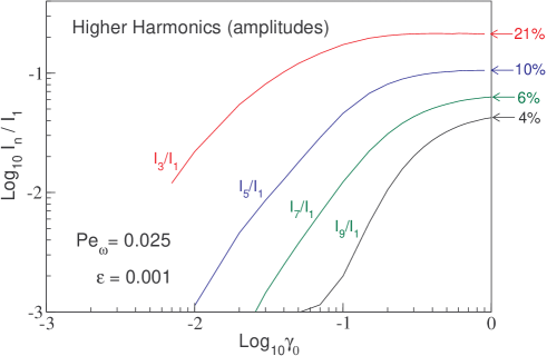
Figure 7: (Theory) The theoretical intensities of the third, fifth, seventh and ninth harmonic which contribute to the nonlinear stress response shown in Figure.3. At strains approaching unity the collective contribution of the higher harmonics accounts for approximately $50\%$ of the total $\sigma(t)$ signal. ($\epsilon=10^{-3}$ and $Pe_{\omega}=0.025$).

VI.1.4 Fourier analysis

In order to provide a more systematic analysis of the time signal $\sigma(t)$, we now consider its decomposition into Fourier modes and investigate the behaviour of the coefficients entering the series (10) and (13) as a function of $\gamma_{0}$. We address first the strain amplitude dependence of $G^{\prime}_{1}$ and $G^{\prime\prime}_{1}$, thus mimicing the ubiquitous ‘strain sweep’ experiments generally used to assess the nonlinear response of a given material. In Fig.6 we show typical results for the lowest order coefficients as a function of strain, for two different values of the excitation frequency.

For small values of $\gamma_{0}$ linear response is recovered and the values of $G^{\prime}_{1}$ and $G^{\prime\prime}_{1}$ may be read-off from the data shown in Fig.3. The linear response regime persists up to around $\gamma_{0}=0.01$, beyond which $G^{\prime\prime}_{1}$ begins to increase gradually, reaching a maximum value at around $\gamma_{0}=0.1$. As noted in subsection II.3, the coefficient $G^{\prime}_{1}$ is proportional to the amount of energy dissipated per oscillation cycle. The increase in dissipation observed over the range $\gamma_{0}=0.01\rightarrow 0.1$ is probably connected to the increasing disruption of the microscopic ‘cage’ structure of dense glassy systems, induced by the externally applied strain field. However, such microscopic interpretations remain purely speculative within the present context of schematic model calculations, for which there is no explicit spatial resolution of correlated density fluctuations.

Deeper insight into the microscopic mechanisms underlying the observed macroscopic response would be provided by solution of the full equations presented in joeprl_08 . The increase in $G^{\prime\prime}_{1}$ is associated with a decrease in $G^{\prime}_{1}$ as a function of $\gamma_{0}$. In contrast to $G^{\prime\prime}_{1}$, there exists no simple physical interpretation of the coefficient $G^{\prime}_{1}$ in the nonlinear regime. For strain amplitudes exceeding $\gamma_{0}=0.01$ the recoverable elastic energy becomes distributed over $G^{\prime}_{1}$ and the higher harmonics, such that $G^{\prime}_{1}$ loses its special status as a ‘storage modulus’.

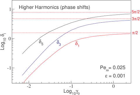
Figure 8: (Theory) The theoretical values for the first, third and fifth phase shift which contribute to the nonlinear stress response shown in Figure.3. It should be noted that the phases are only physically meaningful, i.e. contribute significantly to the total $\sigma(t)$ signal, when the corresponding intensities shown in Figure.7 are non-negligable. ($\epsilon=10^{-3}$ and $Pe_{\omega}=0.025$).

For $\gamma_{0}>0.1$ the dissipation $G^{\prime\prime}_{1}$ becomes larger than $G^{\prime}_{1}$, indicating a crossover from predominately elastic to predominately viscous response, and both functions exhibit a monotonic decay. For values of the strain amplitude larger than unity a regime of asymptotic decay is entered, characterized by a well defined power law dependence. We find that the numerically generated data are well fitted by power laws $G^{\prime\prime}_{1}\sim\gamma_{0}^{-\nu}$ and $G^{\prime}_{1}\sim\gamma_{0}^{-\nu^{\prime}}$, with $\nu=0.65(\pm 0.02)$ and $\nu^{\prime}=2\nu$. Moreover, calculations performed at various frequencies show that the exponent values are independent

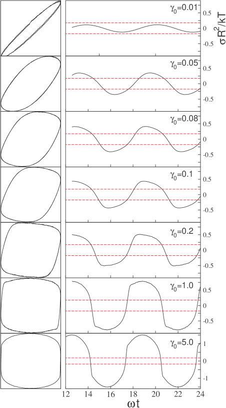
Figure 9: (Simulation) The stress response measured in Brownian dynamics simulations of a binary hard-disc mixture under oscillatory flow. A size ratio $1:1.4$ was used to supress crystallization. The considered strain amplitudes range from $\gamma_{0}=0.01$ to $\gamma_{0}=10$. The left column of figures shows the associated Lissajous curves illustrating the nonlinear character of the response. The simulations are performed at $\phi_{\rm tot}=0.81$ (slightly beyond the glass transition, according to our simulation estimates). The Peclet number is $Pe_{\omega}=0.05$).

of $\omega$ and thus seem to represent a universal aspect of the asymptotic decay within the schematic model. While the numerical findings are suggestive of a universal exponent $\nu$, analytical calulation of its precise value has so far proved elusive. The primary difficulty in extracting $\nu$ from the theory is that, even in the asymptotic regime, the correlator $\Phi(t,t^{\prime})$ retains a residual dependence upon the waiting time $t^{\prime}$ which does not yield readily to analytic treatment. The integral for the stress (1) thus consists of a complicated superposition of correlators for different values of $t^{\prime}$.

An important numerical prediction of the schematic model is that the exponents dictating the decay of $G^{\prime}$ and $G^{\prime\prime}$ are related, to within numerical accuracy, by a factor of $2$. The relation $\nu^{\prime}=2\nu$ has been observed in experimental studies of a variety of soft materials (see subsection VI.3 for more details on this point) and it would therefore be of considerable interest to investigate this apparent prediction of our model in more depth. The relationship $\nu^{\prime}=2\nu$ is found also in simple nonlinear Maxwell models faraday ; miyazaki3 , and is thus not particularly surprising. Such models inevitably predict the trivial exponents $\nu=1$ and $\nu^{\prime}=2$. The numerical data obtained by Miyazaki et al. miyazaki3 from solving their microscopic MCT theory is consistent with the exponent relation $\nu^{\prime}=2\nu$, but predicts a value of $\nu=0.9$ (obtained by fitting the numerical data), which differs somewhat from the experimental value $\nu=0.7$ for PMMA colloids presented in the same work. Whether the value $\nu=0.9$ from the MCT calculations of miyazaki3 is influenced by the additional isotropic approximations employed remains unclear.

The coefficients $G^{\prime}_{1}$ and $G^{\prime\prime}_{1}$ discussed above describe the response at the fundamental frequency. We now consider the contribution of the higher harmonic terms to the stress signal. Due to the $\dot{\gamma}(t)=-\dot{\gamma}(t)$ symmetry of $\sigma(t)$, even coefficients in the Fourier series (13) are identically zero within the schematic theory (a condition which provides a useful check for our numerical algorithms). In Fig.7 we show the intensities of the odd harmonics (normalized by $I_{1}$) up to $n=9$ for a glassy state, obtained by applying a discrete Fourier transform to the time series $\sigma(t)$. For very small amplitudes $\gamma_{0}<0.01$ the numerical solution of the equation of motion for $\Phi(t,t^{\prime})$ becomes unreliable, as the structural relaxation time exceeds the range of the numerical

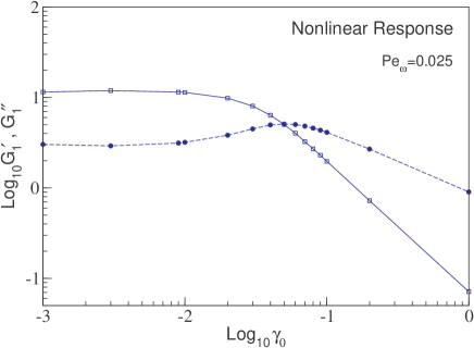
Figure 10: (Simulation) The simulation $G_{1}^{\prime}$ and $G_{1}^{\prime\prime}$ as a function of strain for two dimensional volume fraction $0.81$ and Peclet number $Pe_{\omega}=0.05$. For large values of $\gamma_{0}$ the moduli obey the power laws $G^{\prime\prime}_{1}\sim\gamma_{0}^{-0.68}$ and $G^{\prime}_{1}\sim\gamma_{0}^{-1.45}$.

grid upon which the oscillating function $\Phi(t,t^{\prime})$ can be resolved. Data are thus presented for $\gamma_{0}>0.01$ where accurate converged solutions can be obtained. At strain amplitude $\gamma_{0}=0.01$, only $I_{3}$ contributes significantly to the signal (around $3$%). As the $\gamma_{0}$ is increased beyond $0.01$, the increasing influence of $I_{3}$ is accompanied by the appearance of terms $I_{5}$, $I_{7}$ (beyond $\gamma_{0}=0.03$) and $I_{9}$ (beyond $\gamma_{0}=0.07$). Although intuitive, it is not clear a priori that the higher harmonics must neccessarily appear in sequence $n=3,5,7,\cdots$ upon increasing the amplitude. All of the $I_{n>3}$ exhibit a maximum in the range $0.3<\gamma_{0}<1$ and by $\gamma_{0}=1$ contribute approximately half of the total signal, $\sum_{n>1}I_{n}/I_{1}\sim 0.5$. The maximum and subsequent decay of the higher harmonics has also been observed in kallus .

Complementary to the higher harmonic intensities are the phase shifts $\delta_{n}$ shown in Fig.8. It should be noted that the phases are only physically meaningful for amplitudes at which the corresponding intensity is significant. As $\gamma_{0}$ is increased towards unity the phases saturate to the asymptotic values $\delta_{1}=\pi/2,\delta_{3}=3\pi/2$ and $\delta_{5}=5\pi/2$. The higher harmonic contributions $I_{n}$ and $\delta_{n}$, which contribute for $\gamma_{0}>0.01$, describe the distortion of $\sigma(t)$ close to the yield stress (c.f. Figs.4 and 5).

VI.2 Simulation results

In Fig.9 we show the stress response measured in our Brownian dynamics simulations of a binary hard-disc mixture. As the strain amplitude is increased the simulated stress evolves from a linear to a nonlinear response for $\gamma_{0}>0.03$. Consistent with the theoretical results shown in Fig.4, the time dependent signal becomes distorted away from a pure sinusoid when the peak of $\sigma(t)$ encounters the dynamic yield stress. Although the Peclet number $Pe_{\omega}=0.05$ is close to that employed in the theoretical calculations used to generate Fig.4, the onset of the yield stress clipping effect, already manifest in Fig.4, is not clear in the form of $\sigma(t)$ shown in Fig.9. It would therefore seem likely that considerably smaller values of the Peclet number are required to observe this effect in our two-dimensional simulations. Nevertheless, the general form of the nonlinear stress is very similar, on a qualitative level, to that predicted by the schematic model in Fig.4. Both simulation and theory exhibit a flattened and asymmetric peak which is skewed to the left.

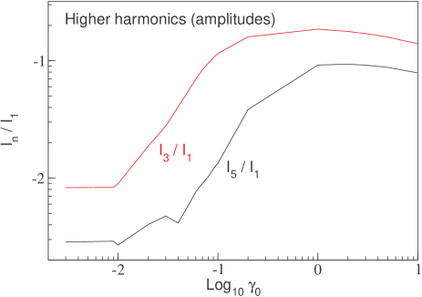
Figure 11: (Simulation) The normalized intensities of the third and fifth harmonic contributing to the nonlinear stress response shown in Figure.9.

In order to analyze more closely the stress signal we show in Figs.10, 11 and 12 the fundamental coefficients, higher harmonic intensities and phase shifts, respectively. The dependence of $G^{\prime}_{n}$ and $G^{\prime\prime}_{n}$ on $\gamma_{0}$ is strongly reminiscent of that predicted by the schematic model (Fig.6). Within the range $0.01<\gamma_{0}<0.06$ the system begins to deform plastically leading to a reduction in $G^{\prime}_{1}$ and an increase in $G^{\prime\prime}_{1}$ (and cross at $\gamma_{0}=0.05$), reflecting the increasing importance of dissipative processes. The height of the peak in $G^{\prime\prime}_{1}$ is rather less pronounced than that predicted by the schematic model. Beyond $\gamma_{0}=0.06$ both $G^{\prime}_{1}$ and $G^{\prime\prime}_{1}$ decrease monotonically, exhibiting an asymptotic power law decay which is well described by the power laws $G^{\prime\prime}_{1}\sim\gamma_{0}^{-0.68}$ and $G^{\prime}_{1}\sim\gamma_{0}^{-1.45}$. Although these values do not satisfy perfectly the empirical relation $\nu^{\prime}=2\nu$, the deviation of the simulation exponent ratio $\nu^{\prime}/\nu=2.13$ may well be attributable to numerical error. Despite this discrepancy, the absolute value of the exponents $\nu=0.68$ and $\nu^{\prime}=1.45$ compare well with those emerging from the schematic model ($\nu=0.65$ and $\nu^{\prime}=1.3$). The schematic model considered in the present work would thus seem to be more realistic than either a simple Maxwell model ($\nu=1$ and $\nu^{\prime}=2$) or the microscopic MCT approach of Miyazaki et al. ($\nu=0.9$ and $\nu^{\prime}=1.8$), at least on the basis of our simulation results.

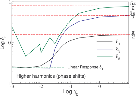
Figure 12: (Simulation) The phase shifts of the first and third harmonic contributing to the nonlinear stress response shown in Figure.9.

In Fig.11 we show the intensities of the third and fifth harmonic as a function of $\gamma_{0}$. Higher order terms were found to be highly susceptable to the effects of statistical noise in the simulation data and have thus been omitted. Upon increasing the strain amplitude beyond $\gamma_{0}=0.03$ the system leaves the linear response regime and the contribution of the third harmonic grows. For strains exceeding around $0.1$ the fifth harmonic also begins to play a significant role in determining the stress response. In keeping with the schematic models predictions, both $I_{3}/I_{1}$ and $I_{5}/I_{1}$ exhibit a maximum, albeit more sharply peaked and shifted to slightly larger strain values approaching unity. The corresponding phase shifts also share the general features of the schematic model predictions, in particular, for large values of $\gamma_{0}$ we find that $\delta_{1}$,$\delta_{3}$ and $\delta_{5}$ saturate to $\pi/2$, $3\pi/2$ and $5\pi/2$, respectively. These results suggest that the series (13) reduces to

$$\sigma(t)=\gamma_{0}\sum_{n=1}^{\infty}I_{2n+1}(\omega)(-1)^{n}\cos((2n+1)\,\omega t),$$ (27)

for large values of $\gamma_{0}$.

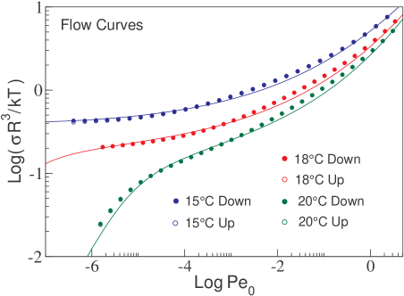
Figure 13: (Experiment) Symbols: The experimentally measured flowcurves for three different temperatures, $T=20$ ($\phi_{\rm eff}=0.57$), $T=18.4$ ($\phi_{\rm eff}=0.60$) and $T=15.1$ ($\phi_{\rm eff}=0.65$). Lines: Theoretical fits to the data using the parameters in table 1

VI.3 Experimental results

VI.3.1 Flow curves and linear response moduli

In Fig. 13 we show the experimentally measured flow curves and in Fig. 14 the linear response moduli for three different temperatures (corresponding to three different volume fractions). Reduced units are employed for both the control parameters

$$\mathit{Pe_{0}}=\frac{\dot{\gamma}R_{H}^{2}}{\mathit{D_{0}}},\hskip 28.45274pt\mathit{Pe_{\omega}}=\frac{\omega R_{H}^{2}}{\mathit{D_{0}}},$$

(where $D_{0}$ is obtained from the solvent viscosity using Stokes’ law) as well as for the shear stress and the moduli

$$\sigma_{\rm red}=\frac{\sigma R_{H}^{3}}{k_{B}T},\hskip 14.22636ptG^{\prime}_{\rm red}=\frac{G^{\prime}R_{H}^{3}}{k_{B}T},\hskip 14.22636ptG^{\prime\prime}_{\rm red}=\frac{G^{\prime\prime}R_{H}^{3}}{k_{B}T}.$$

For small Peclet numbers the flow curve measured at $20^{\circ}\,C$ (corresponding to $\phi_{\rm eff}=0.57$) shows a first Newtonian plateau. As $Pe_{0}$ is increased we observe a decrease in viscosity, followed by a second Newtonian plateau, both of which are typical for a shear thinning fluid. The viscoelastic character of the sample at $20^{\circ}\,C$ is demonstrated by the linear response moduli shown in Fig.14. For intermediate frequencies $G^{\prime}$ and $G^{\prime\prime}$ cross, indicating the presence of a structural $\alpha$-relaxation process.

The flow curve measured at the lower temperature $18^{\circ}\,C$ ($\phi_{\rm eff}=0.60$) displays a more pronounced plateau region. However, for the lowest frequencies investigated a slight decrease from the plateau is evident, suggesting the existence of an $\alpha$ relaxation time which has shifted out of the experimental frequency window. The corresponding linear moduli shown in Fig.14 show a distinctive plateau region of $G^{\prime}$ at intermediate values of $\mathit{Pe_{\omega}}$, followed by a decrease for small $\mathit{Pe_{\omega}}$ values, consistent with the existence of a crossover point and, therefore, a fluid relaxation. This is expecially apparent in $G^{\prime\prime}(\omega)$ which continues to rise as the frequency is decreased. Extrapolation of the measured data to lower frequencies suggests $\mathit{Pe^{\rm cross}_{\omega}}\approx 10^{-6}-10^{-7}$, where $G^{\prime}$ and $G^{\prime\prime}$ cross. For the lowest temperature investigated, 15${}^{\circ}\,C$ ($\phi_{\rm eff}=0.65$), the flow curve exhibits a constant plateau down to the lowest values of $Pe$ and the storage moduli remains constant at low $\mathit{Pe_{\omega}}$. The sample at 15${}^{\circ}\,C$ may thus be considered as a glass for which additional ‘hopping’ processes lead to an increase in $G^{\prime\prime}$ at low frequencies.

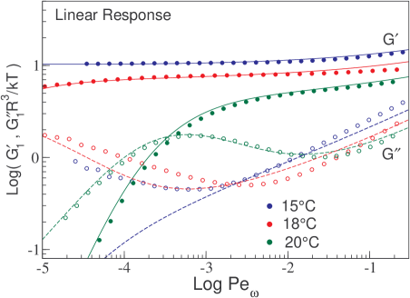
Figure 14: (Experiment) Symbols: The experimentally measured linear response moduli for three different temperatures, $T=20$ ($\phi_{\rm eff}=0.57$), $T=18.0$ ($\phi_{\rm eff}=0.60$) and $T=15.0$ ($\phi_{\rm eff}=0.65$). Lines: Theoretical fits to the data using the parameters in table 1

The procedure by which experimental data may be fit using the schematic F${}_{12}^{\dot{\gamma}}$ model of faraday is already well documented winter . Fitting the experimental data for the flow curve and linear moduli using the present schematic model proceeds analogously. For a given volume fraction, a fixed set of model parameters may be found which fit both the flow curve and the linear moduli. It is thus possible to determine the separation parameter $\epsilon$, the vertex $v_{\sigma}$ and the decay rate $\varGamma$. The parameter $\gamma_{c}$ is obtained as an additional parameter for the description of the flow curve. The high frequency viscosity $\eta_{\infty}^{\omega}$ is only important for the frequency spectrum (and is connected with the high shear viscosity $\eta_{\infty}^{\dot{\gamma}}$ via $\eta_{\infty}^{\dot{\gamma}}=\eta_{\infty}^{\omega}+v_{\sigma}/(2\varGamma)$ crassous ). Fixing the parameters by these two experiments in the linear viscoelastic and the steady state determines all information needed to calculate the nonlinear oscillatory behaviour (parameters are summarized in table 1). Therefore, the experimental data sets of the deformation sweeps (Figs. 15 - 17) and the oscillatory time tests (Figs. 18 and 19) are solely described by the theory of Section III and the fixed parameter sets obtained by fitting Figs. 14 and 13 without further modification. In this sense, the theoretical results to be presented for large amplitude oscillatory shear are predictions, as no further fitting is required.

Figure 15: (Experiment) Strain sweeps at three different frequencies for the temperature $15.0^{\circ}C$. Circles: Experimental data. Lines: Theoretical fits using the parameter set $(\epsilon,v_{\sigma},\Gamma,\gamma_{c},\tilde{x})$ obtained by simultaneously fitting the flow curves (Fig.13) and linear response moduli (Fig.14).

VI.3.2 Nonlinear response

The nonlinear regime has been tested using two different experiments: deformation sweeps at 1, 0.1 and 0.01 Hz (see Figs. 15 - 17) and oscillatory time series measured at 1, 0.1 and 0.01 Hz for various deformation amplitudes ranging from the linear to the non-linear regime (see Figs. 18 and 19). The complete set of nonlinear oscillatory data is solely described by the schematic MCT employing the parameter sets determined by the fitting procedure described above.

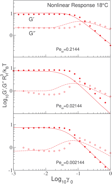
Figure 16: (Experiment) Strain sweeps at three different frequencies for the temperature $18.0^{\circ}C$. Circles: Experimental data. Lines: Theoretical predictions.

T [∘C]	$\phi_{\rm eff}$	$\epsilon$	$v_{\sigma}$	$\Gamma$	$\gamma_{c}$	$\eta_{\infty}$
20.0	0.57	$-2.45\times 10^{-3}$	59	100	0.18	42
18.0	0.60	$\;\;-2.2\times 10^{-4}$	85	100	0.19	36
15.0	0.65	$\;\;\;\;\;5\times 10^{-5}$	115	105	0.28	24

Table 1: Schematic model parameters obtained by fitting experimental data for the flow curves (Fig.13) and linear response moduli (Fig.14). These parameters are then used to make theoretical prediction for large strain amplitude oscillatory experiments.

In Fig.15 we show the results of strain sweep experiments at 15${}^{\circ}\,C$ ($\phi_{\rm eff}=0.65$) for three different values of $\mathit{Pe_{\omega}}$. For strains up to around 1% the system shows linear response behaviour, beyond which dissipation starts to increase, leading to a growth of $G^{\prime\prime}$ up to a maximum in the range 10-20% strain. The growing dissipation and eventual crossing of $G^{\prime}$ and $G^{\prime\prime}$ as a function of $\gamma_{0}$ indicate the breaking of microscopic particle cages.

For higher deformations $G^{\prime}$ and $G^{\prime\prime}$ display a power law decay. The exponents $\nu$ and $\nu^{\prime}$ obtained at different temperatures and frequencies are given in table 2

The theoretical predictions shown in Fig.15 are in excellent agreement with the experimental data and capture both the height and location of the maximum in $G^{\prime}$ rather well, although the departure from linear response appears to be less abrupt than in experiment, indicating a more gradual breaking of cages with increasing $\gamma_{0}$. We note that the discrepancy between theory and experiment in the linear response regime for the lowest frequency considered has its origins in the linear moduli fits presented in Fig.14. For glassy states there occur additional physical relaxation processes at low frequency which are manifest in an upturn of the linear response $G^{\prime\prime}(\omega)$ at low frequencies and which are not captured by mode-coupling based theoretical approaches. Particularly significant is the excellent agreement between theory and experiment in the large strain regime for which the cage structure has been broken up by the applied flow. The power law decay of the experimental data is well described by the theoretical exponents $\nu=0.65$ and $\nu^{\prime}=1.3$.

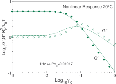
Figure 17: (Experiment) Strain sweeps at a fixed frequency $Pe_{\omega}=0.01917$ for the temperature $20^{\circ}C$. Circles: Experimental data. Lines: Theoretical predictions.

Both the numerically obtained theoretical results and experimental data shown here demonstrate the exponent relation $\nu^{\prime}\approx 2\nu$ (as in the theory of miyazaki3 ). It is interesting to note that although this relation does not appear to be truly universal, broadly similar behaviour has been found for a variety of different materials, all of which show the deformation behaviour classified by Hyun et al. Hyun02 as type III (weak strain overshoot). A few examples are e.g. a Xanthan gum solution McKinley10 with $\nu^{\prime}=-1.53$, $\nu=0.64$ and a ratio $\nu^{\prime}/\nu=2.4$, anchor spreadable butter and promise spread which yield exponents $-2.1<\nu^{\prime}<-2.0$ with $\nu=-0.9$ and a ratio of $\nu^{\prime}/\nu=2.3$, or the hard-sphere solution of Miyazaki et al. miyazaki3 (PMMA spheres of 197nm in a mixture of decaline and cycloheptylebromide) which show $\nu=0.7$ and $\nu^{\prime}=1.4$.

In Figs.16 and 17 we show further strain sweep measurements for temperatures 18${}^{\circ}\,C$ ($\phi_{\rm eff}=0.60$) and 20${}^{\circ}\,C$ ($\phi_{\rm eff}=0.57$). The overall level of agreement between theory and experiment is even better than that found for T=15${}^{\circ}\,C$. In particular, the strain sweep measured at 20${}^{\circ}\,C$ is very well described by the theory and, taken together with the results shown in Figs.13 and 14, demonstrate the accuracy with which the present schematic model may be used to describe the flow curve, linear moduli and strain sweep data of a dense colloidal fluid using a single fixed set of model parameters.

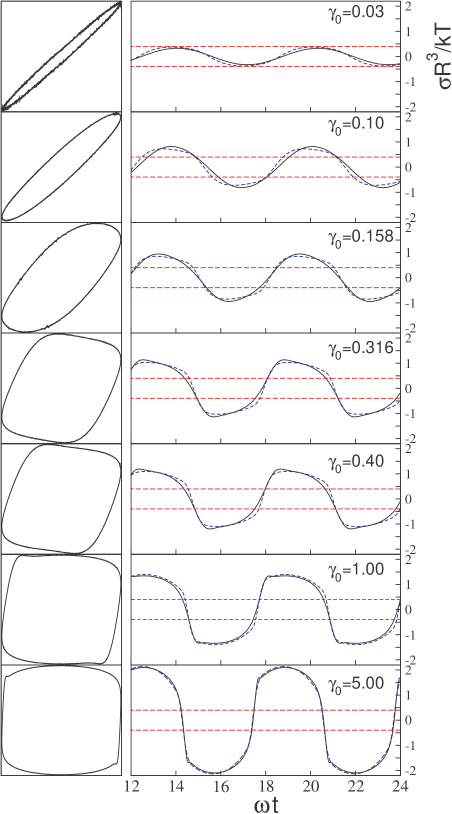
Figure 18: (Experiment) The stress response measured in LAOS experiments for strain amplitudes from $\gamma_{0}=0.03$ to $\gamma_{0}=5$ (black line) and the associated Lissajous figures illustrating the nonlinear character of the response. The experiments are performed at $T=15.1^{\circ}C$ a glassy state and at a frequency of $1Hz$ (corresponding to $\mathit{Pe_{\omega}}=0.02533$). At $\gamma_{0}=0.03$ the response is almost entirely elastic, emphasising the proximity of the quiescent state to the glass transition. At $\gamma_{0}=5$ the system is almost purely viscous. The increase in dissipation with increasing $\gamma_{0}$ is reflected in the increasing area enclosed by the closed Lissajous curves. The yield stress is indicated by the broken red lines. Theoretical results are given by broken blue lines.

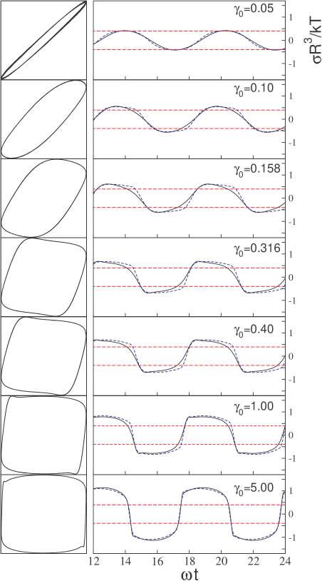
Figure 19: (Experiment) As in Fig.18 but at a frequency of $0.1Hz$ (corresponding to $Pe_{\omega}=0.002533$). Full black lines: Experimental data. Broken blue lines: Theoretical results. The yield stress is indicated by the broken red lines.

For the oscillatory time series the schematic model calculations and the simulation are in good agreement with the experimental data. The direct comparison of theory and experiment for two frequencies (1 Hz and 0.01 Hz) respectively the Peclet numbers ($\mathit{Pe_{\omega}}=0.025$ and 0.0025) is given in Figs. 18 and 19. For small deformations, a linear viscoelastic behaviour is indicated by the nearly perfect sinusoidal output signal, but becomes distorted as the strain amplitude is increased. For $\mathit{Pe_{\omega}}=0.025$ the stress signal displays flattened asymmetric peaks at intermediate values of $\gamma_{0}$, consistent with a regime of cage breaking around $\gamma_{0}=\gamma_{c}$. In contrast to the MCT predictions, the data show a pronounced dip at the top of the asymmetric peak. For high deformations, the peak shape approaches a semi-spherical shape with a vanishing but still visible dip or overshoot at the beginning edge of the peak. For the smaller frequency at $\mathit{Pe_{\omega}}=0.0025$ indications of the effect of the merging $\sigma_{max}$ and the yield stress are found. The peaks show in the intermediate and high deformation range a more cut off shape, although the dip still remains, in contradiction to the MCT. The peak shape for middle $\gamma_{0}$ drops faster in the experiment as for the more box-like shape of the MCT time signals. However this shape is found in the experiment for high $\gamma_{0}$ as well. Alltogether the experiments and the theory fit well for all compared Peclet numbers and amplitudes, although some small deviations of the shape exist. The predictive character of the schematic MCT model for the oscillatory time series is remarkable, due to the fact that the shapes are not fitted but calculated with the parameter set defined from the flow curves and the frequency test in the linear viscoelastic regime.

T [∘C]	$\phi_{\rm eff}$	$\omega$ [Hz]	$\nu$	$\nu^{\prime}$	$\nu^{\prime}/\nu$
15.0	0.65	1	-0.633	-1.262	1.99
15.0	0.65	0.1	-0.742	-1.404	1.89
15.0	0.65	0.01	-0.788	-1.555	1.97
18.0	0.60	1	-0.631	-1.297	2.06
18.0	0.60	0.1	-0.712	-1.424	2.00
18.0	0.60	0.01	-0.824	-1.630	1.98
20.0	0.57	1	-0.630	-1.250	1.98

Table 2: Experimentally measured values of the exponents $\nu$ and $\nu^{\prime}$ dictating the decay of $G^{\prime}$ and $G^{\prime\prime}$ as a function of $\gamma_{0}$ for large values of $\gamma_{0}$.

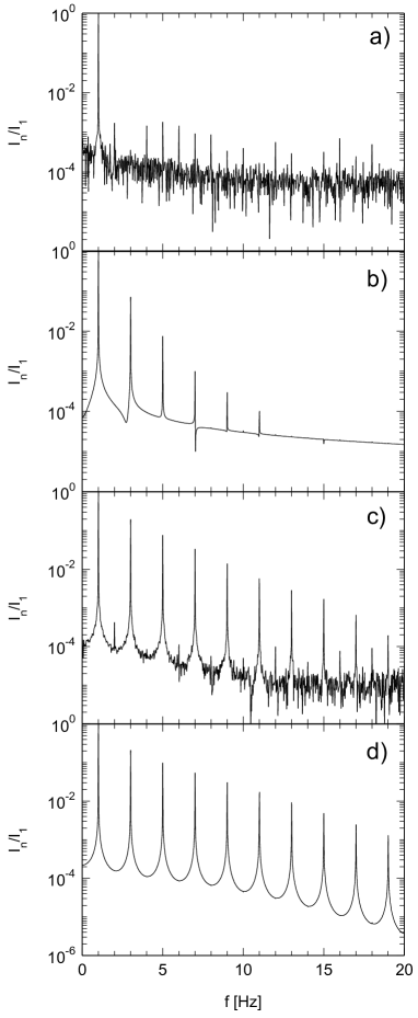
Figure 20: (Experiment and Theory) FFT-spectra of the oscillatory time test signals. The experiment was performed at 15.1${}^{\circ}\,$ and 1 Hz. $a)$ (experiment) and $b)$ (theory) are the FFT spectra at $\gamma_{0}=0.03$ and $c)$ (experiment) and $d)$ (theory) at an amplitude of $\gamma_{0}=1$.

VI.3.3 Fourier analysis

In order to provide a more detailed analysis of the time series shown in Figs.18 and 19 we have calculated the intensities and phase shifts (see Eq.(13)). The phase shifts are calculated from the real and imaginary parts of the Fourier transformed signal. Representative FFT-spectra are shown in Fig. 20 for the measurements made at at 15.1${}^{\circ}\,$C, 1 Hz and for amplitudes $\gamma_{0}=0.03$ and $1$. The spectrum demonstrates that at this low strain amplitude the higher harmonics do not contribute significantly and have an intensity only around 0.1% of the basic harmonic $I_{1}$. Although peaks for even and odd harmonics are visible, their low intensities are not far away from the noise level. We therefore consider this measurement to be within the linear viscoelastic range.

At the same conditions the MCT calculations show a rather different picture (see Fig. 20b). Although the time signals for this $\gamma_{0}$ do not deviate strongly from the experimental equivalent (see Fig. 20), the effect in the Fourier spectrum is noticable. Up to the 11th harmonic all odd harmonics can be clearly separated from the base line, with $I_{3}/I_{1}$ around 1%. Furthermore, in the theoretical FFT-spectrum an exponential decay of the intensities is apparent, a feature which first becomes evident in the exterimental data for $\gamma_{0}\geq 0.158$. At the larger strain amplitude, $\gamma_{0}=1$, the MCT calculations and the experimental FFT-spectra are very similar (see Fig. 20c and d). The present theory thus provides a qualitative description of the higher harmonics which becomes semi-quantitative as the strain amplitude becomes significant ($\gamma_{0}\sim 1$). The theory provides a sensible intperpolation between linear response and large amplitude regimes, both of which are captured accurately.

Some insight into the origin of the discrepancies at small excitation amplitude may be obtained by considering the theoretical predictions for the buildup of stress following the onset of steady shear flow (see also zausch ). Within the elastic regime (i.e. well below the ’stress overshoot’ identifying the yield strain) the system should display Hookian behaviour with a clearly defined elastic constant. However, schematic model calculations of the stress for this protocol (either using the present model or the $F_{12}^{\dot{\gamma}}$ model of faraday ) exhibit devaiations from Hookian behaviour at small strains. This feature of the schematic models is related to the slowness of the $\beta$ decay of the transient density correlator onto the plateau. We can thus speculate that the discrepancy between the Fourier spectra of theory and experiment at low values of $\gamma_{0}$ may be due to the excessively slow decay of the correlator to its plateau value, which is an inherent feature of any model based on the original schematic $F_{12}$ model MCTequations ; goetze_zeit ; sjoegren .

In Fig. 21a the amplitude dependence of the experimentally measured third harmonic is shown for three different frequencies in the glass (15.1${}^{\circ}\,$C). It can be seen that as the frequency is reduced, the onset of the nonlinear regime, indicated by increase of the normalized third harmonic intensity, moves to lower values of $\gamma_{0}$. In Fig. 21b we show the same quantity at a fixed frequency of 1Hz for three different temperatures. Surprisingly no strong influence of a change in the volume fraction is found, apart from a small deviation in the onset of the non-linear regime in the glassy state, which is shifted to higher deformations. The only significant deviation for the volume fractions considered occurs at intermediate deformations, as the starting and end values coincide.

The phase shifts are given for the measurement at 1 Hz ($\mathit{Pe_{\omega}}=0.025$) and 15${}^{\circ}\,$C in Fig. 21c. In the case of the fundamental $\delta_{1}$ the phase shift is found as expected to start at 0^∘ for small amplitudes and to end at 90^∘ for high deformations, which corresponds to a cosine. The curve progression of the experimental data and the MCT calculation fits perfectly for $\delta_{1}$. The theory deviates for the phase shifts of the higher harmonics due to the excessive contribution of non-linearities at lower $\gamma_{0}$. However, the limiting values for high deformations are found to coincide ($\frac{\pi}{2}$ for $\delta_{1}$, $\frac{3\pi}{2}$ for $\delta_{3}$ and $\frac{5\pi}{2}$ for $\delta_{5}$).

We have also included the data from our two-dimensional simulations into Figs. 21c and d. In order to obtain a reasonable comparison we found it neccessary to empirically multiply the strain employed in the simulations be a factor of three, $\gamma_{0}=3\cdot\gamma_{0}^{sim}$. That such an empirical rescaling is necessary is not surprising, given that only qualitative comparison is to be expected when comparing three dimensional experimental results with those of two dimensional simulations. It is therefore gratifying that the phases of the rescaled $\gamma_{0}^{sim}$ are found to describe the experimental data very well, not only for $\delta_{1}$ but also for $\delta_{3}$ and $\delta_{5}$.

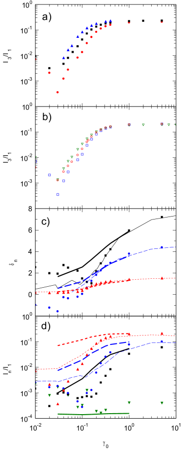
Figure 21: (Experiment and Theory) $a)$ $I_{3}/I_{1}$ at $15.1^{\circ}\,$C for different frequencies (red circle: 1 Hz, black square: 0.1 Hz and blue triangles up: 0.01 Hz). $b)$ Temperature dependence of $I_{3}/I_{1}$ at 1 Hz: $15.1^{\circ}\,$C (blue squares), 18.4${}^{\circ}\,$C (red circles) and 20.9${}^{\circ}\,$C (green triangles down). $c)$ Experimental phase shifts (symbols) for 15.1^∘C at 1 Hz. The simulation data is plotted versus $\gamma_{0}=3\gamma_{0}^{sim}$ as thin lines. The MCT calculations is given in thick lines. The phase shifts are $\delta_{1}$ (red triangles up and dotted lines), $\delta_{3}$ (blue circles and dashed lines) and $\delta_{5}$ (black squares and solid lines). $d)$ Normalized intensities at 15.1${}^{\circ}\,$C and 1 Hz; symbols mark the experimental data, thick lines the FFT of the MCT time signals and thin lines the shifted simulation results: $I_{2}/I_{1}$ (green triangles down and solid line), $I_{3}/I_{1}$ (red triangles up and dotted lines), $I_{5}/I_{1}$ (blue circles and dashed lines) and $I_{7}/I_{1}$ (black squares and solid line).

The experimentally measured $I_{3}/I_{1}$ at 15.1${}^{\circ}\,$C and 1 Hz is found to indicate the onset of the transition from linear to non-linear regime at around $\gamma_{0}=0.04-0.05$. This can be seen by comparing with the strain sweep data. It shows the maximum of $G^{\prime\prime}$ at $\gamma_{0}\approx 0.16$, which is connected with the breaking of the cages. This value could be correlated with the raising of $I_{5}/I_{1}$ above the ‘noise’ level of $0.1\cdot I_{1}/I_{1}$. The description of $I_{3}/I_{1}$ is possible with the formula obtained by Wilhelm ($I_{3/1}(\gamma_{0})=A\left[1-(1+(B\gamma_{0})^{c})^{-1}\right]$) wilhelm2 . For all experimental data the exponent $c$ or the slope of the increase is found to be in the range of $2.2-2.7$. The rescaled simulation results for the harmonics describe the experiment rather closely, whereas the MCT calcuations are found to show a different behaviour. All odd harmonics start at low $\gamma_{0}$ at higher values, whereas for high deformations the intensities coincide with the experimental results. Thus, also the slope of $I_{3}/I_{1}$ in this diagram changed to $c\approx 1.7$ instead of the experimental $c=2.7$. These discrepancies between experiment and theory may well be attributable to the slow decay of the correlator to the plateau, as discussed above.

Whereas the mode-coupling calcuations show a very early transition from the linear to the nonlinear regime at $\gamma\approx 0.01$ (see Figs. 15 to 17), for reasons discussed above, the experiments for the frequencies and temperatures investigated show a deviation from linear behaviour at $\gamma\approx 0.04-0.05$. For the rescaled simulation results of Fig. 10, the deviation starts at $\gamma\approx 0.03$. The onset of the yielding process is correlated with the onset of higher harmonics, starting with the third harmonic (see Fig. 21d). Although the difference of the onset and intensity of the higher harmonics between theory and experiment is significant, the time signals are only slightly influenced (Fig. 18 and 19). The FFT is a very sensitive method to analyse the time signals, so very small deviations in the time signal can cause a remarkable difference in the spectra. Increasing the strain amplitude results in more asymmetric time signals with maxima and minima shifted to the left.

It was found in experimental, theoretical and simulation strain sweeps that the maximum of $G_{1}^{\prime\prime}$ lies very close to the crossing point of $G_{1}^{\prime}(\gamma_{0})$ and $G_{1}^{\prime\prime}(\gamma_{0})$. For the glassy sample ($\phi=0.65$) this point was located at $\gamma\approx 0.15$. Beyond this value, the fifth harmonic begins to increase, which can be seen in Fig. 21d for the experimental and rescaled simulation data. The theoretical time signals do not show such a sharp transition from the linear to the nonlinear regime. Furthermore, the simulation data starts at higher intensity ratios as the experiment; an effect even more pronounced for the theoretical data. The schematic model thus predicts a more gradual transition between solid and fluid. The onset of the fifth harmonic was also found for micrometer sized particles Aksel02 to be correlated with the crossing point of $G_{1}^{\prime}$ and $G_{1}^{\prime\prime}$. The view that the yield strain is indicated by the onset of the fifth harmonic is supported by the results of Petekidis LeGrand08 . For larger deformations, the time signals show a strain softening behaviour, which is typical for shear thinning fluids. The phase shifts of experiment, simulation and theory approach the limiting values of $n\cdot\pi/2$, where $n$ is the index of the harmonic. In addition, the harmonics for theory and experiment show the same limiting values lat large $\gamma_{0}$ for each harmonic (21% for $I_{3}/I_{1}$, 10% for $I_{5}/I_{1}$, 6% for $I_{7}/I_{1}$ and 4% for $I_{9}/I_{1}$). Furthermore the theoretical harmonics exhibit a slight decrease at the highest calculated strains, which is not observed in the experimental data, perhaps due the choice of a too small measurment range. In the simulation the decrease of the intensities is much more pronounced for high deformations, as the intensities do not show a plateau but only a maximum (at 18% for $I_{3}/I_{1}$ and at 8% for $I_{5}/I_{1}$).

VII Conclusion and outlook

We have used a combination of theory, experiment and simulation to investigate the nonlinear stress response of dense colloidal dispersions under large amplitude oscillatory shear flow. The theory employed is a recent extension pnas of the well studied F${}_{12}^{\dot{\gamma}}$ model faraday . A key physical mechanism captured by the theory is the yielding of local particle cages and the subsequent onset of nonlinearity. In contrast to a related approach presented by Miyazaki et al. miyazaki1 ; miyazaki3 , the theory employed here makes predictions for the higher harmonic contributions to the stress signal and thus enables the extent of the linear response regime to be addressed. In order to make contact with experiment, the theory requires only the simultaneously determined parameters from the steady state flow curve and the frequency dependence of the linear moduli to make predictions for the nonlinear viscoelastic response. We have thus compared the theory with rheological experiments performed on concentrated suspensions of thermo-sensitive core-shell particles.

The first nonlinear experiment considered was a strain sweep, performed at three different volume fractions and frequencies. Here we found very good agreement between experiment and theory, although there are small deviations concerning the onset of the nonlinear viscoelastic regime. The values of $G_{1}^{\prime}$ and $G_{1}^{\prime\prime}$ in the linear regime, the crossing point of $G_{1}^{\prime}$ and $G_{1}^{\prime\prime}$, maximum of $G_{1}^{\prime\prime}$ and asymptotic large strain behaviour of $G_{1}^{\prime}$ and $G_{1}^{\prime\prime}$ are all well described by the theory. Brownian simulation of a two-dimensional system of hard discs enable only a qualitative comparison, but show behaviour broadly consistent with our experimental data, indicating that the yielding process is not strongly dependent upon either the material details or dimensionality of the sample. Moreover, the simulations do not contain hydrodynamic interactions, suggesting that these are not of great importance for yielding. The ratio of the slopes of $G_{1}^{\prime}$ and $G_{1}^{\prime\prime}$ for large $\gamma_{0}$ in the shear molten state yields the exponent ratio $\nu^{\prime}/\nu=2.0\pm 0.1$ in theory simulation and experiment. The fact that various other materials (of type III in Hyun02 ) display similar asymptotic behaviour may suggest a universal mechanism underlying the oscillatory response of shear molten viscoelastic fluids.

The second type of experiment considered were oscillatory time sweeps. In this case the cage yielding is expressed by the deviation of the signal from a sinusoidal form, showing a characteristic asymmetric peak in the yielding regime, which is followed in the shear molten state by a typical strain softening semi-circular peak shape. The agreement of the time signals obtained from theory, simulation and experiments is good. However, small deviations in the time series obtained using the three methods lead to stronger deviations in the parameters of the Fourier transformed time signals. This serves to emphasize the fact that FT-rheology is a very sensitive method, sensitive on the logarithmic scale, capable of detecting e.g. the fifth harmonic, to an accuracy of less than 1 promille. This analysis has shown that the onset of the third harmonic heralds the start of the nonlinear regime and that the maximum in $G_{1}^{\prime\prime}$, which here approximately coincides with the both crossing point of $G_{1}^{\prime}$ and $G_{1}^{\prime\prime}$ and the yield strain are correlated with the onset of the fifth harmonic. Moreover, the plateau values of the phase shifts at high deformations are found to follow $n\cdot\pi/2$ with $n$ beeing the index of each harmonic.

Despite the good overall level of agreement between theory and experiment there remain aspects which could be improved. Firstly, the extent (in $\gamma_{0}$) of the linear response regime is apparently too small within the present theory, with consequences for the variation of the higher harmonic intensities with amplitude. As noted, this failing has its origins in the quiescent transient density correlators predicted by the $F_{12}$ model, upon which our more recent schematic model is based. It would thus be desireable to improve this fundamental aspect of the theory. Secondly, the stress response measured in experiment displays a more asymmetric waveform than that predicted by the schematic model. This aspect can potentially be connected to the fact that our model, when applied to calculate the buildup of stress upon the onset of shear, does not generate a stress overshoot. While a stress overshoot does occur in approximate solutions of the fully microscopic mode-coupling expressions zausch , this aspect is lost in making the ansatz (16) for the shear modulus, as the strain dependent vertex functions appearing in the microscopic theory are replaced by a constant $v_{\sigma}$. Empirically reincorporating a strain dependence into the theory via the replacement $v_{\sigma}\rightarrow v_{\sigma}(\gamma_{0})$, such that the overshoot is recovered, may also lead to an increased waveform asymmetry in the stress response and, thus, better agreement with experiment. However, when modifying the schematic model in this fashion, care must be taken not to destroy its existing positive features.

To summarize, it can be concluded that the schmematic mode-coupling model pnas can make accurate predictions in the nonlinear viscoelastic regime, based purely on parameters fixed by the steady state stress and linear viscoelastic behaviour. This constitutes the first truly time-dependent test (other than step strain) of the schematic model proposed in pnas . Fourier transform analysis of time series obtained for various strain amplitudes and frequencies provides a wealth of experimental information regarding the mechanical response of a material. As our present experimental setup enables the investigation of transient flows, we anticipate that the study of such flow protocols, in combination with the present results, should enable a complete rheological characterization of our colloidal system.

Acknowledgements

Thanks to M. Schwall, J. Grzanna and A. Salah for helping with the programming of the FT-programm. Financial support was provided by the SFB TR6 and Swiss National Science Foundation (JMB) and the SFB 481 (MS).

References

- (1) R. G. Larson, The structure and rheology of complex fluids (Oxford, 1998).
- (2) P. Coussot, Rheometry of pastes, suspensions, and granualar materials (Wiley, 2005).
- (3) R.G. Larson, Constitutive equations for polymer melts and solutions (Butterworths, 1988).
- (4) M. Wilhelm, D. Maring and H-W. Spiess, Rheologica Acta 37 399 (1998).
- (5) M. Wilhelm, Macromol.Mater.Eng. 287 83 (2002).
- (6) R.H. Ewoldt, C. Clasen, A.E. Hosoi and G.H. McKinley, Soft Matter 3 634 (2007).
- (7) R.H. Ewoldt and P. Winter and J. Maxey and G. H. McKinley, Rheol. Acta 49 191 (2010).
- (8) R.H. Ewoldt, A.E. Hosoi and G.H. McKinley, J.Rheol. 52 1427 (2008).
- (9) F. Rouyer, S. Cohen-Addad, R. Höhler, P. Sollich and S.M. Fielding, Eur.Phys.J.E 27, 309 (2008).
- (10) C.O. Klein, H-W. Spiess, A. Calin, C. Balan and M.Wilhelm, Macromolecules 40 4250 (2007).
- (11) K.A. Cho, K. Hyun, K.H. Ahn and S.J. Lee, J. Rheol. 49 747 (2005).
- (12) M. Wilhelm, P. Reinheimer and M. Ortseifer, Rheol Acta 38 349 (1999).
- (13) S.A. Rogers and D. Vlassopoulos, J.Rheol. 54 859 (2010).
- (14) R. B. Bird, R.C. Armstrong and O. Hassager Dynamics of Polymeric Liquids (Wiley, 1987).
- (15) C. Truesdell and W. Noll, The Nonlinear Field Theories of Mechanics (Springer, Berlin, 1965).
- (16) P. Sollich, F. Lequeux, P. Hebraud and M.E. Cates, Phys.Rev.Lett. 78 2020 (1997).
- (17) S.M. Fielding, P. Sollich and M.E. Cates, J.Rheol. 44 323 (2000).
- (18) C. Derec, G. Ducouret, A. Ajdari, and F. Lequeux, Phys.Rev.E 67, 061403 (2003).
- (19) J.M. Brader, Th. Voigtmann, M.E. Cates and M. Fuchs, Phys.Rev.Lett. 98, 058301 (2007).
- (20) J.M. Brader, M.E. Cates and M. Fuchs, Phys.Rev.Lett. 101 138301 (2008), see also the associated Viewpoint article online in Physics 1, 22 (2008).
- (21) J. K. G. Dhont, An Introduction to the Dynamics of Colloids (Amsterdam, Elsevier, 1996).
- (22) M. Fuchs and M. E. Cates, Phys. Rev. Lett. 89, 248304 (2002).
- (23) M. Fuchs and M.E. Cates, J.Rheol. 53 957 (2009).
- (24) J.M. Brader, Th. Voigtmann, M. Fuchs, R.G. Larson and M.E. Cates, Proc. Natl. Acad. Sci. U.S.A. 106 15186 (2009).
- (25) J.M. Brader, J.Phys.:Condens.Matter 22 363101 (2010).
- (26) W. Götze, Liquids, Freezing and Glass Transition ed. J-P. Hansen, D. Levesque and J. Zinn-Justin (Amsterdam: North-Holland, 1991) p287.
- (27) M. Fuchs and M.E. Cates, Faraday Discussions 123, 267 (2003).
- (28) D. Hajnal and M. Fuchs, Eur.Phys.J.E 28, 125 (2009).
- (29) M. Fuchs and M. Ballauff, J.Chem.Phys. 122 094707 (2005).
- (30) J.J. Crassous et al, J.Chem.Phys. 125 204906 (2006).
- (31) J.J. Crassous, M. Siebenbürger, M. Ballauf, M. Drechsler, D. Hajnal, O. Henrich and M. Fuchs, J.Chem.Phys. 128 204902 (2008).
- (32) M. Siebenbürger, M. Fuchs, H. Winter and M. Ballauff, J.Rheol. 53 707 (2009).
- (33) W. Schärtl and H. Sillescu, J.Stat.Phys. 77 1007 (1994).
- (34) V. Carrier and G. Petekidis, J.Rheology 53 245 (2009).
- (35) J. Zausch, J. Horbach, M. Laurati, S.U. Egelhaaf, J.M. Brader, T. Voigtmann and M. Fuchs, J.Phys.:Condens.Matter 20 404210 (2008).
- (36) N.G. van Kampen, Chapter XV Section 3, in Stochastic Processes in Physics and Chemistry (North-Holland, Amsterdam, New York, Oxford 1981).
- (37) J.A. Lissajous, Ann.Chim.Phys. 51 147 (1857).
- (38) K. Miyazaki and D.R. Reichman, Phys.Rev.E 66 050501 (2002).
- (39) K. Miyazaki, D.R. Reichman and R. Yamamoto, Phys.Rev.E 70 011501 (2004).
- (40) K. Miyazaki, H.M. Wyss, D.A. Weitz and D.R. Reichmann, Europhys.Lett. 75 915 (2006).
- (41) See any standard text on Fourier series, e.g. M.L. Boas, Mathematical methods in the physical sciences (Wiley, 1983).
- (42) K. Hyun and M. Wilhelm, Macromolecules 42 411 (2009).
- (43) W. Götze, Z.Phys.B: Condens. Matter 56 139 (1984).
- (44) W. Götze and L.Sjögren, Rep.Prog.Phys. 55, 241 (1992).
- (45) H.M. Wyss et al, Phys.Rev.Lett. 98 238303 (2007).
- (46) M. Bayer, J.M. Brader, F.Ebert, M. Fuchs, E. Lange, G. Maret, R. Schilling, M. Sperl and J.P. Wittmer, Phys.Rev.E 76 011508 (2007).
- (47) N. Dingenouts, Ch. Norhausen and M. Ballauff, Macromolecules 31 8912 (1998).
- (48) K. Schmidt-Rohr and H.W. Spiess, Multidimensional solid state NMR and Polymers, (Academic Press, 1994).
- (49) D. van Dusschoten, M. Wilhelm, Rheol. Acta 40, 395 (2001).
- (50) D.A. Skoog and J.J. Leary, Principle of Instrumental Analysis, (Harcourt Brace College Publishers, Orlando, 4th edition, 1992).
- (51) C. Klein, Rheology and Fourier-Transform Rheology on water-based systems, Ph.D. thesis, Johannes-Gutenberg-Universität, Mainz, Germany (2005).
- (52) T. Neidhöfer, Fourier-transformation rheology on anionically synthesised polymer melts and solutions of various topology, Ph.D. thesis, Johannes-Gutenberg-Universit t, Mainz, Germany (2003).
- (53) S. Kallus, N. Willenbacher, S. Kirsch, D. Distler, T. Neidhöfer, M. Wilhelm and H.W. Spiess, Rheol.Acta 40 552 (2001).
- (54) R.N. Bracewell, The Fourier transform and its application, (McGraw-Hill 2nd edition, New York, 1986).
- (55) A. Scala, Th. Voigtmann and C. De Michele, J.Chem.Phys. 126 134109 (2007).
- (56) O. Henrich, F. Weysser, M.E. Cates and M. Fuchs, Phil. Trans. R. Soc. A 367, 5033 (2009).
- (57) G.G. Nair and S.K. Prasad and R. Bhargavi, V. Jayalakshmi and G. Shanker and C.V. Yelamaggad, J. Phys. Chem. B, 114, 697 (2010).
- (58) M.E. Helgeson and N.J. Wagner and D. Vlassopoulos, J. Rheol. 51, 297 (2007).
- (59) K. Hyun and S.H. Kim and K.H. Ahn and S.J. Lee, J. Non-Newtonian Fluid Mech. 107, 51 (2002).
- (60) K.N. Pham and G. Petekidis and D. Vlassopoulos and S.U. Egelhaaf and W.C.K. Poon and P.N. Pusey, J. Rheol. 52, 649 (2008).
- (61) L. Heymann and S. Peukert and N. Aksel, J. Rheol. 46, 93 (2002).
- (62) A. Le Grand and G. Petekidis, Rheol. Acta 47, 579 (2008).