DIAS-STP 10-11

Discrete Wilson Lines in F-Theory

Volker Braun

Dublin Institute for Advanced Studies¹
10 Burlington Road
Dublin 4, Ireland

Email: vbraun@stp.dias.ie

F-theory models are constructed where the $7$-brane has a non-trivial fundamental group. The base manifolds used are a toric Fano variety and a smooth toric threefold coming from a reflexive polyhedron. The discriminant locus of the elliptically fibered Calabi-Yau fourfold can be chosen such that one irreducible component it is not simply connected (namely, an Enriques surface) and supports a non-Abelian gauge theory.

1 Introduction

F-theory [1] is a way to use geometry as a tool to understand certain compactifications of string theory that are otherwise not entirely geometric [2]. It uses an auxiliary elliptically fibered Calabi-Yau fourfold, not to be confused with the space-time manifold to study string theory in a regime away from any known weakly-coupled perturbative description. Recently [3, 4] a particular model building Ansatz has been suggested where the GUT gauge group arises from a $7$-brane wrapped on a contractible del Pezzo surface. Various models [5, 6, 7, 8, 9, 10] and more have been constructed along these lines.

One key feature of this Ansatz is that the scales of gravity and gauge physics can be decoupled as one can decompactify the Calabi-Yau manifold without changing the del Pezzo surface. However, the price one has to pay for this is that the usual way of GUT symmetry breaking in string theory, namely the Hosotani mechanism[11, 12] using discrete Wilson lines, no longer works: All del Pezzo surfaces are simply connected. Alternatives have been developed [3, 4, 13], but require one to give a vacuum expectation value to fields locally and not just make global non-trivial identifications. Turning on fields locally then affects the running of the coupling constants and, potentially, defocus the gauge coupling unification [14, 15].

In this paper I will advocate for a different Ansatz for GUT model building and symmetry breaking in F-theory, namely, by wrapping the GUT $7$-brane on a non-simply connected divisor in the base of the elliptic fibration. This allows one to choose a globally non-trivial identification of the gauge bundle while keeping it locally trivial, breaking the GUT gauge group by the usual Hosotani mechanism. For what its worth, this setup also implies that there is no gravity/gauge theory decoupling limit.

Of course this raises the question of whether there are any such divisors in threefolds that are suitable as bases for elliptically fibered Calabi-Yau manifolds. In this paper I will answer this question and work out a rather simple example of an Enriques surface embedded into a toric threefold associated to a reflexive 3-dimensional polytope. There is nothing particularly unique about this example; It just combines the most simple surface with $\mathbb{Z}_{2}$ fundamental group and the class of threefolds we are most used to work with. All toric geometry computations used in this paper were done using [16, 17, 18].

2 Base Threefold

2.1 Foreword

An Enriques surface is a free quotient of a $K3$ surface by a freely-acting holomorphic involution and is probably the best-known example of a complex surface $S$ with fundamental group $\pi_{1}(S)=\mathbb{Z}_{2}$. Its first Chern class $c_{1}(S)$ is the torsion element in $H^{2}(Z,\mathbb{Z})\simeq\mathbb{Z}^{10}\oplus\mathbb{Z}_{2}$, so it admits a Ricci-flat metric but has no covariantly constant spinor. Some, but not all, $K3$ surfaces can be realized [19] as quartics in ${\mathop{\hbox{}{\mathbb{P}}}\nolimits}^{3}$. Somewhat unfortunately, the locus of quartic $K3$s and the locus of $K3$ surfaces with an Enriques involution do not intersect in the moduli space of smooth $K3$ surfaces. In other words, no smooth quartic in ${\mathop{\hbox{}{\mathbb{P}}}\nolimits}^{3}$ carries an Enriques involution. Therefore, out of necessity one is forced to look at singular (birational) models and then resolve these singularities. This will be the central theme in the following.

To explicitly construct and resolve the singularities, I will make extensive use of toric geometry. However, before delving into these technical details let me first give an overview. The basic idea is to look at the following $\mathbb{Z}_{4}$ action on ${\mathop{\hbox{}{\mathbb{P}}}\nolimits}^{3}$,

$$g:{\mathop{\hbox{}{\mathbb{P}}}\nolimits}^{3}\to{\mathop{\hbox{}{\mathbb{P}}}\nolimits}^{3},\quad\big{[}x_{0}:x_{1}:x_{2}:x_{3}\big{]}\big{[}x_{0}:ix_{1}:i^{2}x_{2}:i^{3}x_{3}\big{]}.$$ (1)

The fixed point set of $g^{2}$ are the two disjoint rational curves

$${\mathop{\hbox{}{\mathbb{P}}}\nolimits}^{1}\cup{\mathop{\hbox{}{\mathbb{P}}}\nolimits}^{1}=\big{\{}x_{0}=x_{2}=0\big{\}}\cup\big{\{}x_{1}=x_{2}=0\big{\}}$$ (2)

and the fixed points of $g$ are the north and south poles on these ($4$ points altogether). A sufficiently generic $\mathbb{Z}_{4}$ invariant quartic $q(x_{0},x_{1},x_{2},x_{3})$ is then a (singular) Enriques surface on the quotient. The fastest way to see this is to note that the would-be $(2,0)$-form

$$\Omega^{(2,0)}=\oint\frac{\epsilon^{ijk\ell}x_{i}\operatorname{d\!}x_{j}\wedge\operatorname{d\!}x_{k}\wedge\operatorname{d\!}x_{\ell}}{q(x_{0},x_{1},x_{2},x_{3})}$$ (3)

is projected out by $g$.

Here is where this paper essentially begins, because so far we only have a singular Enriques surface in an even more singular ambient space. Clearly, one wants to resolve the singularities. The first step is to resolve the curves of $\mathbb{Z}_{2}$ singularities, for which there is a unique crepant resolution. Then one has to deal with the remaining $4$ $\mathbb{Z}_{4}$ singularities. By a happy coincidence, the above $\mathbb{Z}_{4}$ quotient of ${\mathop{\hbox{}{\mathbb{P}}}\nolimits}^{3}$ is itself a toric variety. Hence, the methods of toric geometry can be applied and allow us to construct partial and complete resolutions explicitly as toric varieties.

2.2 Toric Geometry

As a warm-up, I will first review some basic notions of toric geometry. The defining data is a rational polyhedral fan in a lattice $N\simeq\mathbb{Z}^{d}$, where $d$ is the complex dimension of the variety. A fan $\Sigma$ is a finite set of cones $\sigma\in\Sigma$, closed under taking faces. Often, the fan will be the cones over the faces of a polytope. This is called the face fan of the polytope.

Amongst the different, but equivalent ways to define the corresponding complex algebraic variety from the fan data, I will use the Cox homogeneous coordinate [25] description in the following. The basic idea is to associate one complex-valued homogeneous coordinate to each ray (one-dimensional cone) of the fan. Then one has to remove a codimension-$2$ or higher algebraic subset and mod out generalized homogeneous rescalings. This construction will be reviewed and applied in much more detail in sec:cox. For now, let us just consider ${\mathop{\hbox{}{\mathbb{P}}}\nolimits}^{3}$ as an example. Its fan consists of the cones

$$\begin{split}\Sigma_{{\mathop{\hbox{}{\mathbb{P}}}\nolimits}^{3}}=\Big{\{}&\langle 0\rangle,\;\langle e_{1}\rangle,\;\langle e_{2}\rangle,\;\langle e_{3}\rangle,\;\langle-{\textstyle\sum}e_{i}\rangle,\;\\ &\langle e_{1},e_{2}\rangle,\;\langle e_{1},e_{3}\rangle,\;\langle e_{1},-{\textstyle\sum}e_{i}\rangle,\;\langle e_{2},e_{3}\rangle,\;\langle e_{2},-{\textstyle\sum}e_{i}\rangle,\;\langle e_{3},-{\textstyle\sum}e_{i}\rangle,\;\\ &\langle e_{1},e_{2},e_{3}\rangle,\;\langle e_{1},e_{2},-{\textstyle\sum}e_{i}\rangle,\;\langle e_{1},e_{3},-{\textstyle\sum}e_{i}\rangle,\;\langle e_{2},e_{3},-{\textstyle\sum}e_{i}\rangle,\;\Big{\}},\end{split}$$ (4)

where $e_{1}$, $e_{2}$, $e_{3}$ are a basis for $N\simeq\mathbb{Z}^{3}$. There are $4$ one-dimensional rays satisfying a unique linear relation, which translates into $4$ homogeneous coordinates with the usual identification

$$\big{[}x_{0}:x_{1}:x_{2}:x_{3}\big{]}=\big{[}\lambda x_{0}:\lambda x_{1}:\lambda x_{2}:\lambda x_{3}\big{]},\quad\lambda\in{\mathbb{C}}^{\times}.$$ (5)

A map of fans is a map of ambient lattices such that every cone of the domain maps into a cone of the range fan. Any such fan morphism defines a morphism of toric varieties in a covariantly functorial way. For the purposes of this paper, we will only consider the case where the lattice map is the identity. In this case the domain fan is simply a subdivision of the range fan. The toric map corresponding to a subdivision of a cone $\sigma$ is the blow-up along a toric subvariety of dimension equal to $\operatorname{codim}(\sigma)$.

A toric divisor is a formal linear combination $D=\sum a_{i}V(x_{i})$ of the codimension-one subvarieties

$$V(x_{i})=\big{\{}x_{i}=0\big{\}}$$ (6)

corresponding to the one-dimensional cones of the fan. There are two basic constructions associated to such a toric divisor that will be important in the following:

• Every coefficient $a_{i}$ can be thought of as the value of a function $f:N\to\mathbb{Z}$ on the generating lattice point $\rho_{i}$ of the $i$-th one-cone. If every cone is simplicial, then there is a uniquely defined continuous function on the fan with the above property. The pull-back of the function on the fan corresponds to the pull-back of the divisor by the toric map.

• The divisor also defines a polytope

  $$P_{D}=\big{\{}m\in M_{\mathbb{R}}\;\big{|}\;\langle m,\rho_{i}\rangle\geq-a_{i}\big{\}},$$ (7)

  where $M=N^{\vee}$ is the dual lattice. The global sections $\Gamma\mathscr{O}(D)$ are in one-to-one correspondence with the integral lattice points $M\cap P_{D}$ and can easily be counted for any given divisor.

A particularly relevant divisor is the anti-canonical divisor $-K=\sum V(x_{i})$. Given a polytope $\nabla\in N$, we can construct its face fan and the polytope $\Delta=P_{-K}\subset M$. If $\Delta$ is again a lattice polytope, then $\nabla$ is called reflexive.

Finally, note that $H^{2}({\mathop{\hbox{}{\mathbb{P}}}\nolimits}^{3})=\mathbb{Z}$. Hence, the line bundles on ${\mathop{\hbox{}{\mathbb{P}}}\nolimits}^{3}$ are classified by a single integer, their first Chern class. The toric divisors, on the other hand, are defined by $4$ integers. Clearly, there is no one-to-one correspondence between divisors $D$ and the isomorphism class of the associated line bundle $\mathscr{O}(D)$. To make this into a bijection, one must mod out linear equivalence of divisors. That is, one has to identify the piecewise linear functions modulo linear functions. In particular, one can easily see that

$$D=\sum_{i=0}^{3}a_{i}V(x_{i})~{}\sim~{}(a_{0}+a_{1}+a_{2}+a_{3})V(x_{0})$$ (8)

on ${\mathop{\hbox{}{\mathbb{P}}}\nolimits}^{3}$.

2.3 Three Birational Models

We now begin with the core of this paper and define the base threefold of the elliptically fibered Calabi-Yau fourfold. In fact, I will choose a smooth toric variety ${\hat{B}}$ as the base manifold, containing a non-simply connected divisor ${\hat{D}}$. However, directly analyzing ${\hat{B}}$ will be overly complicated. In particular, ${\hat{B}}$ contains exceptional divisors that do not intersect the divisor ${\hat{D}}$ we are interested in. Therefore, to better understand ${\hat{D}}\subset{\hat{B}}$, I will blow-down these additional exceptional divisors. This will produce a singular variety $B$ containing the same divisor $D={\hat{D}}$. Finally, I will blow-down two more curves in $B$ to obtain an (even more singular) three-dimensional variety ${\uline{B}}$. The blown-down divisor ${\uline{D}}\subset{\uline{B}}$ is the most suitable one to compute the fundamental groups. To summarize, I am going to define successive blow-ups

$${\hat{B}}\stackrel{{\scriptstyle\hat{\pi}}}{{\longrightarrow}}B\stackrel{{\scriptstyle\uline{\pi}}}{{\longrightarrow}}{\uline{B}}$$ (9)

of three-dimensional toric varieties. Both of the maps $\hat{\pi}$, $\uline{\pi}$ are toric morphisms defined in the obvious way by combining cones of the fan into bigger cones, discarding all rays that are no longer part of the more coarse (blown-down) fan.

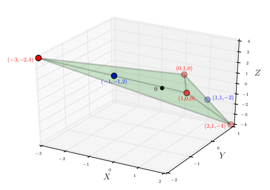
Figure 1: The rays $\Sigma^{(1)}_{\uline{B}}$ (red dots) and $\Sigma^{(1)}_{B}$ (red and blue dots).

I now define the fans $\Sigma$ corresponding to the toric varieties. Let me start by the rays $\Sigma^{(1)}$. The most singular variety has

$$\Sigma^{(1)}_{\uline{B}}=\big{\{}(-3,-2,4),\ (0,1,0),\ (1,0,0),\ (2,1,-4)\big{\}},$$ (10)

see fig:NablaBsing. The convex hull of these four points is a tetrahedron, but not a minimal lattice simplex. In addition to the origin (which is an interior point), it contains the two points $(-1,-1,2)$ and $(1,1,-2)$ along two different edges. The variety $B$ will be the maximal crepant partial resolution of ${\uline{B}}$, that is, the (in this case unique) maximal triangulation of the convex hull $\operatorname{conv}(\Sigma^{(1)}_{\uline{B}})$. Hence, one must add the additional integral points to the ray generators,

$$\Sigma^{(1)}_{B}=\Sigma^{(1)}_{\uline{B}}\cup\big{\{}(-1,-1,2),\ (1,1,-2)\big{\}},$$ (11)

Neither the variety ${\uline{B}}$ nor its maximal crepant partial resolution $B$ are smooth, related to the fact that the polytope $\operatorname{conv}(\Sigma^{(1)}_{\uline{B}})=\operatorname{conv}(\Sigma^{(1)}_{B})$ is not reflexive. One again needs to add rays to resolve all singularities, however this time the generators are necessarily outside of $\operatorname{conv}(\Sigma^{(1)}_{\uline{B}})$. One particular choice I am going to make are the rays generated by the $18$ points listed in tab:rays.

$i$	0	1	2	3	4	5	6	7	8	9	10	11	12	13	14	15	16	17
$i$-th ray	-3	0	1	2	-1	1	-2	-2	-1	-1	-1	0	0	1	1	1	2	2
	-2	1	0	1	-1	1	-1	-1	-1	0	0	0	0	0	0	1	1	1
	4	0	0	-4	2	-2	2	3	1	1	2	-1	1	-2	-1	-1	-3	-2
${\uline{B}}$	${\uline{z}}_{0}$	${\uline{z}}_{1}$	${\uline{z}}_{2}$	${\uline{z}}_{3}$
$B$	$z_{0}$	$z_{1}$	$z_{2}$	$z_{3}$	$z_{4}$	$z_{5}$
${\hat{B}}$	${\hat{z}}_{0}$	${\hat{z}}_{1}$	${\hat{z}}_{2}$	${\hat{z}}_{3}$	${\hat{z}}_{4}$	${\hat{z}}_{5}$	${\hat{z}}_{6}$	${\hat{z}}_{7}$	${\hat{z}}_{8}$	${\hat{z}}_{9}$	${\hat{z}}_{10}$	${\hat{z}}_{11}$	${\hat{z}}_{12}$	${\hat{z}}_{13}$	${\hat{z}}_{14}$	${\hat{z}}_{15}$	${\hat{z}}_{16}$	${\hat{z}}_{17}$

Table 1: Ray generators and the associated Cox homogeneous variables.

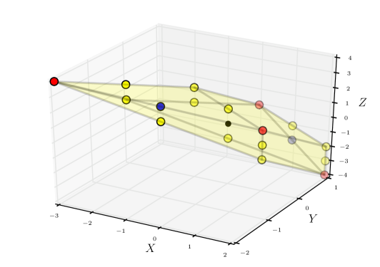
Figure 2: The rays $\Sigma^{(1)}_{\hat{B}}$.

The $8$ facets of the convex hull $\operatorname{conv}(\Sigma^{(1)}_{\hat{B}})$ are given by the inequalities

$$(n_{x},\,n_{y},\ n_{z})\cdot\left(\begin{array}[]{rrrrrrrr}-1&-1&-1&-1&0&1&1&2\\ -1&0&1&2&-1&-1&1&-1\\ -1&-1&0&0&0&0&1&1\end{array}\right)\geq(1,1,1,1,1,1,1,1),$$ (12)

which is, therefore, a reflexive polytope.

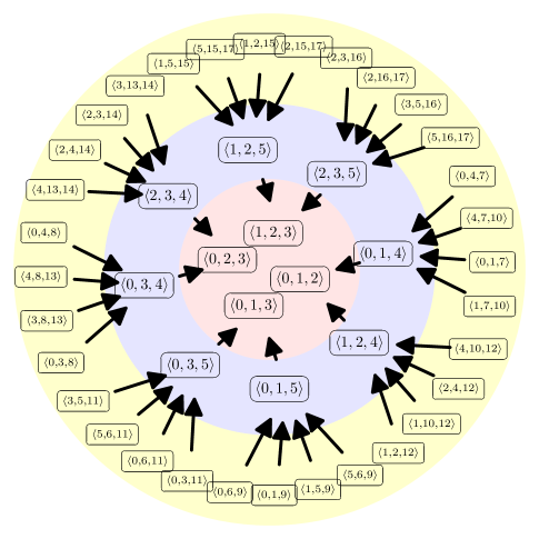
Figure 3: The generating cones of the fan $\Sigma_{\hat{B}}$ (yellow, outer circle), $\Sigma_{B}$ (blue), and $\Sigma_{\uline{B}}$ (red, inner circle). By $\langle i,j,k\rangle$ we denote the cone spanned by the rays number $i$, $j$, and $k$ in tab:rays, and arrows mean “contained in”.

Finally, to completely specify the toric varieties ${\uline{B}}$, $B$, and ${\hat{B}}$, let me define the generating cones of the respective fans:

• $\Sigma_{\uline{B}}$ is the face fan of the polytope $\operatorname{conv}(\Sigma^{(1)}_{\uline{B}})$, see fig:NablaBsing.

• $\Sigma_{B}$ is the unique maximal subdivision of $\Sigma_{\uline{B}}$.

• $\Sigma_{\hat{B}}$ is a maximal subdivision of the face fan of the polytope $\operatorname{conv}(\Sigma^{(1)}_{\hat{B}})$, see fig:NablaBsmooth.

As there are many different maximal subdivisions of the face fan, this alone does not uniquely specify the fan $\Sigma_{\hat{B}}$. For concreteness, I will fix the one listed in fig:fans_graph. Note that not all combinatorial symmetries of the graph in fig:fans_graph are actually symmetries of the fan.

2.4 Homogeneous Coordinates

For future reference, let me list the toric Chow groups [26]:

$$A_{k}({\hat{B}})=\begin{cases}1\\ \mathbb{Z}^{15}\\ \mathbb{Z}^{15}\\ 1\\ \end{cases},\quad A_{k}(B)=\begin{cases}1\\ \mathbb{Z}^{3}\times\mathbb{Z}_{2}\\ \mathbb{Z}^{3}\times\mathbb{Z}_{2}^{4}\\ 1\\ \end{cases},\quad A_{k}({\uline{B}})=\begin{cases}1&k=3\\ \mathbb{Z}\times\mathbb{Z}_{4}&k=2\\ \mathbb{Z}\times\mathbb{Z}_{2}^{2}&k=1\\ 1&k=0\\ \end{cases}$$ (13)

Since all three toric varieties have at most orbifold singularities, the Hodge numbers are $h^{p,p}=\operatorname{rank}A_{p}$ and $h^{p,q}=0$ if $p\not=q$.

The appearance of torsion in the Chow group slightly complicates the Cox homogeneous coordinate [25] construction of the toric varieties, so let me spell out the details. In general, a simplicial $d$-dimensional toric variety $X$ can be written as a geometric quotient

$$X=\frac{{\mathbb{C}}^{\Sigma^{(1)}_{X}}-Z}{\operatorname{Hom}\big{(}A_{d-1}(X),\;{\mathbb{C}}^{\times}\big{)}}\simeq\frac{{\mathbb{C}}^{r}-Z}{({\mathbb{C}}^{*})^{n-r}\times A_{d-1}(X)_{\text{tors}}},$$ (14)

where $r$ is the number of rays in the fan $\Sigma_{X}$. The exceptional set $Z$ is the variety defined by the irrelevant ideal. A more catchy way of remembering $Z$ is that it forbids homogeneous coordinates from vanishing simultaneously if and only if their product is a monomial in the Stanley-Reisner ideal. The latter is

$$\begin{split}SR(\Sigma_{\uline{B}})=&\;\big{<}{\uline{z}}_{0}{\uline{z}}_{1}{\uline{z}}_{2}{\uline{z}}_{3}\big{>},\\ SR(\Sigma_{B})=&\;\big{<}z_{0}z_{2},\ z_{1}z_{3},\ z_{4}z_{5}\big{>},\\ SR(\Sigma_{\hat{B}})=&\;\big{<}\cdots\text{105 quadric monomials}\cdots\big{>}.\end{split}$$ (15)

It remains to describe the groups in the denominator of eq. (14). For the most singular variety ${\uline{B}}$, one finds

$$\begin{split}\big{[}{\uline{z}}_{0}:{\uline{z}}_{1}:{\uline{z}}_{2}:{\uline{z}}_{3}\big{]}=&\;\big{[}\lambda{\uline{z}}_{0}:\lambda{\uline{z}}_{1}:\lambda{\uline{z}}_{2}:\lambda{\uline{z}}_{3}\big{]}\quad\forall\lambda\in{\mathbb{C}}^{\times},\\ \big{[}{\uline{z}}_{0}:{\uline{z}}_{1}:{\uline{z}}_{2}:{\uline{z}}_{3}\big{]}=&\;\big{[}{\uline{z}}_{0}:\mu{\uline{z}}_{1}:\mu^{2}{\uline{z}}_{2}:\mu^{3}{\uline{z}}_{3}\big{]}\quad\forall\mu\in\{1,i,i^{2},i^{3}\}\simeq\mathbb{Z}_{4}\end{split}$$ (16)

and for the intermediate blow-up $B$

$$\begin{split}\big{[}z_{0}:z_{1}:z_{2}:z_{3}:z_{4}:z_{5}\big{]}=&\;\big{[}\lambda z_{0}:\lambda z_{1}:\lambda z_{2}:\lambda z_{3}:z_{4}:z_{5}\big{]}\quad\forall\lambda\in{\mathbb{C}}^{\times},\\ \big{[}z_{0}:z_{1}:z_{2}:z_{3}:z_{4}:z_{5}\big{]}=&\;\big{[}\lambda z_{0}:z_{1}:\lambda z_{2}:z_{3}:\lambda^{-2}z_{4}:z_{5}\big{]}\quad\forall\lambda\in{\mathbb{C}}^{\times},\\ \big{[}z_{0}:z_{1}:z_{2}:z_{3}:z_{4}:z_{5}\big{]}=&\;\big{[}z_{0}:z_{1}:z_{2}:z_{3}:\lambda z_{4}:\lambda z_{5}\big{]}\quad\forall\lambda\in{\mathbb{C}}^{\times},\\ \big{[}z_{0}:z_{1}:z_{2}:z_{3}:z_{4}:z_{5}\big{]}=&\;\big{[}\mu z_{0}:\mu z_{1}:z_{2}:z_{3}:\mu z_{4}:z_{5}\big{]}\quad\forall\mu\in\{1,-1\}\simeq\mathbb{Z}_{2}.\end{split}$$ (17)

2.5 A Non-Simply Connnected Divisor

I am now going to define a divisor ${\uline{D}}\subset{\uline{B}}$ in the same linear system as the toric divisor

$${\uline{D}}\sim 4V({\uline{z}}_{0}),$$ (18)

that is, as the zero set of a sufficiently generic section of the line bundle $\mathscr{O}({\uline{D}})=\mathscr{O}\big{(}V({\uline{z}}_{0})\big{)}^{4}$. A basis for the sections is

$$H^{0}\big{(}{\uline{B}},\mathscr{O}({\uline{D}})\big{)}=\Big{<}{\uline{z}}_{0}^{4},\ {\uline{z}}_{2}^{4},\ {\uline{z}}_{1}^{4},\ {\uline{z}}_{3}^{4},\ {\uline{z}}_{1}{\uline{z}}_{2}^{2}{\uline{z}}_{3},\ {\uline{z}}_{1}^{2}{\uline{z}}_{3}^{2},\ {\uline{z}}_{0}{\uline{z}}_{2}{\uline{z}}_{3}^{2},\ {\uline{z}}_{0}{\uline{z}}_{1}^{2}{\uline{z}}_{2},\ {\uline{z}}_{0}^{2}{\uline{z}}_{2}^{2},\ {\uline{z}}_{0}^{2}{\uline{z}}_{1}{\uline{z}}_{3}\Big{>},$$ (19)

corresponding to the points of the polytope

$$P_{\uline{D}}=\operatorname{conv}\big{\{}(0,0,0),\ (4,0,2),\ (0,4,1),\ (0,0,-1)\big{\}}\subset M.$$ (20)

Note that the fan $\Sigma_{\uline{B}}$ is precisely the normal fan of the Newton polytope $P_{\uline{D}}$. In this sense, ${\uline{B}}$ is the “natural” ambient toric variety for the surface ${\uline{D}}$.

For explicitness, let me fix once and for all a linear combination of the monomials as the defining equation of the divisor ${\uline{D}}$. I will select the vertices of the Newton polytope and define

$${\uline{D}}=\Big{\{}{\uline{z}}_{0}^{4}+{\uline{z}}_{1}^{4}+{\uline{z}}_{2}^{4}+{\uline{z}}_{3}^{4}=0\Big{\}}\subset{\uline{B}}.$$ (21)

This surface is known to be an Enriques surface since it projects out the potential $(2,0)$-form as mentioned in sec:fore. In fact, this example has been known for some time, see Remark 3.6 in [27].

2.6 Kähler Cone and Canonical Divisors

The content of this subsection is not necessary for the understanding of the paper, but I would like to pause for a moment and mention how the “Fermat quartic” in eq. (21) fails to define a $K3$ surface. In other words, how does the divisor ${\uline{D}}=4V({\uline{z}}_{0})$ differ from the anticanonical divisor

$$-K_{\uline{B}}=V({\uline{z}}_{0})+V({\uline{z}}_{1})+V({\uline{z}}_{2})+V({\uline{z}}_{3})$$ (22)

of ${\uline{B}}$? Comparing with ${\mathop{\hbox{}{\mathbb{P}}}\nolimits}^{3}$, see eq. (8), one might have thought that they were linearly equivalent.

Similarly to the quartic $K3\subset{\mathop{\hbox{}{\mathbb{P}}}\nolimits}^{3}$, one can also define a Calabi-Yau variety in ${\uline{B}}$ as the zero locus of a section of the anticanonical bundle. The available sections are

$$H^{0}\big{(}{\uline{B}},\mathscr{O}(-K_{\uline{B}})\big{)}=\Big{<}{\uline{z}}_{0}^{2}{\uline{z}}_{3}^{2},\ {\uline{z}}_{0}^{3}{\uline{z}}_{2},\ {\uline{z}}_{2}^{2}{\uline{z}}_{3}^{2},\ {\uline{z}}_{0}{\uline{z}}_{2}^{3},\ {\uline{z}}_{1}{\uline{z}}_{3}^{3},\ {\uline{z}}_{0}{\uline{z}}_{1}{\uline{z}}_{2}{\uline{z}}_{3},\ {\uline{z}}_{0}^{2}{\uline{z}}_{1}^{2},\ {\uline{z}}_{1}^{2}{\uline{z}}_{2}^{2},\ {\uline{z}}_{1}^{3}{\uline{z}}_{3}\Big{>}.$$ (23)

Note that this differs from the sections of ${\uline{D}}$, see eq. (23). Therefore, the two divisor are not linearly equivalent. Nevertheless, $-K_{\uline{B}}$ and ${\uline{D}}$ are very close to being linearly equivalent. In fact, its easy to see that they are in the same rational divisor class since the rational divisor class group is one-dimensional, $\dim\big{(}A_{2}({\uline{B}})\otimes_{\mathbb{Z}}{\mathbb{R}}\big{)}=1$. However, their difference is a $2$-torsion element in the (integral) divisor class

$$K_{\uline{B}}+{\uline{D}}\not=0,\quad 2(K_{\uline{B}}+{\uline{D}})=0\quad\in A_{2}({\uline{B}})\simeq\mathbb{Z}\oplus\mathbb{Z}_{4}.$$ (24)

The same is true on the crepant partial resolution, where $K_{B}+D$ is again a 2-torsion element in $A_{2}(B)$.

On the final smooth resolution ${\hat{B}}$ the divisor class group $A_{2}({\hat{B}})=\mathbb{Z}^{15}$ is torsion free. However, the last blow-up $\hat{\pi}:{\hat{B}}\to B$ is not crepant, so

$$\hat{\pi}^{*}(K_{B})\not=K_{\hat{B}}.$$ (25)

Therefore, the divisors $-K_{\hat{B}}$ and ${\hat{D}}=\hat{\pi}^{*}(D)$ are no longer in the same rational equivalence class.

Finally, let me describe the Kähler cones of these varieties. First, let me remind the reader that the Kähler cone of a toric variety is an open rational polyhedral cone in the rational divisor class group corresponding to the cone of convex piecewise linear support functions on the fan. For the two singular varieties, one obtains

$$\mathcal{K}({\uline{B}})= \big{<}V({\uline{z}}_{0})\big{>} \subset ~{}A_{2}({\uline{B}})\otimes_{\mathbb{Z}}{\mathbb{R}}\simeq{\mathbb{R}}$$ (26)

$$\mathcal{K}(B)= \big{<}V(z_{0}),\ V(z_{1}),\ 2V(z_{0})+V(z_{4})\big{>} \subset ~{}A_{2}(B)\otimes_{\mathbb{Z}}{\mathbb{R}}\simeq{\mathbb{R}}^{3}$$

As the anticanonical class $-K_{\uline{B}}$ is rationally equivalent to $4V({\uline{z}}_{0})$, we see that

• ${\uline{B}}$ is a (singular) Fano variety.

• $B$ is not Fano, but the anticanonical class is on the boundary of the Kähler cone. In other words, $-K_{B}$ is nef but not ample.

On the smooth blow-up ${\hat{B}}$, the Kähler cone

$$\mathcal{K}({\hat{B}})\quad\subset~{}A_{2}({\hat{B}})\otimes_{\mathbb{Z}}{\mathbb{R}}\simeq{\mathbb{R}}^{15}$$ (27)

is rather complicated and we will refrain from listing it explicitly. It is spanned by the origin and $169$ rays and has $20$ facets. The anticanonical divisor $-K_{\hat{B}}$ as well as ${\hat{D}}$ sit on the boundary of the Kähler cone, that is, are nef but not ample. However, each satisfies a different subset of $16$ out of the $20$ facet equations, so they lie on different faces of the Kähler cone.

2.7 Pull-Back Divisors

By the usual dictionary of toric geometry, the toric divisor $4V({\uline{z}}_{0})\sim D$ corresponds to a continuous piecewise linear function on $N_{\mathbb{R}}\simeq{\mathbb{R}}^{3}$. Explicitly, the function is

$$f(n_{x},n_{y},n_{z})=\begin{cases}n_{z}&\text{if }\vec{n}\in\langle 0,1,2\rangle,\\ -4n_{x}-2n_{z}&\text{if }\vec{n}\in\langle 0,1,3\rangle,\\ -4n_{y}-n_{z}&\text{if }\vec{n}\in\langle 0,2,3\rangle,\\ 0&\text{if }\vec{n}\in\langle 1,2,3\rangle.\end{cases}$$ (28)

The pull-back of this toric divisor by the toric morphisms $\uline{\pi}$ and $\uline{\pi}\circ\hat{\pi}$ is simply given by the pull-back of the piecewise linear function. Therefore,

$$\begin{split}{\uline{D}}\sim&~{}4V({\uline{z}}_{0}),\\ D\sim&~{}4V(z_{0})+2V(z_{4}),\\ {\hat{D}}\sim&~{}4V({\hat{z}}_{0})+2V({\hat{z}}_{4})+4V({\hat{z}}_{6})+3V({\hat{z}}_{7})+3V({\hat{z}}_{8})+2V({\hat{z}}_{9})+\\ &~{}2V({\hat{z}}_{10})+2V({\hat{z}}_{11})+V({\hat{z}}_{12})+2V({\hat{z}}_{13})+V({\hat{z}}_{14}).\end{split}$$ (29)

What is the exceptional set of the first blow-up $\uline{\pi}$? Recall that it corresponds to the subdivisions along the 2-cones

$$\langle 0,4\rangle\cup\langle 2,4\rangle\to\langle 0,2\rangle,\quad\langle 1,5\rangle\cup\langle 3,5\rangle\to\langle 1,3\rangle,$$ (30)

see fig:NablaBsing. Therefore, $\uline{\pi}$ is the blow-up along two disjoint rational curves of $\mathbb{Z}_{2}$-singularities in ${\uline{B}}$. A standard intersection computation in the Chow group[26] yields that each curve intersects the divisor ${\uline{D}}$ in two points. Therefore, the proper transform of $D\subset B$ is ${\uline{D}}$ blown up in four points. The final blow-up $\hat{\pi}:{\hat{B}}\to B$ does not further subdivide the $2$-skeleton $\Sigma^{(2)}_{B}$ and, therefore, corresponds to the blow-up of points in $B$. Any sufficiently generic divisor $D$ misses these blow-up points and, therefore, the surfaces $D$ and ${\hat{D}}$ are isomorphic. To summarize,

• ${\uline{D}}$ is a singular Enriques surface with four $\mathbb{Z}_{2}$-orbifold points.

• ${\hat{D}}$ and $D$ are the same smooth Enriques surface after blowing up the orbifold points.

• Since the blow-up at a point does change the fundamental group, we find that

  $$\pi_{1}\big{(}{\uline{D}}\big{)}=\pi_{1}\big{(}D\big{)}=\pi_{1}\big{(}{\hat{D}}\big{)}=\mathbb{Z}_{2}.$$ (31)

It is important to remember that the actual divisor is a fixed subvariety defined as the zero locus of an equation. To relate this defining equation before and after the blow-up, it is instructional to write the first blow-up map $\uline{\pi}:B\to{\uline{B}}$ explicitly in terms of its action on homogeneous coordinates. One finds

$$\uline{\pi}\big{(}\big{[}z_{0}:z_{1}:z_{2}:z_{3}:z_{4}:z_{5}\big{]}\big{)}=\big{[}z_{0}\sqrt{z_{4}}:z_{1}\sqrt{z_{5}}:z_{2}\sqrt{z_{4}}:z_{3}\sqrt{z_{5}}\big{]}$$ (32)

Note that this map is well-defined on the equivalence classes eq. (17) thanks to the identifications eq. (16). One sees that, for example, the section ${\uline{z}}_{0}^{4}$ corresponds to the section $z_{0}^{4}z_{4}^{2}$ under the $\uline{\pi}^{*}$ pull-back. I leave the analogous expression for $\hat{\pi}$ as an exercise to the reader.

To summarize, the equation for the divisor ${\uline{D}}$ determines the equation satisfied by the proper transforms $D$ and ${\hat{D}}$ on the blow-ups. They are

$$\begin{split}{\uline{D}}=&\big{\{}{\uline{z}}_{0}^{4}+{\uline{z}}_{1}^{4}+{\uline{z}}_{2}^{4}+{\uline{z}}_{3}^{4}=0\big{\}},\\ D=&\big{\{}z_{0}^{4}z_{4}^{2}+z_{1}^{4}z_{5}^{2}+z_{2}^{4}z_{4}^{2}+z_{3}^{4}z_{5}^{2}=0\big{\}},\\ {\hat{D}}=&\big{\{}{\hat{z}}_{0}^{4}{\hat{z}}_{4}^{2}{\hat{z}}_{6}^{4}{\hat{z}}_{7}^{3}{\hat{z}}_{8}^{3}{\hat{z}}_{9}^{2}{\hat{z}}_{10}^{2}{\hat{z}}_{11}^{2}{\hat{z}}_{12}{\hat{z}}_{13}^{2}{\hat{z}}_{14}+{\hat{z}}_{1}^{4}{\hat{z}}_{5}^{2}{\hat{z}}_{6}^{2}{\hat{z}}_{7}^{2}{\hat{z}}_{9}^{3}{\hat{z}}_{10}^{4}{\hat{z}}_{11}{\hat{z}}_{12}^{2}{\hat{z}}_{15}^{3}{\hat{z}}_{16}{\hat{z}}_{17}^{2}+\\ &\phantom{\big{\{}}{\hat{z}}_{2}^{4}{\hat{z}}_{4}^{2}{\hat{z}}_{7}{\hat{z}}_{8}{\hat{z}}_{10}^{2}{\hat{z}}_{12}^{3}{\hat{z}}_{13}^{2}{\hat{z}}_{14}^{3}{\hat{z}}_{15}^{2}{\hat{z}}_{16}^{2}{\hat{z}}_{17}^{4}+{\hat{z}}_{3}^{4}{\hat{z}}_{5}^{2}{\hat{z}}_{6}^{2}{\hat{z}}_{8}^{2}{\hat{z}}_{9}{\hat{z}}_{11}^{3}{\hat{z}}_{13}^{4}{\hat{z}}_{14}^{2}{\hat{z}}_{15}{\hat{z}}_{16}^{3}{\hat{z}}_{17}^{2}=0\big{\}}.\end{split}$$ (33)

3 Elliptic Fibration

So far, I have constructed

• a three-dimensional (singular) Fano variety ${\uline{B}}$,

• a quasi-smooth divisor ${\uline{D}}$ in ${\uline{B}}$ with $\pi_{1}({\uline{D}})=\mathbb{Z}_{2}$,

• a smooth three-dimensional toric variety ${\hat{B}}$, corresponding to a maximal subdivision of a reflexive polytope, and

• a smooth divisor ${\hat{D}}$ in ${\hat{B}}$ with $\pi_{1}({\hat{D}})=\mathbb{Z}_{2}$. This divisor is a smooth Enriques surface.

I will now proceed and construct four-dimensional elliptically fibered Calabi-Yau varieties ${\uline{Y}}$, ${\hat{Y}}$ over ${\uline{B}}$ and ${\hat{B}}$ whose discriminant contains ${\uline{D}}$ and ${\hat{D}}$, respectively.

3.1 Weierstrass Models

Ideally, one would like to classify all elliptic fibrations over the base manifold. Unfortunately it is not known how to do so in this generality. It is known, however, that there exists a Weierstrass model (not necessarily over the same base) which is a (in general) different elliptic fibration [28, 29], at least assuming that the base is smooth and the discriminant is a normal crossing divisor. The Weierstrass model and the original elliptic fibration are birational to each other, but apart from that their relationship is arduous at best.

Having said this, let us define the elliptically fibered variety $Y$ in the most unimaginative way possible as a (global) Calabi-Yau Weierstrass model

$$Y=\Big{\{}y^{2}z=x^{3}+f(\vec{\zeta})xz^{2}+g(\vec{\zeta})z^{3}\Big{\}}~{}\subset~{}\mathbb{P}\Big{(}\mathscr{O}\oplus\mathscr{O}(-2K_{Z})\oplus\mathscr{O}(-3K_{Z})\Big{)},$$ (34)

on a base variety $Z$ with coordinates $\zeta$. The remaining coordinates, $z$, $x$, and $y$ are sections

$$z\in\Gamma\mathscr{O},\quad x\in\Gamma\mathscr{O}(-2K_{Z}),\quad y\in\Gamma\mathscr{O}(-3K_{Z}).$$ (35)

The defining data of the Weierstrass model is the choice of coefficients in the Weierstrass equation, that is, the choice of sections

$$f\in\Gamma\mathscr{O}(-4K_{Z}),\quad g\in\Gamma\mathscr{O}(-6K_{Z})$$ (36)

To engineer gauge theories on $7$-branes wrapped on a divisor $\{\zeta=0\}\subset Z$, one needs suitable singularities. In addition, the singularity must be of the correct split or non-split type as in Tate’s algorithm [30]. For this purpose it is convenient to parametrize the Weierstrass model by polynomials (that is, sections of suitable line bundles) $a_{1}$, $a_{2}$, $a_{3}$, $a_{4}$, $a_{6}$ as

$$\begin{split}f=&\;-\tfrac{1}{48}a_{1}^{4}-\tfrac{1}{6}a_{1}^{2}a_{2}+\tfrac{1}{2}a_{1}a_{3}-\tfrac{1}{3}a_{2}^{2}+a_{4}\\ g=&\;\tfrac{1}{864}a_{1}^{6}+\tfrac{1}{72}a_{1}^{4}a_{2}-\tfrac{1}{24}a_{1}^{3}a_{3}+\tfrac{1}{18}a_{1}^{2}a_{2}^{2}-\tfrac{1}{12}a_{1}^{2}a_{4}\\ &\;-\tfrac{1}{6}a_{1}a_{2}a_{3}+\tfrac{2}{27}a_{2}^{3}-\tfrac{1}{3}a_{2}a_{4}+\tfrac{1}{4}a_{3}^{2}+a_{6}.\end{split}$$ (37)

The degree of vanishing of the $a_{\ell}(\zeta)$ then determines the low-energy effective gauge theory, see [31, 32]. For everything to be globally defined, the $a_{\ell}$ need to be sections of

$$a_{\ell}\;\in\;\Gamma\mathscr{O}\big{(}-\ell K_{\hat{B}}\big{)}.$$ (38)

3.2 Weierstrass Model on the Singular Base

$\dim\Gamma\mathscr{O}(-\kappa K_{\uline{D}}-\delta{\uline{D}})$	$\kappa=1$	$\kappa=2$	$\kappa=3$	$\kappa=4$	$\kappa=5$	$\kappa=6$
$\delta=0$	$9$	$43$	$115$	$245$	$445$	$735$
$\delta=1$	$0$	$10$	$42$	$116$	$244$	$446$
$\delta=2$	$0$	$1$	$9$	$43$	$115$	$245$
$\delta=3$	$0$	$0$	$0$	$10$	$42$	$116$
$\delta=4$	$0$	$0$	$0$	$1$	$9$	$43$
$\delta=5$	$0$	$0$	$0$	$0$	$0$	$10$
$\delta=6$	$0$	$0$	$0$	$0$	$0$	$1$
$\delta\geq 7$	$0$	$0$	$0$	$0$	$0$	$0$

Table 2: Number of sections of $\mathscr{O}(-\kappa K_{\uline{D}}-\delta{\uline{D}})$.

To engineer a $SU(5)$ gauge theory coming from a $7$-brane wrapped on the divisor ${\uline{D}}$, one needs a split $A_{4}$ singularity [31]. This translates into $a_{\ell}$ vanishing to degree $\ell-1$ on ${\uline{D}}$. In other words, $a_{\ell}$ must be divisible by ${\uline{d}}^{\ell-1}=0$ where ${\uline{d}}$ is the defining equation for the divisor ${\uline{D}}$ as given in eq. (33). Put yet differently,

$$\frac{a_{\ell}}{{\uline{d}}^{\ell-1}}\;\in\;\Gamma\mathscr{O}\big{(}-kK_{\uline{D}}-(\ell-1){\uline{D}}\big{)}$$ (39)

The number of sections is tabulated in tab:DsingSections; Note how the rows repeat with periodicity $2$. This again follows from the fact that $K_{\uline{B}}$ and ${\uline{D}}$ differ by 2-torsion in the divisor class group, see eq. (24). Hence, there are plenty sections available for $a_{1}$, $\dots$, $a_{6}$ and one can easily find an elliptic fibration with a split $A_{4}$ over ${\uline{D}}$.

3.3 Weierstrass Model on the Smooth Base

Let me now turn to the smooth threefold ${\hat{B}}$ and construct a suitable singularity over the smooth divisor ${\hat{D}}$.

$\dim\Gamma\mathscr{O}(-\kappa K_{\hat{D}}-\delta{\hat{D}})$	$\kappa=1$	$\kappa=2$	$\kappa=3$	$\kappa=4$	$\kappa=5$	$\kappa=6$
$\delta=0$	$9$	$35$	$91$	$189$	$341$	$559$
$\delta=1$	$0$	$2$	$18$	$60$	$140$	$270$
$\delta=2$	$0$	$0$	$0$	$3$	$27$	$85$
$\delta=3$	$0$	$0$	$0$	$0$	$0$	$4$
$\delta\geq 4$	$0$	$0$	$0$	$0$	$0$	$0$

Table 3: Number of sections of $\mathscr{O}(-\kappa K_{\hat{D}}-\delta{\hat{D}})$, see also tab:DsingSections.

The main difference is that now, after resolving the singularity, the anticanonical divisor is “smaller” than ${\hat{D}}$, by which I mean that there are strictly less sections available for the Weierstrass model. See tab:DsmoothSections for details. Note that, if one always imposes the maximal degree of vanishing such that there are still non-zero sections, one can at most implement a split $A_{2}$ singularity leading to a low-energy $SU(3)$ gauge theory.

Having being dealt this lemon, let me try to make some lemonade. As in the previous subsection, I will write ${\hat{D}}=\{{\hat{d}}=0\}$ for the defining equation, see eq. (33). The split $A_{2}$ singularity corresponds to a factorized form

$$a_{1}= \;\alpha_{1} \qquad\alpha_{1}\in \;\Gamma\mathscr{O}(-K_{\hat{B}}),$$ (40)

$$a_{2}= \;{\hat{d}}\alpha_{2} \alpha_{2}\in \;\Gamma\mathscr{O}(-2K_{\hat{B}}-{\hat{D}}),$$

$$a_{3}= \;{\hat{d}}\alpha_{3} \alpha_{3}\in \;\Gamma\mathscr{O}(-3K_{\hat{B}}-{\hat{D}}),$$

$$a_{4}= \;{\hat{d}}^{2}\alpha_{4} \alpha_{4}\in \;\Gamma\mathscr{O}(-4K_{\hat{B}}-2{\hat{D}}),$$

$$a_{6}= \;{\hat{d}}^{3}\alpha_{6} \alpha_{6}\in \;\Gamma\mathscr{O}(-6K_{\hat{B}}-3{\hat{D}}).$$

A basis for all sections can, of course, be written as in terms of homogeneous monomials in the $18$ homogeneous coordinates ${\hat{z}}_{0}$, $\dots$, ${\hat{z}}_{17}$. To save a tree I will now switch to inhomogeneous coordinates $(\xi_{0},\xi_{1},\xi_{2})\in{\mathbb{C}}^{3}$ for the coordinate patch, say, corresponding to the cone $\langle 0,4,7\rangle$. This amounts to replacing the homogeneous coordinates with

$$\big{[}{\hat{z}}_{0}:{\hat{z}}_{1}:\cdots:{\hat{z}}_{17}\big{]}=\big{[}\xi_{0}:1:1:1:\xi_{1}:1:1:\xi_{2}:1:\cdots:1\big{]}$$ (41)

In this patch,

$${\hat{d}}=\xi_{0}^{4}\xi_{1}^{2}\xi_{2}^{3}+\xi_{1}^{2}\xi_{2}+\xi_{2}^{2}+1$$ (42)

and the sections of the relevant line bundles are

$$\begin{split}\Gamma\mathscr{O}(-K_{\hat{B}})=&\;\big{\langle}1,\xi_{1},\xi_{2},\xi_{0}\xi_{1}^{2}\xi_{2},\xi_{1}\xi_{2},\xi_{0}^{2}\xi_{1}\xi_{2},\xi_{0}^{2}\xi_{1}\xi_{2}^{2},\xi_{0}^{3}\xi_{1}^{2}\xi_{2}^{2},\xi_{0}\xi_{1}\xi_{2}\big{\rangle},\\ \Gamma\mathscr{O}(-2K_{\hat{B}}-{\hat{D}})=&\;\big{\langle}1,\xi_{0}^{2}\xi_{1}^{2}\xi_{2}\big{\rangle},\\ \Gamma\mathscr{O}(-3K_{\hat{B}}-{\hat{D}})=&\;\big{\langle}1,\xi_{1},\xi_{2},\xi_{1}\xi_{2},\xi_{0}^{2}\xi_{1}^{3}\xi_{2},\xi_{0}^{3}\xi_{1}^{4}\xi_{2}^{2},\xi_{0}^{2}\xi_{1}^{3}\xi_{2}^{2},\xi_{0}^{2}\xi_{1}\xi_{2},\xi_{0}^{2}\xi_{1}\xi_{2}^{2},\xi_{0}^{4}\xi_{1}^{3}\xi_{2}^{2},\\ &\;\phantom{\big{\langle}}\xi_{0}^{4}\xi_{1}^{3}\xi_{2}^{3},\xi_{0}^{5}\xi_{1}^{4}\xi_{2}^{3},\xi_{0}\xi_{1}^{2}\xi_{2},\xi_{0}^{2}\xi_{1}^{2}\xi_{2}^{2},\xi_{0}^{3}\xi_{1}^{3}\xi_{2}^{2},\xi_{0}\xi_{1}\xi_{2},\xi_{0}^{2}\xi_{1}^{2}\xi_{2},\xi_{0}^{3}\xi_{1}^{2}\xi_{2}^{2}\big{\rangle},\\ \Gamma\mathscr{O}(-4K_{\hat{B}}-2{\hat{D}})=&\;\big{\langle}1,\xi_{0}^{4}\xi_{1}^{4}\xi_{2}^{2},\xi_{0}^{2}\xi_{1}^{2}\xi_{2}\big{\rangle},\\ \Gamma\mathscr{O}(-6K_{\hat{B}}-3{\hat{D}})=&\;\big{\langle}1,\xi_{0}^{6}\xi_{1}^{6}\xi_{2}^{3},\xi_{0}^{2}\xi_{1}^{2}\xi_{2},\xi_{0}^{4}\xi_{1}^{4}\xi_{2}^{2}\big{\rangle}.\end{split}$$ (43)

For simplicity I will choose $\alpha_{\ell}$ to be the sum of the monomials corresponding to the vertices of the Newton polyhedron, that is,

$$\begin{split}\alpha_{1}=&\;\xi_{0}^{3}\xi_{1}^{2}\xi_{2}^{2}+\xi_{0}^{2}\xi_{1}\xi_{2}^{2}+\xi_{0}^{2}\xi_{1}\xi_{2}+\xi_{0}\xi_{1}^{2}\xi_{2}+\xi_{1}\xi_{2}+\xi_{1}+\xi_{2}+1,\\ \alpha_{2}=&\;\xi_{0}^{2}\xi_{1}^{2}\xi_{2}+1,\\ \alpha_{3}=&\;\xi_{0}^{5}\xi_{1}^{4}\xi_{2}^{3}+\xi_{0}^{4}\xi_{1}^{3}\xi_{2}^{3}+\xi_{0}^{4}\xi_{1}^{3}\xi_{2}^{2}+\xi_{0}^{3}\xi_{1}^{4}\xi_{2}^{2}+\\ &\;\xi_{0}^{2}\xi_{1}^{3}\xi_{2}^{2}+\xi_{0}^{2}\xi_{1}^{3}\xi_{2}+\xi_{0}^{2}\xi_{1}\xi_{2}^{2}+\xi_{0}^{2}\xi_{1}\xi_{2}+\xi_{1}\xi_{2}+\xi_{1}+\xi_{2}+1,\\ \alpha_{4}=&\;\xi_{0}^{4}\xi_{1}^{4}\xi_{2}^{2}+1,\\ \alpha_{6}=&\;\xi_{0}^{6}\xi_{1}^{6}\xi_{2}^{3}+1.\end{split}$$ (44)

For all purposes in the following, this choice is generic. By construction, the discriminant then factorizes as

$$\Delta=4f^{3}+27g^{2}={\hat{d}}^{3}\;{\hat{r}},$$ (45)

where the remainder defines a new divisor ${\hat{R}}\mathrel{\lower 0.28453pt\hbox{$\stackrel{{\scriptstyle\lower 1.27786pt\hbox{\scriptsize def}}}{{=}}$}}\{{\hat{r}}=0\}\sim-12K_{\hat{B}}-3{\hat{D}}$. In particular, the homology class splits as

$$[\Delta]=3[{\hat{D}}]+[{\hat{R}}]$$ (46)

Using the explicit equations, one can check [18] that

• ${\hat{R}}$ is an irreducible divisor.

• Neither $f$ nor $g$ vanish at a generic point of ${\hat{R}}$. Hence it supports $I_{0}$ Kodaira fibers in the Weierstrass model.

• ${\hat{D}}$ is smooth.

• ${\hat{R}}$ is not smooth, for example $(\xi_{0},\xi_{1},\xi_{2})=(1,1,-1)$ is a singular point.

• The curve ${\hat{D}}\cap{\hat{R}}$ is not a complete intersection.

Let me further investigate the intersection curve ${\hat{D}}\cap{\hat{R}}$. One component (in the $\langle 0,4,7\rangle$ patch) is given by the surprisingly simple expression

$$c:{\mathbb{C}}\to{\hat{D}}\cap{\hat{R}},~{}t\mapsto(t,0,i).$$ (47)

Therefore, $(\xi_{1},\xi_{2})$ are good normal coordinates. Taylor expanding along the normal directions for a generic point $c(t)$, we see that ${\hat{D}}$ and ${\hat{R}}$ share the same tangent plane but do not osculate to any higher degree. Therefore, the degree of vanishing of the discriminant jumps from $5$ to $7$ along the intersection locus ${\hat{D}}\cap{\hat{R}}$, corresponding to worsening of the $A_{2}$ singularity to an $A_{4}$ singularity.

4 Conclusions

In this paper I have constructed F-theory models with, a priori, $SU(5)$ gauge theory on a singular Fano threefold and a $SU(3)$ gauge theory on the blown-up smooth threefold. In both cases the non-Abelian gauge theory comes from a $7$-brane wrapped on an Enriques surface, which has fundamental group $\mathbb{Z}_{2}$. Therefore, in both cases one can switch on a discrete Wilson line and break the gauge group below the compactification scale in the usual manner.

The fact that the only partially resolved base $B$ allows for a higher rank gauge group on the $7$-brane than its smooth blow-up is curious: One might be tempted to interpret the Kähler deformation as the usual Higgs mechanism, however the singular points are disjoint from the $7$-brane. In any case, there must be further physical degrees of freedom associated to the singularities in the base and it would be nice to have a more concise F-theory dictionary for them.

Appendix A Fibrations of the Base

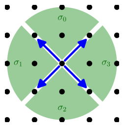
Figure 4: The fan defining the toric variety $S=\big{(}{\mathop{\hbox{}{\mathbb{P}}}\nolimits}^{1}\times{\mathop{\hbox{}{\mathbb{P}}}\nolimits}^{1}\big{)}/\mathbb{Z}_{2}$ (left) and its crepant smooth resolution ${\hat{S}}$ (right).

The base manifolds ${\uline{B}}$, $B$, and ${\hat{B}}$ are fibered in an interesting manner which I will describe in this appendix. The map to the $2$-dimensional base is given by the $N$-lattice projection

$$\phi:~{}N^{(3)}\to N^{(2)},\quad\vec{n}\mapsto\begin{pmatrix}1&1&1\\ -1&1&0\end{pmatrix}\vec{n}$$ (48)

This defines a toric morphism of toric varieties if and only if every cone of the domain fan is mapped into a cone of the range fan. It is easy to see that the rays $\Sigma^{(1)}_{\uline{B}}$ and $\Sigma^{(1)}_{B}$ map to the rays of the fan of $S=\big{(}{\mathop{\hbox{}{\mathbb{P}}}\nolimits}^{1}\times{\mathop{\hbox{}{\mathbb{P}}}\nolimits}^{1}\big{)}/\mathbb{Z}_{2}$, and the rays $\Sigma^{(1)}_{\hat{B}}$ map to the crepant resolution ${\hat{S}}$. See fig:SShat for a graphical representation of the fans of $S$ and ${\hat{S}}$.

However, consistently mapping the rays of the fans is not enough to define a toric morphism. Checking all higher-dimensional cones with respect to the lattice homomorphism $\phi$, one finds that

• The variety ${\uline{B}}$ is not fibered.

• The variety $B$ is a ${\mathop{\hbox{}{\mathbb{P}}}\nolimits}^{1}$-fibrations over $S$.

• The smooth threefold ${\hat{B}}$ is a ${\mathop{\hbox{}{\mathbb{P}}}\nolimits}^{1}$-fibration over $S$, but not over the crepant resolution ${\hat{S}}$.

It is, perhaps, vexing that the resolved threefold ${\hat{B}}$ is not a fibration over the resolved base ${\hat{S}}$. However, a closer investigation reveals that one can flop $4$ offending curves, corresponding to the $4$ bistellar flips

$$\begin{split}\big{\{}\langle 1,2,15\rangle,\langle 1,2,12\rangle\big{\}}\mapsto&\;\big{\{}\langle 1,12,15\rangle,\langle 2,12,15\rangle\big{\}}\\ \big{\{}\langle 0,1,9\rangle,\langle 0,1,7\rangle\big{\}}\mapsto&\;\big{\{}\langle 0,7,9\rangle,\langle 1,7,9\rangle\big{\}}\\ \big{\{}\langle 0,3,11\rangle,\langle 0,3,8\rangle\big{\}}\mapsto&\;\big{\{}\langle 0,8,11\rangle,\langle 3,8,11\rangle\big{\}}\\ \big{\{}\langle 2,3,16\rangle,\langle 2,3,14\rangle\big{\}}\mapsto&\;\big{\{}\langle 2,14,16\rangle,\langle 3,14,16\rangle\big{\}}\end{split}$$ (49)

of the fan $\Sigma_{\hat{B}}$. The flopped threefold is then a ${\mathop{\hbox{}{\mathbb{P}}}\nolimits}^{1}$ fibration over the resolved base ${\hat{S}}$. Of course the flopped threefold is then only birational to $B$, ${\uline{B}}$ and no longer a direct blow-up. However, it supports essentially the same elliptic fibration as ${\hat{B}}$ as constructed in sec:fibration.

Bibliography

• [1] C. Vafa, “Evidence for F-Theory,” Nucl. Phys. B469 (1996) 403–418, hep-th/9602022.
• [2] A. Sen, “F-theory and Orientifolds,” Nucl. Phys. B475 (1996) 562–578, hep-th/9605150.
• [3] C. Beasley, J. J. Heckman, and C. Vafa, “GUTs and Exceptional Branes in F-theory - I,” JHEP 01 (2009) 058, 0802.3391.
• [4] C. Beasley, J. J. Heckman, and C. Vafa, “GUTs and Exceptional Branes in F-theory - II: Experimental Predictions,” JHEP 01 (2009) 059, 0806.0102.
• [5] R. Donagi and M. Wijnholt, “Model Building with F-Theory,” 0802.2969.
• [6] J. Marsano, N. Saulina, and S. Schafer-Nameki, “F-theory Compactifications for Supersymmetric GUTs,” JHEP 08 (2009) 030, 0904.3932.
• [7] R. Blumenhagen, T. W. Grimm, B. Jurke, and T. Weigand, “Global F-theory GUTs,” Nucl. Phys. B829 (2010) 325–369, 0908.1784.
• [8] C.-M. Chen, J. Knapp, M. Kreuzer, and C. Mayrhofer, “Global SO(10) F-theory GUTs,” 1005.5735.
• [9] C.-M. Chen and Y.-C. Chung, “Flipped SU(5) GUTs from E8 Singularity in F-theory,” 1005.5728.
• [10] R. Blumenhagen, “Basics of F-theory from the Type IIB Perspective,” Fortsch. Phys. 58 (2010) 820–826, 1002.2836.
• [11] Y. Hosotani, “Dynamical Mass Generation by Compact Extra Dimensions,” Phys. Lett. B126 (1983) 309.
• [12] Y. Hosotani, “Dynamics of Nonintegrable Phases and Gauge Symmetry Breaking,” Ann. Phys. 190 (1989) 233.
• [13] R. Blumenhagen, V. Braun, T. W. Grimm, and T. Weigand, “GUTs in Type IIB Orientifold Compactifications,” Nucl. Phys. B815 (2009) 1–94, 0811.2936.
• [14] R. Donagi and M. Wijnholt, “Breaking GUT Groups in F-Theory,” 0808.2223.
• [15] R. Blumenhagen, “Gauge Coupling Unification in F-Theory Grand Unified Theories,” Phys. Rev. Lett. 102 (2009) 071601, 0812.0248.
• [16] V. Braun and A. Novoseltsev, “Toric Geometry in the Sage CAS.” to appear.
• [17] W. Stein et al., Sage Mathematics Software (Version 4.5.3). The Sage Development Team, 2010. http://www.sagemath.org.
• [18] G.-M. Greuel, G. Pfister, and H. Schönemann, “Singular 3.0,” a computer algebra system for polynomial computations, Centre for Computer Algebra, University of Kaiserslautern, 2005. \urlhttp://www.singular.uni-kl.de.
• [19] W. Nahm and K. Wendland, “A hiker’s guide to K3: Aspects of N = (4,4) superconformal field theory with central charge c = 6,” Commun. Math. Phys. 216 (2001) 85–138, hep-th/9912067.
• [20] V. Batyrev and M. Kreuzer, “Integral cohomology and mirror symmetry for Calabi-Yau 3-folds,” in Mirror symmetry. V, vol. 38 of AMS/IP Stud. Adv. Math., pp. 255–270. Amer. Math. Soc., Providence, RI, 2006.
• [21] B. Nill, “Gorenstein toric Fano varieties,” Manuscripta Math. 116 (2005), no. 2, 183–210.
• [22] V. Braun, “On Free Quotients of Complete Intersection Calabi-Yau Manifolds,” 1003.3235.
• [23] V. Braun, P. Candelas, and R. Davies, “A Three-Generation Calabi-Yau Manifold with Small Hodge Numbers,” Fortsch. Phys. 58 (2010) 467–502, 0910.5464.
• [24] P. Candelas and A. Constantin, “Completing the Web of $Z_{3}$ - Quotients of Complete Intersection Calabi-Yau Manifolds,” 1010.1878.
• [25] D. A. Cox, “The homogeneous coordinate ring of a toric variety,” J. Algebraic Geom. 4 (1995), no. 1, 17–50.
• [26] W. Fulton, Introduction to toric varieties, vol. 131 of Annals of Mathematics Studies. Princeton University Press, Princeton, NJ, 1993. The William H. Roever Lectures in Geometry.
• [27] M. Oka, “Finiteness of fundamental group of compact convex integral polyhedra,” Kodai Math. J. 16 (1993), no. 2, 181–195.
• [28] N. Nakayama, “Local structure of an elliptic fibration,” in Higher dimensional birational geometry (Kyoto, 1997), vol. 35 of Adv. Stud. Pure Math., pp. 185–295. Math. Soc. Japan, Tokyo, 2002.
• [29] N. Nakayama, “Global structure of an elliptic fibration,” Publ. Res. Inst. Math. Sci. 38 (2002), no. 3, 451–649.
• [30] J. Tate, “Algorithm for determining the type of a singular fiber in an elliptic pencil,” in Modular functions of one variable, IV (Proc. Internat. Summer School, Univ. Antwerp, Antwerp, 1972), pp. 33–52. Lecture Notes in Math., Vol. 476. Springer, Berlin, 1975.
• [31] M. Bershadsky et al., “Geometric singularities and enhanced gauge symmetries,” Nucl. Phys. B481 (1996) 215–252, hep-th/9605200.
• [32] K.-S. Choi, “SU(3) x SU(2) x U(1) Vacua in F-Theory,” 1007.3843.