Phase diagram of self-assembled rigid rods on two-dimensional lattices: Theory and Monte Carlo simulations

Abstract

Monte Carlo simulations and finite-size scaling analysis have been carried out to study the critical behavior in a two-dimensional system of particles with two bonding sites that, by decreasing temperature or increasing density, polymerize reversibly into chains with discrete orientational degrees of freedom and, at the same time, undergo a continuous isotropic-nematic (IN) transition. A complete phase diagram was obtained as a function of temperature and density. The numerical results were compared with Mean Field (MF) and Real Space Renormalization Group (RSRG) analytical predictions about the IN transformation. While the RSRG approach supports the continuous nature of the transition, the MF solution predicts a first-order transition line and a tricritical point, at variance with the simulation results.

I Introduction

Molecular self-assembly is one of the basic mechanisms of life and matter, and thus, modeling and measurements of naturally occurring self-assembling systems has long been pursued in the biological and physical sciences Pelesko ; Krasnogor . Despite the large number of papers that are currently reported, many of the ideas that are crucial to the development of this area (molecular shape, interplay between enthalpy and entropy, nature of the forces that connect the particles in self-assembled molecular aggregates) are simply not yet under the control of investigators.

Self-assembly also poses a number of substantial technological challenges Nalwa ; Whitesides ; Jiang ; Anderson ; Gooding ; Glotzer ; Glotzer1 ; Love ; Zaccarelli ; Alberts ; Lyons . In fact, the biological systems use self-assembly to assemble macromolecules and structures. Imitating these strategies and creating novel molecules with the ability to self-assemble into supramolecular assemblies is an important technique in nanotechnology. There is then a need for understanding the basic principles governing this type of organization.

It is obvious that a complete analysis of the self-assembly phenomenon is a quite difficult subject because of the complexity of the involved microscopic mechanisms. For this reason, the understanding of simple models with increasing complexity might be a help and a guide to establish a general framework for the study of this kind of systems, and to stimulate the development of more sophisticated models which can be able to reproduce concrete experimental situations.

Computer simulations have shown that spherical particles interacting isotropically through repulsive interparticle interactions can spontaneously assemble into anisotropic structures Likos ; Mladek ; Malescio . The presence of an isotropic short ranged interparticle attraction coupled to a longer ranged repulsion can also yield anisotropic structures. However, most real components, from proteins to ions De Yoreo to the wide variety of recently synthesized nanoparticles Glotzer ; Glotzer1 , interact via anisotropic or “patchy” attractions. Simulation work Duff ; Rein ; Gee ; Doye ; Auer reveals assembly pathways of such components to be in general richer than those of their isotropic counterparts. Experimental realization of such systems is growing. An example of real patchy particles is presented in Ref. [Cho, ]. Such particles offer the possibility to be used as building blocks of specifically designed self-assembled structures Whitesides ; Glotzer ; Glotzer1 ; Zhang1 ; Zhang2 . Moreover, the implications of patchy colloids for proteins Doye , which are patchy by nature, could be significant.

In this line, we consider in this paper the general problem of particles with strongly anisotropic, highly directional interactions in which effectively attractive patches induce the reversible self-assembly of particles into chains, i.e., equilibrium polymerization Sciortino ; Tavares ; Tavares1 ; PRE4 ; Tavares2 ; Tavares3 ; JCP13 . Recently, several research groups reported on the assembly of colloidal particles in linear chains. Selectively functionalizing the ends of hydrophilic nanorods with hydrophobic polymers, Nie et al. reported the observation of rings, bundles, chains, and bundled chains Nie . In another experimental study carried out by Chang et al. Chang , gold nanorods were assembled into linear chains using a biomolecular recognition system. In a direct relation with the present work, Clair et al. Clair investigated the self-assembly of terephthalic acid (TPA) molecules on the Au(111) surface. Using scanning tunneling microscopy, the authors showed that the TPA molecules arrange in one-dimensional chains with a discrete number of orientations relative to the substrate.

It is well known that solutions of self-assembled chains exhibit a transition from a disordered isotropic phase to an ordered nematic phase as the concentration of particles increases. Experimental examples of equilibrium polymer systems that exhibit a isotropic-nematic (IN) phase transition include wormlike micelles Hoffmann and self-assembled protein fibers like $f$-actin Oda ; Viamontes . In this context, a recent paper was devoted to the study of a system of self-assembled rigid rods adsorbed on a two-dimensional lattice Tavares . In Ref. [Tavares, ], Tavares et al. studied a system composed of monomers with two attractive (sticky) poles that polymerize reversibly into polydisperse chains and, at the same time, undergo a isotropic-nematic (IN) continuous phase transition foot0 . So, the interplay between the self-assembly process and the nematic ordering is a distinctive characteristic of these systems. Using an approach in the spirit of the Zwanzig model Zwanzig , the authors found that nematic ordering enhances bonding. In addition, the average rod length was described quantitatively in both phases, while the location of the ordering transition, which was found to be continuous, was predicted semiquantitatively by the theory. With respect to the characteristics of the phase transition, it has recently been shown that, at intermediate density, the IN transition is in the $q=1$ Potts universality class PRE4 .

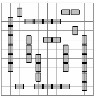
Figure 1: Schematic representation of a system of self-assembled rigid rods on a square lattice.

The temperature-coverage phase diagram obtained in Ref. [Tavares, ] is qualitative only, and the theory overestimates the critical temperature in all range of coverage. In addition, the possibility of a reentrant nematic transition at high densities Ghosh was not investigated by Tavares et al.. Accordingly, the main objective of the present work is to provide an accurate determination of the phase diagram of the system. For this purpose, extensive Monte Carlo (MC) simulations, supplemented by finite-size scaling analysis and two analytical approximations, have been carried out to obtain the critical temperature characterizing the IN phase as a function of the coverage. The paper is organized as follows. In Sec. II we describe the lattice-gas model. The simulation scheme and computational results are given in Sec. III. In Sec. IV we present the analytical approximations [Mean-Field approximation (MF), and Real Space Renormalization Group approach (RSRG)] and compare the MC results with the theoretical calculations. Finally, the general conclusions are drawn in Sec. V.

II Lattice-Gas Model

As in Refs. [Tavares, ; PRE4, ], we consider a system of self-assembled rods with a discrete number of orientations in two dimensions. We assume that the substrate is represented by a square lattice of $M=L\times L$ adsorption sites, with periodic boundary conditions. $N$ particles are adsorbed on the substrate with two possible orientations along the principal axis of the square lattice. These particles interact with nearest-neighbors (NN) through anisotropic attractive interactions (see Fig. 1). Then, the adsorbed phase is characterized by the Hamiltonian

$$H=-w\sum_{\langle i,j\rangle}|\vec{r}_{ij}\cdot\vec{\sigma}_{i}||\vec{r}_{ji}\cdot\vec{\sigma}_{j}|,$$ (1)

where $\langle i,j\rangle$ indicates a sum over NN sites; $w$ represents the NN lateral interaction between two neighboring $i$ and $j$, which are aligned with each other and with the intermolecular vector $\vec{r}_{ij}$; and $\vec{\sigma}_{i}$ is the occupation vector with $\vec{\sigma}_{i}=0$ if the site $i$ is empty, $\vec{\sigma}_{i}=\hat{x}$ if the site $i$ is occupied by a particle with orientation along the $x$-axis, and $\vec{\sigma}_{i}=\hat{y}$ if the site $i$ is occupied by a particle with orientation along the $y$-axis.

A cluster or uninterrupted sequence of bonded particles is a self-assembled rod. At fixed temperature, the average rod length increases as the density increases and the polydisperse rods will undergo an nematic ordering transition Tavares .

Since each site state is characterized by a three-state variable, we can rewrite Hamiltonian (1) in terms of new variables $S_{i}=0,\pm 1$, where where $S_{i}\pm 1$ represent the vertical ($\vec{\sigma}_{i}=\hat{y}$) and the horizontal ($\vec{\sigma}_{i}=\hat{x}$) orientations, while $S_{i}=0$ represents the empty state. Then, Hamiltonian (1) reads

$$H = -\frac{w}{4}\sum_{<i,j>}S_{i}S_{j}\left[(S_{i}+1)(S_{j}+1)(\hat{y}.\vec{r}_{ij})+(S_{i}-1)(S_{j}-1)(\hat{x}.\vec{r}_{ij})\right]$$ (2)

$$= -\frac{w}{4}\sum_{<i,j>}\left[(S_{i}^{2}+S_{i})(S_{j}^{2}+S_{j})(\hat{y}.\vec{r}_{ij})+(S_{i}^{2}-S_{i})(S_{j}^{2}-S_{j})(\hat{x}.\vec{r}_{ij})\right]$$

This Hamiltonian has the same energy spectrum as (1). Notice that the transformation $S_{i}\to-S_{i}$ is not a symmetry of the Hamiltonian (2), since it is equivalent to a $90^{o}$ rotation of the lattice, but it is a symmetry of the system, since it left the partition function unchanged. The total number of adsorbed particles can be written

$$N=\sum_{i}S_{i}^{2}$$ (3)

When $N=M$, we have $S_{i}^{2}=1$ and the Hamiltonian (2) results

$$H(\{S_{i}\})=-\frac{w}{4}\sum_{<i,j>}\left[1+S_{i}S_{j}+(S_{i}+S_{j})(\hat{y}.\vec{r}_{ij}-\hat{x}.\vec{r}_{ij})\right]$$ (4)

The last sum in Eq.(4) vanishes and therefore $H_{I}=-\frac{w}{4}\sum_{<i,j>}S_{i}S_{j}+$ constant. Hence, in that limit the present model reduces to the Ising one with coupling constant $w^{Ising}=w/4$.

III Monte Carlo Simulations

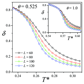
Figure 2: Size dependence of the order parameter as a function of temperature for $\theta=0.525$ and $\theta=1$ (inset).

III.1 Monte Carlo Method

We have used a standard importance sampling MC method in the canonical ensemble BINDER and finite-size scaling techniques PRIVMAN . The procedure is as follows. Starting with a random initial configuration (sites occupied with concentration $\theta=N/M$ and particle axis orientation chosen with probability $1/2$), successive configurations are generated by attempting to move single particles (monomers). One of the two (translation or rotation) moves is chosen at random. In a translation move, an occupied site and an empty site are randomly selected and their coordinates are established. Then, an attempt is made to interchange its occupancy state with probability given by the Metropolis rule Metropolis : $P=\min\left\{1,\exp\left(-\beta\Delta H\right)\right\}$, where $\Delta H$ is the difference between the Hamiltonians of the final and initial states and $\beta=1/k_{B}T$ (being $k_{B}$ the Boltzmann constant). For a rotation move, the rotational state of the chosen particle (horizontal or vertical) is changed with a probability determined by Metropolis criteria.

A Monte Carlo step (MCS) is achieved when $\theta\times M$ sites have been tested to change its occupancy state. Typically, the equilibrium state can be well reproduced after discarding the first $5\times 10^{6}$ MCS. Then, the next $6\times 10^{8}$ MCS are used to compute averages. All calculations were carried out using the parallel cluster BACO of Universidad Nacional de San Luis, Argentina. This facility consists of 60 PCs each with a 3.0 GHz Pentium-4 processor and 90 PCs each with a 2.4 GHz Intel Core 2 Quad processor.

In order to follow the formation of the nematic phase from the isotropic phase, we use the order parameter defined in Ref. [PRE4, ],

$$\delta=\frac{\left|N_{v}-N_{h}\right|}{N_{v}+N_{h}},$$ (5)

where $N_{h}(N_{v})$ is the number of monomers aligned along the horizontal (vertical) direction ($N=N_{h}+N_{v}$).

In our Monte Carlo simulations, we set the density $\theta$, varied the temperature $T$ and monitored the order parameter $\delta$, which can be calculated as simple averages. The reduced fourth-order cumulant, $U_{L}$, introduced by Binder BINDER , was calculated as:

$$U_{L}(T)=1-\frac{\langle\delta^{4}\rangle}{3\langle\delta^{2}\rangle^{2}},$$ (6)

where the thermal average $\langle...\rangle$, in all the quantities, means the time average throughout the MC simulation.

III.2 Computational results

The critical behavior of the present model has been investigated by means of the computational scheme described in the previous section and finite-size scaling analysis BINDER ; PRIVMAN .

We start with the calculation of the order parameter plotted versus the reduced temperature $T^{*}=k_{B}T/w$ for several lattice sizes ($L=60,80,100$ and $120$) and two values of coverage [$\theta=0.525$ foot1 , Fig. 2 and $\theta=1$, inset of Fig. 2]. As it can be observed, $\delta$ appears as a proper order parameter to elucidate the phase transition. When the system is disordered ($T^{*}>T^{*}_{c}$, being $T^{*}_{c}$ the critical temperature), all orientations are equivalents and $\delta$ is zero. In the critical regime ($T^{*}<T^{*}_{c}$), the particles align along one direction and $\delta$ is different from zero.

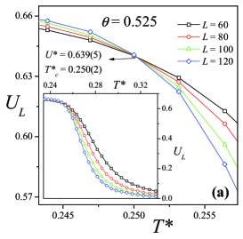
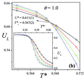
Figure 3: Curves of $U_{L}$ vs $T^{*}$ for $\theta=0.525$ (a) and $\theta=1$ (b). From their intersections one obtained $T^{*}_{c}$. In the insets, the data are plotted over a wider range of temperatures.

Hereafter we discuss the behavior of the critical temperature as a function of coverage. The standard theory of finite-size scaling allows for various efficient routes to estimate $T^{*}_{c}$ from MC data BINDER ; PRIVMAN . One of these methods, which will be used in this case, is from the temperature dependence of $U_{L}(T^{*})$, which is independent of the system size for $T^{*}=T^{*}_{c}$. In other words, $T^{*}_{c}$ can be found from the intersection of the curve $U_{L}(T^{*})$ for different values of $L$, since $U^{*}\equiv U_{L}(T^{*}_{c})=$const. As an example, Fig. 3 shows the reduced four-order cumulants $U_{L}$ plotted versus $T^{*}$ for the cases studied in Fig. 2. The values obtained for the critical temperature were $T^{*}_{c}=0.250(2)$ (corresponding to $\theta=0.525$) and $T^{*}_{c}=0.567(2)$ (corresponding to $\theta=1$). The procedure was repeated for $\theta$ ranging between $0$ and $1$. The results, which are collected in Fig. 4 (a), represent the temperature-coverage phase diagram of the system. The critical line (squares and line in the figure) separates regions of isotropic and nematic stability. The different phases are shown schematically in parts (b), (c) and (d) of Fig. 4.

With respect to the numerical results obtained by Tavares et al. at $\theta=0.2$ and $\theta=0.4$ [denoted with solid circles in Fig. 4 (a)], the agreement with the present data is very good.

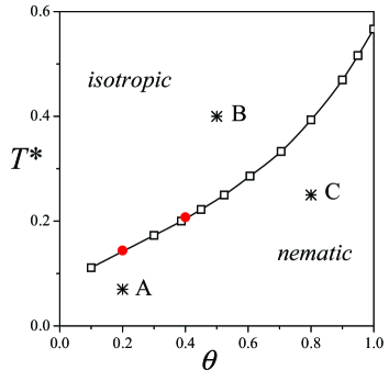
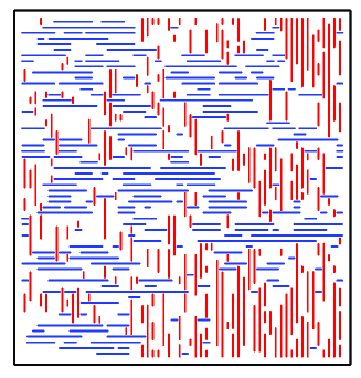
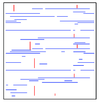
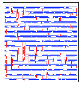
(a) (c) (b) (d)

Figure 4: (a) Phase diagram of the model: our simulation data (squares and line) and additional points (circles) obtained from Monte Carlo simulation, carried out by Tavares et al. Tavares . (b) Schematic representation of the low-density nematic phase (point A in the figure). (c) Same as (b) for the intermediate-density disordered phase (point B in the figure). (d) Same as (b) for the high-density nematic phase (point C in the figure).

As it is well-known, the behavior of the reduced fourth-order cumulant as a function of temperature not only provides an accurate estimation of the critical temperature $T_{c}$ in the infinite system, but also allows to make a preliminary identification of the order and universality class of the phase transition occurring in the system BINDER . In the case of Fig. 3, and as it is shown in the insets, the curves exhibit the typical behavior of the cumulants in the presence of a continuous phase transition. Namely, the order parameter cumulant shows a smooth drop from $2/3$ to $0$, instead of a characteristic deep (negative) minimum, as in a first-order phase transition BINDER .

With respect to the value of the intersection point $U^{*}$, two different behaviors can be visualized from Fig. 3. On one hand, at $\theta=0.525$, the value obtained for $U^{*}$ ($U^{*}=0.639(5)$) is consistent with the $q=1$ Potts universality class Wu observed in Ref. [PRE4, ], where the system was studied at a fixed temperature ($T^{*}=0.25$). On the other hand, and as it is expected for $\theta=1$, the fixed value of the cumulants, $U^{*}=0.611(1)$, is consistent with the extremely precise transfer matrix calculation of $U^{*}=0.6106901(5)$ for the 2D Ising model KAMIE . Even though the value of $U^{*}$ may be taken as a first indication of universality, a detailed calculation of critical exponents is required for an accurate determination of the universality class along the critical line in Fig. 4 (a), and this will be subject of future research.

Finally, Fig. 5 shows the nematic order parameter $\delta$ as a function of the coverage. The data correspond to $T^{*}=0.25$ and $L=100$ foot3 . As the density is increased above a critical value, the particles align along one direction and $\delta$ increases continuously to one, remaining constant up to full coverage. In other words, nematic order survives until $\theta=1$. This finding $(1)$ allows us to discard the existence of a reentrant nematic transition at high densities as speculated in Ref. [Tavares, ] and $(2)$ indicates a substantial difference between the present system and that of monodisperse rigid rods without self-assembly, where a second nematic to isotropic phase transition is observed at high densities Ghosh ; JSTAT1 .

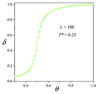
Figure 5: Nematic order parameter $\delta$ as a function of the coverage. The data correspond to $T^{*}=0.25$ and $L=100$.

IV Analytical Approximations and Comparison Between Simulated and Theoretical Results

In this section we calculate the phase diagram within mean field and real space renormalization group approaches. Let

$$f\equiv-\frac{1}{M\beta}\ln\left[{\rm Tr}\,e^{-\beta H^{\prime}}\right]$$ (7)

the grand canonical free energy, where $H^{\prime}=H-\mu N$, $H$ and $N$ are given by Eqs. (2) and (3), and $\mu$ is the chemical potential. The orientational order parameter and coverage are then given by

$$\delta=\frac{1}{M}\sum_{i}\left<S_{i}\right>\,,$$ (8)

and

$$\theta=\frac{1}{M}\sum_{i}\left<S_{i}^{2}\right>\,,$$ (9)

respectively, where $\langle\cdots\rangle$ means here a grand canonical ensemble average.

IV.1 Mean-Field Approximation

To obtain a mean field free energy $\Phi$ for this problem we use the variational method ChLu2000 , based on Bogoliubov inequality

$$f\leq\Phi=f_{0}+\frac{1}{M}\left<H^{\prime}-H^{\prime}_{0}\right>_{0},$$ (10)

where $H^{\prime}_{0}$ is a trial Hamiltonian containing variational parameters and

$$f_{0}=-\frac{1}{M\beta}\ln\left[{\rm Tr}\,e^{-\beta H^{\prime}_{0}}\right]\,.$$

We choose

$$H^{\prime}_{0}=-\eta\sum_{i}S_{i}-\mu\sum_{i}S_{i}^{2},$$

where $\eta$ is an effective field that breaks the orientational symmetry. Then

$$\Phi(\eta)=\eta\,\delta-\frac{w}{2}\,(\delta^{2}+\theta^{2})-\frac{1}{\beta}\ln\left\{1+2\,e^{\beta\mu}\cosh(\beta\eta)\right\},$$ (11)

where

$$\delta=\left<S_{i}\right>_{0}=\frac{2\,e^{\beta\mu}\sinh(\beta\eta)}{1+2\,e^{\beta\mu}\cosh(\beta\eta)},$$ (12)

and

$$\theta=\left<S_{i}^{2}\right>_{0}=\frac{2\,e^{\beta\mu}\cosh(\beta\eta)}{1+2\,e^{\beta\mu}\ \cosh(\beta\eta)}.$$ (13)

Minimizing Eq. (11) we obtain the self consistent equation

$$\eta=w\,\delta\left[1+\frac{\theta(1-\theta)}{\theta-\delta^{2}}\right].$$ (14)

We see that the isotropic state $\eta=0$ ($\delta=0$) is a solution of Eq. (14). At low temperatures Eq. (14) also presents ordered (nematic) solutions $\eta\neq 0$. Making a Landau expansion of Eq. (14) we obtain the following results:

• There is a tricritical point at $T^{*}_{t}=3/4$ and $\mu_{t}=-\frac{3w}{4}\ln 2$, where $a_{2}=a_{4}=0$ and $a_{6}>0$. The coverage at this point is $\theta_{t}=1/2$.

• When $\mu>\mu_{t}$ there is a second-order transition line ($a_{2}=0$, $a_{4}>0)$ at

  $$\mu_{c}(T)=\frac{1}{\beta}\ln\left[\frac{1}{2}\left(\sqrt{\frac{\beta w}{\beta w-1}}-1\right)\right].$$ (15)

  Along the critical line we have $T^{*}_{c}=\theta(2-\theta)$. When $\mu\to\infty$ we have $\theta\to 1$ and $T^{*}\to 1$. Moreover, from Eqs. (12) and (14) we obtain in this limit $\delta=\tanh(\beta w\delta)$, i.e., the mean field equation for an Ising model, as expected.

• When $\mu<-w$ only the isotropic solution remains. It is easy to see that there is a level crossing at $T^{*}=0$ between the empty state $\delta=\eta=0$ and the completely ordered one $\delta=\eta=1$.

• When $-w<\mu<\mu_{t}$ we have a first-order transition line ($a_{4}<0$ and $a_{6}>0$) which can be calculated numerically by a Maxwell construction.

In Fig. 6 we show the mean field phase diagram at the $(\mu,T^{*})$ space, which is qualitatively similar to that of the isotropic Blume-Emery-Griffiths (BEG) model BlEmGr1971 . The corresponding phase diagram in $(\theta,T^{*})$ space presents a coexistence region between a low-coverage isotropic phase and a high-coverage nematic one at low temperatures. The presence of this coexistence region (first-order phase transition) is completely at variance with the observed numerical simulation results.

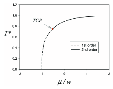
Figure 6: $T^{*}$ vs. $\mu/w$ mean field phase diagram. TCP is a tricritical point.

IV.2 Real Space Renormalization Group approach

In order to obtain a more accurate analytical prediction for the phase diagram we apply the Real Space Renormalization Group (RSRG) scheme introduced by Niemeijer and van Leeuwen NiVa1982 , using four spin Kadanoff blocks and a double majority rule RG projection matrix. The details of the RSRG implementation are given in the supplementary material SM . The application of a truncation scheme allowed us to restrict the proliferation of interactions. Under this framework, closed recursion RG relations can be obtained for the the more general Hamiltonian compatible with the basic symmetry of the system, namely, a 90 degrees rotation of the lattice when $S_{i}\to-S_{i}$, that is

$${\cal H}_{RG} = h\sum_{i}S_{i}^{2}+\sum_{<i,j>}\left[L\,S_{i}S_{i}+M\,S_{i}^{2}S_{j}^{2}\right]$$ (16)

$$+\sum_{<i,j>}\left[U\,(S_{i}^{2}S_{j}+S_{j}^{2}S_{i})\left(\hat{y}.\vec{r}_{ij}-\hat{x}.\vec{r}_{ij}\right)\right]$$

where ${\cal H}\equiv-\beta H$ and $h\equiv\beta\mu$. For $U=0$ the Hamiltonian (24) corresponds to the BEG model BlEmGr1971 . For $L=M=U=\beta w/4$ we recover the model (2).

The RG flow starting from the subspace $(L,M,U,h)=(K/4,K/4,K/4,h)$, with $K\equiv\beta w$, is governed by the following fixed points. (i) Two attractors at $I_{\pm}=(0,0,0,\pm\infty)$. They represent the high ($\left<S_{i}^{2}\right>\approx 1$) and the low ($\left<S_{i}^{2}\right>\ll 1$) density isotropic phases respectively. (ii) One semi-unstable fixed point $T_{1}=(0,0,0,-\ln 2)$. It is the locus of a surface in the $(L,M,U,h)$ space that corresponds to a smooth continuation at high temperatures between both phases. (iii) A line of attractive fixed points at $(+\infty,0,0,+\infty)$. It is the locus of the ferromagnetic phase in the whole $(L,M,U,h)$ space and we call it the $N$ attractor. (iv) One non-trivial fixed point $C_{1}=(L_{c},0,0,+\infty)$ with $L_{c}=\frac{1}{4}\,\ln\left[1+2\sqrt{2}+\sqrt{10+5\sqrt{2}}\,\right]\approx 0.518612$. It is the locus of a critical surface and corresponds to the critical point of the Ising model in the square lattice under the present approximation. The associated critical exponent results $\nu=1.0013...$, in excellent agreement with the exact result $\nu=1$. The details of this analysis are given in the supplementary material SM .

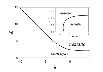
Figure 7: RG phase diagram in the $(K,h)$ space. The black continuous line is attracted by the fixed point $C_{1}$ and therefore corresponds to a secondorder critical one. The grey dashed line is attracted by the fixed point $T_{1}$ and corresponds to a smooth continuation between the high and low density isotropic phases. The inset shows the corresponding phase diagram in the $(\mu/w,T^{*})=(h/K,1/K)$ space.

The phase diagram in the $(K,h)$ space, obtained from the RG flow starting with $(L,M,U,h)=(K/4,K/4,K/4,h)$, is shown in Fig. 7. We found a single critical line separating the nematic and isotropic phases (black continuous line in Fig. 7), which is in the basin of attraction of the fixed point $C_{1}$. The nematic phase is in the basin of of attraction of $N$, while the isotropic phase is attracted either by $I_{+}$ or by $I_{-}$. Points along the grey dashed line in Fig. 7 are attracted by the trivial fixed point $T_{1}$, thus corresponding to a smooth continuation from low to high density isotropic phases, without phase transition. This line converges asymptotically to the critical line when $h\to-\infty$. Therefore, according to the present RG prediction the transition is second order for any finite temperature and it is in the universality class of the Ising model. The corresponding phase diagram in the $(\mu/w,T^{*})=(h/K,1/K)$ space is shown in the inset of Fig. 7.

Finally, to calculate the phase diagram in the $(\theta,T^{*})$ space we computed numerically the coverage $\theta(h)$ along the critical line $K_{c}=K_{c}(h)$ of Fig. 7. The results are presented in Fig. 8 and the details of the calculation are given in the supplementary material SM .

IV.3 Comparison Between Theoretical and Simulated Results

In Fig. 8 we compare the critical lines obtained by MC (open squares joined by lines) and RSRG (solid circles), together with the analytical approximation developed by Tavares et al. Tavares (solid line). While qualitatively similar to the MC result, we see that the present RSRG approximation systematically underestimates the critical temperature. Concerning the comparison with Tavares et al. results Tavares , quantitative and qualitative differences have been found between the analytical and the simulation data. In fact, the theory overestimates the critical temperature in all range of coverage, confirming the predictions in Ref. [Tavares, ]. For small values of $\theta$, small differences appear between simulation and theoretical results; however, the disagreement turns out to be significantly large for larger $\theta$’s.

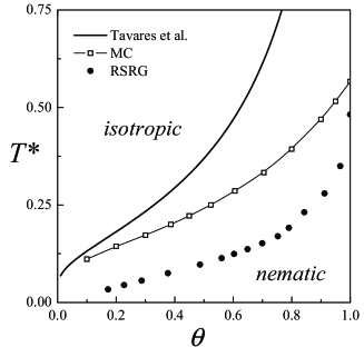
Figure 8: Comparison between numerical and theoretical estimates of the phase diagram in the $(\theta,T^{*})$ phase diagram.

In the particular case of $\theta=1$, the Tavares et al. theory predicts a critical temperature of $T^{*}_{c}=[\ln(3/2)]^{-1}\approx 2.466$, whereas the value calculated by MC simulations is $T^{*}_{c}=0.567(2)$. These results can be compared with the exact value of the critical temperature at full coverage $T^{*}_{c}=-\left[2\ln\left(\sqrt{2}-1\right)\right]^{-1}\approx 0.567$, (see section II). This result is consistent with that calculated by MC simulations, which reinforces the robustness of the present computational scheme.

V Conclusions

In summary, we have addressed the temperature-coverage phase diagram of self-assembled rigid rods on square lattices. By using Monte Carlo simulations, mean-field theory and a renormalization group approach, we obtained and characterized the critical line which separates regions of isotropic and nematic stability. Several conclusions can be drawn from the present results.

First, a simulation test of the theory developed by Tavares et al. Tavares was carried out. The results showed that the theory overestimates the critical temperature in all range of coverage, confirming the predictions in Ref. [Tavares, ]. For small values of $\theta$, small differences appear between simulation and theoretical results; however, the disagreement turns out to be significantly large for larger $\theta$’s. On the other hand, the RSRG approach reproduces qualitatively the shape of the critical line, but systematically underestimates the critical temperature. Concerning this last calculation, the main prediction is that the critical properties of the whole line are associated to a unique second-order fixed point, confirming the continuous nature of the transition. However, it must be pointed out that it predicts that the whole line is in the universality class of the $d=2$ ferromagnetic Ising model, at variance with Monte Carlo numerical calculations predicting that the transition at $\theta\approx 1/2$ belongs to the $q=1$ Potts universality class PRE4 . While the present RSRG results are not conclusive, due to the approximate character of the approach, they indicate that further research is required to clarify this point.

On the other hand, the behavior of the order parameter allowed to discard the existence of a reentrant nematic transition at high densities as speculated in Ref. [Tavares, ]. This finding indicates a substantial difference between the present system and that of monodisperse rigid rods without self-assembly, where a second nematic to isotropic phase transition is observed at high densities Ghosh ; JSTAT1

Concerning the MF results, the prediction of a first-order transition line and a tricritical point is not surprising, due to the close relationship between the present model and the BEG one, as evidenced by the Eq. (2). Indeed, the generalized form (24) contains both first-order and tricritical fixed points, but the RSRG results show that in $d=2$ the anisotropic character of the interactions drive the RG flow of the present system outside their basins of attraction. However, in three dimensional systems the IN transition is usually first-order Onsager . On the other hand, from the exact mapping into the isotropic Ising model at full coverage one could expect a second-order transition for high values of the coverage, even in three dimensions. Hence, the MF prediction of a tricritical point is probably correct for $d>2$.

Supplementary information

Here we provide the details of the RSRG calculations presented in the manuscript.

RSRG Method

Consider the Kadanoff blocks of size $N_{b}=b^{2}=4$ shown in Fig. 9. Let’s denote by $S_{I}^{\prime}$ the block spin associated to the block $I$ and $s_{I}$ the set of lattice spins belonging to the block $I$: $s_{I}\equiv\{s_{i}\}\;\;$ with $\;\;i\in I$. Let’s also denote by $S^{\prime}$ and $s$ the complete sets of block and lattice spins respectively. We can express ${\cal H}={\cal H}_{0}+{\cal V}$, where ${\cal H}_{0}=\sum_{I}{\cal H}_{I}(s_{I})$ contains all the interactions between spins belonging to the block $I$ and $\cal V$ all the interblock interactions. Introducing an RG projection matrix $P(S^{\prime},s)=\prod_{I}P_{I}(S_{I}^{\prime},s_{I})$, an average of an arbitrary function $X(S^{\prime},s)$ as

$$\left<X\right>_{0}(S^{\prime})\equiv\frac{1}{Z_{0}}\;\sum_{s}P(S^{\prime},s)e^{{\cal H}_{0}(s)}X(S^{\prime},s)$$ (17)

where $Z_{0}=\prod_{I}Z_{0}^{I}$ with

$$Z_{0}^{I}(S_{I})=\sum_{s_{I}}P_{I}(S_{I}^{\prime},s_{I})e^{{\cal H}_{I}(s_{I})}$$

The simplest RG approach within Niemeijer and van Leeuwen NiVa1982 scheme consist into the identification

$${\cal H}^{\prime}(S^{\prime})+{\cal C}=\ln Z_{0}+\left<V\right>_{0},$$ (18)

where ${\cal H}^{\prime}(S^{\prime})$ is the block Hamiltonian and ${\cal C}$ is a spin-independent constant. This uncontrolled approximation results from the truncation to the first-order cumulantNiVa1982 of $\left<\exp(V)\right>_{0}$. Using then of the double majority rule RG projection matrix $P_{I}(S_{I}^{\prime},s_{I})$ introduced by Berker and Wortis for the pure isotropic Blume-Emery-Griffiths (BEG) model BeWo1976 , it is easy to see that $\left<S_{iI}\right>_{0}=a_{1}\,S_{I}^{\prime}$, $\left<S_{iI}^{2}\right>_{0}=a_{2}\,S_{I}^{\prime 2}+a_{3}$, and $\ln Z_{0}^{I}=a_{4}S_{I}^{\prime 2}+a_{5}$, where

$$a_{1} = \left.\left<S_{iI}\right>_{0}\right|_{S_{I}^{\prime}=1}$$ (19)

$$a_{2} = \left.\left<S_{iI}^{2}\right>_{0}\right|_{S_{I}^{\prime}=1}-\left.\left<S_{iI}^{2}\right>_{0}\right|_{S_{I}^{\prime}=0}$$ (20)

$$a_{3} = \left.\left<S_{iI}^{2}\right>_{0}\right|_{S_{I}^{\prime}=0}$$ (21)

$$a_{4} = \left.\ln Z_{0}^{I}\right|_{S_{I}^{\prime}=1}-\left.\ln Z_{0}^{I}\right|_{S_{I}^{\prime}=0}$$ (22)

$$a_{5} = \ln\left.Z_{0}^{I}\right|_{S_{I}^{\prime}=0}.$$ (23)

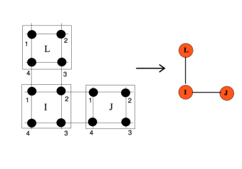
Figure 9: Kadanoff blocks of size $b=2$ for the square lattice.

Applying this scheme to the Hamiltonian

$${\cal H}_{RG} = h\sum_{i}S_{i}^{2}+\sum_{<i,j>}\left[L\,S_{i}S_{i}+M\,S_{i}^{2}S_{j}^{2}\right.$$ (24)

$$+\left.U\,(S_{i}^{2}S_{j}+S_{j}^{2}S_{i})\left(\hat{y}.\vec{r}_{ij}-\hat{x}.\vec{r}_{ij}\right)\right],$$

we obtain the closed RG recursion relations

$$L^{\prime} = 2L\,a_{1}^{2}$$ (25)

$$M^{\prime} = 2M\,a_{2}^{2}$$ (26)

$$U^{\prime} = 2U\,a_{1}a_{2}$$ (27)

$$h^{\prime} = 8M\,a_{2}\,a_{3}+a_{4},$$ (28)

together with

$$g={\cal C}/N=(M\,a_{3}^{2}+a_{5}/4).$$ (29)

Defining

$$B_{1}(L,M,U,h) = \left.Z_{0}^{I}\right|_{S_{I}^{\prime}=0}$$

$$B_{2}(L,M,U,h) = \left.Z_{0}^{I}\right|_{S_{I}^{\prime}=1}$$

we obtain

$$a_{3} = \frac{2\,e^{h}+2\,e^{2h}+2\,e^{2h+M-L}+2\,e^{2h+M+L}\cosh(2U)}{B_{1}(L,M,U,h)}$$

$$a_{4} = \ln\frac{B_{2}(L,M,U,h)}{B_{1}(L,M,U,h)}$$

$$a_{5} = \ln B_{1}(L,M,U,h)$$

and

$$a_{1} = \frac{1}{B_{2}(L,M,U,h)}\left[\frac{1}{2}\,e^{2h}+2\,e^{4(h+M)}+e^{3h+2(M-L)}+3\,e^{3h+2(M+L)}+e^{4(h+M+L)}+\right.$$

$$+ \left.e^{2h+M+L}\,\cosh(2U)+2\,e^{3h+2M}\,\cosh(2U)\right]$$

$$a_{2} = \frac{1}{B_{2}(L,M,U,h)}\left[e^{2h}+6\,e^{4(M+h)}+e^{2h+M-L}+6\,e^{3h+2M}\,\cosh(2L)+2\,e^{4(M+h)}\,\cosh(4L)+\right.$$

$$+ \left.e^{2h+M+L}\,\cosh(2U)+6\,e^{2M+3h}\,\cosh(2U)\right]-a_{3}(L,M,U,h)$$

$$a_{3} = \frac{2\,e^{h}+2\,e^{2h}+2\,e^{2h+M-L}+2\,e^{2h+M+L}\cosh(2U)}{B_{1}(L,M,U,h)}$$

$$B_{1} = 1+8\,e^{h}+4\,e^{2h}+4\,e^{2h+M-L}+4\,e^{2h+M+L}\,\cosh(2U)$$

$$B_{2} = 2\,e^{2h}+6\,e^{4(M+h)}+2\,e^{2h+M-L}+8\,e^{3h+2M}\,\cosh(2L)+2\,e^{4(M+h)}\,\cosh(4L)+$$

$$+ 2\,e^{2h+M+L}\,\cosh(2U)+8\,e^{3h+2M}\,\cosh(2U).$$

RSRG flow and fixed points structure

We found that all the relevant fixed points of the recursion equations lie in the BEG subspace $U=0$. The RG flow and the fixed points structure in the $U=0$ subspace is qualitatively similar to that obtained in Ref. [BeWo1976, ], including first and second-order surfaces, as well as tricritical and critical endpoint lines BeWo1976 . We focused only on those fixed points relevant to the present problem namely, those which govern the RG flow starting from the subspace $(L,M,U,h)=(K/4,K/4,K/4,h)$, with $K\equiv\beta w$. The whole flow starting from that subspace is attracted by two subspaces invariant under RG: $L=M=U=0$ and $(M,h)=(0,+\infty)$.

Flow in the $L=M=U=0$ subspace

The recursion relations in this case reduce to $h^{\prime}=a_{4}(0,0,0,h)$. This RG equation presents three fixed points: two attractors at $h=\pm\infty$, which are the loci of the high ($h=\infty$) and low ($h=-\infty$) density isotropic phases respectively and one unstable high temperature fixed point at $h=-\ln 2$. The first two fixed points are attractors in the complete $(L,M,U,h)$ space and we will call them $I_{+}$ and $I_{-}$. They represent the high ($\left<S_{i}^{2}\right>\approx 1$) and the low ($\left<S_{i}^{2}\right>\ll 1$) density isotropic phases respectively. The fixed point $T_{1}\equiv(0,0,0,-\ln 2)$ is the locus of a surface in the $(L,M,U,h)$ space that corresponds to a smooth continuation at high temperatures between both phases.

Flow in the $(M,h)=(0,+\infty)$ subspace

This subspace corresponds to an anisotropic Ising model, since in this limit the $S_{i}=0$ state has zero probability. The recursion relations reduce in this case to

$$L^{\prime} = 2L\,d(L)^{2}$$ (30)

$$U^{\prime} = Ud(L)$$ (31)

with

$$d(L)=\lim_{h\to\infty}a_{1}(L,0,U,h)=\frac{2+e^{4L}}{6+2\,\cosh(4L)}.$$ (32)

Since $L^{\prime}=L^{\prime}(L)$, independently of the parameter $U$, the whole flow is governed by the RG equation corresponding to the isotropic Ising model. This equation has a non trivial fixed point at $d(L)=1/\sqrt{2}$, whose solution is $L_{c}=\frac{1}{4}\,\ln\left[1+2\sqrt{2}+\sqrt{10+5\sqrt{2}}\,\right]\approx 0.518612$, corresponding to the critical point of the Ising model in the square lattice under the present approximation (compare with exact Onsager result $L_{c}=\frac{1}{2}\ln(1+\sqrt{2})\approx 0.44069$). We will call this fixed point $C_{1}$. The critical exponent $\nu$ is given by

$$\nu=\frac{\ln b}{\ln\lambda}\;\;\;\;\lambda=\left.\frac{\partial L^{\prime}}{\partial L}\right|_{L_{c}}.$$

We obtain $\nu=1.0013...$, in excellent agreement with the exact result $\nu=1$. The RG recursion equation also has two attractors: $I_{+}$ ($L=0$) and the isotropic ferromagnetic fixed point $L=\infty$ ($T=0$). At $L=L_{c}$ we have another invariant line at the $(L,U)$ space, whose RG equation is $U^{\prime}=U^{\prime}/\sqrt{2}$. This recursion relation has only trivial fixed points: one attractor at $U=0$ and one unstable at $U=+\infty$. The line $L=0$ is also invariant and have the same fixed points. Finally, we have that $\lim_{L\to\infty}d(L)=1$ Hence, $U^{\prime}=U$ and the whole line $L=+\infty$ is a line of fixed points. This is the locus of the ferromagnetic phase in the whole $(L,M,U,h)$ space and we will call it the $N$ attractor. In Fig. 10 we show the flow diagram in the complete $(U,L)$ space.

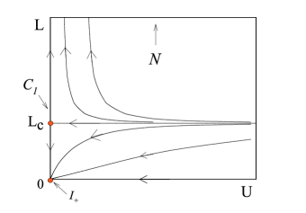
Figure 10: RG flow in the $(L,0,U,+\infty)$ invariant subspace.

RSRG Coverage calculation

The coverage can be expressed as

$$\theta(K,h)=-\beta\frac{\partial f(K,h)}{\partial h}.$$ (33)

Let $\vec{K}\equiv(L,M,U,h)$ be the parameters vector of Hamiltonian (24). From the renormalization group transformation we have the following relation after $n$ applications of the RG transformation NiVa1982

$$f(\vec{K}_{0})=-\frac{1}{\beta}\sum_{m=0}^{n}b^{-md}g(\vec{K}_{m})+b^{-nd}f(\vec{K}_{n}),$$ (34)

where $\vec{K}_{m}$ is the parameters vector after $m$ applications of the RG transformation, $\vec{K}_{0}$ is the initial value and $g(\vec{K})={\cal C}/N$ is given by Eq. (29). Since $\theta$ is not singular at the critical line, we can assume that the singular part of the free energy will make no contribution to Eq. (34) and therefore the derivative of the second term in the right hand of the previous expression vanishes when $n\to\infty$. Therefore, we can express

$$\theta(K,h)=\frac{\partial}{\partial h}\left[\sum_{m=0}^{\infty}b^{-md}g(\vec{K}_{m})\right]_{\vec{K}_{0}=(K/4,K/4,K,4,h)}.$$ (35)

Computing numerically the above sum and taking the numerical derivative we obtain the critical line $T^{*}$ vs. $\theta$ shown in Fig. 8 of the manuscript.

References

- (1) T. Niemeijer and J. M. J. van Leeuwen, Phase Transition and Critical Phenomena, 6, C. Domb and M. S. Green (eds.) (Springer-Verlag, New York, 1982).
- (2) A. N. Berker and M. Wortis, Phys. Rev. B 14, 4946 (1976).