Linear-response theory of spin Seebeck effect
in ferromagnetic insulators
Hiroto Adachi
hiroto.adachi@gmail.com
Advanced Science Research Center, Japan Atomic Energy Agency,
Tokai 319-1195, Japan
CREST, Japan Science and Technology Agency, Sanbancho, Tokyo 102-0075, Japan
Jun-ichiro Ohe
Advanced Science Research Center, Japan Atomic Energy Agency,
Tokai 319-1195, Japan
CREST, Japan Science and Technology Agency, Sanbancho, Tokyo 102-0075, Japan
Saburo Takahashi
Institute for Materials Research,
Tohoku University, Sendai 980-8577, Japan
CREST, Japan Science and Technology Agency, Sanbancho, Tokyo 102-0075, Japan
Advanced Science Research Center, Japan Atomic Energy Agency,
Tokai 319-1195, Japan
Sadamichi Maekawa
Advanced Science Research Center, Japan Atomic Energy Agency,
Tokai 319-1195, Japan
CREST, Japan Science and Technology Agency, Sanbancho, Tokyo 102-0075, Japan
Abstract
We formulate a linear response theory of the spin Seebeck effect, i.e.,
a spin voltage generation from heat current flowing in a ferromagnet.
Our approach focuses on the collective magnetic excitation of
spins, i.e., magnons.
We show that the linear-response formulation provides us with
a qualitative as well as quantitative understanding of
the spin Seebeck effect observed in a prototypical magnet,
yttrium iron garnet.
pacs:
85.75.-d, 72.15.Jf, 72.25.-b
I Introduction
The generation of spin voltage, i.e., the potential for an electron’s spin
to drive spin currents, by a temperature gradient in a ferromagnet
is referred to as the spin Seebeck effect (SSE).
Since the first observation of the SSE in a
ferromagnetic metal Ni81Fe19, Uchida08
this phenomenon has attracted much attention
as a new method of generating spin currents from heat energy
and opened a new possibility of spintronics devices. Zutic04
The SSE triggered the emergence of the new field dubbed
“spin caloritronics” SpinCalo ; Slonczewski in the
rapidly growing spintronics community.
Moreover, as the induced spin voltage can be converted into electric
voltage through the inverse spin Hall effect Saitoh06
at the attached nonmagnetic metal, this phenomenon put a new twist
on the long and well-studied history of thermoelectric research. Blatt76
One of the canonical frameworks to describe nonequilibrium transport
phenomena is linear-response theory. Mahan-text
Having been applied to a number of transport phenomena,
linear-response theory has been so successful
because it is intimately related
to the universal fluctuation-dissipation theorem.
Up to now, however, the linear-response formulation of the SSE has not
been known mainly because, unlike the charge current,
the spin current is not a conserved quantity.
Therefore, it is of great importance to formulate the SSE in terms
of linear-response theory.
Concerning the SSE, a big mystery is now being established, which is,
how can conduction electrons sustain the spin voltage over
such a long range of several millimeters Uchida08
in spite of the conduction electrons’ short spin-flip
diffusion length, which is typically of several tens of nanometers?
A key to resolve this puzzle was reported by
a recent experiment on electric signal transmission through
a ferromagnetic insulator Kajiwara10
which demonstrates that the spin current can be carried by
the low-lying magnetic excitation of localized spins, i.e.,
the magnon excitations, and that it can transmit the spin current
as far as several millimeters.
Subsequently, the SSE was reported to be observed in the
magnetic insulator LaY2Fe5O12 despite the absence of
conduction electrons. Uchida10 These experiments suggest that
contrary to the conventional wisdom over the last two decades that
the spin current is carried by conduction electrons, Maekawa06
the magnon is a promising candidate as a carrier for the SSE.
The purpose of this paper is twofold. First, we analyze the SSE
observed in LaY2Fe5O12Uchida10
(hereafter referred to as YIG) in terms of magnon spin current,
i.e., a spin current carried by magnon excitations.
Second, we develop a framework for analyzing the SSE
by means of the standard linear-response formalism Mahan-text
which is amenable to the language of the magnetism community. Simanek03
This allows us to describe the spin transport phenomena
systematically, and it can be easily generalized
to a situation including degrees of freedom other than magnons,
e.g., conduction electrons and phonons,
to describe a more complicated process in the case of
metallic systems. Uchida08
The plan of this paper is as follows.
In Sec. II, we present a linear-response
approach to the “local” spin injection by thermal magnons,
in which the spin injection is driven by the temperature
difference between the ferromagnet and the attached nonmagnetic metal.
Next, in Sec. III we develop a linear-response
theory of the “nonlocal” spin injection by thermal magnons,
in which the spin injection is driven by the temperature
gradient inside the ferromagnet.
As one can see below, this process can explain the SSE observed
in YIG. Uchida10
Finally, in Sec. IV we summarize and discuss our results.
II “Local” spin injection by thermal magnons
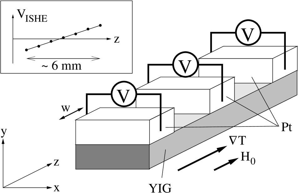
Figure 1: Experimental setup for observing the SSE. Uchida10
Inset: Schematics of the spatial profile of the observed voltage.
We start by briefly reviewing the SSE experiment for YIG. Uchida10
Figure 1 shows the experimental setup
where several Pt terminals are attached on top of a YIG film in
a static magnetic field ( anisotropy field)
which aligns the localized magnetic moment along .
A temperature gradient
is applied along the axis, and it
induces a spin voltage across the YIG/Pt interface.
This spin voltage then injects a spin current into the Pt terminal
(or ejects it from the Pt terminal).
A part of the injected/ejected spin current is converted
into a charge voltage
through the so-called inverse spin Hall effect: Saitoh06
(1)
where , , , and are
the absolute value of electron charge, spin Hall angle, resistivity,
and width of the Pt terminal (see Fig. 1),
respectively. Hence, the observed charge voltage
is a measure of the injected/ejected spin current .
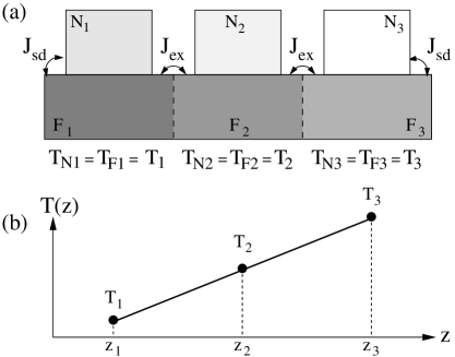
To investigate the SSE observed in YIG, we consider a model
shown in Fig. 2(a).
While YIG is a ferrimagnet, we model it as a ferromagnet
since we are interested in the low-energy properties.
The key point in our model is that the temperature gradient
is applied over the insulating ferromagnet, but there is locally
no temperature difference between the ferromagnet and
the attached nonmagnetic metals, i.e., ,
, and .
We assume that each domain is initially in thermal equilibrium
without interactions with the neighboring domains, and then calculate
the nonequilibrium dynamics after we switch on the interactions.
Note that this procedure is essentially equivalent to that
used by Luttinger Luttinger64 to realize the initial condition
mentioned above.
Let us consider first the low-energy excitations
in the ferromagnet. In the following, we focus on the spin-wave region
where the magnetization
fluctuates only weakly around the ground state value
with the saturation magnetization ,
and we set
to separate the small fluctuation part
from the ground state value.
Then, the low-energy excitations of are described by
boson (magnon) operators and
through the relations Akhiezer60
and
where , is the
size of localized spins, and
with being the number of localized spins in the ferromagnet.
Consistent with this boson mapping, the magnetization dynamics
is described by the following action: Doniach74 ; Schmid82
(2)
where the integration is performed along the Keldysh contour , Rammer86
and the bare magnon propagator is given by
(3)
with the following equilibrium condition:
(4)
The retarded component of is given by
where is the Gilbert damping constant,
and
is the magnon frequency.
Here, is the gyromagnetic ratio and
,
where is the spin-wave stiffness constant
with and
being the exchange energy and the effective block spin volume.
In the nonmagnetic metal, the dynamics of the spin density
can be described by the action Hertz74
(5)
where
is defined by
with ,
,
and
being the Pauli matrices,
the electron creation operator for spin projection
and , and the number of atoms
in the nonmagnetic metal.
The equilibrium spin-density propagator is given by
(6)
with the following equilibrium condition:
(7)
The retarded part of is given by Fulde68
with , , and being
the paramagnetic susceptibility, spin diffusion length,
and spin relaxation time, the form of which is consistent
with the corresponding diffusive Bloch equation [see Eq. (10) below].
Finally, the interaction between magnons and spin density at the interface
is given by
(8)
where is the Fourier
transform of
with being the - exchange interaction
between conduction-electron spins and localized spins, and
.
Figure 2: (a) System composed of ferromagnet
() and nonmagnetic metals () divided into the three temperature
domains of , , and with their local
temperatures of , , and .
(b) Temperature profile.
It is instructive to point out that in the spin-wave region
and in the classical limit
with negligible quantum fluctuations,
a system described by Eqs. (2), (5), and (8)
is equivalent Dominicis75 ; Schmid82
to a system described by the stochastic
Landau-Lifshitz-Gilbert equation,
where ,
is the diffusion constant, and
is the spin accumulation with the local equilibrium spin density
.
The noise field represents
thermal fluctuations in
with
and
, Brown63
while the noise source in
satisfies and
Ma75
with the lattice constant ,
both of which are postulated by the fluctuation-dissipation theorem.
In this section we focus on the “local” spin injection from into .
The spin current induced in can be calculated
from the linear response expression of the
magnon-mediated spin injection given in the Appendix A
[Eq. (26)].
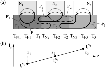
Consider the process shown in Fig. 3 (a)
where magnons travel around the ferromagnet without feeling
the temperature difference between and .
Using the standard rules of constructing the
Feynman diagram in Keldysh space, Rammer86
the corresponding interface Green’s function
for the correlation
between the magnons in and the spin density in
[Eq. (26)] can be written in the form
(11)
where and are the number of lattice sites
in and .
Substituting Eq. (11) into Eq. (26)
and employing the equilibrium conditions
[Eqs. (4) and (7)],
we obtain the expression for the injected spin current
(12)
where we have introduced the shorthand notation
,
and is the number of localized spins at the - interface
playing a role of the number of channels.
The integration can be performed by picking up
only magnon poles under the condition
(always satisfied
for YIG), giving
.
By making the classical approximation
,
we obtain
(13)
where
with the dimensionless variables
and ,
and we used the relation
.
III Magnon-mediated spin Seebeck effect
Equation (13) means that, through the “local” process
shown in Fig. 3(a),
the spin current is not injected
into the nonmagnetic metal
when and have the same temperature.
That is, the “local” process cannot
explain the experiment Uchida10 where
no temperature difference exists between the YIG film
and the attached Pt film.
A way to account for the experiment within the “local” picture
is to invoke a difference between the phonon temperature and magnon
temperature. Xiao10
In this paper, on the other hand, we take a different route
and consider the effect of temperature gradient within the YIG film
on the spin injection into the Pt terminal.
The basic idea of our approach is as follows.
The above result [Eq. (13)] that the injected spin current
vanishes when originates from the equilibrium condition
of the magnon propagator [Eq. (4)]. When magnons deviate from
local thermal equilibrium by allowing the magnons to feel the temperature
gradient inside the ferromagnet, the magnon propagator cannot be written in
the equilibrium form, and it generates a nontrivial contribution
to the thermal spin injection.
The relevant “nonlocal” process is shown in Fig. 3(a)
in which magnons feel the temperature difference between and .
The interaction between and is described by the action
(14)
where is the Fourier
transform of
with .
Figure 3: (a) Feynman diagrams expressing the spin current
injected from the ferromagnet () to the nonmagnetic metals ().
The thin solid lines with arrows (bold lines without arrows)
represent electron propagators (magnon propagators).
(b) Spatial profile of the calculated spin current.
We now regard the whole of the magnon lines
appearing in the process as a single magnon propagator
, namely,
(15)
Then the propagator is decomposed into the local-equilibrium part
and nonequilibrium part as Michaeli09
(16)
where
(17)
is the local-equilibrium propagator satisfying the
local-equilibrium condition, i.e.,
and
with
(18)
while
(19)
is the nonequilibrium propagator
with given by
(20)
Note that the local equilibrium propagator [Eq. (17)]
does not contribute to the “nonlocal” spin injection.
When we substitute Eq. (16) into
Eq. (26) and use Eq. (11) with
being replaced by ,
we obtain the following expression for the
magnon-mediated thermal spin injection:
(21)
where is the number of localized
spins at the - interface, and we used
.
The integration can be performed as before, giving
, which suggests that the magnon
modes with different ’s do not interfere with each other.
With the classical approximation
, we obtain
(22)
where ,
is the size of along the temperature gradient,
and
which is approximated
as
()
for
(for ).
The spin current injected into the right terminal
can be calculated in the same manner by considering the process ,
which gives
from the relation .
The spin current
injected into the middle terminal vanishes
because the two relevant processes ( and ) cancel out.
Therefore, we obtain the spatial profile of the injected spin current
as shown in Fig. 3(b).
Note that the effect of the spatial dependence of magnetization
through the local temperature
is already taken into account in our treatment because the temperature
dependence of in the magnon region
is automatically described by the number of thermal magnons
discussed in this paper.
For an order of magnitude estimation,
we compare Eq. (22) with the experiment. Uchida10
By using , Kimura07 ; Hoffmann10
,
,
,
,
,
,
,
, Kajiwara10
, Kriessman54
and ,
the - exchange coupling extracted from the previous ferromagnetic resonance
experiment Kajiwara10 ()
can account for the spin Seebeck voltage
observed at room temperature.
Finally, we comment on the issue of length scales associated with the SSE.
In the original SSE experiment for a metallic ferromagnet, Uchida08
the signal maintained over several millimeters was a big surprise because
the spin diffusion length for that system is much shorter than a millimeter.
Concerning the magnon-mediated SSE in an insulating
magnet Uchida10 which we have discussed,
it is of crucial importance to recognize that the length scale relevant to
the SSE is related to magnon density fluctuations and is given by
longitudinal fluctuations of magnons,
while the magnon mean free path is related to magnon dephasing
and is given by transverse fluctuations of magnons. com01
It was shown by Mori and Kawasaki Mori62
that these two length scales do not coincide with each other since
they obey quite different dynamics, and it was demonstrated that
in a certain situation the length scale of magnon density fluctuations
(which is relevant to the SSE as well) is much longer than the magnon mean free path
[see Eq.(6.33) in Ref. Mori62, where the length scale of
long-wavelength magnon density fluctuations is infinitely long]. com02
The notion of these two different length scales is the key to understanding
the length scales observed in the
SSE experiment in an insulating magnet. Uchida10
IV Conclusion
We have developed a theory of the magnon-mediated
spin Seebeck effect in terms of the canonical framework of
describing transport phenomena,
i.e., the linear-response theory,
and shown that it provides us with
a qualitative as well as quantitative understanding of
the spin Seebeck effect observed in a prototypical magnet,
yttrium iron garnet. Uchida10
Because the carriers of spin current in this scenario are magnons,
we can obtain a bigger signal for a magnetic material
with a lower magnon damping
[see Eq. (22) where the injected spin current
is inversely proportional to the Gilbert damping constant ].
An advantage of our linear-response formulation is that it can be easily
generalized to a situation including degrees of freedom other than magnons,
e.g., phonons and conduction electrons, to describe
a more complicated process in the case of metallic Uchida08 and
semiconducting systems, Jaworski10
and a calculation taking account of the effect of nonequilibrium phonons
will be reported in a future publication. Adachi-next
A numerical approach to the SSE is also developed in Ref. Ohe11, .
We believe that the present approach stimulates further research
on the spin Seebeck effect.
Acknowledgements.
We are grateful to E. Saitoh, K. Uchida, G. E. W. Bauer, and J. Ieda
for helpful discussions.
This work was financially supported by
a Grant-in-Aid for Scientific Research on Priority Areas (No. 19048009)
and a Grant-in-Aid for Young Scientists (No. 22740210) from MEXT, Japan.
Appendix A Linear-response expression of magnon-induced
spin injection
The Gaussian action for conduction electrons in the
nonmagnetic metal () is given by
(23)
where
is the electron creation operator for spin projection
and ,
is the Fourier transform of the impurity potential
,
and measures the strength of the
spin-orbit interaction. Takahashi08
At the ferromagnet/nonmagnetic-metal interface, the magnetic interaction
between conduction-electron spin density and localized spin is described
by the - interaction [Eq. (8)].
The spin current induced in the nonmagnetic metal
can be calculated as the rate of change of the spin accumulation in ,
i.e.,
,
where means the statistical average at a given time ,
and
with being defined below Eq. (5).
The Heisenberg equation of motion for gives
(24)
where we have used the relation
, and
neglected a small correction term arising from the
spin-orbit interaction assuming that
the spin-orbit interaction is weak enough
at the neighborhoods of the interface.
Then, the statistical average of the above quantity gives
the following spin current:
(25)
where
is the interface Green’s function.
In the steady state, the Green’s function
depends only on the time difference as
.
Adopting the representation Larkin75
and using ,
we finally obtain
(26)
for the spin current in a steady state.
As in the case of tunneling charge current driven by
a voltage difference, Caroli71 the spin current
can be calculated systematically.
References
(1)
K. Uchida, S. Takahashi, K. Harii, J. Ieda, W. Koshibae, K. Ando,
S. Maekawa, and E. Saitoh,
Nature 455, 778 (2008).
(2)
I. Z̆utić, J. Fabian, and S. D. Sarma,
Rev. Mod. Phys. 76, 323 (2004).
(3)Spin Caloritronics, edited by G. E. W. Bauer, A. H. MacDonald,
and S. Maekawa, special issue of Solid State Commun., 150, 459 (2010).
(4)
J. C. Slonczewski,
Phys. Rev. B 82, 054403 (2010).
(5)
E. Saitoh, M. Ueda, H. Miyajima, and G. Tatara,
Appl. Phys. Lett. 88, 182509 (2006).
(6)
F. J. Blatt, P. A. Schroeder, C. L. Foiles, and D. Greig,
Thermoelectric Power of Metals (Plenum Press, New York, 1976).
(7)
For example, G. Mahan,
Many-Particle Physics (Kluwer Academic, New York, 1981).
(8)
Y. Kajiwara, K. Harii, S. Takahashi, J. Ohe, K. Uchida, M. Mizuguchi, H. Umezawa,
H. Kawai, K. Ando, K. Takanashi, S. Maekawa, and E. Saitoh,
Nature 464, 262 (2010).
(9)
K. Uchida, J. Xiao, H. Adachi, J. Ohe, S. Takahashi, J. Ieda, T. Ota, Y. Kajiwara,
H. Umezawa, H. Kawai, G. E. W. Bauer, S. Maekawa, and E. Saitoh,
Nature Mater. 9, 894 (2010).
(10)Concepts in Spin Electronics, ed. S. Maekawa
(Oxford University Press, Oxford, U.K., 2006).
(11)
E. Šimánek and B. Heinrich,
Phys. Rev. B 67, 144418 (2003).
(12)
J. M. Luttinger, Phys. Rev. 135, A1505 (1964).
(13)
A. I. Akhiezer, V. G. Baryakhtar, and M. I. Kaganov,
Usp. Fiz. Nauk 71, 533 (1960) [Sov. Phys. Usp. 3, 567 (1961)].
(14)
S. Doniach and E. H. Sondheimer,
Green’s Functions for Solid State Physicists
(Benjamin, New York, 1974).
(15)
A. Schmid,
J. Low Temp. Phys. 49, 609 (1982).
(16)
For a review, see, e.g., J. Rammer and H. Smith,
Rev. Mod. Phys. 58, 323 (1986).
(17)
J. A. Hertz and M. A. Klenin,
Phys. Rev. B 10, 1084 (1974).
(18)
P. Fulde and A. Luther,
Phys. Rev. 175, 337 (1968).
(19)
C. De. Dominicis, Nuovo Cimento Lett. 12, 567 (1975).
(20)
S. Zhang and Z. Li,
Phys. Rev. Lett. 93, 127204 (2004).
(21)
W. F. Brown, Jr., Phys. Rev. 130, 1677 (1963).
(22)
S. Ma and G. F. Mazenko,
Phys. Rev. B 11, 4077 (1975).
(23)
J. Xiao, G. E. W. Bauer, K. Uchida, E. Saitoh, and S. Maekawa,
Phys. Rev. B 81, 214418 (2010).
(24)
K. Michaeli and A. M. Finkel’stein,
Phys. Rev. 80, 115111 (2009).
(25)
T. Kimura, Y. Otani, T. Sato, S. Takahashi, and S. Maekawa,
Phys. Rev. Lett. 98, 156601 (2007).
(26)
O. Mosendz, J. E. Pearson, F. Y. Fradin, G. E. W. Bauer,
S. D. Bader, and A. Hoffmann,
Phys. Rev. Lett. 104, 046601 (2010).
(27)
C. Kriessman and H. Callen,
Phys. Rev. 94, 837 (1954).
(28)
Note that our scenario does not rely on the long propagation length
of dipole magnons ( several millimeters) observed in
Ref. Schneider08, ,
since the magnons which we have discussed here are of exchange origin.
(29)
T. Schneider, A. A. Serga, B. Leven, B. Hillebrands,
R. L. Stamps, and M. P. Kostylev,
Appl. Phys. Lett. 92, 022505 (2008).
(30)
H. Mori and K. Kawasaki,
Prog. Theor. Phys. 27, 529 (1962).
(31)
An analogous situation occurs for conduction electrons in a disordered
metal Vollhardt80 where the length scale associated with the
long-wavelength density fluctuations of conduction electrons is infinite
due to the charge conservation while that related to the dephasing
of conduction electrons, i.e., the mean free path of conduction electrons,
is as short as several nanometers.
(32)
D. Vollhardt and P. Wölfle,
Phys. Rev. B 22, 4666 (1980).
(33)
C. M. Jaworski, J. Yang, S. Mack, D. D. Awschalom, J. P. Heremans, and
R. C. Myers,
Nature Mater. 9, 898 (2010).
(34)
H. Adachi, K. Uchida, E. Saitoh, J. Ohe, S. Takahashi, and S. Maekawa,
Appl. Phys. Lett. 97, 252506 (2010).
(35)
J. Ohe, H. Adachi, S. Takahashi, and S. Maekawa,
Phys. Rev. B 83, 115118 (2011).
(36)
S. Takahashi and S. Maekawa,
J. Phys. Soc. Jpn 77, 031009 (2008).
(37)
A. I. Larkin and Yu. N. Ovchinnikov,
Zh. Eksp. Teor. Fiz. 68, 1915 [Sov. Phys. JETP 41, 960 (1976)].
(38)
C. Caroli, R. Combescot, P. Nozieres, and D. Saint-James,
J. Phys. C: Solid State Phys. 4, 916 (1971).