Present address: ]Laboratoire FAST, CNRS UMR 7608, Université Paris-Sud, 91405 Orsay, France

Experimental evidence of a phase transition in a closed turbulent flow

Abstract

We experimentally study the susceptibility to symmetry breaking of a closed turbulent von Kármán swirling flow from $Re=150$ to $Re\simeq 10^{6}$. We report a divergence of this susceptibility at an intermediate Reynolds number $Re=Re_{\chi}\simeq 90\,000$ which gives experimental evidence that such a highly space and time fluctuating system can undergo a “phase transition”. This transition is furthermore associated with a peak in the amplitude of fluctuations of the instantaneous flow symmetry corresponding to intermittencies between spontaneously symmetry breaking metastable states.

Phase transitions are ubiquitous in physical systems and generally are associated to symmetry breakings. For example, ferromagnetic systems are well known to undergo a phase transition from paramagnetism to ferromagnetism at the Curie temperature $T_{c}$. This transition is associated with a symmetry breaking from the disordered paramagnetic —associated to a zero magnetization— toward the ordered ferromagnetic phase —associated to a finite magnetization— landau . In the vicinity of $T_{c}$, a singular behaviour characterized by critical exponents is observed, e.g. for the magnetic susceptibility to an external magnetic field. In the context of fluid dynamics, symmetry breaking also governs the transition to turbulence, that usually proceeds, as the Reynolds number $Re$ increases, through a sequence of bifurcations breaking successively the various symmetries allowed by the Navier-Stokes equations coupled to the boundary conditions manneville . Finally, at large Reynolds number, when the fully developed turbulent regime is reached, it is commonly admitted that all the broken symmetries are restored in a statistical sense, the statistical properties of the flow not depending anymore on $Re$ frisch . However, recent experimental studies of turbulent flows have disturbed this vision raising intriguing features such as finite lifetime turbulence hof —questioning the stability of the turbulent regime— and possible existence of turbulent transitions castaing ; mujica ; lohse2009 ; tabeling96 ; tabeling02 ; ravelet2004 ; ravelet2008 . Consequently, despite turbulent flows are intrinsically out-of-equilibrium systems, one may wonder whether the observed transitions can be interpreted in terms of phase transitions with a symmetry-breaking or susceptibility divergence signature. In this paper, we introduce a susceptibility to symmetry breaking in a von Kármán turbulent flow and investigate its evolution as $Re$ increases from $150$ to $10^{6}$ using stereoscopic Particle Image Velocimetry (PIV). We observe a divergence of susceptibility at a critical Reynolds number $Re=Re_{\chi}\simeq 90\,000$ which sets the threshold for a possible turbulent “phase transition”. Moreover, this divergence is associated with a peak in the amplitude of the fluctuations of the flow instantaneous symmetry.

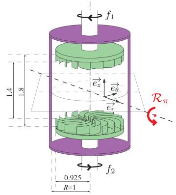
Figure 1: Schematic view of the experimental setup and the impellers blade profile. The arrow on the shaft indicates the impeller rotation sense studied. Symmetry : the system is symmetric regarding any $\cal{R}_{\pi}$-rotation of angle $\pi$ around any line of the equatorial plane which crosses the rotation axis.

Our experimental setup consists of a Plexiglas cylinder of radius $R=100$ mm filled up with either water or water-glycerol mixtures. The fluid is mechanically stirred by a pair of coaxial impellers rotating in opposite sense (Fig. 1). The impellers are flat disks of radius $0.925\,R$, fitted with 16 radial blades of height $0.2\,R$ and curvature radius $0.4625\,R$. The disks inner surfaces are $1.8\,R$ apart setting the axial distance between impellers from blades to blades to $1.4\,R$. The impellers rotate, with the convex face of the blades pushing the fluid forward, driven by two independent brushless 1.8 kW motors. The rotation frequencies $f_{1}$ and $f_{2}$ can be varied independently from $1$ to $12$ Hz. Velocity measurements are performed with a stereoscopic PIV system provided by DANTEC Dynamics. The data provide the radial $u_{r}$, axial $u_{z}$ and azimuthal $u_{\varphi}$ velocity components in a meridian plane on a 95$\times$66 points grid with $2.08$ mm spatial resolution through time series of $400$ to $27\,000$ fields regularly sampled, at frequencies from 1 to 15 Hz, depending on the turbulence intensity and the related need for statistics. The control parameters of the studied von Kármán flow are the Reynolds number $Re=\pi(f_{1}+f_{2})R^{2}/\nu$, where $\nu$ is the fluid viscosity, which controls the intensity of turbulence and the rotation number $\theta=(f_{1}-f_{2})/(f_{1}+f_{2})$, which controls the asymmetry of the forcing conditions. The rotation frequencies $f_{1,2}$ are regulated by servo loop control and we obtain for $\theta$ a typical absolute precision of $1\permil$ and time fluctuations of the order of $\pm 2\times 10^{-4}$. The correlation between these fluctuations and the flow-dynamics are negligible.

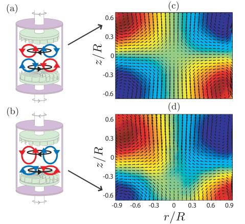
Figure 2: (a) and (b) Schematic drawings of the flow topology and (c) and (d) corresponding experimental maps of mean velocity field of the turbulent von Kármán flow at $Re=800\,000$ for (c) $\theta=0$ ($\overline{I}=0$) and (d) $\theta=-0.0147$ ($\overline{I}<0$). The color maps the azimuthal velocity $u_{\varphi}$, from blue to red (“jet” colormap), whereas the arrows map the $(u_{r},u_{z})$ field. The resolution has been reduced by a factor 2 for better visibility. The $r\leftrightarrow-r$ symmetry in (c) and (d) reveals that the time-averaged mean fields are axisymmetric.

When $\theta=0$, the experimental system is symmetric with respect to any $\cal{R}_{\pi}$-rotation exchanging the two impellers: the problem conditions are invariant under $\pi$-rotation around any radial axis passing through the center of the cylinder (Fig. 1). The symmetry group for such experimental system is $O(2)$ nore2003 . When $\theta\neq 0$, the experimental system is no more $\cal{R}_{\pi}$-symmetric, the symmetry switching to the $SO(2)$ group of rotations. However, the parameter $\theta$, when small but non-zero, can be considered as a measure of the distance to the exact $O(2)$ symmetry: the stricto sensu $SO(2)$ system at small $\theta$ can be considered as a slightly broken $O(2)$ system chossat93 ; porter2005 . Depending on the value of $\theta$, the flow can respond by displaying different symmetries: (i) the exact $\cal{R}_{\pi}$-symmetric flow composed of two toric recirculation cells separated by an azimuthal shear layer located at $z=0$ when $\theta=0$ (Figs. 2(a) and (c)); (ii) an asymmetric two-cells flow, the shear layer being closer to the slowest impeller ($z\neq 0$), when $\theta\neq 0$ (Figs. 2(b) and (d)); (iii) and finally, a fully non symmetric one-cell flow, the whole shear layer being concentrated in between the blades of the slowest impeller, when $\theta$ becomes large enough ravelet2004 ; ravelet2008 ; cortet09 .

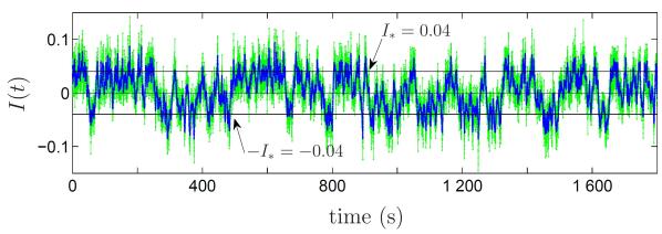
Figure 3: Global angular momentum $I(t)$ as a function of time for an experiment performed at $Re=43\,000$ for $\theta=0$. Green/light gray dots are PIV data sampled at 15 Hz and blue/dark gray dots correspond to 1 Hz low-pass filtered data $I_{f}(t)$. Eye-guiding lines have been drawn at $I(t)=\pm I_{*}=\pm 0.04$.

In order to quantify the distance of the flow to the $\cal{R}_{\pi}$-symmetry, we use the normalized and space-averaged angular momentum $I(Re,\theta,t)$ as order parameter:

$$I(t)=\frac{1}{\cal{V}}\int_{\cal{V}}rdrd\varphi dz\,\frac{ru_{\varphi}(t)}{\pi\,R^{2}\,(f_{1}+f_{2})}$$

where $\cal{V}$ is the volume of the flow note1 . An example of time variation of $I(t)$ at $\theta=0$ in the turbulent regime is provided in Fig. 3. We assume that ergodicity holds, meaning that the instantaneous turbulent flow is exploring in time its energy landscape according to its statistical probability. In this framework, the time average value $\overline{I}$ of $I(t)$ is equivalent to a statistical mechanics ensemble average providing the average is performed over a long enough duration in order to correctly sample the slowest time-scales. Then, using this ensemble averaged order parameter, we define a susceptibility of the flow to symmetry breaking $\chi_{I}$ as:

$$\chi_{I}=\left.\frac{\partial\overline{I}}{\partial\theta}\right|_{\theta=0},$$

Note that $\overline{I}$ is proportional to the mean altitude $z_{s}$ of the shear layer which is the natural measure of the flow symmetry. Contrary to $z_{s}$, $I(t)$ is defined for any instantaneous velocity field, including turbulent ones.

In the non-fluctuating laminar case, when $\theta=0$, $\overline{I}=0$ due to the symmetry of the flow. In contrast, as $\theta$ drifts away from $0$, the value of the angular momentum $\overline{I}$ becomes more and more remote from zero as the asymmetry of the flow grows. In such a framework, there is a formal analogy between ferromagnetic and turbulent systems. For ferromagnetism (resp. turbulence), the order parameter is the magnetization $M(T,h)$ (resp. the angular momentum $I(Re,\theta)$); the symmetry breaking parameter is the external applied field $h$ (resp. the relative driving asymmetry $\theta$); the control parameter is the temperature $T$ (resp. the Reynolds number $Re$, or a function of it).

In the sequel, we first investigate the influence of turbulence on $\overline{I}$ and $\chi_{I}$ as $Re$ increases from $150$ to $10^{6}$. In the laminar flow at $Re=150$, the symmetry parameter $\overline{I}=I(t)$ evolves linearly with $\theta$ (Fig. 4(c)) and the susceptibility is $\chi_{I}=0.240\pm 0.005$. Increasing the Reynolds number, one expects to reach fully developed turbulence around $Re=10\,000$ ravelet2008 . In such turbulent regimes, velocity fields of von Kármán flows are characterized by a high level of intrinsic fluctuations, i.e. fluctuations of the same order of magnitude than the mean values cortet09 . Therefore, even when $\theta=0$, the $\cal{R}_{\pi}$-symmetry is of course broken for the instantaneous flow. However, as usually observed for classical turbulence, this symmetry is restored for the time-averaged flow (Fig. 2(c)), which proves that time averages are long enough to correctly sample the slowest flow time scales. Then, as in the case of the laminar flow, when $\theta$ is varied, we observe the breaking of the $\cal{R}_{\pi}$-symmetry of the mean flow (Fig. 2(d)).

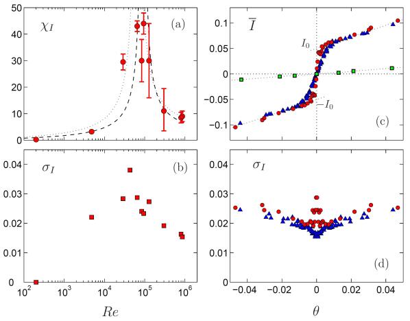
Figure 4: Reynolds number dependence of: (a) Susceptibility to symmetry-breaking $\chi_{I}$ of the von Kármán mean flow at $\theta=0$ and (b) standard deviation $\sigma_{I}$ of the global angular momentum $I(t)$ at $\theta=0$. In (a), the dotted line corresponds to the mean field theory approach with a critical Reynolds number $Re_{\chi}=70\,000$ and the dashed line to $Re_{\chi}=90\,000$; (c) global angular momentum $\overline{I}$ and (d) standard deviation $\sigma_{I}$ as a function of $\theta$ for $Re=150$ (green $\Box$), $Re=65\,000$ (red $\circ$) and $Re=800\,000$ (blue $\triangle$). In (a) and (b), horizontal error bars are of the order of the marker size. In (a) vertical error bars are computed as the maximum error that can arise from the sharp dependence of $\sigma_{I}$ with $\theta$ around $\theta=0$.

In Fig. 4(c), we see that, at $Re=800\,000$, in the close vicinity of $\theta=0$, $\overline{I}(\theta)$ evolves actually much more rapidly with $\theta$ than in the laminar case with the susceptibility being larger by more than one order of magnitude: $\chi_{I}=9\pm 1$. Therefore, turbulence seems to enhance dramatically the sensitivity of the flow to symmetry breaking. Furthermore, for intermediate $Re=65\,000$, the slope of $\overline{I}(\theta)$ around $\theta=0$ is even much steeper —$\chi_{I}=43\pm 1$— than for $Re=800\,000$. In Fig. 4(a), we plot the susceptibility with respect to $Re$. We see that the susceptibility actually grows by more than two orders of magnitude —from $0.24$ to $46$— between $Re=150$ and $Re\simeq 90\,000$, before decreasing by a factor 4 between $Re\simeq 90\,000$ and $Re=800\,000$. These results suggest a critical behaviour for $\chi_{I}(Re)$ near $Re=Re_{\chi}=90\,000\pm 10\,000$: a divergence —revealing a continuous second order phase transition— or only a maximum —revealing either a subcritical bifurcation or a continuous transition with finite-size effect. This cannot be experimentally tested further since the highest measured $\chi_{I}$ are already of the order of the highest measurable value considering the $\theta$ precision of our setup. For higher $|\theta|$, we observe a crossover —for the slope— in the curve $\overline{I}(\theta)$ at $|\theta_{r}|=(6\pm 1)\times 10^{-3}$ for $Re=800\,000$ and very close to $\theta=0$, at $|\theta_{r}|=(0.9\pm 0.15)\times 10^{-3}$, for $Re=65\,000$ (Fig. 4(c)). For $|\theta|>|\theta_{r}|$, we recover the laminar slow evolution of $\overline{I}$ with $\theta$ up to $\theta=\pm 0.1$ where the flow bifurcates to the one-cell topology (not shown). Since $\overline{I}(\theta)$ is quite independent of $Re$ for $|\theta|>|\theta_{r}|$ at large $Re$, we can extrapolate this linear behaviour to $\theta=0$. This extrapolation describes the ideal behaviour at critical Reynolds number $Re_{\chi}$ if $\chi_{I}$ diverges: a jump of $\overline{I}$ between $-I_{0}$ and $+I_{0}$ where $I_{0}\simeq 0.05$. This can be interpreted as a spontaneous “turbulent momentization” $I_{0}$ at $\theta=0$ —possibly affected by finite-size effects— by analogy with the spontaneous magnetization $M_{0}$ at zero external field for ferromagnetism. It is also similar to the experimental results of Torre2007 .

A signature of this momentization can be seen on the instantaneous global angular momentum $I(t)$ for $Re$ near the peak of susceptibility and $\theta=0$ (e.g. in Fig. 3). Indeed, one observes that $I(t)$ does not remain near zero (its mean value) but shows a tendency to lock preferentially on the plateaus $\pm I_{*}$ with $I_{*}=0.04\simeq I_{0}$. Therefore, the turbulent flow explores a continuum of metastable symmetry breaking patterns evidenced by $-0.04\lesssim I_{f}(t)\lesssim 0.04$, $I_{f}(t)$ being the 1 Hz low-pass filtered value of $I(t)$. The global angular momentum actually fluctuates very much along time with two separate time scales: fast fluctuations related to “traditional” small scale turbulence and time intermittencies corresponding to residence time of few tens of seconds. If one performs a time average over one of these intermittent periods only, one obtains a time localized “mean” flow, which breaks spontaneously the symmetry, analogous to what is obtained for true mean flows when $\theta\neq 0$ as presented in Figs. 2(b) and (d).

The presence of strong fluctuations is not surprising here: close to a phase transition we expect critical fluctuations. To check this, we compute the standard deviation $\sigma_{I}(Re,\theta)$. Fig. 4(b) shows, for $\theta=0$, how $\sigma_{I}$ varies from zero in laminar case to finite values for highly turbulent flows going through a maximum at Reynolds number $Re=Re_{\sigma}=45\,000\pm 10\,000$ located below the peak of susceptibility at $Re_{\chi}$. Additionally, in Fig. 4(d), the dependence of $\sigma_{I}$ as a function of the symmetry control parameter $\theta$ reveals a strong difference between the two Reynolds numbers shown: $\sigma_{I}(\theta)$ presents a sharp and narrow peak at $\theta=0$ for $Re=65\,000$, which does not exist for $Re=800\,000$. The amplitude of this peak from its bottom to its top actually measures the additional amount of low frequency symmetry fluctuations due to the multistability. This amount of fluctuations appears to be connected to the susceptibility increase below $Re_{\chi}$.

The previous experimental results set a strong connection between the spontaneous symmetry fluctuations of the flow and the mean flow response to the system symmetry breaking: the interpretation of the large fluctuations of $I(t)$ in terms of multistability suggests that the strong observed linear response of the mean flow (Fig. 4(c)) with respect to $\theta$ in the close vicinity of $\theta=0$ is the result of a temporal mixing between the metastable states in different proportions.

Nevertheless, as the Reynolds number is varied, two distinct maxima have been evidenced in our turbulent flow: one for the susceptibility $\chi_{I}$ to the $O(2)$-symmetry breaking near $Re=Re_{\chi}\simeq 90\,000$, and the other for the standard deviation of the global angular momentum $I(t)$ near $Re=Re_{\sigma}\simeq 45\,000$. In this Reynolds number range, the turbulence is generally expected to be fully developed, i.e. any non-dimensional characteristic quantity of the flow should be $Re$-independent. This is definitively not the case in this von Kármán experiment. Actually, visual observations of the flow reveal an increase of the average azimuthal number $m$ of large scale vortices in the shear-layer from $m=3$ to $m=4$ through an Eckhaus-type transition, between $Re_{\sigma}$ and $Re_{\chi}$. In the following, we make the hypothesis that at least one critical phenomenon exists in the range $50\,000\apprle Re\apprle 100\,000$. Using the turbulent von Kármán-ferromagnetism analogy, we can check how classical mean field predictions for second order phase transition apply to our system. In terms of susceptibilities, it predicts a critical divergence at a temperature $T_{c}$: $\chi\propto\left|T-T_{c}\right|^{-1}$. Since the logarithm of the Reynolds number has already been proposed as the control parameter governing the statistical temperature of turbulent flows —$T\sim 1/\log Re$ castaingbis — , this prediction translates in our case into:

$$\chi_{I}\propto\left|1/\log Re-1/\log Re_{c}\right|^{-1}.$$

This formula reasonably describes our data with $Re_{c}$ between typically $70\,000$ and $90\,000$ (Fig. 4(a)) supporting the asymmetry between the two branches even with a unique exponent $-1$. As far as fluctuations are concerned, it is difficult to find a reasonable critical exponent for $\sigma_{I}$. However, the results show that the maxima for $\chi_{I}$ and $\sigma_{I}$ are clearly separated. This is at variance with classical phase transition theory, stating e.g. in the Fluctuation Dissipation Theorem that $\sigma_{I}^{2}$ should be proportional to $\chi_{I}$. A reason for this discrepancy lies in the high level of intrinsic fluctuations in our system that makes this transition non-classical. Instabilities or bifurcations occurring on highly fluctuating systems are commonly found in natural systems and the literature reports transitions and symmetry breaking at high Reynolds number (see, e.g., references mujica ; gibert2009 ; castaing ; lohse2009 ; Torre2007 ; tabeling96 ; tabeling02 ; dynamoP1 ; dynamoP5 ; ravelet2004 ; ravelet2008 ) but the corresponding theoretical tools are still today not well settled. Existing studies of phase transitions in the presence of fluctuations generally considers systems in which an external noise —additive or multiplicative— is introduced review_noise . In particular, it has been shown in models that multiplicative noise can produce an ordered symmetry breaking state through a non equilibrium phase transition vandenbroeck94 . This behaviour could be at the origin of our observed transition. Finally, we can notice that, as the Reynolds number increases, the “turbulent momentization”$I_{0}$ first increases and then decreases, contrary to the magnetization in the usual para-ferromagnetic transition. This result is reminiscent of a reentrant noise-induced phase transition similar to that observed in the annealed Ising model thorpe76 ; genovese98 . The study of the evolution of $I_{0}$ and/or $I_{*}$ with $Re$ requires more statistics and is left for future work. Finally, our turbulent system, in which we can have access both to the spatiotemporal evolution of the states and to the mean thermodynamic variables, appears as a a unique tool to study out-of-equilibrium phase transitions in strongly fluctuating systems.

- (1) L. D. Landau and E. M. Lifchitz, Statisticheskaya Fisika (Nauka, Moscow, 1976).
- (2) P. Manneville, Dissipative Structures and Weak Turbulence (Academic Press, Boston, 1990).
- (3) U. Frisch, Turbulence - The Legacy of A N Kolmogorov (Cambridge University Press, Cambridge, 1995).
- (4) B. Hof, J. Westerweel, T. Schneider and B. Eckhardt, Nature 443, 59 (2006).
- (5) P. Tabeling et al., Phys. Rev. E 53, 1613 (1996).
- (6) P. Tabeling and H. Willaime, Phys. Rev. E 65, 066301 (2002).
- (7) F. Ravelet, L. Marié, A. Chiffaudel and F. Daviaud, Phys. Rev. Lett. 93, 164501 (2004).
- (8) F. Chillá, M. Rastello, S. Chaumat and B. Castaing, Eur. Phys. J. B 40, 223 (2004).
- (9) N. Mujica and D. P. Lathrop, J. Fluid Mech. 551, 49 (2006).
- (10) F. Ravelet, A. Chiffaudel and F. Daviaud, J. Fluid. Mech. 601, 339 (2008).
- (11) R. Stevens et al., Phys. Rev. Lett. 103, 024503 (2009).
- (12) C. Nore, L. S. Tuckerman, O. Daube and S. Xin, J. Fluid Mech. 477, 1 (2003).
- (13) P. Chossat, Nonlinearity 6, 723 (1993).
- (14) J. Porter and E. Knobloch, Physica D 201, 318 (2005).
- (15) P.-P. Cortet et al., Phys. Fluids 21, 025104 (2009).
- (16) A. de la Torre and J. Burguete, Phys. Rev. Lett. 99, 054101 (2007); J. Burguete and A. de la Torre, Int. J. Bif. and Chaos 19, 2695 (2009).
- (17) B. Castaing, J. Phys. II 6, 105 (1996).
- (18) M. Gibert et al., Phys. Fluids 21, 035109 (2009).
- (19) R. Monchaux et al., Phys. Rev. Lett. 98, 044502 (2007).
- (20) R. Monchaux et al., Phys. Fluids 21, 035108 (2009).
- (21) N. G. van Kampen, Stochastic Processes in Physics and Chemistry (North-Holland Personal Library, Elsevier, Amsterdam, 1981).
- (22) C. Van den Broeck, J. Parrondo and R. Toral, Phys. Rev. Lett. 73, 3395 (1994).
- (23) M. Thorpe and D. Beeman, Phys. Rev. B 14, 188 (1976).
- (24) W. Genovese, M. Munoz and P. Garrido, Phys. Rev. E 58, 6828 (1998).
- (25) Practically, is computed from PIV-data restricted to a meridian plane only but, since azimuthal flow fluctuations are strong, time-average over several rotation periods —statistically equivalent to spatial azimuthal averaging— estimate correctly the 3D-value of (see details in Ref. cortet09 ).