Effects of uncertainties and errors on Lyapunov control

Abstract

Lyapunov control (open-loop) is often confronted with uncertainties and errors in practical applications. In this paper, we analyze the robustness of Lyapunov control against the uncertainties and errors in quantum control systems. The analysis is carried out through examinations of uncertainties and errors, calculations of the control fidelity under influences of the certainties and errors, as well as discussions on the caused effects. Two examples, a closed control system and an open control system, are presented to illustrate the general formulism.

I introduction

Quantum control is the manipulation of the temporal evolution of a system in order to obtain a desired target state or value of a certain physical observable, realizing it is a fundamental challenge in many fields dong09 ; wiseman10 ; rabitz09 , including atomic physics chu02 , molecular chemistry rabitz00 and quantum information nielsen00 . Several strategies of quantum control have been introduced and developed from classical control theory. For example, optimal control theory has been used to assist in control design for molecular systems and spin systems khaneja01 ; alessandro01 . A learning control method has been presented for guiding the control of chemical reactions rabitz00 . Quantum feedback control approaches including measurement-based feedback and coherent feedback have been used to improve performance for several classes of tasks such as preparing quantum states, quantum error correction and controlling quantum entanglement wiseman93 ; doherty00 . Robust control tools have been introduced to enhance the robustness of quantum feedback networks and linear quantum stochastic systems helon06 ; james08 .

Control systems are broadly classified as either closed-loop or open-loop. An open-loop control system is controlled directly, and only, by an input signal, whereas a closed-loop control system is one in which an input forcing function is determined in part by the system response. Among the open-loop controls, Lyapunov control has been proven to be a sufficient control to be analyzed rigourously, moreover, this control can be shown to be highly effective for systems that satisfy certain sufficient conditions that roughly speaking are equivalent to the controllability of the linearized system.

Lyapunov control for quantum systems in fact use a feedback design to construct an open-loop control. In other words, Lyapunov control is used to first design a feedback law which is then used to find the open-loop control by simulating the closed-loop system. Then the control is applied to the quantum system in an open-loop way. From the above description of Lyapunov control, we find that the Lyapunov control includes two steps: (1) for any initial states and a system Hamiltonian (assumed to be known exactly), design a control law, i.e., calculate the control field by simulating the dynamics of the closed-loop system, (2) apply the control law to the control system in an open-loop way. Although some progress has been made, more research effort is necessary in Lyapunov control, especially, the robustness of quantum control systems has been recognized as a key issue in developing practical quantum technology. In this paper, we study the effect of uncertainties and errors on the performance of Lyapunov control. The uncertainties come from initial states and system Hamiltonian, and errors may occur in applying the control field (control law). Through this study, we show the robustness of Lyapunov control against uncertainties and errors. In particular, the relation between the uncertainties and the fidelity is established for a closed two-level control system and an open four-level control system.

This paper is organized as follows. In Sec.II, we introduce the Lyapunov control and formulate the problem. A general formulism is given to examine the robustness of the Lyapunov control. In Sec. III, we exemplify the general formulation in Sec.II through a closed and an open quantum control systems. Concluding remarks are given in Sec. IV.

II problem formulation

A control quantum system can be modeled in different ways, either as a closed system evolving unitarily governed by a Hamiltonian, or as an open system governed by a master equation. In this paper, we restrict our discussion to a $N$-dimensional open quantum system, and consider its dynamics as Markovian. The discussion is applicable for closed systems, since closed system is a special case of open system with zero decoherence rates. Therefore we here consider a system that obeys the Markovian master equation ($\hbar=1,$ throughout this paper),

$$\dot{\rho}=-i[H,\rho]+{\mathcal{L}}(\rho)$$ (1)

with

$${\mathcal{L}}(\rho)=\frac{1}{2}\sum_{m=1}^{M}\lambda_{m}([J_{m},\rho J_{m}^{\dagger}]+[J_{m}\rho,J_{m}^{\dagger}]),$$

and

$$H=H_{0}+\sum_{n=1}^{F}f_{n}(t)H_{n},$$

where $\lambda_{m}\ (m=1,2,...,M)$ are positive and time-independent parameters, which characterize the decoherence and are called decoherence rates. Furthermore, $J_{m}\ (m=1,2,...,M)$ are the Lindblad operators, $H_{0}$ is the free Hamiltonian and $H_{n}\ (n=1,2,...,F)$ are control Hamiltonians, while $f_{n}(t)\ (n=1,2,...,F)$ are control fields. Equation (1) is of Lindblad form, this means that the solution to Eq. (1) has all the required properties of physical density matrix at any times. Since the free Hamiltonian can usually not be turned off, we take nonstationary states $\rho_{D}(t)$ as target states that satisfy,

$$\dot{\rho}_{D}(t)=-i[H_{0},\rho_{D}(t)].$$ (2)

The control fields $\{f_{n}(t),\ n=1,2,3,...\}$ can be established by Lyapunov function. Define $V(\rho_{D},\rho)$,

$$V(\rho_{D},\rho)=\mbox{Tr}(\rho_{D}^{2})-\mbox{Tr}(\rho\rho_{D}),$$ (3)

we find $V\geq 0$ and

$$\dot{V}=-\sum_{n}^{F}f_{n}(t)\mbox{Tr}\{\rho_{D}[-iH_{n},\rho]\}-\mbox{Tr}[\rho_{D}\mathcal{L}(\rho)].$$ (4)

For $V$ to be a Lyapunov function, it requires $\dot{V}\leq 0$ and $V\geq 0.$ If we choose a $n_{0}$ such that $f_{n_{0}}(t)\mbox{Tr}\{\rho_{D}[-iH_{n_{0}},\rho]\}+\mbox{Tr}[\rho_{D}\mathcal{L}(\rho)]=0$, and $f_{n}(t)=\mbox{Tr}\{\rho_{D}[-iH_{n},\rho]\}$ for $n\neq n_{0}$, then $\dot{V}\leq 0.$ With these choices, $V$ is a Lyapunov function. Therefore, the evolution of the open system with Lyapunov control governed by the following nonlinear equationsyi09

$$\dot{\rho}(t) = -i[H_{0}+\sum_{n}f_{n}(t)H_{n},\rho(t)]+\mathcal{L}(\rho),$$

$$f_{n}(t) = \mbox{Tr}\{[-iH_{n},\rho]\rho_{D}\},\mbox{ for }n\neq n_{0},$$

$$f_{n_{0}}(t) = -\frac{\mbox{Tr}[\rho_{D}\mathcal{L}(\rho)]}{\mbox{Tr}\{\rho_{D}[\rho,iH_{n_{0}}]\}},\mbox{and}$$

$$\dot{\rho}_{D}(t) = -i[H_{0},\rho_{D}(t)]$$ (5)

is stable in Lyapunov sense at least. In Eqs (2) and (3), we have identified $\rho_{D}(t)$ with target states, this means that if a quantum system is driven into the target states, it will be maintained in these states under the action of the free Hamiltonian. However, in practical applications, it is inevitable that there exist errors and uncertainties in the free Hamiltonian, in the initial states and in the control fields. These uncertainties and errors would disturb the dynamics and steer the system away from the target state. In the following, we suppose that the uncertainties can be approximately described as perturbations $\delta H_{0}$ in the free Hamiltonian, and as deviations $\delta\rho_{0}$ in the initial state as well as fluctuations $\delta f_{n}\ (n$ may take $1,2,3,...)$ in the control fields. Then the actual final state $\rho_{R}(t)$ of the control system starting from $(\rho_{0}+\delta\rho_{0})$ governed by Eq. (5) with $(H_{0}+\delta H_{0})$ and $[f_{n}(t)+\delta f_{n}(t)]$ instead of $H_{0}$ and $f_{n}(t)$ would be different from $\rho_{D}(t).$ We quantify the difference between the target states $\rho_{D}(t)$ and the practical states $\rho_{R}(t)$ by using the fidelity defined by $F(\rho_{D},\rho_{R})=\text{Tr}\sqrt{\rho_{D}^{\frac{1}{2}}\rho_{R}\rho_{D}^{\frac{1}{2}}}.$

For a Lyapunov control with negative gradient of Lyapunov function in the neighborhood of target states, the controlled system state will be attracted to and maintained in the target state, when there are no uncertainties and errors. With uncertainties and errors, the problem of robustness of the control system is not trivial, because the Lyapunov-based feedback design for the control law would induce nonlinearity in the control system. The LaSalle invariant principlelasalle61 tells that the autonomous dynamical system Eq.(5) converges to an invariant set defined by $\mathcal{E}=\{\rho_{in}:\dot{V}=0\}$, which is equivalent to $f_{n}(t)=0,\ n=1,2,3,...$ by Eq.(5). This set is in general not empty and the final state will be in it. From Eqs. (4) and (5) we find that the invariant set is an intersection of all sets $\mathcal{E}_{n}$ $(n=1,2,3,...,n\neq n_{0})$, each satisfies,

$$\mathcal{E}_{n}=\{\rho_{in,n}:\text{Tr}(\rho_{d}H_{n}\rho_{in,n}-H_{n}\rho_{d}\rho_{in,n})=0\},\ \ n\neq n_{0}.$$ (6)

Since the control fields are proportional to $\dot{V}$, the errors in the control fields would change the invariant set. The uncertainties in the initial state affect the invariant set in the same way, and the uncertainties in the free Hamiltonian change the target sets $\rho_{d}(t)$, leading to an invariant set different from that without uncertainties. In the next section, we will illustrate and exemplify the effect of errors and uncertainties on the fidelity through simple examples.

III illustration

In this section, we first introduce a Lyapunov control on a closed two-level quantum system, then we study the robustness of this Lyapunov control by examining the effects of uncertainties and errors on the fidelity of control. Next, we extend this study into open systems by considering a dissipative four-level system and steering it to a target state in its decoherence-free subspace (DFS).

We start with a closed two-level system described by the Hamiltonian,

$$H=\frac{\omega}{2}\sigma_{z}+f(t)\sigma_{x}\equiv H_{0}+H_{1},$$ (7)

where $H_{0}=\frac{\omega}{2}\sigma_{z}$ denotes the free Hamiltonian of the system, $H_{1}=f(t)\sigma_{x}$ is the control Hamiltonian with a control field $f(t).$ We define one of the eigenstates of $H_{0}$, say the ground state $|g\rangle$, as the target state, the Lyapunov function in Eq. (3) for this closed system is then

$$V(|g\rangle,|\Phi(t)\rangle)=1-|\langle g|\Phi(t)\rangle|^{2}.$$ (8)

For closed system, the Liouvillian ${\mathcal{L}}(\rho)$ vanishes, thus we do not need to choose a control field $f_{n_{0}}(t)$ in Eq. (5) to cancel the drift term. The only control field $f(t)$ that can be derived from Eq. (5) is,

$$f(t)=2{\mbox{Im}}(\langle g|\sigma_{x}|\Phi(t)\rangle\langle\Phi(t)|g\rangle).$$ (9)

Here $|\Phi(t)\rangle$ represents states at time $t$ starting from an initial states

$$|\Phi(0)\rangle=\cos\beta_{0}|e\rangle+\sin\beta_{0}e^{i\phi_{0}}|g\rangle,$$

under the action of the Hamiltonian $H$ without any uncertainties and errors. We further suppose that the uncertainties in the free Hamiltonian $H_{0}$ can be described as a perturbation,

$$\delta H_{0}=\delta_{x}\sigma_{x}+\delta_{z}\sigma_{z},$$ (10)

and the uncertainties in the initial state $|\Phi(0)\rangle$ can be characterized by replacing $\beta_{0}$ and $\phi_{0}$ with $(\beta_{0}+\delta\beta_{0})$ and $(\phi_{0}+\delta\phi_{0})$, respectively.

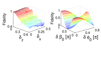
Figure 1: (Color online) Fidelity of Lyapunov control versus the uncertainties in the free Hamiltonian (left) and in the initial states (right). $\omega=4$ (in arbitrary units) and $\phi_{0}=\beta_{0}=\frac{\pi}{4}$ are chosen for this plot.

We describe the errors in the control fields $f(t)$ as fluctuations $\delta(t)\cdot f(t)$ with random number $\delta(t)$. With these descriptions, the practical control system can be described by,

$$i\hbar\frac{\partial}{\partial t}|\psi(t)\rangle_{R}=[H_{0}+\delta H_{0}+f(t)H_{1}(1+\delta(t))]|\psi(t)\rangle_{R},$$ (11)

with initial condition $|\Phi(0)+\delta\Phi(0)\rangle=\cos(\beta_{0}+\delta\beta_{0})|e\rangle+\sin(\beta_{0}+\delta\beta_{0})e^{i(\phi_{0}+\delta\phi_{0})}|g\rangle.$

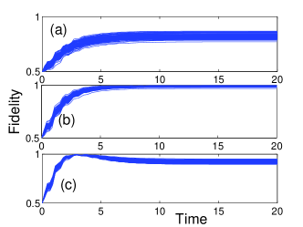
Figure 2: (Color online) Fidelity of Lyapunov control as a function of time. This plot shows the effects of fluctuations in the control field $f(t)$ on the fidelity. (a), (b) and (c) are for different types of fluctuations. (a) The fluctuation $\delta(t)$ was taken from $(-1)$ to zero; (b) from $(-1)$ to (+1); and (c) from 0 to (+1). All fluctuations are taken randomly. The other parameters chosen are the same as in Fig. 1. There are no uncertainties in the free Hamiltonian and in the initial states.

We have performed numerical simulations for Eq. (11), selected results are presented in figures 1 and 2. Figure 1 shows the control fidelity as a function of uncertainties $(\delta_{x},\delta_{y})$ in the free Hamiltonian and uncertainties $(\delta\beta_{0},\delta\phi_{0})$ in the initial state. Two observations can be made from the figures. (1) The control fidelity rapidly depends on the uncertainties $\delta_{z}\sigma_{z}$, whereas it is not sensitive to $\delta_{x}\sigma_{x}$, (2) the control fidelity is an oscillating function of $\delta\beta_{0}$ and $\delta\phi_{0}$ with different periods. These observations indicate that the Lyapunov control on closed systems is robust against the uncertainties that commute with the control Hamiltonian, while it is fragile with the other uncertainties in the free Hamiltonian. This claim is confirmed by Fig. 2, where the effect of fluctuations in the control field on the control fidelity is shown. One can clearly see from figure 2 that there are almost no effects for the fluctuations with zero mean on the fidelity. This can be understood as follows. Since the fluctuations is randomly chosen for the control fields, the net effect intrinsically equals to an average over all fluctuations, which must be zero for fluctuation with zero mean.

Now we turn to another example that shows the robustness of Lyapunov control on open quantum systems. We borrow the model in Ref.yi10 shown in Fig.3, where a four-level system coupling to two external lasers and being subject to decoherence has been considered. The Hamiltonian of this system has the form,

$$H_{0}=\sum_{j=0}^{2}\Delta_{j}|j\rangle\langle j|+(\sum_{j=1}^{2}\Omega_{j}|0\rangle\langle j|+h.c.),$$ (12)

where $\Omega_{j}\ \ (j=1,2)$ are coupling constants. Without loss of generality, in the following the coupling constants are parameterized as $\Omega_{1}=\Omega\cos\phi$ and $\Omega_{2}=\Omega\sin\phi$ with $\Omega=\sqrt{\Omega_{1}^{2}+\Omega_{2}^{2}}.$ The excited state $|0\rangle$ is not stable, it decays to the three stable states with rates $\gamma_{1}$, $\gamma_{2}$ and $\gamma_{3}$ respectively. We assume this process is Markovian and can be described by the Liouvillian,

$$\mathcal{L}(\rho)=\sum_{j=1}^{3}\gamma_{j}(\sigma_{j}^{-}\rho\sigma_{j}^{+}-\frac{1}{2}\sigma_{j}^{+}\sigma_{j}^{-}\rho-\frac{1}{2}\rho\sigma_{j}^{+}\sigma_{j}^{-})$$ (13)

with $\sigma_{j}^{-}=|0\rangle\langle j|$ and $\sigma_{j}^{+}=(\sigma_{j}^{-})^{\dagger}.$ It is not difficult to find that the two degenerate eigenstates $|D_{1}\rangle=\cos\phi|2\rangle-\sin\phi|1\rangle,$ $|D_{2}\rangle=|3\rangle,$ of the free Hamiltonian $H_{0}$ form a DFS. Now we show how to control the system to a desired target state (e.g., $|D_{1}\rangle$) in the DFS. For this purpose, we choose the control Hamiltonian

$$H_{c}=\sum_{j=1}^{3}f_{j}(t)H_{j}$$ (14)

with $H_{1}$ is a 4 by 4 matrix with all elements equal to 1. $H_{2}=|D_{1}\rangle\langle D_{2}|+|D_{2}\rangle\langle D_{1}|,H_{3}=|0\rangle\langle D_{2}|+|D_{2}\rangle\langle 0|.$ We shall use Eq. (5) to determine the control fields $\{f_{n}(t)\}$, and choose

$$|\Psi(0)\rangle = \sin\beta_{1}\cos\beta_{3}|0\rangle+\cos\beta_{1}\cos\beta_{2}|1\rangle$$ (15)

$$+ \cos\beta_{1}\sin\beta_{2}|2\rangle+\sin\beta_{1}\sin\beta_{3}|3\rangle$$

as initial states for the numerical simulation, where $\beta_{1}$, $\beta_{2}$ and $\beta_{3}$ are allowed to change independently. The initial state written in Eq.(15) omits all (three) relative phases between the states $|0\rangle,|1\rangle,|2\rangle$ and $|3\rangle$ in the superposition, and satisfies the normalization condition. $f_{1}(t)$ here is specified to cancel the drift term $\text{Tr}[{\mathcal{L}}(\rho)\hat{A}]$ in $\dot{V},$ this means that $f_{1}(t)=-i\frac{\text{Tr}({\mathcal{L}}(\rho)\hat{A})}{\text{Tr}([\hat{A},H_{1}]\rho)},$ $f_{2}(t)$ and $f_{3}(t)$ are determined by Eq.(5).

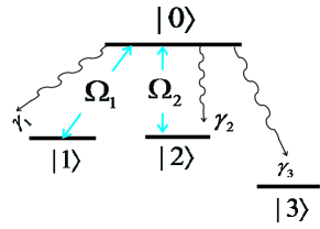
Figure 3: The schematic energy diagram. A four-level system with two degenerate stable states $|1\rangle$ and $|2\rangle$ in external laser fields. The two degenerate states are coupled to the excited state $|0\rangle$ by two separate lasers with coupling constants $\Omega_{1}$ and $\Omega_{2}$, respectively. While the stable state $|3\rangle$ is isolated from the other levels. The excited state $|0\rangle$ decays to $|j\rangle$ ($j=1,2,3$) with decay rate $\gamma_{j}$.

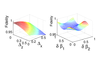
Figure 4: (Color online) The fidelity of control as a function of uncertainties in the free Hamiltonian (left) and in the initial state (right). The other parameters chosen are $\Omega=5,\phi=\frac{\pi}{5},\beta_{3}=\frac{\pi}{3},\beta_{1}=\frac{\pi}{5},\beta_{2}=\frac{\pi}{4},\gamma_{1}=\gamma_{2}=\gamma_{3}=\frac{1}{3}\gamma,\kappa_{2}=1,$ $\Delta_{0}=4,\Delta_{1}=\Delta_{2}=2$ and $\gamma=1.$ $\delta\beta_{1}$ and $\delta\beta_{2}$ are in unites of $\pi.$

We examine how the uncertainties in the free Hamiltonian and initial states as well as the errors in the control fields $f_{n}(t),(n=1,2,3,...)$ affect the fidelity of the control. These effects can be illustrated by numerical simulations on Eqs(12,13,14), with the free Hamiltonian $H_{0}$, the initial state $|\Phi(0)\rangle$ and the control fields $f_{n}(t)$ replaced by $(H_{0}+\delta H_{0})$, $|\Phi(0)+\delta\Phi(0)\rangle$ and $f_{n}(t)(1+\delta_{n})$, respectively. Here,

$$\delta H_{0}=\Delta_{x}(|0\rangle\langle 1|+|1\rangle\langle 0|)+\Delta_{z}(|0\rangle\langle 2|+|2\rangle\langle 0|),$$

(16)

$$|\Phi(0)+\delta\Phi(0)\rangle=\sin(\beta_{1}+\delta\beta_{1})\cos\beta_{3}|0\rangle$$

$$+\cos(\beta_{1}+\delta\beta_{1})\cos(\beta_{2}+\delta\beta_{2})|1\rangle$$

$$+\cos(\beta_{1}+\delta\beta_{1})\sin(\beta_{2}+\delta\beta_{2})|2\rangle$$

$$+\sin(\beta_{1}+\delta\beta_{1})\sin\beta_{3}|3\rangle,$$

and $\delta_{n}$ are random numbers ranging from $-1$ to $+1$. The fidelity versus the uncertainties (characterized by $\Delta_{x},\Delta_{z}$, $\delta\beta_{1},\delta\beta_{2}$) and errors ($\delta_{n},n=1,2,3,...)$ are presented in figures 4 and 5. Figures 4 and 5 tell us that the Lyapunov control on open system with the target state $|D_{1}\rangle$ is robust against the uncertainties in the initial state, and the fidelity is above $95\%$ when the uncertainties in the free Hamiltonian is bounded by 0.5 (in units of $\gamma$). The Lyapunov control is also robust gainst the fluctuations in the control fields $f_{n}(t)$ as figure 5 shows.

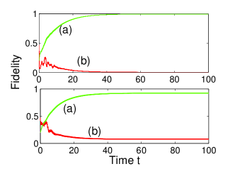
Figure 5: (Color online) Fidelity of Lyapunov control versus time $t$. The fluctuations $\delta_{n}\ (n=1,2,3,...)$ range from (-1) to (+1) for the upper panel, while from $(-1)$ to 0 (or 0 to (+1)) for the lower panel. (a) in both panels denotes the probability in state $|D_{1}\rangle$, while (b) in state $|D_{2}\rangle$. The other parameters chose are the same as in Fig. 4.

We note that the effects of fluctuations with zero mean are different from that with non-zero mean. This can understood as an average results taken over all fluctuations.

IV concluding remarks

To summarize, we have examined the robustness of Lyapunov control in quantum systems. The robustness is characterized by the fidelity of the quantum state to the target state. Uncertainties in the free Hamiltonian and in the initials states as well as the errors in the control fields diminish the fidelity of control. The relation between the uncertainties (errors) and the fidelity is established for a closed two-level control system and an open four-level control system. These results show that the Lyapunov control is robust against the type of uncertainties which commute with the control Hamiltonian, while it is fragile to the others. The fidelity is not sensitive to zero mean random fluctuations (white noise) in the control fields, but it really decreases due to the non-zero (positive or negative) mean fluctuations.

This work is supported by NSF of China under grant Nos 61078011 and 10935010, as well as the National Research Foundation and Ministry of Education, Singapore under academic research grant No. WBS: R-710-000-008-271.

References

- (1) D. Dong and I.R. Petersen, arXiv:0910.2350.
- (2) H.M. Wiseman and G.J. Milburn, Quantum Measurement and Control, Cambridge, England: Cambridge University Press, 2010.
- (3) H. Rabitz, New Journal of Physics 11, 105030 (2009).
- (4) S. Chu, Nature 416, 206 (2002).
- (5) H. Rabitz, R. de Vivie-Riedle, M. Motzkus and K. Kompa, Science 288, 824 (2000).
- (6) M.A. Nielsen and I.L. Chuang, Quantum Computation and Quantum Information, Cambridge, England: Cambridge University Press, 2000.
- (7) N. Khaneja, R. Brockett and S.J. Glaser, Phys. Rev. A 63,032308 (2001).
- (8) D. D Alessandro and M. Dahleh, IEEE Transactions on Automatic Control 46, 866 (2001).
- (9) H.M. Wiseman and G.J. Milburn, Phys. Rev. Lett. 70, 548 (1993).
- (10) A.C. Doherty, S. Habib, K. Jacobs K, H. Mabuchi and S.M. Tan, Phys. Rev. A 62, 012105 (2000).
- (11) C. D Helon and M.R. James, Phys. Rev. A 73, 053803 (2006).
- (12) M.R. James, H.I. Nurdin and I.R. Petersen, IEEE Transactions on Automatic Control 53,1787 (2008).
- (13) M.A. Pravia, N. Boulant, J. Emerson, E.M. Fortunato, T.F. Havel, D.G. Cory and A. Farid, Journal of Chemical Physics 119, 9993 (2003); L. Viola and E. Knill, Phys. Rev. Lett. 90, 037901 (2003); N. Yamamoto, and L. Bouten, IEEE Transactions on Automatic Control 54, 92 (2009).
- (14) J. LaSalle and S. Lefschetz, Stability by Lyapunov’s Direct Method with Applications (Academic Press, New York, 1961).
- (15) X. X. Yi, X. L. Huang, C. F. Wu, and C. H. Oh, Phys. Rev. A 80,052316(2009).
- (16) W. Wang, L. C. Wang, X. X. Yi, Phys. Rev. A 82, 034308 (2010).