A distinct peak-flux distribution of the third class of
gamma-ray bursts: A possible signature of X-ray flashes?

Abstract

Gamma-ray bursts are the most luminous events in the Universe. Going beyond the short-long classification scheme we work in the context of three burst populations with the third group of intermediate duration and softest spectrum. We are looking for physical properties which discriminate the intermediate duration bursts from the other two classes. We use maximum likelihood fits to establish group memberships in the duration-hardness plane. To confirm these results we also use k-means and hierarchical clustering. We use Monte-Carlo simulations to test the significance of the existence of the intermediate group and we find it with $99.8\%$ probability. The intermediate duration population has a significantly lower peak-flux (with $99.94\%$ significance). Also, long bursts with measured redshift have higher peak-fluxes (with $98.6\%$ significance) than long bursts without measured redshifts. As the third group is the softest, we argue that we have related them with X-ray flashes among the gamma-ray bursts. We give a new, probabilistic definition for this class of events.

1. Introduction

Gamma-ray bursts (GRBs) are the most powerful explosions known in the Universe (for a review see Mészáros (2006)). To discern the physical properties of GRBs as a whole, we need to understand the number of physically different underlying classes of the phenomenon (Zhang et al., 2009; Lü et al., 2010).

Before the launch of BATSE (Fishman et al., 1994), there were hints of two distinct populations (Mazets et al., 1981; Norris et al., 1984). The bimodality was established using BATSE observations of the duration by Kouveliotou et al. (1993). The subsequent classes were dubbed short and long type GRBs referring to their durations. More sophisticated statistical methods based on more data using one classification parameter (Horváth, 1998) and more than one observable property, showed three populations in the BATSE data (Mukherjee et al., 1998). These were further confirmed by subsequent analyses (Hakkila et al., 2003; Horváth et al., 2006; Chattopadhyay et al., 2007): the third population is intermediate in duration (Horváth, 2002).

Many statistical methods (e.g., maximum likelihood fitting, chi-square fitting, clustering) point to the presence of the third class with high significance. These methods reveal three groups in the data from different satellites (BATSE (Horváth et al., 2006), BeppoSAX (Horváth, 2009), RHESSI (Řípa et al., 2009), Swift (Horváth et al., 2008; Huja et al., 2009; Horváth et al., 2010)). These independent observations show that there is a good reason for the reality of the intermediate population.

While the existence of the intermediate population is proven with high significance using data from different experiments and using different statistical methods, a physical model to explain the origin of this third population is still missing (Mészáros, 2006).

With the launch of the Swift satellite (Gehrels et al., 2004), a new perspective has opened up of the study of gamma-ray bursts and their afterglows. The intermediate population in the studies so far has always been the softest among the groups, meaning intermediate GRBs emit the bulk of their energy in the low-energy gamma-rays. Swift’s gamma-ray detector BAT has an energy coverage from $15$ to $150$ keV - hence Swift is well suited for the study of the intermediate population.

Here we report on a significant difference in the peak-flux distribution between the intermediate and the short and between the intermediate and long populations. We identify a third population using a multi-component model and we show that this group has a significant overlap with X-ray flashes. We give a probabilistic definition of this class.

We present our sample in Section 2. In the next section we perform the classification with three methods and discuss the stability of the clustering. In Section 4. we present the peak-flux distribution of the classes. In Section 5. we analyze the samples with and without measured redshift. In Section 6. we interpret the findings and in Section 7. we conclude by summarizing the paper’s results.

2. Sample

The First Swift BAT Catalog (Sakamoto et al., 2008b) was augmented with bursts up to August 7, 2009 with measured $T_{90}$ and hardness ratio. After excluding the outliers and bursts without measured parameters, the sample consisting of the Sakamoto et al. (2008b) sample and our extension has a total of $408$ GRBs ($219$ from the Catalog and $189$ newer bursts).

Data reduction was carried out using HEAsoft version 6.3.3 and calibration database version 20070924. For light curves and spectra we ran the batgrbproduct pipeline. To obtain the spectral parameters we fitted the spectra integrated for the duration of the burst with a power law model and a power law model with an exponential cutoff. As in Sakamoto et al. (2008b) we have chosen the cutoff power law model if the $\chi^{2}$ of the fit improved by more than $6$.

The most widely used duration measure is $T_{90}$, which is defined as the period between the $5\%$ and $95\%$ of the incoming counts. To find the fluences ($S_{E_{min},E_{max}}$) we integrated the model spectrum in the usual Swift energy bands with $15-25-50-100-150$ keV as their boundaries. We define the hardness ratio ($H_{ij}$, where $i$ and $j$ mark the two energy intervals) as the ratio of the fluences in different channels for a given burst. For example $H_{32}=\frac{S_{50-100}}{S_{25-50}}$, where $S_{50-100}$ is the fluence of the burst for the entire duration measured in the $50-100$ keV range. Different hardness ratios are possible to define and we have used them to check our results.

Bursts have a wealth of measured parameters and it is possible to use many variations of them. The choice of $T_{90}$ has some draw-backs (Qin et al., 2010). It is not sensitive to quiescent episodes between the active phase of bursts (e.g., bursts with precursors). Also it cannot differentiate between bursts with an initial hard peak and a soft extended emission from bursts with constant long emission. In turn this latter type of burst with a hard initial spike and an extended soft emission can bias $H_{32}$ as well (Gehrels et al., 2006). Nevertheless, keeping in mind these draw-backs of $T_{90}$, this quantity is still one of the most important measures of GRBs, and hence its use is straightforward. This question is discussed also in Section 3.5.

3. Classification

3.1. The choice of variables

There are many indications that the phenomenon which we observe as gamma-ray bursts has more than one underlying population. The goal is to identify classes which are physically different. We choose the duration and the hardness ratio of bursts as the principal measure. This choice has been made by other studies as well (Dezalay et al., 1996; Horváth et al., 2006).

The choice of variables for the clustering deserves some justification. Satellites generally observe many properties and subsequent observations add to the volume of the parameters belonging to a burst. Bagoly et al. (1998) showed that two principal components are enough to describe the data in the BATSE Catalog satisfactorily. Horváth et al. (2006) followed these arguments and used the $H_{32}$ hardness and the $T_{90}$ duration to classify the bursts. By using $T_{90}$ and $H_{32}$ we include a basic temporal and spectral characteristic of the bursts.

The reality of any classification is hard to assess. A good way to make sure that the classification is robust and has some physical significance is to check the groups’ stability with respect to various classification methods. We carry out three types of classifications: model-based multivariate classification, k-means clustering and hierarchical clustering.

In the mathematical literature there is a wealth of classification schemes. We use the algorithms implemented in the R software. The clustering methods can be divided to parametric and non-parametric schemes. Parametric schemes postulate that the data follows a pre-defined model (in our case a superposition of multi-variate Gaussian distributions) and give a membership probability for each gamma-ray burst belonging to a given group. Thus each burst will have assigned $k$ number of membership probabilities, where $k$ is the number of multivariate components (groups). This is called a fuzzy clustering (Yang, 1993). The non-parametric tests (k-means and hierarchical clustering), on the contrary, assign definitive memberships to each burst. However, here one needs to define the distance or similarity measure between the cases.

3.2. Model based clustering

As discussed in Horváth et al. (2006), we can assume that the observed distribution of bursts on the duration-hardness plane is a superposition of two or more groups. The conditional probability density ($p(\log_{10}T_{90},\log_{10}H_{32}|l)$), together with the probability of a burst being from a given group ($p_{l}$) using the law of full probabilities:

$$p(\log_{10}T_{90},\log_{10}H_{32})=\sum_{l=1}^{k}p(\log_{10}T_{90},\log_{10}H_{32}|l)p_{l},$$ (1)

where $k$ is the number of groups.

Studies show that for example the distribution of the logarithm of the duration can be adequately described by a superposition of three Gaussians (Horváth, 1998). In this section we thus use the model based on bivariate Gaussian distributions. We suppose that the joint distribution of the parameters can be described as a superposition of Gaussians. Previously Horváth et al. (2006) carried out a similar analysis on the duration-hardness plane of the BATSE Catalog where data was fitted with bivariate Gaussians.

One bivariate Gaussian will have the following joint distribution function:

$$p(\log_{10}T_{90},\log_{10}H_{32}|l)=\frac{1}{2\pi\sigma_{\log_{10}T_{90}}\sigma_{\log_{10}H_{32}}\sqrt{1-r^{2}}}\exp\left(-\frac{1}{2(1-r^{2})}\left(\frac{(\log_{10}T_{90}-{\log_{10}T_{90}}_{C})^{2}}{\sigma_{\log_{10}T_{90}}^{2}}+\right.\right.$$

$$\left.\left.+\frac{(\log_{10}H_{32}-{\log_{10}H_{32}}_{C})^{2}}{\sigma_{\log_{10}H_{32}}^{2}}+\frac{2r(\log_{10}T_{90}-{\log_{10}T_{90}}_{C})(\log_{10}H_{32}-{\log_{10}H_{32}}_{C})}{\sigma_{\log_{10}T_{90}}\sigma_{\log_{10}H_{32}}}\right)\right),$$ (2)

where ${\log_{10}T_{90}}_{C}$ and ${\log_{10}H_{32}}_{C}$ are the ellipse center coordinates, $\sigma_{\log_{10}T_{90}}$ and $\sigma_{\log_{10}H_{32}}$ are the two standard deviations of the distribution and $r$ is the correlation coefficient.

Here we find the model parameters using the maximum likelihood method. The procedure is called Expectation-Maximization (EM). This consists of appointing a membership probability to each burst using an initial value of the parameters (E step). Then we calculate the parameters of the model using these memberships (M step). Using this new model we re-associate each burst to the groups and calculate the model parameters. We repeat these steps until the solution converge. It is proved that this procedure converges to the maximum likelihood solution of the parameters (Dempster et al., 1977).

3.3. Number of groups

It is important to decide on the true number of components to fit (the number of classes). In the model-based framework we have a better grip on this problem compared to the non-parametric methods. For our calculations we use the Mclust package (Fraley & Raftery, 2000) of R.

In the most general case the best model is found by maximizing the likelihood. It is possible to penalize a model for more degrees of freedom. A widely used version of this method is called the Bayesian Information Criterion (BIC) introduced by Schwarz (1978) (for astronomical applications see e.g. Liddle (2007)). The function to be maximized to get the best fitting model parameters has an additional term besides the log-likelihood:

$$BIC=2L_{max}-m\ln N,$$ (3)

where $L_{max}$(=$\ln l_{max}$) is the logarithm of the maximum likelihood of the model, $m$ is the number of free parameters, and $N$ is the size of the sample. This method takes into account the complexity of our model by penalizing for additional free parameters.

We use the BIC to find the most probable model (including the number of components) and the parameters of this model. In a two-dimensional fit the number of free parameters of a single bivariate Gaussian component is $6$ (two coordinates for the mean, two values of the standard deviations in different directions, a correlation coefficient and a weight). For $k$ bivariate Gaussians the number of free parameters is $6k-1$, since the sum of the weights is $1$.

In the most general model all $6$ parameters of each component can be varied. Some of the parameters may have interrelations between the components (e.g., all components have the same weight or shape, there is no correlation between the variables ($r=0$), etc.). In this way we construct models with less degrees of freedom. The possible interrelations between the parameters of the Gaussians are taken into account by trying different models with different types of constraints (for the list of models see the Mclust manual).

We have applied this classification scheme on our sample. We found that the model with three components gives the best fit for the data in the BIC sense, where the shape of the bivariate Gaussians is the same ($\sigma_{\log_{10}T_{90},i}=\sigma_{\log_{10}T_{90},j}$ and $\sigma_{\log_{10}H_{32},i}=\sigma_{\log_{10}H_{32},j}$ for $i,j=$ {short, long, intermediate}) for each group, only their weights are different with no correlation. This is called the EEI model in Mclust. The description of the model follows from its name: equal volume (E), equal shape (E) and the axes are parallel with the coordinate axes (I). In other words this is the model with optimal information content describing the data (see Fig. 1).

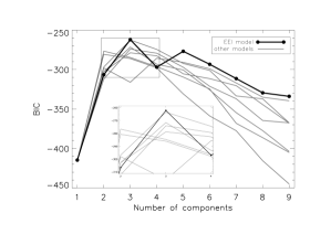
Figure 1.— Bayesian information criterion values for different models (different lines show different models) in function of the number of bivariate Gaussian components: the higher the value of the BIC, the more probable the model. The best model is marked in black and the highest value is reached for $k=3$. Also, some of the other models have their peak at $k=3$. The inset shows the magnified peak region.

We find that the best model has a value of $BIC=-262.14$. This model has three bivariate components. In the general case the maximum number of free parameters would thus be $m=17$. Taking into account the constraints of this model, the degrees of freedom here will be $m=10$ (three coordinate pairs for the center of the distributions, two standard deviations common for all three components and two weights).

The clustering method based on this model shows that a model containing three bivariate components is the most preferred. Models with two components have the best $BIC\sim-276$ and for models with four components the best $BIC\sim-274$, both are clearly below the maximum. In case of a maximum likelihood fit, we can infer the probability of the chance occurrence of a model compared to another. In this case the difference in the value of the BIC of two models informs us about the goodness of the model. According to Mukherjee et al. (1998) and references therein, differences in BIC in the $8$-$10$ range represent strong evidence in favor of the model with the higher BIC. In our case the differences are even bigger.

The best-fit model has $10$ free parameters and has three bivariate Gaussian components. The parameters of the model as well as the number of the bursts in the groups are in Table 1. The shortest and hardest group will be designated short, the longest and of moderate hardness will be called long and the intermediate duration group with the softest spectrum will be called intermediate. For the relation of the intermediate class to other studies on this topic see the discussion.

Table 1Bivariate model parameters for the best-fitted (EEI) model. The standard deviations in the direction of the coordinate axes and the correlation coefficients are constrained by the model.

Groups	$p_{l}$	${\lg T_{90}}_{C}$	${\lg H_{32}}_{C}$	$\sigma_{\lg T_{90}}$	$\sigma_{\lg H_{32}}$	$r$	$N_{l}$
short	$0.08$	$-0.331$	$0.247$	$0.509$	$0.090$	$0$	$31$
interm.	$0.12$	$1.136$	$-0.116$	$0.509$	$0.090$	$0$	$46$
long	$0.80$	$1.699$	$0.114$	$0.509$	$0.090$	$0$	$331$

To calculate the significance of three populations we carried out a Monte-Carlo simulation. We tested the hypothesis that the presence of the third population is only a statistical fluctuation. We generated $10000$ random catalogs, with the best $k=2$ model. We found that with the classification method only $0.2\%$ of the cases yielded a three component model while $99.8\%$ of cases produced a two component fit. This means that the probability that the third group is only a statistical fluctuation is $0.2\%$

To test the validity of the simulation , we have simulated again $10000$ samples of $408$ bursts, using the model parameters for the three population model in Table 1. We found that two populations are statistical fluctuation in $2.1\%$ of the cases compared to the three population model.

There is another three component model which has a very similar BIC value (the difference is only $\sim 1$, see the inset in Fig. 1). This model is called VEI and it has variable volume, meaning the product of the standard deviations is the same (V), equal shape (E) and the axes are parallel with the coordinate axes (I). It has $12$ degrees of freedom (three coordinate pairs for the centers of the distributions, three pairs of standard deviations with the restriction that their product is the same (four degrees of freedom) and two weights). Information Criterion gives only a weak hint as to which model is preferred. The VEI model gives a visibly different group structure. If we compare it to the three component EEI model the ratio of differently classified bursts is $26.7\%$. The group structure found by this model resembles the one found by Horváth et al. (2010) and will be addressed in the discussion section.

We assign class memberships using the ratio of the fitted bivariate models at the burst location on the duration-hardness plane. We call these membership probabilities. Any given burst is assigned to the group with the highest probability. Fuzzy classification (Yang, 1993) implies that we can define an indicator function in the following manner:

$$I_{\mathrm{l}}(\log_{10}T_{90},\log_{10}H_{32})=\frac{P_{\mathrm{l}}\times P(\log_{10}T_{90},\log_{10}H_{32}|l)}{\displaystyle\sum_{l\in\mathrm{\{short,interm.,long\}}}P_{\mathrm{l}}\times P(\log_{10}T_{90},\log_{10}H_{32}|l)}.$$ (4)

Here $P(\log_{10}T_{90},\log_{10}H_{32}|l)$ is the conditional probability density of a burst, assuming it comes from class $l$. $P_{l}$ is the probability of the $l$ class. The indicator function assigns a probability for a burst that it belongs to a given group.

In this framework there is no definite answer to the question: ”To which class does a specific burst belong?”, rather there is a probability of a burst belonging to a given group as given by the indicator function. If the contribution of a component is dominant, the membership determination is straightforward. If the two (or three) highest membership probabilities for a burst are approximately equal the uncertainty in the classification is high. To check for contamination from other groups we carry out our analysis on a sub-sample where only the more certain memberships are taken into consideration.

The model has three components with equal standard deviations in both directions and with no correlation ($r=0$). The components are as follows (see also Table 1):

1. The first component is the known short class of GRBs (shortest duration and hardest spectra). The average duration is $0.47$ s and the average hardness ratio is $1.77$. It has $31$ members, and the weight of this model component is $0.08$.

2. The second, most numerous model component is the the long class, also identified in many previous studies. It has an average duration of $50.0$ s and an average hardness of $1.30$. It has $331$ members and the weight of the model component is $0.80$

3. The third and softest class is intermediate in duration. It has overlapping regions with previous definitions of the intermediate class (Horváth et al., 2010). The average duration is $13.7$ s, and the average hardness of this class is $0.77$. It has $46$ members and the weight of the model component is $0.12$.

All components have the same standard deviation in both directions. This means the shape of the Gaussian is the same for the three groups (though obviously their weight is different). Models with non-zero correlation coefficients between the two variables are not favored in the BIC sense, contrary to the models with $r=0$.

Figure 2.— GRB populations on the duration-hardness plane. Different symbols mark different groups. One and two sigma ellipses are superimposed on the figure to illustrate the model components found as described in the text. Filled symbols mark bursts with measured redshifts. The dashed line indicates the definition of X-ray flashes (XRFs) given by Sakamoto et al. (2008a).

3.4. Non-parametric clustering

A major draw-back of the model based clustering is that it assumes the distribution of the underlying populations is of a given functional form (bivariate Gaussian in our case). Non-parametric clustering does not assume any a priori model. We need to define a metric to measure distances on the duration-hardness plane. Here we scale the variables with their standard deviations because the clustering algorithms are sensitive to the distance scale of the variables. If one of the variables has a standard deviation, for example, one order of magnitude larger than the other, the method will use that variable with greater weight. Non-parametric clustering gives definite membership values for each burst without providing any information on the uncertainties of the clustering. Here we perform k-means and hierarchical clustering to substantiate our findings with the model based method.

3.4.1 K-means clustering

We apply k-means clustering to the dataset (for an application of this method see e.g., Chattopadhyay et al., 2007). When applying this method we must know in advance the number of clusters. Once the number of groups is known we find the corresponding number of centers which minimizes the sum of squares to the center of the group to which they belong. This is an iterative procedure. There is no certain way of telling the ”good” number of clusters. A speculative method is to plot the within-group sum of squares as a function of the number of clusters and look for ”elbows” (Hartigan, 1975). This would indicate that by adding an extra group to the current number of groups, the explained variance has fallen by a smaller amount than before, signalling that the addition of an extra component is unnecessary. Pásztor et al. (1993) used the Akaike Information Criterion to find the number of classes using k-means clustering.

Figure 3.— The evolution of the sum of squares while increasing the number of groups in k-means clustering. An ”elbow” is clearly visible at $k=3$. The inset shows the group structure for $k=3$ groups on the duration-hardness plane.

We find a clear ”elbow” feature on the number-of-clusters vs. within-groups-sum of squares plot (Fig. 3). Hence we deduce that, according to the k-means clustering method, the most probable number of clusters is $k=3$. The number of bursts in each group for $k=3$ as well as the center of the groups is shown in Table 2. This result strongly supports the group structure found with the model-based method.

Table 2Group structure properties using k-means clustering for three populations.

Group	N (%)	Center($T_{90}$ [s])	Center($H_{32}$)
short	$48$ ($11.8$)	$0.96$	$1.68$
intermediate	$105$ ($25.7$)	$20.1$	$0.87$
long	$255$ ($62.5$)	$65.6$	$1.37$

3.4.2 Hierarchical clustering

Another method of classifying bursts is the hierarchical clustering algorithm (Murtagh & Heck, 1987). We start from a state, where there are $N$ groups (each burst is a separate group) and step by step we merge two groups using some pre-defined criterion. In $N-1$ steps we end up with just one group (all bursts belong to one single class).

We need to make a choice for the distance measure between two points. We choose the simple Euclidean distance. This choice is motivated by the small correlation between the two variables (correlation coefficient $r=-0.12$). In case of a stronger correlation the Mahalanobis distance measure is recommended (Mahalanobis, 1936). One needs to define a method how groups will be merged through the aforementioned steps. We chose the average linkage method. This defines distance between two groups as the average of all the distances between the pairs of points chosen from the two groups.

Figure 4.— The within group sum of squares in function of the number of groups in the case of the hierarchical classification. Again, an ”elbow” is visible at $k=3$. The inset shows bursts classified with hierarchical clustering. The structure of the groups is similar to the model-based classification.

When applying the hierarchical clustering method, one gets the structure seen in the inset of Fig. 4 for $k=3$ groups. This resembles the group structure found with model based clustering. As a justification for $k=3$ groups, we plot the within group sum of squares in function of the number of groups as in the case of the k-means clustering and also see an ”elbow” feature at $k=3$. We thus conclude that three groups describe the sample satisfactorily.

3.5. Robustness of the clustering

Using both model-based and non-parametric methods we have experimented by using $T_{50}$ instead of $T_{90}$, by using different hardness ratios (e.g., $H_{42}=\frac{S_{100-150}}{S_{25-50}}$, $H_{432}=\frac{S_{100-150}}{S_{25-50}+S_{50-100}}$ etc.). The classification remained essentially the same.

The most ”stable” group is the shortest and hardest population. The elements of this group are clearly different from the other two and the membership remains the same as we use other variants of hardness or duration. The rest of the bursts is divided between the long and the intermediate classes. At the border between the classes bursts have a high class-uncertainty. This results in a slight change of the membership of these bursts. In other words, the separation of the long and the intermediate population is fuzzy.

A classification is well founded if different methods give similar results. To compare the similarities and differences between the hierarchical and the model based classification (EEI model) we construct a so called contingency table. This shows the number of bursts classified in the same- and different groups by the two methods. Table 3. shows that hierarchical and model based classification schemes are consistent. The off-diagonal or miss-classified elements ratio is only $4.4\%$.

The same table is made for the comparison of the k-means clustering and the model-based clustering (see Table 4). The ratio of the off-diagonal elements is higher in this case ($18.6\%$). This is mainly caused by the considerable overlap between the long and the intermediate groups, as mentioned above.

Table 3Contingency table for the hierarchical (HC) and the model based clustering.

		Model based
		Short	Intermediate	Long	Total
	Short	28	0	0	28
HC	Intermediate	0	39	8	47
	Long	3	7	323	333
	Total	31	46	331	408

Table 4Contingency table for the k-means (KM) and the model based clustering.

		Model based
		Short	Intermediate	Long	Total
	Short	31	0	17	48
k-means	Intermediate	0	46	59	105
	Long	0	0	255	255
	Total	31	46	331	408

4. Peak-flux distribution

Peak-flux is measured by Swift in the one-second interval about the highest peak in the lightcurve. Counts are summed from this interval in the $15-150$ keV range in $58$ energy channels and deconvolved with the instrument’s spectral response matrix via a forward-folding method. From the spectrum one can obtain the peak-flux by integrating the best spectral model in the $15-150$ keV interval. The peak-flux is measured in units of ergs cm^-2 s^-1.

It is important to analyze if the intermediate population is in any ways different from the other two. In the previous section we have analyzed with different methods the number of classes of bursts and determined the individual burst’s group membership. After classifying the bursts on the duration-hardness plane we compared the peak-flux distribution of the three classes using Kolmogorov-Smirnov test. In the following we use the classes obtained by the EEI model-based classification.

Figure 5.— Peak-flux cumulative distribution for the different groups. The distribution of the short and long population is not significantly different. The distribution of peak-fluxes of the intermediate class (dotted curve) is significantly different from the short ($0.7\%$) and long ($0.06\%$) groups.

Table 5Comparison of the three subgroups’ peak-flux in the $15-150$ keV range. This shows that the peak-flux distribution of the intermediate population differs significantly from the long and the short population.

Groups	KS distance	Error prob.
short-long	$0.221$	$0.167$
short-intermediate	$0.478$	$0.007$
long-intermediate	$0.448$	$6\times 10^{-4}$

We found that the intermediate group has a different peak-flux distribution with high significance ($6\times 10^{-4}$; see Table 5) when compared to the long population. In other words bursts which belong to this group tend to have a lower peak-flux than both the long and the short population. It is worth mentioning that the other two non-parametric classification methods led to similar conclusions.

We thus found a difference in the peak-flux of the intermediate group of bursts. It is also possible to include the peak-flux in the classification scheme. Including the peak-flux in the classification, the main difference will be that the long duration group will be split in two, while the short and intermediate groups will have the essentially the same members.

5. Populations with- and without measured redshift

We have included the available redshift measurements for the bursts. The distribution of each class was inspected for potential differences between the groups. We found that $23$ % of bursts classified as short have measured redshift ($7$ out of $31$). The ratio is slightly higher ($30\%$ ($14$ out of $46$) and, $36\%$ ($119$ out of $331$)) for the intermediate and long population respectively (for bursts with redshift see Fig. 2).

We have analyzed the distribution of the peak-flux of bursts in different groups comparing the bursts with and without measured redshift. We found that the peak-flux distribution of the long class with redshift measurement is significantly different from the population without it. Bursts with redshift tend to have higher peak-flux than bursts without redshift (see Fig. 6). In other words, bursts with higher peak-flux have a better chance of having a redshift measured. There is no significant difference between the other populations (see Table 6).

Table 6Comparison of the three subgroups’ peak-flux in the $15-150$ keV range. Here we compare peak-fluxes of different populations with and without redshifts. We find there is a significant difference in the peak-flux distribution of long bursts with measured redshift and the bursts without.

Sample	KS dist.	Error prob.
Short z and non-z sample	$0.208$	$0.955$
Interm. z and non-z sample	$0.250$	$0.581$
Long z and non-z sample	$0.183$	$0.014$

Figure 6.— Cumulative distribution of the long population with- and without measured redshifts. Long bursts with redshift have a clearly higher peak-flux distribution.

Next, we compare the distribution of the redshifts for the three groups with each other. It is well-known, that short and long bursts differ significantly in their redshifts (Bagoly et al., 2006) and Swift bursts have a larger mean redshift than previous spacecrafts’ sample (Jakobsson et al., 2006). We also find that the distribution of the short bursts is markedly different when compared to the long or the intermediate class (the error probability is $0.002$ and $0.008$, resp.) (see Fig. 7). The intermediate group has the same redshift distribution as the long group (error probability: $\sim 0.79$).

The average redshift of the intermediate population is lower than the redshift of the long group, but the difference is not significant. As we mentioned earlier each burst is assigned to a particular group using the indicator function. Each burst has a finite probability of belonging to any of the three groups. We assign the group membership of each burst based on the highest probability between the three groups. We can restrict this criterion requiring minimum value, e.g., $80\%$ of the indicator function for a burst to belong to a given group. Thus we will have less bursts in groups but more confident group memberships. We have investigated the redshift distribution using this cut and found that the long and intermediate groups seem to be more different (intermediate bursts are closer) but owing to the small number of bursts, this difference is not significant (see Fig. 7, the error probability has decreased from $0.79$ to $0.19$).

Figure 7.— Cumulative redshift distribution of the three groups. As previously known, short bursts are on average closer than the long GRBs. The intermediate population distribution hints lower $z$ values than the long class, but the two distributions are still compatible with the hypothesis of being drawn from the same parent distribution. If we truncate the probability of the intermediate class at $80\%$, we find the difference is more apparent, but still not significant.

6. Discussion

6.1. Physical interpretation

Our analysis on the Swift GRBs supports the earlier results that there are three distinct groups of bursts. Again, besides the long and the short population, the intermediate duration class appears to be the softest. In this study, however, the structure of the intermediate class is not exactly the same as in previous studies, mostly due to the different mathematical approach. Due to the differences, it is possible to give a different physical interpretation of the intermediate group, compared to previous studies, for example linking them to X-ray flashes.

A physical relationship of the intermediate class with the short population is unlikely. This is suggested by almost non-existent contamination of short bursts with intermediate in the cross-tabulated values with both hierarchical and k-means clustering versus model based clustering.

The different model based classification algorithms reveal a significant overlap between the distribution of the intermediate and the long class in the duration-hardness plane. One possibility is that the intermediate class is a distinct class by its physical nature. This may indicate there is a third type of progenitor.

Also it is possible that the intermediate bursts do not form a different class by themselves, but are related to the long population through some physically meaningful parameter or parameters. This could be the observing angle to the jet axis (Zhang, 2007), a less energetic central engine possibly related through the angular momentum of the central black hole and the accretion rate (Krolik & Hawley, 2010), a baryon-loaded jet with lower Lorentz factor (Dermer et al., 1999) or a combination of these. This way the intermediate population represents a continuation of the long population.

The intermediate bursts’ peak-flux are systematically lower than the long ones, while their redshift range is either lower or similar. We thus conclude that the intermediate class is intrinsically dimmer. If the intermediate population is part of the long population, the lower peak-flux requires a physical explanation. The observational properties show that intermediate bursts are the softest among the three groups, meaning that their emission is concentrated to low-energy bands.

6.2. Relation to X-ray flashes

As the intermediate population is the softest, it is worth searching for a link with the similar and softer phenomenon compared to classical gamma-ray bursts, the X-ray flashes (XRFs) (for a review, see Hullinger (2006)). Sakamoto et al. (2008a) gives a working definition for X-ray flashes (XRF) and X-ray rich GRBs (XRR) for Swift using the fluence ratio. The $S_{23}$ fluence ratio is the reciprocal of the hardness ($H_{32}=(S_{23})^{-1}$). Current understanding of XRFs indicate that they are related to long bursts and they form a continuous distribution in the peak energy ($E_{\rm{peak}}$) of the $\nu F_{\nu}$ spectrum (Sakamoto et al., 2008a).

X-ray Flashes were first defined using BeppoSAX (Heise et al., 2001). The criteria for an X-ray Flash was to trigger the Wide Field Camera (sensitive between $2-30$ keV) instrument but not in the GRBM (sensitive between $40-700$ keV). 9 out of 10 XRFs detected by BeppoSAX were found in the BATSE data as untriggered events (Kippen et al., 2003) with their bulk properties similar to GRBs.

The clustering methods identifies on the duration-hardness plane the location of the bursts in the intermediate class. According to the fuzzy classification model we do not get a definite membership for a given burst, rather a probability that a burst belongs to a group. To identify the intermediate population (and tentatively the X-ray flashes), we use the indicator function:

$$I_{\mathrm{Interm.}}(\log_{10}T_{90},\log_{10}H_{32})=\frac{P_{\mathrm{interm.}}\times P(\log_{10}T_{90},\log_{10}H_{32}|"Interm.")}{\displaystyle\sum_{l\in\mathrm{\{short,interm.,long\}}}P_{\mathrm{l}}\times P(\log_{10}T_{90},\log_{10}H_{32}|l)}$$ (5)

The values of the parameters in this equation should be taken from Table 1. This yields the probability that a burst belongs to the third group given its two measured parameters. The joint distribution function of the fitted model can be seen in gray on Fig. 8 and the probability contours of the third population are drawn in black with probability level contours shown. We have also plotted the borders in hardness for the working definitions of XRRs and XRFs in Fig. 8 (dotted and dashed horizontal lines respectively).

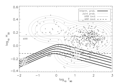
Figure 8.— Contour plot of the duration-hardness distribution based on the EEI model with three components in light-gray. Points show individual bursts. The broken lines in black show the probability contours of a given region belonging to the intermediate population. Also bursts classified as XRFs and XRR GRBs are marked on the plot with horizontal lines. One can observe a remarkable coincidence between the XRFs and the third group as shown by the indicator function.

Sakamoto et al. (2008a) define XRFs as events with fluence ratio $S_{23}>1.32$. This translates to a hardness ratio $H_{32}<0.76$. This definition aims to transform the limit of XRFs and X-ray rich GRBs found with BeppoSAX and HeteII. The limit is found using a pseudo-burst with spectral parameters: $\alpha=-1,\beta=-2.5$ and $E_{\mathrm{peak}}=100$ keV for a Band spectrum (Band et al., 1993). Based on this definition we identify $24$ bursts from our $408$ burst sample. Table 7. contains data of bursts along with the probabilities that they belong to the third population. The average of these probabilities (i.e. the XRF belongs to the intermediate group) is $95\%$. This high value allows us to conclude that all XRFs belong to the intermediate group defined by the EEI model with high probability.

Table 7X-ray flashes as defined by Sakamoto et al. (2008a) and the probability that they belong to the intermediate group.

Name	$T_{90}[s]$	$H_{32}$	3rd group prob.
050416A	$2.50$	$0.48$	$1.00$
050714B	$46.70$	$0.73$	$0.80$
050815	$2.90$	$0.72$	$0.98$
050819	$37.70$	$0.62$	$0.98$
050824	$22.60$	$0.59$	$0.99$
051016B	$4.00$	$0.75$	$0.97$
060219	$62.10$	$0.68$	$0.89$
060428B	$57.90$	$0.67$	$0.91$
060512	$8.50$	$0.71$	$0.96$
060923B	$8.60$	$0.70$	$0.97$
060926	$8.00$	$0.68$	$0.98$
061218	$6.50$	$0.57$	$1.00$
070224	$34.50$	$0.75$	$0.80$
070330	$9.00$	$0.55$	$1.00$
070714A	$3.00$	$0.66$	$0.99$
070721A	$3.78$	$0.53$	$1.00$
080218A	$23.00$	$0.76$	$0.84$
080218B	$6.40$	$0.60$	$1.00$
080315	$64.00$	$0.66$	$0.92$
080520	$2.84$	$0.46$	$1.00$
080822B	$64.00$	$0.63$	$0.95$
081007	$8.00$	$0.69$	$0.98$
081109B	$128.00$	$0.70$	$0.72$
081211A	$3.44$	$0.72$	$0.98$

Based on Fig. 8. we propose that the members of the third component are probably the X-ray flashes. Therefore, using the model based classification method we can give probabilistic definition for the X-ray flashes based on the duration-hardness distribution. This definition defines $22$ additional bursts that belong to the intermediate population and hence to the XRFs.

All the X-ray flashes are in the region where the third component has the highest probability, but not all third component bursts can be unambiguously classified as X-ray flashes according to the Sakamoto et al. (2008a) criterion. In other words the third component in the EEI model contains all the X-ray flashes and some additional, very soft bursts.

To give further support to our point, we make a histogram with the hardness ratios of the bursts (see Figure 9). The vertical line represents the working definition of XRFs and the filled part of the histogram represents putative X-ray flashes identified as the third, soft class in this study. The limiting contours are not horizontal, as the centers of the long and intermediate classes have different $T_{90}$ values. Furthermore, there are some short XRFs $T_{90}\approx 1$s which are harder than the working definition limit.

The mechanism behind the X-ray flashes is still not clear. There are various scenarios that could produce these phenomena (e.g. dirty fireballs, inefficient internal shocks, structured jets with off-axis viewing angle, etc., for a review of the models see (Zhang, 2007)). A more precise experimental definition of XRFs can result in more stringent constraints on the models.

Figure 9.— Hardness distribution of the bursts in the sample. The filled portion marks the intermediate population. The vertical line shows the limit defined to identify X-ray flashes by Sakamoto et al. (2008a), it identifies $24$ XRFs. An additional $22$ XRFs are proposed by the model fit probabilities.

6.3. Relation to a recent study on groups of GRBs using Swift data

A recent work by Horváth et al. (2010) also confirmed the existence of the third class in the Swift database. Horváth et al. (2010) used a maximum likelihood fit with EM algorithm. In their model they applied no restrictions for the parameters of the ellipses. This can be related to the VVV model in the MClust package with maximum number of degrees of freedom. In our case the VVV model is disfavored because of the lower BIC value caused by the higher number of free parameters. However, one model (VEI) with only marginally lower BIC value than the best model has a similar structure as the one found by Horváth et al. (2010). We have constructed contingency tables comparing the common bursts in the Horváth et al. (2010) with the model based results. (see Tables 8 and 9 for the comparison with the EEI and VEI models)

The common sample with the Horváth et al. (2010) study consists of $324$ GRBs. According to the contingency table (Table 8) there are $31$ bursts which are classified as intermediate in both studies. The main difference between the classifications can be seen in the the total number of intermediate bursts: Horváth et al. (2010) classify $86$ bursts as intermediates, and this study finds only $32$ (according to the EEI model).

The other important question is the number of X-ray flashes in the two kinds of classifications. Using the Sakamoto et al. (2008a) definition there are $19$ X-ray flashes in the common sample. These belong without exception in the intermediate class with the highest probability according to both Horváth et al. (2010) and this study. In other words the $31$ bursts classified as intermediate by both Horváth et al. (2010) and this study, contains all the X-ray flashes. Horváth et al. (2010) classifies $55$ bursts in the intermediate class, whereas here we classify them as long. Based on this we can state that the model presented here is more efficient to identify the X-ray flashes with high probability. The ratio of X-ray flashes in the intermediate class is $59\%$ in the EEI model and $22\%$ in the Horváth et al. (2010) study.

The VEI model with a marginally lower BIC value has only $32$ off-diagonal elements in the contingency table (see Table 9) when compared to the Horváth et al. (2010) study. The structure revealed by this model is more similar to the one in Horváth et al. (2010). In this model all the $19$ X-ray flashes are also classified as intermediate. In this case the the number of intermediate bursts is $118$ which means there are many bursts classified as intermediate which are not X-ray flashes. The ratio of XRFs to intermediate class members is $16\%$.

Table 8Contingency table comparing the $324$ common bursts from Horváth et al. (2010) and the EEI solution used in this study. There are $19$ X-ray flashes in this sample all of which are classified as intermediate by both methods, i.e. they are included in the intermediate-intermediate field with $31$ elements.

		Horváth et al. (2010)    classification
		Short	Intermediate	Long	Total
	Short	24	0	0	24
Model based	Interm.	0	31	1	32
(EEI)	Long	0	55	213	268
	Total	24	86	214	324

Table 9Contingency table comparing the $324$ common bursts from Horváth et al. (2010) and the VEI model.

		Horváth et al. (2010)    classification
		Short	Intermediate	Long	Total
	Short	22	0	0	22
Model based	Interm.	2	86	30	118
(VEI)	Long	0	0	184	184
	Total	24	86	214	324

The reason for finding different group structure for the intermediate population lies in the fact that this group is significantly overlaid with the long population and it is very much sensitive to the mathematical approach used.

7. Conclusion

The results of this paper can be summarized as follows:

• We have established with multiple methods - in concordance with previous studies - that Swift GRB data can be best modelled using three populations. Both the model independent and the model based methods showed three groups with high significance.

• We found that the third population of GRBs, intermediate in duration and with the softest spectrum, has a peak-flux distribution that significantly differs from the other two classes. This group has the lowest average peak-flux.

• Furthermore, the redshifts of the intermediate population do not differ significantly from that of the long class, although their average redshift is lower. Considering this and their lower average peak-flux it indicates that the intermediate GRBs are inherently dimmer than the longer ones.

• We have also found evidence that the intermediate population is closely related to X-ray flashes: all the previously identified Swift X-ray flashes belong to the third, soft population. Therefore, we relate the intermediate class to the X-ray flashes. Thus, we give a new, probabilistic definition for this phenomenon.

References

- Bagoly et al. (1998) Bagoly, Z., Mészáros, A., Horváth, I., Balázs, L. G., & Mészáros, P. 1998, ApJ, 498, 342
- Bagoly et al. (2006) Bagoly, Z., et al. 2006, A&A, 453, 797
- Band et al. (1993) Band, D., et al. 1993, ApJ, 413, 281
- Chattopadhyay et al. (2007) Chattopadhyay, T., Misra, R., Chattopadhyay, A. K., & Naskar, M. 2007, ApJ, 667, 1017
- Dempster et al. (1977) Dempster, A., Laird, N., & Rubin, D. 1977, Royal statistical Society B, 39, 1
- Dermer et al. (1999) Dermer, C. D., Chiang, J., & Böttcher, M. 1999, ApJ, 513, 656
- Dezalay et al. (1996) Dezalay, J. P., Lestrade, J. P., Barat, C., Talon, R., Sunyaev, R., Terekhov, O., & Kuznetsov, A. 1996, ApJ, 471, L27
- Fishman et al. (1994) Fishman, G. J., et al. 1994, ApJS, 92, 229
- Fraley & Raftery (2000) Fraley, C., & Raftery, A. E. 2000, Journal of the American Statistical Association, 97, 611
- Gehrels et al. (2004) Gehrels, N., et al. 2004, ApJ, 611, 1005
- Gehrels et al. (2006) —. 2006, Nature, 444, 1044
- Hakkila et al. (2003) Hakkila, J., Giblin, T. W., Roiger, R. J., Haglin, D. J., Paciesas, W. S., & Meegan, C. A. 2003, ApJ, 582, 320
- Hartigan (1975) Hartigan, J. A. 1975, Clustering algorithms, Vol. xiii (Wiley New York,), 351
- Heise et al. (2001) Heise, J., in’t Zand, J., Kippen, R. M., & Woods, P. M. 2001, in Gamma-ray Bursts in the Afterglow Era, ed. E. Costa, F. Frontera, & J. Hjorth, 16
- Horváth (1998) Horváth, I. 1998, ApJ, 508, 757
- Horváth (2002) —. 2002, A&A, 392, 791
- Horváth (2009) —. 2009, Ap&SS, 323, 83
- Horváth et al. (2010) Horváth, I., Bagoly, Z., Balázs, L. G., de Ugarte Postigo, A., Veres, P., & Mészáros, A. 2010, ApJ, 713, 552
- Horváth et al. (2006) Horváth, I., Balázs, L. G., Bagoly, Z., Ryde, F., & Mészáros, A. 2006, A&A, 447, 23
- Horváth et al. (2008) Horváth, I., Balázs, L. G., Bagoly, Z., & Veres, P. 2008, A&A, 489, L1
- Huja et al. (2009) Huja, D., Mészáros, A., & Řípa, J. 2009, A&A, 504, 67
- Hullinger (2006) Hullinger, D. 2006, PhD thesis, University of Maryland, College Park, United States – Maryland Advisor: Sullivan, Greg
- Jakobsson et al. (2006) Jakobsson, P., et al. 2006, A&A, 447, 897
- Kippen et al. (2003) Kippen, R. M., Woods, P. M., Heise, J., in’t Zand, J. J. M., Briggs, M. S., & Preece, R. D. 2003, in American Institute of Physics Conference Series, Vol. 662, Gamma-Ray Burst and Afterglow Astronomy 2001: A Workshop Celebrating the First Year of the HETE Mission, ed. G. R. Ricker & R. K. Vanderspek, 244–247
- Kouveliotou et al. (1993) Kouveliotou, C., Meegan, C. A., Fishman, G. J., Bhat, N. P., Briggs, M. S., Koshut, T. M., Paciesas, W. S., & Pendleton, G. N. 1993, ApJ, 413, L101
- Krolik & Hawley (2010) Krolik, J. H., & Hawley, J. F. 2010, in Lecture Notes in Physics, Berlin Springer Verlag, Vol. 794, Lecture Notes in Physics, Berlin Springer Verlag, ed. T. Belloni, 265
- Liddle (2007) Liddle, A. R. 2007, MNRAS, 377, L74
- Lü et al. (2010) Lü, H., Liang, E., Zhang, B., & Zhang, B. 2010, ApjL submitted
- Mahalanobis (1936) Mahalanobis, P. C. 1936, Proceedings National Institute of Science, India, 2, 49
- Mazets et al. (1981) Mazets, E. P., et al. 1981, Ap&SS, 80, 3
- Mészáros (2006) Mészáros, P. 2006, Reports on Progress in Physics, 69, 2259
- Mukherjee et al. (1998) Mukherjee, S., Feigelson, E. D., Babu, G. J., Murtagh, F., Fraley, C., & Raftery, A. 1998, ApJ, 508, 314
- Murtagh & Heck (1987) Murtagh, F., & Heck, A., eds. 1987, Astrophysics and Space Science Library, Vol. 131, Multivariate Data Analysis
- Norris et al. (1984) Norris, J. P., Cline, T. L., Desai, U. D., & Teegarden, B. J. 1984, Nature, 308, 434
- Pásztor et al. (1993) Pásztor, L., Tóth, L. V., & Balázs, L. G. 1993, A&A, 268, 108
- Qin et al. (2010) Qin, Y., Gupta, A. C., Fan, J., Su, C., & Lu, R. 2010, Science in China G: Physics and Astronomy, 34
- R Development Core Team (2008) R Development Core Team. 2008, R: A Language and Environment for Statistical Computing, R Foundation for Statistical Computing, Vienna, Austria, ISBN 3-900051-07-0
- Sakamoto et al. (2008a) Sakamoto, T., et al. 2008a, ApJ, 679, 570
- Sakamoto et al. (2008b) —. 2008b, ApJS, 175, 179
- Schwarz (1978) Schwarz, G. 1978, Annals of Statistics, 6, 461
- Řípa et al. (2009) Řípa, J., Mészáros, A., Wigger, C., Huja, D., Hudec, R., & Hajdas, W. 2009, A&A, 498, 399
- Yang (1993) Yang, M. S. 1993, Mathematical and Computer Modelling, 18, 1
- Zhang (2007) Zhang, B. 2007, Chinese Journal of Astronomy and Astrophysics, 7, 1
- Zhang et al. (2009) Zhang, B., et al. 2009, ApJ, 703, 1696