1 Introduction

Axions have been studied along the years both as a realistic attempt to solve the strong CP problem [1, 2],[3, 4, 5, 6, 7][8], to which they are closely related, but also as a possible candidate to answer more recent puzzles in cosmology, such as the origin of dark energy, whose presence has found confirmation in the study of Type I supernovae [9, 10]. In this second case it has been pointed out that they can contribute to the vacuum energy, a possibility that remains realistic if their mass $m_{a}$ - which in this case should be $\sim 10^{-33}$ eV and smaller - is of electroweak [11] and not of QCD origin. In this case they differ significantly from the standard (Peccei-Quinn, PQ) invisible axion.

According to this scenario, the vacuum misalignment (see [12, 13] for a discussion in the PQ case) induced at the electroweak scale would guarantee that the degree of freedom associated with the axion field remains frozen, rolling down very slowly towards the minimum of the non-perturbative instanton potential, with $m_{a}$ much smaller than the current Hubble rate. Given the rather tight experimental constraints which have significantly affected the parameter space (axion mass and gauge couplings) for PQ axions [14, 15, 16], the study of these types of fields has also taken into account the possibility to evade the current bounds [17, 18]. These are summarized both into an upper and a lower bound on the size of $f_{a}$, the axion decay constant, which sets the scale of the misalignment angle $\theta$, defined as the ratio of the axion field ($a$) over the PQ scale $v_{PQ}$ ($v_{PQ}\sim f_{a}$).

Axion-like particles can be reasonably described by pseudoscalar fields characterized by an enlarged parameter space for mass and couplings, with a direct coupling to the gauge fields (of the form $aF\tilde{F}$) whose strength remains unrelated to their mass. They have been at the center of several recent and less recent studies (see for instance [19, 20] [21, 22, 23, 18, 24, 25]). They are supposed to inherit most of the properties of a typical invisible axion - a PQ axion - while acquiring some others which are not allowed to it.

We recall that the axion mass (which in the PQ case is $O(\Lambda_{QCD}^{2}/f_{a})$ and the axion coupling to the gauge fields are indeed related by the same constant $f_{a}$. In the PQ case $f_{a}$ ($\sim 10^{10}-10^{12}$ GeV) makes the axion rather light ($\sim 10^{-3}-10^{-5}$ eV) and also very weakly coupled. The same (large) scale plays a significant role in establishing the axion as a possible dark matter candidate, contributing significantly to the relic densities of cold dark matter. A much smaller value of $f_{a}$, for instance, would diminish significantly the axion contribution to cold dark matter due to the suppression of its abundance ($Y_{\chi}$) which depends quadratically on $f_{a}$.

It is quite immediate to realize that the gauging of the axionic symmetries by introducing a local anomalous $U(1)$ - inherited from an underlying anomalous structure, i.e. a gauge anomaly - allows to leave the mass and the coupling of the axion to the gauge fields unrelated [26, 27], offering a natural theoretical justification for the origin of axion-like particles. We just recall that effective low energy models incorporating gauged PQ interactions emerge in several string and supergravity constructions, for instance in orientifold vacua of string theory and in gauged supergravities (see for instance [28, 29]).

The analysis that we perform in this work has the goal to capture the relevant phenomenological features of the axions present in this class of models, extending a previous study presented in a non-supersymmetric context [30]. We will be following, as in previous studies, a bottom-up approach. This allows to identify the low energy effective action on the basis of a rather simple operatorial structure typical of anomalous abelian models. The theory is then fixed by the condition of gauge invariance of the anomalous effective action, amended by operators of dimension-5 (Wess-Zumino or PQ-like terms) which appear in the action suppressed by a suitable scale, the Stückelberg mass ($M_{St}$).

The introduction of the Stückelberg multiplet (or axion multiplet), while necessary for the restoration of gauge invariance, is in general expected to raise some concerns at cosmological level because of the presence, among its components, of a scalar modulus, the saxion. In supersymmetric (ordinary) PQ formulations this has a mass of the order of the weak scale or smaller and poses severe problems to the standard cosmological scenario. A late time decay of this particle, for instance, could cause an entropy release with a low reheating temperature ($T_{RH}<5\,\textrm{MeV}$) which is unacceptable for nucleosynthesis. Just for comparison, we mention that in the case of string moduli, for instance, the interaction of these states with the rest of the fields of the low energy spectrum is suppressed by the Planck scale. In turn, this forces the mass of these states to be quite large (100 TeV or so) [31, 32] in order to enhance the phase space for their decay, for a similar reason.

In our construction the scalar modulus of the axion multiplet acquires a mass of the order of the Stückelberg scale and has sizeable interactions with the other fields of the model, thereby decaying pretty fast ($\sim 10^{-23}s$). Therefore, smaller values of its mass - in the TeV range - turn out to be compatible with the standard scenario for nucleosynthesis.

1.1 The USSM-A

Non-supersymmetric versions of the class of models that we are going to analyze have been discussed in details in [33, 26, 27]. Recently [34, 35], an extension of a specific supersymmetric model, the USSM (the $U(1)$-extended Next-to-Minimal Supersymmetric Standard Model of [36]) has been presented, in which the $U(1)$ symmetry is anomalous. This model supports an axion-like particle in its spectrum. It has been named the “USSM-A”, to recall both its supersymmetric origin and its anomalous abelian gauge structure. It is also close to a similar $U(1)^{\prime}$ extension of the MSSM (the $U(1)^{\prime}$ Minimal Supersymmetric Standard Model) [37], which supports an axino component among the interaction eigenstates of the neutralino sector, but not a gauged axion, due to the structure of the MSSM superpotential. The study of relic densities in this model have been performed in [38, 39]. In the non-supersymmetric case the identification of a physical axion in the spectra of these models has been discussed in detail in [33], a realization called “the Minimal Low Scale Orientifold Model” or MLSOM for short.

Both in the USSM-A and in the model of [37], the extra $U(1)$ symmetry takes an anomalous form and the violation of gauge invariance requires supersymmetric PQ interactions, with a Stückelberg supermultiplet for the restoration of the gauge symmetry. The extra gauge boson of the anomalous $U(1)$ symmetry is massive and in the Stückelberg phase, as in previous non-supersymmetric constructions [33, 26, 27]. As shown in the case of the MLSOM, axion-like particles appear in the CP-odd spectrum of these theories whenever Higgs-axion mixing [33] occurs. For this reason in this work we will be using the term “gauged supersymmetric axion” (or axi-Higgs, denoted equivalently as $\chi$ or $H_{0}^{5}$) to refer to this state.

As we have mentioned in the introduction, we will follow a minimal approach. This approach allows to define an effective theory on the basis of 1) an assigned gauge structure (the number of anomalous abelian interactions); 2) some conditions of anomaly cancellation and gauge invariance of the effective Lagrangian; 3) the choice of a suitable value of the Stückelberg mass scale characterizing the range in which the description of these effective models is compatible with unitarity [40]. As in a previous analysis for the LHC in the MLSOM [41], we will first stress on the general features of these models, deriving the defining conditions for the counterterms which appear in the structure of the effective action, before moving to a specific realization with a selected charge assignment. In our simulations we have found that the dependence of the results on the choices of the independent charges is, however, extremely mild. In this respect the properties that we are able to extrapolate from this class of models - even with a single charge assignment - are pretty general and depend quite sensitively only on the choice of the Stückelberg mass $M_{St}$ and the MSSM Higgs vev ratio $\tan\beta$.

In this section we will focus on the axion/saxion Lagrangian, leaving a general discussion of the various contributions to an appendix. It is given by

$${\cal L}_{axion/saxion}={\cal L}_{St}+{\cal L}_{WZ}$$ (1)

where ${\cal L}_{St}$ is the supersymmetric version of the Stückelberg mass term [42], while ${\cal L}_{WZ}$ denotes the WZ counterterms responsible for the axion-like nature of the pseudoscalar $b$. Specifically

$${\cal L}_{St} =\frac{1}{2}\int d^{4}\theta(\hat{{\bf b}}+\hat{{\bf b}}^{\dagger}+\sqrt{2}M_{St}\hat{B})^{2}$$

$${\cal L}_{WZ} =-\frac{1}{2}\int d^{4}\theta\left\{\left[\frac{c_{G}}{M_{St}}\,\textrm{Tr}({\cal G}{\cal G})\hat{{\bf b}}+\frac{c_{W}}{M_{St}}\,\textrm{Tr}(WW)\hat{{\bf b}}\right.\right.$$

$$\left.\left.+\frac{c_{Y}}{M_{St}}\hat{{\bf b}}W^{Y}_{\alpha}W^{Y,\alpha}+\frac{c_{B}}{M_{St}}\hat{{\bf b}}W^{B}_{\alpha}W^{B,\alpha}+\frac{c_{YB}}{M_{St}}\hat{{\bf b}}W^{Y}_{\alpha}W^{B,\alpha}\right]\delta(\bar{\theta}^{2})+h.c.\right\},$$ (2)

where we have denoted with $\cal{G}$ the supersymmetric field-strength of $SU(3)_{c}$, with $W$ the supersymmetric field-strength of $SU(2)$, with $W^{Y}$ and with $W^{B}$ the supersymmetric field-strength of $U(1)_{Y}$ and $U(1)_{B}$ respectively. The Lagrangian ${\mathcal{L}}_{St}$ is invariant under the $U(1)_{B}$ gauge transformations

$$\delta_{B}\hat{B}= \hat{\Lambda}+\hat{\Lambda}^{\dagger}$$

$$\delta_{B}\hat{\bf{b}}= -2M_{St}\hat{\Lambda}$$ (3)

where $\hat{\Lambda}$ is an arbitrary chiral superfield. So the scalar component of $\hat{\bf{b}}$, that consists of the saxion and the axion field, shifts under a $U(1)_{B}$ gauge transformation.
The coefficients $c_{I}\equiv(c_{G},c_{W},c_{Y},c_{B},c_{YB})$ are dimensionless, fixed by the conditions of gauge invariance, and are functions of the free charges $B_{i}$ of the model (as shown below in Eq. (5)). Extracting the group factors we have

$$c_{B}=-\frac{{\cal A}_{BBB}}{384\pi^{2}}\qquad\qquad c_{Y}=-\frac{{\cal A}_{BYY}}{128\pi^{2}}\qquad\qquad c_{YB}=-\frac{{\cal A}_{BBY}}{128\pi^{2}}$$

$$c_{W}=-\frac{{\cal A}_{BWW}}{64\pi^{2}}\qquad\qquad c_{G}=-\frac{{\cal A}_{BGG}}{64\pi^{2}}.$$ (4)

The coefficients ${\cal A}$ are defined by the conditions of gauge invariance of the effective action, related to the anomalies $\left\{U(1)_{B}^{3}\right\}$, $\left\{U(1)_{B},U(1)_{Y}^{2}\right\}$, $\left\{U(1)_{B}^{2},U(1)_{Y}\right\}$, $\left\{U(1)_{B},SU(2)^{2}\right\}$, $\left\{U(1)_{B},SU(3)^{2}\right\}$. Using the conditions of gauge invariance these coefficients assume the form

$${\cal A}_{BBB} =-3B_{H_{1}}^{3}-3B_{H_{1}}^{2}(3B_{L}+18B_{Q}-7B_{S})-3B_{H_{1}}(3B_{L}^{2}+(18B_{Q}-7B_{S})B_{S})$$

$$+3B_{L}^{3}+B_{S}(27B_{Q}^{2}-27B_{S}B_{Q}+8B_{S}^{2})$$

$${\cal A}_{BYY} =\frac{1}{2}(-3B_{L}-9B_{Q}+7B_{S})$$

$${\cal A}_{BBY} =2B_{H_{1}}(3B_{L}+9B_{Q}-5B_{S})+(12B_{Q}-5B_{S})B_{S}$$

$${\cal A}_{BWW} =\frac{1}{2}(3B_{L}+9B_{Q}-B_{S})$$

$${\cal A}_{BGG} =\frac{3}{2}B_{S}.$$ (5)

We have expressed all the anomaly equations in terms of 4 charges, $B_{i}\equiv(B_{H_{1}},B_{S},B_{Q},B_{L})$ ordered from 1 to 4 (left to right), which are defined in Tab. 2. Notice that these charges can be taken as fundamental parameters of the model. Their independent variation allows to scan the entire spectra of these models with no reference to any specific construction. These relations appear in the anomalous variation $(\delta_{B})$ of the supersymmetric 1-loop effective action of the model, which forces the introduction of supersymmetric PQ-like interactions (WZ terms) for its overall vanishing. Formally we have the relation

$$\delta_{B}(B_{i}){\mathcal{S}}_{\it 1loop}+\delta_{B}(c_{I}(B_{i})){\mathcal{S}}_{WZ}=0,$$ (6)

where the anomalous variation can be parameterized by the 4 charges $B_{i}$ together with the coefficients $c_{J}(B_{i})$ in front of the WZ counter-terms. In these notations, the uppercase index $J$ runs over all the 5 mixed-anomaly conditions $B^{3},BY^{2},B^{2}Y,BW^{2},BG^{2}$, ordered from 1 to 5 (left to right).
Before coming to the definition of the charge assignments we pause for a remark. As we are going to show in the next sections, the scalar potential takes a nonlocal form unless all the anomaly coefficients in Eq. 5 are zero. Such potential can however be expanded in powers of $\textrm{Re}b/M_{St}$, and as such these contributions turn out to be irrelevant if $M_{St}$ is a very large scale. The situation is rather different if $M_{St}$ is bound to lay around the 1 TeV region, where the potential could actually develope a singularity. In fact, in this case, it is in general expected that a singular potential will soon dominate the dynamics of the model.

We will give the explicit expression of the $D$-terms for a general choice of the counterterms. The function ($f$) which allows to identify all the charges in terms of the free ones is formally given by

$$f(B_{Q},B_{L},B_{H_{1}},B_{S})=(B_{Q},B_{U_{R}},B_{D_{R}},B_{L},B_{R},B_{H_{1}},B_{H_{2}},B_{S}).$$ (7)

These depend only upon the 4 free parameters $B_{Q},B_{L}$, $B_{H_{1}}$ and $B_{S}$. In our analysis, the charges of Eq. (7) have been assigned as

$$f(2,1,-1,3)=(2,0,-1,1,0,-1,-2,3).$$ (8)

As we have already mentioned, the dependence of our results on this choice of thi parametric charges is very small. Instead, as we will see, the relevant parameters of our analysis turn out to be: 1) the anomalous coupling of the gauge boson $g_{B}$, which controls the decay rate of the saxion and of the axion and 2) the Stückelberg mass.

2 Axions, saxions and all orders interactions

The contributions of the axion and saxion to the total Lagrangian are derived from the combination of the Stückelberg and Wess-Zumino terms. The complete axion/saxion Lagrangian expressed in terms of component fields is given by

$${\cal L}_{axion/saxion}\equiv{\cal L}_{St}+{\cal L}_{WZ}$$ (9)

and contains a mixing among the $D$-terms which is rather peculiar, as we are going to show. The off-shell expression of this Lagrangian is given by

$${\cal L}_{axion/saxion}=\frac{1}{2}\left(\partial_{\mu}\textrm{Im}\,b+M_{st}B_{\mu}\right)^{2}+\frac{1}{2}\partial_{\mu}\textrm{Re}b\,\partial^{\mu}\textrm{Re}b+\frac{i}{2}\psi_{\bf b}\sigma^{\mu}\partial_{\mu}\bar{\psi_{\bf b}}+\frac{i}{2}\bar{\psi_{\bf b}}\bar{\sigma}^{\mu}\partial_{\mu}\psi_{\bf b}+F_{\bf b}^{\dagger}F_{\bf b}+{\cal L}_{axion,i}$$ (10)

where the expression of ${\cal L}_{axion,i}$ is quite lengthy and can be found in the appendix (Eq. (86)).

The equation of motion for the auxiliary field $F_{\bf b}$ can be derived quite immediately and give for the $F-$term of the Stückelberg field the expression

$$F_{\bf b}=-\frac{1}{16}\frac{c_{G}}{M_{St}}\bar{\lambda}^{a}_{G}\bar{\lambda}^{a}_{G}-\frac{1}{16}\frac{c_{W}}{M_{St}}\bar{\lambda}^{i}_{W}\bar{\lambda}^{i}_{W}-\frac{1}{2}\frac{c_{Y}}{M_{St}}\bar{\lambda}_{Y}\bar{\lambda}_{Y}-\frac{1}{2}\frac{c_{B}}{M_{St}}\bar{\lambda}_{B}\bar{\lambda}_{B}+\frac{1}{2}\frac{c_{YB}}{M_{St}}\bar{\lambda}_{Y}\bar{\lambda}_{B}.$$ (11)

One important feature of the supersymmetric model is that $b$ is a complex field with its real and imaginary parts. While $\textrm{Im}\,b$ may appear in the CP-odd part of the scalar sector and undergoes mixing with the Higgs sector, its real part, $\textrm{Re}\,b$, the saxion (or scalar axion) before the EW symmetry breaking, has a mass exactly equal to the Stückelberg mass, as expected from supersymmetry. We just recall that in the absence of SUSY breaking parameters, the components of the Stückelberg multiplet form, together with the vector multiplet of the anomalous gauge boson, a massive vector multiplet of mass $M_{St}$. This is composed of the massive anomalous gauge boson, whose mass is given by the Stückelberg term, the massive saxion and a massive Dirac fermion of mass $M_{St}$. The fermion is obtained by diagonalizing the 2-dimensional mass matrix constructed in the basis of $\lambda_{B}$ - the gaugino from the vector multiplet $\hat{B}$ - and $\psi_{b}$, which is the axino of the Stückelberg multiplet. The diagonalization of this matrix trivially gives two Weyl eigenstates of the same mass $M_{St}$, which can be assembled into a single massive Dirac fermion of the same mass. Notice that in this re-identification of the degrees of freedom contained in $\hat{\bf b}$ and in the vector multiplet $\hat{B}$, $\textrm{Im}\,b$ takes the role of a Nambu-Goldstone mode and can be gauged away.

The saxion has typical interactions of the form $\textrm{Re}\,b\,F_{i}F_{j}$, with the gauge fields which have mixed-anomalies with $U(1)_{B}$, beside non-polynomial interactions with the remaining fields of the theory. As we are going to elaborate, this features shows up because of the presence of terms consisting of the product of two $D$ fields and the saxion. To clarify this point, we recall that the general Lagrangian contains a supersymmetric Wess-Zumino term of the form

$${\cal L}_{WZ,Y}=-\frac{1}{2}\int d^{4}\theta\;\frac{c_{Y}}{M_{St}}\hat{{\bf b}}W^{Y}_{\;\alpha}W^{Y\;\alpha}\;\delta(\bar{\theta}^{2})+h.c.$$ (12)

which gives, after the expansion in components, a term proportional to

$$\frac{c_{Y}}{M_{St}}\;\textrm{Re}b\;D_{Y}D_{Y}.$$ (13)

This kind of terms, once that the equations of motion (EOM) of the auxiliary fields D are calculated and substituted back into the lagrangian, give the non-polynomial form of the potential. Furthermore, from the WZ term corresponding to the anomaly $BBY$ (which is the term proportional to $c_{YB}$), we get a term proportional to $\textrm{Re}b\;D_{Y}D_{B}$ so that the EOM for the abelian D fields are coupled.
The derivation of such equations involves all the terms of the Lagrangian discussed in appendix A. We obtain

$$D_{B,OS}= \frac{1}{12+12\sqrt{2}\textrm{Re}b(c_{B}+c_{Y})/M_{St}-6\textrm{Re}b^{2}(c_{YB}^{2}-4c_{Y}c_{B})/M_{St}^{2}}$$

$$\bigg{\{}\left[2\frac{c_{B}}{M_{St}}\left(\sqrt{2}+2\frac{c_{Y}}{M_{St}}\textrm{Re}b\right)-\frac{c_{YB}^{2}}{M_{St}^{2}}\textrm{Re}b\right](-3i\lambda_{B}\psi_{\bf b}+h.c.)-12M_{St}\textrm{Re}b-12\sqrt{2}c_{Y}\textrm{Re}b^{2}+$$

$$12g_{B}\left(1+\sqrt{2}\frac{c_{Y}}{M_{St}}\textrm{Re}b\right)\big{(}B_{S}S^{\dagger}S+B_{H_{1}}H_{1}^{\dagger}H_{1}+B_{H_{2}}H_{2}^{\dagger}H_{2}+B_{D_{R}}\tilde{D}_{R}^{\dagger}\tilde{D}_{R}+B_{U_{R}}\tilde{U}_{R}^{\dagger}\tilde{U}_{R}+$$

$$B_{Q}\tilde{Q}^{\dagger}\tilde{Q}+B_{R}\tilde{R}^{\dagger}\tilde{R}+B_{L}\tilde{L}^{\dagger}\tilde{L}\big{)}+3\sqrt{2}\frac{c_{YB}}{M_{St}}(i\lambda_{Y}\psi_{\bf b}+h.c.)+$$

$$\sqrt{2}\frac{c_{YB}}{M_{St}}g_{Y}\textrm{Re}b\big{(}-3H_{1}^{\dagger}H_{1}+3B_{H_{2}}H_{2}^{\dagger}H_{2}+2\tilde{D}_{R}^{\dagger}\tilde{D}_{R}-4\tilde{U}_{R}^{\dagger}\tilde{U}_{R}+\tilde{Q}^{\dagger}\tilde{Q}+6\tilde{R}^{\dagger}\tilde{R}-3\tilde{L}^{\dagger}\tilde{L}\big{)}\Big{\}}$$

$$D_{Y,OS}= \frac{1}{12+12\sqrt{2}\textrm{Re}b(c_{B}+c_{Y})/M_{St}-6\textrm{Re}b^{2}(c_{YB}^{2}-4c_{Y}c_{B})/M_{St}^{2}}$$

$$\Big{\{}3\;\frac{c_{YB}^{2}}{M_{St}^{2}}\;\textrm{Re}b(i\lambda_{Y}\psi_{\bf b}+h.c.)+3\sqrt{2}\;\frac{c_{YB}}{M_{St}}(i\lambda_{Y}\psi_{\bf b}+h.c.)-6\sqrt{2}\;c_{YB}\textrm{Re}b^{2}+$$

$$6\sqrt{2}\;\frac{c_{YB}}{M_{St}}\;\textrm{Re}b\;g_{B}\big{(}B_{S}S^{\dagger}S+B_{H_{1}}H_{1}^{\dagger}H_{1}+B_{H_{2}}H_{2}^{\dagger}H_{2}+B_{D_{R}}\tilde{D}_{R}^{\dagger}\tilde{D}_{R}+B_{U_{R}}\tilde{U}_{R}^{\dagger}\tilde{U}_{R}+$$

$$B_{Q}\tilde{Q}^{\dagger}\tilde{Q}+B_{R}\tilde{R}^{\dagger}\tilde{R}+B_{L}\tilde{L}^{\dagger}\tilde{L}\big{)}-6\frac{c_{Y}}{M_{St}}\left(\sqrt{2}+2\frac{c_{B}}{M_{St}}\;\textrm{Re}b_{B}\right)(i\lambda_{Y}\psi_{\bf b}+h.c.)+$$

$$2g_{B}\left(1+\sqrt{2}\frac{c_{B}}{M_{St}}\textrm{Re}b\right)(-3H_{1}^{\dagger}H_{1}+3B_{H_{2}}H_{2}^{\dagger}H_{2}+2\tilde{D}_{R}^{\dagger}\tilde{D}_{R}-4\tilde{U}_{R}^{\dagger}\tilde{U}_{R}+\tilde{Q}^{\dagger}\tilde{Q}+6\tilde{R}^{\dagger}\tilde{R}-3\tilde{L}^{\dagger}\tilde{L})\Big{\}},$$ (14)

showing that their on-shell expressions are characterized by the appearance of the saxion field in a non-polynomial form.

Figure 1: Saxion interactions to lowest order in $1/M_{St}$. An infinite number of additional higher order interactions (in powers of $1/M_{St}$) are generated by the insertion on these vertices of $n$ powers of saxion lines. We use the double line notation for Majorana particles.

The presence of the Stückelberg mass allows to perform an expansion of these terms to all orders in $\textrm{Re}\,b/M_{St}$. The first terms of the series expansion are given by

$$\frac{1}{12+12\sqrt{2}\textrm{Re}b(c_{B}+c_{Y})/M_{St}-6\textrm{Re}b^{2}(c_{YB}^{2}-4c_{Y}c_{B})/M_{St}^{2}}=$$

$$\frac{1}{12}-c_{Y}\frac{\textrm{Re}b}{6\sqrt{2}M_{St}}-c_{B}\frac{\textrm{Re}b}{6\sqrt{2}M_{St}}+\frac{1}{6}c_{Y}^{2}\frac{\textrm{Re}b^{2}}{M_{St}^{2}}+\frac{1}{24}c_{YB}^{2}\frac{\textrm{Re}b^{2}}{M_{St}^{2}}+\frac{1}{6}c_{B}^{2}\frac{\textrm{Re}b^{2}}{M_{St}^{2}}+\frac{1}{6}c_{B}c_{Y}\frac{\textrm{Re}b^{2}}{M_{St}^{2}}+O(\textrm{Re}b^{2}/M_{St}^{2})$$ (15)

We present a list of the vertices to leading order in $1/M_{St}$ in Fig. 1. Additional vertices (not shown) come with $n$ insertions of $\textrm{Re}\,b$ and a suppression by higher powers $(2\,n)$ of $M_{St}$. Some considerations are in order concerning the allowed values of $M_{St}$. A very large Stückelberg mass, in principle, would be sufficient to guarantee that the effect of reheating - caused by the decay of the saxion - takes place well above the temperature of nucleosynthesis (see for instance the discussion in [32]) thereby avoiding the problem of a possible late entropy release at that time. In this case one can essentially neglect the saxion from the low energy spectrum. For moduli of string origin the required mass value ($\sim 100$ TeV), much larger than in our case, is justified by the suppressed gravitational interaction of the modulus with the rest of the matter fields and works as an enhancing factor for its decay. In our case, instead, such a suppression is absent and a fast decay of the saxion is guaranteed already by a Stückelberg mass around the TeV scale.

3 The scalar potential and the saxion

As we have mentioned, in this model there are three scalar fields which take a vev, $H_{1},H_{2}$ and $S$, the scalar components of the scalar superfield $\hat{S}$. We assume that also the saxion field gets a vev, $v_{b}$. The scalar potential is composed by contributions coming from the $D$-terms, $F$-terms and scalar mass terms. Expanding up to $O(\textrm{Re}b/M_{St})$ we find

$$V=|\lambda H_{1}\cdot H_{2}|^{2}+|\lambda S|^{2}(|H_{1}|^{2}+|H_{2}|^{2})+m_{1}^{2}|H_{1}|^{2}+m_{2}^{2}|H_{2}|^{2}+m_{S}^{2}|S|^{2}+(a_{\lambda}SH_{1}\cdot H_{2}+h.c.)-$$

$$\frac{1}{8}g_{Y}^{2}\left(H_{1}^{\dagger}H_{1}-H_{2}^{\dagger}H_{2}\right)^{2}-\frac{1}{2}g_{B}^{2}\left(B_{H_{1}}H_{1}^{\dagger}H_{1}+B_{H_{2}}H_{2}^{\dagger}H_{2}+B_{S}S^{\dagger}S\right)^{2}-$$

$$\frac{1}{8}g_{2}^{2}\left[\left(H_{1}^{\dagger}H_{1}-H_{2}^{\dagger}H_{2}\right)^{2}+4|H_{1}^{\dagger}H_{2}|^{2}\right]+$$

$$\textrm{Re}b^{3}\left[\frac{c_{B}M_{St}}{\sqrt{2}}+g_{Y}\frac{\left(c_{Y}+c_{B}\right)c_{YB}}{2M_{St}}\left(H_{1}^{\dagger}H_{1}-H_{2}^{\dagger}H_{2}\right)\right]-$$

$$\textrm{Re}b^{2}\bigg{[}\frac{m_{\textrm{Re}b}^{2}}{2}+\frac{M_{St}^{2}}{2}+\sqrt{2}\;c_{B}\;g_{B}\left(B_{H_{1}}H_{1}^{\dagger}H_{1}+B_{H_{2}}H_{2}^{\dagger}H_{2}+B_{S}S^{\dagger}S\right)+\frac{c_{YB}\;g_{B}}{2\sqrt{2}}\left(H_{1}^{\dagger}H_{1}-H_{2}^{\dagger}H_{2}\right)\bigg{]}+$$

$$\textrm{Re}b\bigg{\{}g_{B}M_{St}\left(B_{H_{1}}H_{1}^{\dagger}H_{1}+B_{H_{2}}H_{2}^{\dagger}H_{2}+B_{S}S^{\dagger}S\right)+\frac{c_{W}g_{2}}{32\sqrt{2}M_{St}}\left[\left(H_{1}^{\dagger}H_{1}-H_{2}^{\dagger}H_{2}\right)^{2}+4|H_{1}^{\dagger}H_{2}|^{2}\right]+$$

$$\frac{c_{Y}g_{Y}^{2}}{4\sqrt{2}M_{St}}\left(H_{1}^{\dagger}H_{1}-H_{2}^{\dagger}H_{2}\right)^{2}+\frac{c_{B}g_{B}^{2}}{\sqrt{2}M_{St}}\left(B_{H_{1}}H_{1}^{\dagger}H_{1}+B_{H_{2}}H_{2}^{\dagger}H_{2}+B_{S}S^{\dagger}S\right)^{2}+$$

$$\frac{c_{YB}\,g_{Y}g_{B}}{2\sqrt{2}M_{St}}\left(B_{H_{1}}H_{1}^{\dagger}H_{1}+B_{H_{2}}H_{2}^{\dagger}H_{2}+B_{S}S^{\dagger}S\right)\left(H_{1}^{\dagger}H_{1}-H_{2}^{\dagger}H_{2}\right)\bigg{\}}.$$ (16)

To proceed with the analysis of this potential we introduce the following parameterizations

$$H_{1}=\frac{1}{\sqrt{2}}\begin{pmatrix}\textrm{Re}H_{1}^{0}+i\leavevmode\nobreak\ \textrm{Im}H_{1}^{0}\\ \textrm{Re}H_{1}^{-}+i\leavevmode\nobreak\ \textrm{Im}H_{1}^{-}\end{pmatrix}\hskip 14.22636ptH_{2}=\frac{1}{\sqrt{2}}\begin{pmatrix}\textrm{Re}H_{2}^{+}+i\leavevmode\nobreak\ \textrm{Im}H_{2}^{+}\\ \textrm{Re}H_{2}^{0}+i\leavevmode\nobreak\ \textrm{Im}H_{2}^{0}\end{pmatrix}\hskip 14.22636ptS=\frac{1}{\sqrt{2}}(\textrm{Re}S+i\leavevmode\nobreak\ \textrm{Im}S).\\$$

expanded around the vevs of the Higgs fields and of the saxion as

$$\left\langle H_{1}\right\rangle=\frac{1}{\sqrt{2}}\left(\begin{array}[]{c}v_{1}\\ 0\end{array}\right)\hskip 28.45274pt\left\langle H_{2}\right\rangle=\frac{1}{\sqrt{2}}\left(\begin{array}[]{c}0\\ v_{2}\end{array}\right)\hskip 28.45274pt\tan\beta=\frac{v_{2}}{v_{1}}\hskip 28.45274pt\left\langle S\right\rangle=\frac{v_{S}}{\sqrt{2}}\hskip 28.45274pt\left\langle\textrm{Re}b\right\rangle=\frac{v_{b}}{\sqrt{2}}.$$ (21)

The scalar mass parameters can be expressed in terms of the remaining parameters of the theory using the minimization conditions for the scalar potential. In particular, taking a derivative of the potential with respect to the saxion field we get the relation

$$\frac{\partial V}{\partial\textrm{Re}b}=-v_{b}m_{\textrm{Re}b}^{2}-v_{b}M_{St}^{2}+\frac{1}{2}g_{B}M_{St}B_{H_{1}}v_{1}^{2}+\frac{1}{2}g_{B}M_{St}B_{H_{2}}v_{2}^{2}+\frac{1}{2}g_{B}M_{St}B_{S}v_{S}^{2}$$ (22)

where we have neglected all the contributions suppressed by the Stückelberg mass. We can use this relation as a necessary condition in order to express $m_{\textrm{Re}b}^{2}$ in terms of the vevs and of the other parameters of the scalar potential. A numerical analysis of the Hessian at this point, for the selected parameters of the model used in our simulations, shows that indeed this extremal point indeed corresponds to a minimum.

We will try to highlight the most interesting features of these types of models and the implications for the axion, which are all connected to the properties of the vacuum of these theories below the scale of SUSY breaking and at the scales of the electroweak and QCD phase transitions.

4 Saxion decay modes

Having summarized the basic structure of the model, we now turn to describe the leading contributions to the 2-body decays of the saxion . The goal of this analysis is to ensure that the decay rate of the saxion is such that it occurs fast enough in order not to interfere with the nucleosynthesys.

We will compute its decay rate by considering the worst possible scenario, i.e. by assuming that this decay occurs around the SUSY breaking scale, or temperature T around 1 TeV. At this temperature, the decays of the saxion are parameterized by the typical SUSY breaking scales such as $M_{b}$ and $M_{Y}$, both of O($M_{susy}$). The model is in a symmetric electroweak phase ($M_{susy}>v$), which justifies the use of the interaction eigenstates (rather than the mass eigenstates) for the description of the final decay products.

The relevant interactions for the saxion decay are described by the general Lagrangian

$${\mathcal{L}}_{saxiondec.}= \textrm{Re}\,b\left[g_{B}M_{St}\leavevmode\nobreak\ B_{H_{1}}H_{1}^{\dagger}H_{1}+g_{B}M_{St}\leavevmode\nobreak\ B_{H_{2}}H_{2}^{\dagger}H_{2}+g_{B}M_{St}\leavevmode\nobreak\ B_{S}S^{\dagger}S+\right.$$

$$\left.g_{B}M_{St}\leavevmode\nobreak\ B_{Q}\sum_{j=1}^{3}\tilde{Q}_{j}^{\dagger}\tilde{Q}_{j}+g_{B}M_{St}\leavevmode\nobreak\ B_{D_{R}}\sum_{j=1}^{3}\tilde{D}_{R,j}^{\dagger}\tilde{D}_{R,j}+g_{B}M_{St}\leavevmode\nobreak\ B_{U_{R}}\sum_{j=1}^{3}\tilde{U}_{R,j}^{\dagger}\tilde{U}_{R,j}+\right.$$

$$\left.g_{B}M_{St}\leavevmode\nobreak\ B_{L}\sum_{l=e,\mu,\tau}\tilde{L}_{l}^{\dagger}\tilde{L}_{l}+g_{B}M_{St}\leavevmode\nobreak\ B_{R}\sum_{l=e,\mu,\tau}\tilde{R}_{l}^{\dagger}\tilde{R}_{l}\right.$$

$$\left.-i\frac{c_{B}}{2\sqrt{2}}\left(\lambda_{B}\leavevmode\nobreak\ \psi_{\bf b}+\bar{\lambda}_{B}\leavevmode\nobreak\ \bar{\psi}_{\bf b}\right)-i\frac{c_{YB}}{2\sqrt{2}}\left(\psi_{\bf b}\leavevmode\nobreak\ \lambda_{Y}+\bar{\psi}_{\bf b}\leavevmode\nobreak\ \bar{\lambda}_{Y}\right)\right].$$ (23)

They involve CP-even and CP-odd massless scalars, the extra singlet scalar $S$, the squarks, the sleptons and the gauginos $\psi_{\bf b},\leavevmode\nobreak\ \lambda_{Y}$. We compute the total decay rate into fermions, squarks and sleptons, and Higgs scalars. The left-handed doublets of the squarks and the sleptons are defined as $\tilde{Q}_{j}$ and $\tilde{L}_{l}$ respectively, while the right-handed singlets are $\tilde{U}_{R,j}$, $\tilde{D}_{R,j}$ and $\tilde{R}_{l}$, with $j,l$ labeling the fermion families.

• Decays into fermions

Assuming that $M_{\bf b}\approx M_{Y}$ are slightly less than 1 TeV, the decay rates of the saxion into one gaugino and one axino are

$$\Gamma\left(\textrm{Re}\,b\rightarrow\bar{\lambda}_{B}\psi_{\bf b}\right)=c_{B}^{2}\frac{M_{\textrm{Re}\,b}}{32\pi}\left(1-4\frac{M_{\bf b}^{2}}{M_{\textrm{Re}b}^{2}}\right)^{3/2}\,,$$

$$\Gamma\left(\textrm{Re}\,b\rightarrow\bar{\lambda}_{Y}\psi_{\bf b}\right)=c_{YB}^{2}\frac{M_{\textrm{Re}\,b}}{32\pi}\left(1-4\frac{M_{Y}^{2}}{M_{\textrm{Re}b}^{2}}\right)^{3/2}$$ (24)

with the expressions of the coefficients $c_{B}$ and $c_{YB}$ determining the couplings given explicitly in Eq. (4). Notice that these rates are large due to the linear dependence on $M_{\textrm{Re}b}(=M_{St})$.

• Decays into Squarks and Sleptons

In this channel we consider, for simplicity, the decay only into squarks and sleptons of the same type. Even in this case we are assuming that the masses of the squarks and of the sleptons are all equal and slightly below 1 TeV. The decay rate into the $i$-type sfermion is given by

$$\Gamma\left(\textrm{Re}b\rightarrow\tilde{f}_{i}^{\dagger}\tilde{f}_{i}\right)=\frac{g_{i}^{2}\lambda^{1/2}}{16\pi M_{\textrm{Re}_{b}}^{3}}$$ (25)

where the kinematic function $\lambda$ is, in general, defined as $\lambda=\left(M_{i}^{2}+M_{j}^{2}-M_{\textrm{Re}_{b}}^{2}\right)^{2}-4M_{i}^{2}M_{j}^{2}$ (here with $M_{i}=M_{j}$), and the couplings $g_{i}$, in the various cases, are defined as

$$g_{i}=\left\{\begin{array}[]{rl}N_{c}\leavevmode\nobreak\ c_{U_{R}}&\textrm{R-handed singlet u-type squark},\\ N_{c}\leavevmode\nobreak\ c_{D_{R}}&\textrm{R-handed singlet quark d-type squark},\\ N_{c}\leavevmode\nobreak\ c_{Q_{L}}&\textrm{L-handed doublet squark},\\ c_{R}&\textrm{R-handed singlet slepton $\tilde{e},\tilde{\mu},\tilde{\tau}$},\\ c_{L}&\textrm{L-handed doublet slepton}.\end{array}\right.$$ (26)

Here $N_{c}=3$ is the color factor and the various couplings are given as

$$c_{D_{R}}=\frac{1}{2}g_{B}\leavevmode\nobreak\ M_{St}\leavevmode\nobreak\ B_{D_{R}},\hskip 14.22636ptc_{U_{R}}=\frac{1}{2}g_{B}\leavevmode\nobreak\ M_{St}\leavevmode\nobreak\ B_{U_{R}},\hskip 14.22636ptc_{Q_{L}}=-\frac{1}{2}g_{B}M_{St}\leavevmode\nobreak\ B_{Q},$$

$$c_{L}=-\frac{1}{2}g_{B}\leavevmode\nobreak\ M_{St}\leavevmode\nobreak\ B_{L},\hskip 14.22636ptc_{R}=\frac{1}{2}g_{B}\leavevmode\nobreak\ M_{St}\leavevmode\nobreak\ B_{R}.$$ (27)

• Decays into massless scalars

The decay rate into particles of the Higgs sector that we denote generically with $h_{i}=\textrm{Re}H_{1},\textrm{Im}H_{1},\dots$ is given by

$$\Gamma\left(\textrm{Re}\,b\rightarrow h_{i}h_{i}\right)=\frac{s_{i}^{2}}{32\pi M_{\textrm{Re}\,b}}\left(1-4\frac{M_{s_{i}}^{2}}{M_{\textrm{Re}\,b}^{2}}\right)^{1/2}\,,$$ (28)

where the couplings $s_{i}$ are defined as

$$s_{i}=\left\{\begin{array}[]{rl}c_{H_{1}}&\textrm{$H_{1}$ Higgs doublet}\\ c_{H_{2}}&\textrm{$H_{2}$ Higgs doublet}\\ c_{S}&\textrm{$S$ Higgs singlet}\end{array}\right.$$ (29)

and the coefficients $c_{H_{1}},c_{H_{2}},c_{S}$ are

$$c_{H_{1}}=-\frac{1}{4}g_{B}\leavevmode\nobreak\ M_{St}\leavevmode\nobreak\ B_{H_{1}},\hskip 28.45274ptc_{H_{2}}=-\frac{1}{4}g_{B}\leavevmode\nobreak\ M_{St}\leavevmode\nobreak\ B_{H_{2}},\hskip 28.45274ptc_{S}=-\frac{1}{4}g_{B}\leavevmode\nobreak\ M_{St}\leavevmode\nobreak\ B_{S}.$$ (30)

The total decay rate is obtained by summing over all the decay modes

$$\Gamma_{\textrm{tot}}=\Gamma\left(\textrm{Re}\,b\rightarrow\bar{\lambda}_{b}^{\prime}\psi_{\bf b}\right)+\Gamma\left(\textrm{Re}\,b\rightarrow\bar{\lambda}_{Y}\psi_{\bf b}\right)+\sum_{i}\Gamma\left(\textrm{Re}\,b\rightarrow\tilde{\bar{f}}_{i}\tilde{f}_{i}\right)+\sum_{i}\Gamma\left(\textrm{Re}\,b\rightarrow h_{i}h_{i}\right).$$ (31)

All the decay rates depend upon the value of the extra $U_{B}(1)$ coupling $g_{B}$, the Stückelberg mass $M_{St}$ and the SUSY breaking scale $M_{susy}$.

The total decay rate and the lifetime of the saxion are shown in Fig. (2), with the saxion mass $M_{\textrm{Re}b}$ given by the Stückelberg scale ($M_{\textrm{Re}b}=M_{St}$) around 1.4 TeV, and with all the squarks and the sleptons in the final state taken of a mass of 700 GeV. All the particles of the Higgs sector are considered to be massless. For $g_{B}=0.01$ we obtain a saxion whose decay rate is around 60 MeV if its mass is 1.7 TeV, and which decays rather quickly, since its lifetime is about $10^{-23}$ seconds. The lifetime decreases quite significantly as we increase the gauge coupling of the anomalous gauge symmetry. For instance, for $g_{B}=0.1$ it decreases to $\sim 10^{-24}$ sec, since the phase space for the decay is considerably enhanced.

We conclude that the saxion decays sufficiently fast and does not generate any late entropy release at the time of nucleosynthesis. Obviously, this scenario remains valid for all values of the Stückelberg mass above the 1 TeV value. Therefore, in the analysis of the evolution of the contributions to the total energy density ($\rho$) of the universe, either due to matter ($\rho_{m}$) or to radiation ($\rho_{R}$), at temperatures $T\leq 2$ TeV, the contribution coming from the saxion is entirely accounted for by $\rho_{R}$.

At this point, having cleared the way of any possible obstruction due to the presence of moduli at the low energy stage ($T\leq 2$ TeV) of the evolution of our model, we are ready to discuss the relevant features of the Stückelberg field. In particular, we will discuss the appearance of a physical axion, the physical component of the Stückelberg, at the electroweak scale. This is extracted from the CP-odd sector and generated by the mechanism of vacuum misalignment taking place at the same scale. In particular, the discussion serves to illustrate how a flat - but physical - direction might be singled out from the vacuum manifold, acquiring a small curvature at the electroweak phase transition.

Figure 2: Total decay rate and lifetime of the saxion for different values of $g_{B}$ as a function of the Stückelberg mass.

5 The flat direction of the physical axion from Higgs-axion mixing

In [34],[35] we have presented in some detail an approximate procedure in order to identify in the CP-odd sector one state that inherits axion-like interactions. The approach did not require the explicit expressions of the curvature terms in the CP-odd part of the supersymmetric potential, which are instead needed in the discussion of the angle of misalignment. Here we are going to extend this analysis by giving the explicit parameterization of these additional terms. The determination of the angle of misalignment and its parameterization in terms of the physical axion is based on an extension of the method presented in [30]. We are going to illustrate this point starting, for simplicity, from the non-supersymmetric case and then moving to the supersymmetric one.

5.1 The non-supersymmetric case

In the non-supersymmetric case the scalar sector contains two Higgs doublets $V_{PQ}(H_{u},H_{d})$ plus one extra contribution (a PQ breaking potential), denoted as $V_{P\kern-3.01389pt\hbox{/}Q\kern-3.01389pt\hbox{/}}(H_{u},H_{d},b)$, which mixes the Higgs sector with the Stückelberg axion $b$,

$$V=V_{PQ}(H_{u},H_{d})+V_{P\kern-3.01389pt\hbox{/}Q\kern-3.01389pt\hbox{/}}(H_{u},H_{d},b).$$ (32)

The mixing induced in the CP-odd sector determines the presence of a linear combination of the Stückelberg field $b$ and of the Goldstones of the CP-odd sector, called $\chi$, which is characterized by an almost flat direction, whose curvature is controlled by the strength of the extra potential $V_{P\kern-3.01389pt\hbox{/}Q\kern-3.01389pt\hbox{/}}$. $V_{PQ}(H_{u},H_{d})$ is the ordinary potential of 2 Higgs doublets,

$$V_{PQ}=\mu_{u}^{2}H_{u}^{\dagger}H_{u}+\mu_{d}^{2}H_{d}^{\dagger}H_{d}+\lambda_{uu}(H_{u}^{\dagger}H_{u})^{2}+\lambda_{dd}(H_{d}^{\dagger}H_{d})^{2}-2\lambda_{ud}(H_{u}^{\dagger}H_{u})(H_{d}^{\dagger}H_{d})+2\lambda^{\prime}_{ud}|H_{u}^{T}\tau_{2}H_{d}|^{2}$$

Concerning the $V_{P\kern-3.01389pt\hbox{/}Q\kern-3.01389pt\hbox{/}}$ contribution to the total potential, its structure is inferred just on the basis of gauge invariance and given by

$$V_{P\kern-3.01389pt\hbox{/}Q\kern-3.01389pt\hbox{/}}= \lambda_{0}(H_{2}^{\dagger}H_{1}e^{-ig_{B}(B_{H_{2}}-B_{H_{1}})\frac{b}{2M_{St}}})+\lambda_{1}(H_{2}^{\dagger}H_{1}e^{-ig_{B}(B_{H_{2}}-B_{H_{1}})\frac{b}{2M_{St}}})^{2}+$$

$$\lambda_{2}(H_{2}^{\dagger}H_{2})(H_{2}^{\dagger}H_{1}e^{-ig_{B}(B_{H_{2}}-B_{H_{1}})\frac{b}{2M_{St}}})+\lambda_{3}(H_{1}^{\dagger}H_{1})(H_{2}^{\dagger}H_{1}e^{-ig_{B}(B_{H_{2}}-B_{H_{1}})\frac{b}{2M_{St}}})+\textrm{h.c.}$$ (34)

These terms are the only ones allowed by the symmetry of the model and are parameterized by one dimensionful ($\lambda_{0}\equiv\bar{\lambda}_{0}v$) and three dimensionless constants $(\lambda_{1},\lambda_{2},\lambda_{3})$.

The CP-odd sector is then spanned by the three fields $(\textrm{Im}H_{1},\textrm{Im}H_{2},b)$, with the potential $V_{PQ}$ a function only of $H_{1}$ and $H_{2}$. After electroweak symmetry breaking, due to Higgs-axion mixing, $b$ can be written as a linear combination of a physical axion and of an extra component. The latter is a linear combination of the two Goldstone modes of the total potential $(V_{PQ}+V_{P\kern-3.01389pt\hbox{/}Q\kern-3.01389pt\hbox{/}})$, denoted as $G_{0}^{1},G_{0}^{2}$. The physical axion, $\chi$, i.e.  the component of $b$ which is not proportional to the two Goldstones, can be identified using the rotation matrix $O^{\chi}$ which relates interaction and mass eigenstates in the CP-odd sector

$$\begin{pmatrix}G_{0}^{1}\\ G_{0}^{2}\\ \chi\end{pmatrix}=O^{\chi}\begin{pmatrix}\textrm{Im}H^{0}_{1}\\ \textrm{Im}H^{0}_{2}\\ b\end{pmatrix}.$$ (35)

which takes the form

$$b=O_{13}^{\chi}G_{0}^{1}+O_{23}^{\chi}G_{0}^{2}+O_{33}^{\chi}\chi.$$ (36)

$\chi$ inherits WZ interactions from $b$ via Eq. (36), once this is introduced into the WZ counterterms.

From an explicit computation one finds that $O_{13}^{\chi}=0$, $O_{23}^{\chi}\sim O(1)$ and $O_{33}^{\chi}\sim v/M_{St}$. The Goldstones of the two neutral gauge bosons, $G_{Z},G_{Z^{\prime}}$ are linear combinations of $G_{0}^{1}$ and $G_{0}^{2}$ and can be extracted from the bilinear mixings after an expansion around the broken electroweak vacuum. Then, the entire CP-odd sector can be spanned by the basis $(G_{Z},G_{Z^{\prime}},\chi)$. The presence of an extra degree of freedom in this sector has been established in [33] using a simple counting of the degrees of freedom. We review this point for clarity.

There are 9 degrees of freedom in the set $(A_{Y},W_{3},B,\textrm{Im}H_{1},\textrm{Im}H_{2})$, where $B$ is the massive Stückelberg gauge vector field, before electroweak symmetry breaking, as well as 9 in the set $(A_{\gamma},Z,Z^{\prime},\chi)$, which is generated after the breaking. The direction determining the gauged axion $\chi$ is then physical but flat, in the absence of an extra potential which may depend explicitly on $b$. The potential $V^{\prime}$ is responsible for giving a small mass for $\chi$ and can be used to parameterize the mechanism of vacuum misalignment originated at the electroweak scale.

One can explore the structure of this potential and, in particular, investigate its periodicity. The phase of the potential is indeed parameterized by the ratio $\chi/\sigma_{\chi}$ [30]

$$V_{P\kern-3.01389pt\hbox{/}Q\kern-3.01389pt\hbox{/}}= 4v_{1}v_{2}\left(\lambda_{2}v_{1}^{2}+\lambda_{3}v_{2}^{2}+\lambda_{0}\right)\cos\left(\frac{\chi}{\sigma_{\chi}}\right)+2\lambda_{1}v_{1}^{2}v_{2}^{2}\cos\left(2\frac{\chi}{\sigma_{\chi}}\right)$$ (37)

with a mass for the physical axion $\chi$ given by

$$m_{\chi}^{2}=\frac{2v_{1}v_{2}}{\sigma^{2}_{\chi}}\left(\bar{\lambda}_{0}v^{2}+\lambda_{2}v_{1}^{2}+\lambda_{3}v_{2}^{2}+4\lambda_{1}v_{1}v_{2}\right)\approx\lambda_{eff}v^{2},$$ (38)

with $\sigma_{\chi}\sim O(v)$. The size of this expression is the result of two factors which appear in Eq. (38): the size of the potential, parameterized by $(\bar{\lambda}_{0},\lambda_{1},\lambda_{2},\lambda_{3})$, and the electroweak vevs of the two Higgses. The appearance of $\chi$ in Eq. (37) - in the phase of the extra potential - shows explicitly that the angle of misalignment is entirely described by this field. The angle is defined as

$$\theta(x)\equiv\frac{\chi(x)}{\sigma_{\chi}},$$ (39)

where

$$\sigma_{\chi}\equiv\frac{2v_{1}v_{2}M_{St}}{\sqrt{g_{B}^{2}(B_{H_{2}}-B_{H_{1}})^{2}v_{1}^{2}v_{2}^{2}+2M_{St}^{2}(v_{1}^{2}+v_{2}^{2})}}$$ (40)

is the new dimensionful constant which takes the same role of the scale $f_{a}$ of the PQ case $(\theta(x)=a/f_{a})$. The potential is characterized by a small strength $\sim\lambda_{eff}v^{4}$, and for this reason one can think of $\chi$ as a pseudo Nambu-Goldstone mode of the theory.

At this stage, it is important to realize that the size of the extra potential is significant in order to establish whether the degree of freedom associated to the axion field remains frozen or not at the electroweak scale. For instance, if $\lambda_{eff}$ is associated to electroweak instantons ($\lambda_{eff}\sim\lambda_{inst}$), then $m_{\chi}$ is very suppressed (see the discussion in Sec. 5.3) and far smaller than the corresponding Hubble rate at the electroweak scale

$$H(T)=\frac{1}{3}\sqrt{\frac{4}{5}\pi^{3}g_{*,T}}\frac{T^{2}}{M_{P}}$$ (41)

which is about $10^{-5}$ eV. In the expression above $g_{*,T_{i}}$ is the number of effective massless degrees of freedom of the model at a given temperature ($T$), while $M_{P}$ denotes the Planck mass. We recall that the condition

$$m_{\chi}(T)\sim 3H(T)$$ (42)

which ensures the presence of oscillations and determines implicitly the oscillation temperature $T_{i}$, is indeed impossible to satisfy if the misalignment that generates the value of $m_{\chi}$ at the electroweak scale is assumed of being of instanton origin (see the discussion in Appendix C). This implies that the degree of freedom associated to this physical axion would be essentially frozen at the electroweak scale, and the oscillations could take place at a later stage in the early universe, only around the QCD hadron transition. Instead, a more sizeable potential, providing an axion mass larger than $10^{-5}$ eV, would allow such oscillations. For an axion mass around 1 MeV oscillations indeed occur, but are damped by the particle decay, given that its lifetime ($\tau_{l}\sim 10^{-4}$ sec) is much larger than period of their oscillation ( $\tau_{osc}\sim 10^{-13}$ sec). This discussion is going to be expanded to the supersymmetric case.

5.2 Supersymmetry and the angle of misalignment

In the supersymmetric case the situation is analogous, in the sense that the physical direction $\chi$ can be identified by the same criteria. The superpotential that we are considering allows the presence of one extra degree of freedom, given by $\text{Im}\,S$, to appear in the CP-odd sector besides the states $(\textrm{Im}\,H_{1},\textrm{Im}\,H_{2},\textrm{Im}\,b)$, already present in the non-supersymmetric case.

From the supersymmetric potential $V$ in (16), we identify two massless states, that we call $G^{0}_{1}$ and $G^{0}_{2}$, and a massive eigenstate, called $H^{0}_{4}$. $G^{0}_{1}$ and $G^{0}_{2}$ do not coincide with the true Goldstones of the model, as in the previous case, since the $V$ potential does not include any contribution involving $\textrm{Im}\,b$. The correct neutral Goldstone modes are extracted from the derivative couplings between the CP-odd scalar fields and the neutral gauge bosons present in the Lagrangian. The physical axion is then identified as the massless direction which is orthogonal to the subspace spanned by $(G_{Z},G_{Z^{\prime}},H^{0}_{4})$. This state is called $H_{0}^{5}\equiv\chi$ and is given by the linear combination

$$\chi=\frac{1}{N_{\chi}}\left[M_{st}v_{1}v_{2}^{2}\,\textrm{Im}H^{0}_{1}+M_{St}v_{1}^{2}v_{2}\,\textrm{Im}H^{0}_{2}-M_{st}v^{2}v_{S}\,\textrm{Im}\,S-B_{S}\,g_{B}(v^{2}v_{S}^{2}+v_{1}^{2}v_{2}^{2})\textrm{Im}\,b\right]$$

$$N_{\chi}=\sqrt{M_{St}^{2}v^{2}(v^{2}v_{S}^{2}+v_{1}^{2}v_{2}^{2})+B_{S}^{2}g_{B}^{2}(v^{2}v_{S}^{2}+v_{1}^{2}v_{2}^{2})^{2}}.$$ (43)

It is important to remark that this state is not constructed, at least at this stage, from the matrix $O^{\chi}$, since the projection of $\textrm{Im}\,b$ on $\chi$ would be zero, if the matrix $O_{\chi}$ were derived just from the potential $V$ since it does not depend on $\textrm{Im}\,b$.
Also in this case, the identification of the Goldstones of the two neutral massive gauge bosons ($Z$ and $Z^{\prime}$) is obtained by looking at the bilinear mixing terms; these appear in the Lagrangian once this is rewritten in the physical basis (in the form $M_{Z}Z\partial G_{Z}$, and $M_{Z^{\prime}}Z^{\prime}\partial G_{Z^{\prime}}$). Then one can immediately figure out that the linear basis spanning the entire CP-odd sector can be completed by the addition of an extra, orthogonal state $\chi$ $(G_{Z},G_{Z^{\prime}},H^{0}_{4},\chi)$. The new entry parameterizes a massless but physical direction in this sector. Once $\textrm{Im}\,b$ is re-expressed in terms of the physical axion $\chi$ and of the Goldstone modes $G_{Z},G_{Z^{\prime}}$ of the massive gauge bosons, $\chi$ will inherit from $\textrm{Im}\,b$ axion-like interactions and will be promoted to a generalized PQ axion.

At this point, having identified this flat but physical direction of the potential in the CP-odd sector, one can ask the obvious question whether the same potential can acquire a curvature. These effects are indeed parameterized by the strength ($\lambda_{eff}$) of the potential $V^{\prime}$ (the “extra potential”) that we are going to identify below, and which remains a free parameter in the theory.

One special comment is deserved by $v_{S}$, the vev of the scalar singlet, which is new compared to the standard MSSM scenario and which is part of the scalar potential. We recall that this new scale is essentially bound by the condition $\lambda v_{S}\sim\mu\sim 10^{2}-10^{3}\,\textrm{GeV}$ (see Eq. 82). This defines the typical range for the $\mu$ term, which sets the scale of the interaction for the two Higgs doublets in supersymmetric theories.

In our case we are allowed to parameterize this new non-perturbative contribution ($V^{\prime}$) to the potential, as discussed in the previous section, in a rather straightforward way, by classifying all the phase-dependent operators which can be constructed using the fundamental fields of the model. In analogy to the non-supersymmetric case (the MLSOM) [33] we rely only on gauge invariance as a guiding principle to identify them. These include, in particular, a dependence of $V^{\prime}$, again in the form of a phase factor, from the Stückelberg field $\textrm{Im}\,b$.

The contributions appearing in $V^{\prime}$ don’t need to be given necessarily in a supersymmetric form, since we are assuming that supersymmetry is already broken at the scale at which they appear ($v<M_{susy}$). They are parameterized in the form

$$V^{\prime}=\sum_{i=1}^{6}V_{i}$$ (44)

where

$$V_{1} =a_{1}S^{4}e^{-i4g_{B}B_{S}\frac{\mathrm{Im}b}{2M_{St}}}+h.c.$$

$$V_{2} =e^{-ig_{B}B_{S}\frac{\mathrm{Im}b}{2M_{St}}}\left(a_{2}H_{1}\cdot H_{2}S^{2}+b_{2}H_{1}^{\dagger}H_{1}S+b_{3}H_{2}^{\dagger}H_{2}S+b_{4}S^{\dagger}S^{2}+d_{1}S\right)+h.c.$$

$$V_{3} =e^{-ig_{B}2B_{S}\frac{\mathrm{Im}b}{2M_{St}}}\left(a_{3}H_{1}^{\dagger}H_{1}S^{2}+a_{4}H_{2}^{\dagger}H_{2}S^{2}+a_{5}S^{\dagger}S^{3}+c_{1}S^{2}\right)+h.c.$$

$$V_{4} =a_{6}(H_{1}\cdot H_{2})^{2}e^{ig_{B}2B_{S}\frac{\mathrm{Im}b}{2M_{St}}}+h.c.$$

$$V_{5} =b_{1}S^{3}e^{-ig_{B}3B_{S}\frac{\mathrm{Im}b}{2M_{St}}}+h.c.$$

$$V_{6} =c_{2}H_{1}\cdot H_{2}e^{ig_{B}B_{S}\frac{\mathrm{Im}b}{2M_{St}}}+h.c..$$ (45)

In the expressions above we have grouped together terms that share the same phase factor. Notice that the parameters $a_{i},b_{j}$, $c_{k}$ and $d_{1}$ carry different mass dimensions. For these reasons they can be parameterized by suitable powers of the SUSY breaking mass $M_{susy}$ times $\lambda_{eff}$. We explicitly obtain the estimates

$$a_{i}\sim\lambda_{eff}\qquad b_{j}\sim\lambda_{eff}\,M_{susy}\qquad c_{k}\sim\lambda_{eff}\,M_{susy}^{2}\qquad d_{1}\sim\lambda_{eff}\,M_{susy}^{3}.$$ (46)

If we introduce any of the terms in Eq. (45), and recompute the CP-odd mass matrix using the new potential $(V+V^{\prime})$, this gets modified, but we still find two massless eigenstates corresponding to the neutral Goldstone modes, which also in this case we call $G_{0}^{1}$ and $G_{0}^{2}$. They can be expressed as linear combinations of the neutral Goldstone states coming from the derivative couplings between the gauge bosons and the CP-odd Higgs fields. An important point to remark is that these states (Goldstone modes) do not depend on the parameters of the Peccei-Quinn breaking potential, as we expect, since the presence of this extra potential doesn’t affect the bilinear derivative couplings through which they are identified.

In the basis $(\textrm{Im}H_{1}^{1},\textrm{Im}H_{2}^{2},\textrm{Im}S,\textrm{Im}b)$ they are given by

$$G_{0}^{1} =\left\{\frac{v_{1}}{v},\frac{-v_{2}}{v},0,0\right\}$$

$$G_{0}^{2} =\frac{1}{\sqrt{M_{St}^{2}+g_{B}^{2}(B_{H_{1}}^{2}v_{1}^{2}+B_{H_{2}}^{2}v_{2}^{2}+B_{S}^{2}v_{S}^{2})}}\left\{g_{B}B_{S}\frac{v_{1}v_{2}^{2}}{v^{2}},g_{B}B_{S}\frac{v_{1}^{2}v_{2}}{v^{2}},-g_{B}B_{S}v_{S},M_{St}\right\}.$$ (47)

5.3 The strength of the potential and $\lambda_{eff}$

One important comment concerns the possible size of the axion mass $m_{\chi}$ induced by $V^{\prime}$ at the electroweak scale. In this respect we will take into account two basic possibilities. A first possibility that we will explore is to assume that the axion mass is PQ-like, in the milli-eV region; as a second possibility we will select an axion mass around the MeV region. These choices cover a region of parameter space that has never been analyzed in these types of models, while a study of the GeV region for the axion mass has been addressed before in [41]. These choices have to be confronted with constraints coming from a) direct axion searches, b) nucleosynthesys constraints and c) constraints on the relic densities from WMAP data.

A PQ-like axion is bound to emerge in the spectrum of the theory if the potential $V^{\prime}$ is strongly suppressed and the real mechanism of misalignment which determines its mass is the one taking place at the QCD transition. The value of $\lambda_{eff}$, under these assumptions, should be truly small and one way to achieve this would be to attribute its origin to electroweak instantons. Using the numerical relations for the electromagnetic ($\alpha$) and weak couplings ($\alpha_{W}$), $1/\alpha(M_{Z})=128$ and $\alpha_{W}=\alpha/\sin^{2}\theta_{W}$ with $\sin^{2}\theta_{W}(M_{Z})=0.23$ on the $Z$ mass $(\alpha_{W}(M_{Z})=0.034)$, the exponential suppression of the extra potential is controlled by $\lambda_{eff}\sim e^{-185}\equiv\lambda_{inst}=4.5\times 10^{-81}$. This corresponds to a mass for the axion given by $m_{\chi}\sim\sqrt{\lambda_{eff}}v\sim 10^{-29}$ eV. This mass would be obviously redefined at the QCD epoch.

As we have briefly mentioned in the introduction, mass values of the axion field around $10^{-33}$ eV (for global $U(1)$’s or of PQ type) and with a spontaneous breaking scale $f_{a}\sim 10^{18}$ eV have been considered as a possible origin of a cosmological constant $\Lambda^{4}\sim\left(10^{-3}\textrm{eV}\right)^{4}$ [11]. In such models the misalignment is purely of electroweak origin and connected to electroweak instantons. Oscillations of fields of such a mass would not take place even at the current cosmological time.

Instead, for an axion of a mass in the MeV region, the value of $\lambda_{eff}$ is larger $(\sim 10^{-12})$ and will be estimated below. In this case the effect of vacuum misalignment at the QCD scale is irrelevant in determining the mass of this particle. A more massive axion, in fact, decays at a much faster rate than a very light one and the usual picture typical of a long-lived PQ-like axion, in this specific case, simply does not apply.

In order to characterize in more detail the potential in Eq. (44), we proceed with a careful analysis of the field dependence of the phase factors in the exponentials, that we expect to be written exclusively in terms of the physical fields of the CP odd sector, $H_{0}^{4}$, and the axion $\chi$ $(\chi\equiv H_{0}^{5})$. In fact, this is the analogous (and a generalization) of what found in the previous section (see Eq. (37)), where the periodicity has been shown to depend only on the axion $\chi$. For this purpose we use the following parameterization of the fields

$$H_{1}^{1}(x) =\frac{1}{\sqrt{2}}\left(\rho_{1}^{1}(x)+v_{1}\right)e^{i\Phi_{1}^{1}(x)}\hskip 14.22636ptH_{1}^{2}(x)=\frac{1}{\sqrt{2}}\rho_{1}^{2}(x)e^{i\Phi_{1}^{2}(x)}$$

$$H_{2}^{1}(x) =\frac{1}{\sqrt{2}}\rho_{2}^{1}(x)e^{i\Phi_{2}^{1}(x)}\hskip 14.22636ptH_{2}^{2}(x)=\frac{1}{\sqrt{2}}\left(\rho_{2}^{2}(x)+v_{2}\right)e^{i\Phi_{2}^{2}(x)}$$

$$S(x) =\frac{1}{\sqrt{2}}\left(\rho_{S}(x)+v_{S}\right)e^{i\Phi_{S}(x)}$$ (48)

and select just some of the $V_{i}$ in Eq. (45) in order to illustrate the general behaviour.

For instance, if we consider only the $V_{1}$ term we get the corresponding symmetric mass matrix for the total potential $V+V_{1}$, with $V$ defined in Eq. (16),

$$M_{odd}^{2}=-\frac{a_{\lambda}}{\sqrt{2}}\begin{pmatrix}\frac{v_{2}v_{S}}{v_{1}}&v_{S}&v_{2}&0\\ \\ \cdot&\frac{v_{1}v_{S}}{v_{2}}&v_{1}&0\\ \\ \cdot&\cdot&\frac{v_{1}v_{2}}{v_{S}}+8\sqrt{2}\frac{a_{1}}{a_{\lambda}}v_{S}^{2}&-4\sqrt{2}\frac{a_{1}}{a_{\lambda}}\frac{g_{B}B_{S}v_{S}^{3}}{M_{St}}\\ \\ \cdot&\cdot&\cdot&2\sqrt{2}\frac{a_{1}}{a_{\lambda}}\frac{g_{B}^{2}B_{S}^{2}v_{S}^{4}}{M_{St}^{2}}\end{pmatrix}$$ (49)

expressed in the basis $(\Phi_{1}^{1},\Phi_{2}^{2},\Phi_{S},\textrm{Im}b)$. From this matrix we get two null eigenvalues corresponding to the neutral Goldstones and two eigenvalues which correspond to the masses of the two CP-odd states $H_{0}^{4}$ and $H_{0}^{5}$. In this specific case they take the form

$$m^{2}_{H_{0}^{4},H_{0}^{5}} =\frac{1}{2M_{St}v_{1}v_{2}v_{S}}\left(A\pm\sqrt{A^{2}-B}\right)$$

$$A =4a_{1}v_{1}v_{2}v_{S}^{3}\left(4M_{St}^{2}+g_{B}^{2}B_{S}^{2}v_{S}^{2}\right)+\sqrt{2}a_{\lambda}M_{St}^{2}\left(v_{1}^{2}v_{2}^{2}+v^{2}v_{S}^{2}\right)$$

$$B =16\sqrt{2}a_{1}a_{\lambda}M_{St}^{2}v_{1}v_{2}v_{S}^{5}\left(4v^{2}M_{St}^{2}+g_{B}^{2}B_{S}^{2}\left(v_{1}^{2}v_{2}^{2}+v^{2}v_{S}^{2}\right)\right).$$ (50)

In the limit of a vanishing $a_{1}$ $(\sim\lambda_{eff})$ we obtain a massless state corresponding to $H_{0}^{5}$ ($\chi$) and a massive one corresponding to $H_{0}^{4}$. In fact, expanding the expressions above up to first order in $a_{1}$, which is a very small parameter due to (46), we obtain for the two eigenvalues the approximate forms

$$m^{2}_{H_{0}^{4}}\simeq\sqrt{2}a_{\lambda}\left(\frac{v_{1}v_{2}}{v_{S}}+\frac{v_{1}v_{S}}{v_{2}}+\frac{v_{2}v_{S}}{v_{1}}\right)+16a_{1}\frac{v_{1}^{2}v_{2}^{2}v_{S}^{2}}{v^{2}v_{S}^{2}+v_{1}^{2}v_{2}^{2}},$$

$$m^{2}_{H_{0}^{5}}\simeq\frac{4a_{1}v_{S}^{4}\left[4v^{2}M_{St}^{2}+g_{B}^{2}B_{S}^{2}\left(v^{2}v_{S}^{2}+v_{1}^{2}v_{2}^{2}\right)\right]}{M_{St}^{2}\left(v^{2}v_{S}^{2}+v_{1}^{2}v_{2}^{2}\right)}.$$ (51)

These relations show that indeed $m_{H_{0}^{5}}$ is $O(\lambda_{eff}v)$ while $m_{H_{0}^{4}}$ is $O(v)$.

Moving to the analysis of the phase factor of the same term ($V_{1}$), the linear combination of fields that appears in the exponential factor is given by the expression

$$\bar{\theta}_{1}\equiv\frac{4\Phi_{S}(x)}{v_{S}}-\frac{2g_{B}B_{S}\textrm{Im}b(x)}{M_{St}}.$$ (52)

We rotate this linear combination on the physical basis $(G_{Z},G_{Z},H_{0}^{4},H_{0}^{5})$ using the rotation matrix $O^{\chi}$. After the rotation we can re-express the angle of misalignment as a linear combination of the physical states of the CP-odd sector in the form

$$\overline{\theta}_{1}=\frac{H_{0}^{4}}{\sigma_{H_{0}^{4}}}+\frac{H_{0}^{5}}{\sigma_{H_{0}^{5}}}.$$ (53)

This linear combination will appear in all the operatorial terms included in $V^{\prime}$ and is a generalization of Eq. (39), with $\sigma_{H_{0}^{4}}$ and $\sigma_{H_{0}^{5}}$ defining, separately, the scales of the two angular contributions to the total phase.

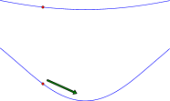
Figure 3: Illustration of the two misalignments at the electroweak (upper figure) and at the QCD phase transitions (lower figure) for a PQ-like axion (not to scale).

It is not difficult to show that the periodicity of the potential depends predominantly on $H_{0}^{4}$. This can be easily seen by analyzing the size of $\sigma_{H_{0}^{4}}$ and $\sigma_{H_{0}^{5}}$. In fact, expanding to first order in $a_{1}$ we get

$$\frac{1}{\sigma_{H_{0}^{4}}} =-\frac{4v_{1}v_{2}}{v_{2}\,\textrm{sgn}\,B_{S}\sqrt{v^{2}v_{S}^{2}+v_{1}^{2}v_{2}^{2}}}-\frac{8\sqrt{2}v_{1}^{2}v_{2}^{2}v_{S}^{4}\left[4v^{2}M_{St}^{2}+g_{B}^{2}B_{S}^{2}\left(v^{2}v_{S}^{2}+v_{1}^{2}v_{2}^{2}\right)\right]a_{1}}{a_{\lambda}M_{St}^{2}\left(v^{2}v_{S}^{2}+v_{1}^{2}v_{2}^{2}\right)^{5/2}\,\textrm{sgn}\,(B_{S})}+O\left(a_{1}^{2}\right)$$

$$\frac{1}{\sigma_{H_{0}^{5\prime}}} =-\frac{8\sqrt{2}v_{1}^{2}v_{2}^{2}v_{S}^{4}\left[4v^{2}M_{St}^{2}+g_{B}^{2}B_{S}^{2}\left(v^{2}v_{S}^{2}+v_{1}^{2}v_{2}^{2}\right)\right]a_{1}}{a_{\lambda}M_{St}^{2}\left(v^{2}v_{S}^{2}+v_{1}^{2}v_{2}^{2}\right)^{5/2}\,\textrm{sgn}\,B_{S}}+O\left(a_{1}^{2}\right).$$ (54)

with $a_{\lambda}$ being proportional to the SUSY breaking scale $M_{susy}$. A more careful look at the structure of these two scales shows that $\sigma_{H_{0}^{4}}\sim v_{S}$ ($v_{S}=400$ GeV in our case) while $\sigma_{H_{0}^{5}}\sim M_{susy}/\lambda_{eff}$. Clearly, $\sigma_{H_{0}^{5}}\gg\sigma_{H_{0}^{4}}$, but the dependence of the extra potential on $\chi$ is clearly affected by the different possible sizes of $\lambda_{eff}$. For an instanton generated potential ($\lambda_{eff}\sim\lambda_{inst}$) the direction of $\chi$ is essentially flat and $\sigma_{H_{0}^{5}}$ turns out to be very large. In turn, this implies that the dependence of the potential $V_{1}$ on $H_{0}^{5}$, which takes place exclusively through the exponential, is negligible, being essentially controlled by $H_{0}^{4}$ ($\overline{\theta}_{1}\sim H_{0}^{4}/v$) with

$$V_{1}\sim\lambda_{eff}v^{4}\cos(\overline{\theta}_{1}).$$ (55)

We may conclude, indeed, that in this case the effect of misalignment on $\chi$, generated at the electroweak scale, can be neglected. This feature is shown on the left panel of Fig. 4, where we plot $V^{\prime}(H_{0}^{4},\chi)$. It is immediately clear from these plots that for $\lambda_{eff}\sim\lambda_{inst}$ the only periodicity of the extra potential is in the variable $H_{0}^{4}$ (left panel), due to the flatness of the $H_{0}^{5}$ direction. For a more sizeable potential, with $\lambda_{eff}\sim 10^{-12}$, the curvature generated in $\chi$ is responsible for giving a mass to the axion in the MeV range (Fig. 4, right panel). This result is generic for all the terms.

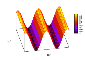
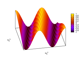
Figure 4: Shape of the extra potential $V^{\prime}$ at the electroweak scale in the CP-odd sector in the ($H_{0}^{4},\chi\equiv H_{0}^{5}$) plane. $\chi$ is an almost flat direction for a strength induced by the instanton vacuum at the electroweak scale (left panel) and acquires a curvature for an axion mass in the MeV region (curvature in the $\chi$ direction, right panel).

One can draw some conclusions regarding the role played by the exponential phase and compare the supersymmetric with the non-supersymmetric case. In the non-supersymmetric case the periodicity of the potential is controlled by the weak scale ($v$), and is expressed directly in terms of the physical component of $b$ (which is a real field). The size of the potential, in this case, is of order $\lambda_{eff}v^{4}$

$$V^{\prime}\sim\lambda_{eff}v^{4}\cos\left(\frac{\chi}{v}\right)$$ (56)

and therefore very small, while the periodicity shows that the amplitude of the axion field is $\chi\sim O(v)$. In the supersymmetric case, more generally, we obtain for a generic component $V_{i}$

$$V^{\prime}\sim\lambda M_{susy}^{4}\cos\left(\frac{H_{0}^{4}}{v_{S}}+\frac{\chi}{M_{susy}/\lambda_{eff}}\right)$$ (57)

from which it is clear that the curvature in the axion field is controlled by the parameter $\lambda_{eff}$. In the supersymmetric case we can think of the periodicity in Eq. (57) as essentially controlled by the massive CP-odd Higgs $H_{0}^{4}$, with a period which is $O(\pi v_{S})$, with superimposed a second periodicity of $O(\pi M_{susy}/\lambda_{eff})$ (with $M_{susy}/\lambda_{eff}\gg v_{S}$) in the perpendicular direction ($\chi$). We conclude that the actual structure of the complete ($V+V^{\prime}$) potential indeed guarantees the presence in the spectrum of a physical and light pseudoscalar field. This analysis holds, in principle, for an axion of any mass, although we do not explicitly study an axion whose mass goes beyond the MeV region. To have an axion which is long-lived, the true discriminant of our study is the axion mass, and for this reason we are going to present a study of the decay rates of this particle keeping the mass as a free parameter varying in the milli-eV - MeV interval.

6 Decay of a gauged supersymmetric axion

In this section we compute the decay rate of the axion of the supersymmetric model into two-photons, mediated both by the direct PQ interaction and by the fermion loop, which are shown in Fig. 5, keeping the axion mass as a free parameter.

+

Figure 5: Contributions to the axi-Higgs decay $\chi\,\rightarrow\gamma\gamma$.

Denoting with $N_{c}(f)$ the color factor for a fermion specie, and introducing the function $\tau_{f}\,\eta(\tau_{f})$, a function of the mass of the fermions circulating in the loop with

$$\tau=4m_{f}^{2}/m_{\chi}^{2}\hskip 28.45274pt\eta(\tau)=\arctan^{2}\frac{1}{\sqrt{-\rho_{f\chi}^{2}}}\hskip 28.45274pt\rho_{f\chi}=\sqrt{1-\left(\frac{2m_{f}}{m_{\chi}}\right)^{2}},$$ (58)

the WZ interaction in Fig. 5 is given by

$${\mathcal{M}}^{\mu\nu}_{WZ}(\chi\rightarrow\gamma\gamma)=4g^{\chi}_{\gamma\gamma}\varepsilon[\mu,\nu,k_{1},k_{2}],$$ (59)

where $g^{\chi}_{\gamma\gamma}$ is the coupling, defined via the relations

$$g^{\chi}_{\gamma\gamma}=-\frac{g_{B}B_{S}\left(4c_{Y}g_{2}^{2}+c_{W}g_{Y}^{2}\right)}{16g^{2}M_{St}}\sqrt{\frac{v^{2}v_{S}^{2}+v_{1}^{2}v_{2}^{2}}{4M_{St}^{2}v^{2}+g_{B}^{2}B_{S}^{2}\left(v^{2}v_{S}^{2}+v_{1}^{2}v_{2}^{2}\right)}}$$ (60)

obtained from the rotation of the WZ vertices on the physical basis (we will comment in more detail on the size of this coupling in the next section). The massless contribution to the decay rate coming from the WZ counterterm $\chi F_{\gamma}F_{\gamma}$ is given by

$$\Gamma_{WZ}(\chi\rightarrow\gamma\gamma)=\frac{m^{3}_{\chi}}{4\pi}(g^{\chi}_{\gamma\gamma})^{2}.$$ (61)

Combining also in this case the tree level decay with the 1-loop amplitude, we obtain for $\chi\rightarrow\gamma\gamma$ the amplitude

$${\mathcal{M}}^{\mu\nu}(\chi\rightarrow\gamma\gamma)={\mathcal{M}}^{\mu\nu}_{WZ}+{\mathcal{M}}^{\mu\nu}_{f}.$$ (62)

The second amplitude in Fig. 5 is mediated by the triangle loops and is given by the expression

$${\mathcal{M}}^{\mu\nu}_{f}(\chi\rightarrow\gamma\gamma)=\sum_{f}N_{c}(f)\,iC_{0}(m^{2}_{\chi},m_{f})c^{\chi,f}_{\gamma\gamma}\varepsilon[\mu,\nu,k_{1},k_{2}]\hskip 14.22636ptf=\{q_{u},q_{d},\nu_{l},l,\chi_{1}^{\pm},\chi_{2}^{\pm}\}$$ (63)

where $N_{c}(f)$ is the color factor for the fermions. In the domain $0<m_{\chi}<2m_{f}$, which is the relevant domain for our study, being the axion very light, the pseudoscalar triangle when both photons are on mass-shell is given by the expression

$$C_{0}(m^{2}_{\chi},m_{f})=-\frac{m_{f}}{\pi^{2}m_{\chi}^{2}}\arctan^{2}\left(\left(\frac{4m_{f}^{2}}{m_{\chi}^{2}}-1\right)^{-1/2}\right)=-\frac{m_{f}}{\pi^{2}m_{\chi}^{2}}\eta(\tau)$$ (64)

The coefficient $c^{\chi,f}_{\gamma\gamma}$ is the factor for the vertex between the axi-Higgs and the fermion current. The expressions of these factors are

$$c^{\chi,q_{u}} =-\frac{i\,\sqrt{2}\,y_{u}\,M_{St}\,v_{1}^{2}\,v_{2}}{\sqrt{(v^{2}v_{S}^{2}+v_{1}^{2}v_{2}^{2})\left[4M_{St}^{2}v^{2}+g_{B}B_{S}(v^{2}v_{S}^{2}+v_{1}^{2}v_{2}^{2})\right]}},$$

$$c^{\chi,q_{d}} =-\frac{v_{2}\,y_{d}}{v_{1}\,y_{u}}\,c^{\chi,q_{u}},$$

$$c^{\chi,l} =\frac{y_{e}}{y_{d}}\,c^{\chi,q_{d}}.$$ (65)

We obtain the following expression for the decay amplitude

$$\Gamma_{\chi}\equiv\Gamma(\chi\rightarrow\gamma\gamma)= \frac{m^{3}_{\chi}}{32\pi}\left\{8(g^{\chi}_{\gamma\gamma})^{2}+\frac{1}{2}\left|\sum_{f}N_{c}(f)i\frac{\tau_{f}\leavevmode\nobreak\ \eta(\tau_{f})}{4\pi^{2}m_{f}}e^{2}Q_{f}^{2}c^{\chi,f}\right|^{2}\right.$$

$$\left.\qquad\quad+4g^{\chi}_{\gamma\gamma}\sum_{f}N_{c}(f)i\frac{\tau_{f}\leavevmode\nobreak\ \eta(\tau_{f})}{4\pi^{2}m_{f}}e^{2}Q_{f}^{2}c^{\chi,f}\right\},$$ (66)

where the three terms correspond, respectively, to the point-like WZ term, to the 1-loop contribution and to their interference.

Notice that in the expression of this decay rate both the direct ($\sim{(g^{\chi}_{\gamma\gamma}})^{2}$) and the interference ($\sim g^{\chi}_{\gamma\gamma}$) contributions are suppressed as inverse powers of the Stückelberg mass, here taken to be equal to 1 TeV. We have chosen $v$ as the SM electroweak vev, for $v_{S}$ we have chosen the value of $500\,\textrm{GeV}$. In order to have an acceptable Higgs spectrum, the Yukawa couplings have been set to give the right fermion masses of the Standard Model, while for $g_{B}$ and $B_{S}$ we have chosen $g_{B}=0.1$ and $B_{S}=4$.

We show in Figs. 6 and 7 results obtained from the numerical evaluation of the decay amplitude as a function of the mass of the axion $m_{\chi}$, which clearly indicates that the decay rates are very small for a milli-eV particle, although larger than those of the PQ case [30]. We conclude that a PQ-like axion is indeed long-lived also in these models and as such could, in principle, contribute to the relic densities of dark matter. For an axion with a mass in the MeV region, instead, the particle is not stable and as such would decay rather quickly. The decay, in this case, is fast enough $(\tau\lesssim 10^{-3}$ sec) and does not interfere with the nucleosynthesis.

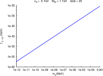
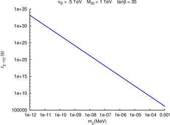
Figure 6: Decay amplitude (left panel) and mean lifetime (right panel) for $\chi\rightarrow\gamma\gamma$ as a function of the axi-Higgs mass.

7 Cold dark matter by misalignment of the axion field

In the case of a long-lived axion, the generation of relic densities of axion dark matter, in this model, involves two (sequential) misalignments, generated, as we have already discussed, the first at the electroweak scale, and the second at the QCD phase transition. The presence of two misalignments at two separate scales, as discussed in [30], is typical of axions which show interactions both with the weak and with the strong sectors, due to the presence of mixed anomalies. This point has been addressed in detail within a non-supersymmetric model, but in a supersymmetric scenario the physical picture remains the same.

In the PQ-like case, at the first misalignment, taking place at the electroweak scale, the physical axion is singled out as a component of $\textrm{Im}\,b$, with a mass which is practically zero, due to the small value of the curvature induced by the potential generated by electroweak instantons (Fig. 3, top) given in Eq. (44). In the case of a very small extra potential ($\lambda_{eff}\sim\lambda_{inst}$) it is the second misalignment to be responsible for generating an axion mass. At the second misalignment, taking place at the QCD phase transition, the mass of this pseudo Nambu-Goldstone mode is redefined from zero to a small but more significant value ($\sim 10^{-3}$ eV) induced by the QCD instantons ((Fig. 3, bottom). The final value of the mass is determined in terms of the hadronic scale $\Lambda_{QCD}$ and of a second intermediate scale, $M_{St}^{2}/v$, which replaces $f_{a}$ in all of the expressions usually quoted in the literature and held valid for PQ axions, as we are now going to clarify.

• MeV axion

An MeV axion is allowed only if the extra potential (the misalignment) is assumed to be generated at a scale different from the electroweak phase transition, say at an earlier time. This misalignment, in fact, should be unrelated to the (quasi-periodic) corrections induced at the electroweak time, as shown in Fig. 4, being the latter of very small size. However, such an axion would not be long lived. One can easily realize that in this scenario, due to the sizeable value of $m_{\chi}$, there is an overlap between the period of coherent oscillations at the QCD hadron transition and the typical lifetime at which the axion decays. This can be trivially checked by comparing the QCD time, defined as the inverse Hubble rate at the temperature of confinement ($H(T_{QCD})\sim 10^{-11}$ eV, $T_{QCD}\sim 200$ MeV) $t_{QCD}\sim 10^{-4}$ sec with the axion lifetime in this typical mass range.

• PQ-like axion

For a PQ-like axion the effective scale ($M_{St}^{2}/v$) is the result of the product of two factors: a first factor due to the rotation matrix of the Stückelberg field $\textrm{Im}\,b$ onto $\chi$ - which is proportional to $v/M$ - times a second factor ($1/M_{St}$) which is inherited from the original $\textrm{Im}\,b/M_{St}\,F\tilde{F}$ (WZ) counterterm. Specifically, starting from Eq. (43), the size of the projection of $\textrm{Im}\,b$ into $\chi$ is given by

$$\frac{1}{N_{\chi}}B_{S}\,g_{B}(v^{2}v_{S}^{2}+v_{1}^{2}v_{2}^{2})\sim v/M_{St}$$ (67)

and hence a typical PQ interaction term involving the Stückelberg field $b$ becomes

$$\frac{\textrm{Im}\,b}{M_{St}}FF^{\prime}\to\frac{\chi}{M_{St}^{2}/v}FF^{\prime}.$$ (68)

The physical state with a $b$ component (i.e. $\chi$) acquires an interaction to $F\tilde{F}$ which is suppressed by the scale $M_{St}^{2}/v$.

Having identified this scale, if we neglect the axion mass generated by $V^{\prime}$ (Eq. 44) at the electroweak scale, the final mass of the physical axion induced at the QCD scale is controlled by the ratio $m_{\chi}\sim\Lambda_{QCD}^{2}v/M_{St}^{2}$, where the angle of misalignment is given by $\theta^{\prime}=\chi v/M_{St}^{2}$.

Coming to the value of the abundances for a PQ-like axion - defined as the number density to entropy ratio $Y=n_{\chi}/s$ - these can be computed in terms of the relevant suppression scale appearing in the $\chi F\tilde{F}$ interaction. We have expanded on the structure of the computation in Appendix C. If we indicate with $\theta^{\prime}(T_{i})$ the angle of misalignment at the QCD hadron transition and with $T_{i}$ the initial temperature at the beginning of the oscillations, the expression of the abundances takes the form

$$Y_{\chi}(T_{i})=\left(\frac{v}{M_{St}}\right)\frac{45M_{St}^{2}\left(\theta^{\prime}(T_{i})\right)^{2}}{2\sqrt{5\pi g_{*,T}}T_{i}M_{P}},$$ (69)

which depends linearly on $M_{St}$. As we have already mentioned, the computation of the relic densities for a non-thermal population follows rather closely the approach outlined in the non-supersymmetric case. For instance, a rather large value of $M_{St}$, of the order of $10^{7}$ GeV [30], determines a sizeable contribution of the gauged axion to the relic densities of cold dark matter. These, in turn, follow rather closely the behaviour expected in the case of the PQ axion. In practice, to obtain a sizeable non-thermal populations of gauged axions, $M_{St}$ should be such that $M_{St}^{2}/v\sim f_{a}$, with $f_{a}$ the usual estimated size of the PQ axion decay constant. This allows a sizeable contribution of $\chi$ to the relic density of cold dark matter, with a partial contribution to $\Omega$ ($\Omega_{\chi}h^{2}\sim 0.1$) in close analogy to what expected in the case of the PQ axion. These considerations, which are in close relations with what found in the non-supersymmetric construction [30], in this case will be subject to the constraints coming from the neutralino sector and its abundances derived from WMAP. We will come back to this point after presenting the results of our simulations in the next sections.

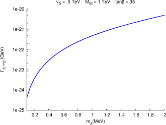
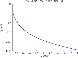
Figure 7: Decay amplitude and mean lifetime for $\chi\rightarrow\gamma\gamma$ as a function of the axi-Higgs mass for an axion whose mass in the MeV range.

8 The neutralino sector

The neutralino sector is constructed from the eigenstates of the space spanned by the neutral fields ($i\lambda_{W^{3}}$, $i\lambda_{Y}$, $i\lambda_{B}$, $\tilde{H_{1}^{1}}$, $\tilde{H_{2}^{2}}$, $\tilde{S}$, $\psi_{\bf b}$), which involve the three neutral gauginos, the two Higgsinos, the singlino (the fermion component of the singlet superfield) and the axino component of the Stückelberg supermultiplet. We denote with $M_{\chi_{0}}$ the corresponding mass matrix and we list its components in the appendix. The neutralino eigenstates of this mass matrix are labelled as $\tilde{\chi}_{i}^{0}$ ($i=0,\dots,6$) and can be expressed in the basis $\{i\lambda_{W_{3}},i\lambda_{Y},i\lambda_{B},\tilde{H}^{1}_{1},\tilde{H}^{2}_{2},\tilde{S},\psi_{\bf b}\}$

$$\tilde{\chi}^{0}_{i}=a_{i1}\,i\lambda_{W_{3}}+a_{i2}\,i\lambda_{Y}+a_{i3}\,i\lambda_{B}+a_{i4}\,\tilde{H}^{1}_{1}+a_{i5}\,\tilde{H}^{2}_{2}+a_{i6}\,\tilde{S}+a_{i7}\,\psi_{\bf b}.$$ (70)

The neutralino mass eigenstates are ordered in mass and the lightest eigenstate corresponds to $i=0$. We indicate with $O^{\,{\chi}^{0}}$ the rotation matrix that diagonalizes the neutralino mass matrix. In order to perform a numerical analysis of the model we need to fix some of the parameters, first of all requiring consistency of their choice with the masses of the Standard Model particles. For this purpose, the Higgs vev’s $v_{1}$ and $v_{2}$ have been constrained in order to generate the correct mass values of the $W^{\pm}$, which depends on $v^{2}=v_{1}^{2}+v_{2}^{2}$, and of the $Z$ gauge boson.

The Yukawa couplings have been fixed in order to give the correct masses of the SM fermions. The choice of $v_{S}$ and of the parameter $\lambda$ in the trilinear term $\lambda SH_{1}\cdot H_{2}$ in the scalar potential has been made in order to obtain mass values in the Higgs sector in agreement with the limits from direct searches (with $\lambda\sim O(1)$). For this reason we have selected the value $\lambda=0.5$ and the assignment $B_{H_{1}}=-1,B_{S}=3$ for the $U(1)_{B}$ charges of the Higgs and the singlet; $B_{Q}=2$ for the quark doublet, and $B_{L}=1$ for the lepton doublet. The gauge mass terms parameters have been selected according to the relation

$$M_{Y}:M_{W}:M_{G}=1:2:6,$$ (71)

coming from the unification condition for the gaugino masses. As a further simplification, the sfermion mass parameters $M_{L}$, $M_{Q}$, $m_{R}$, $m_{D}$ and $m_{U}$ have been set to a unique value $M_{0}$. We have also chosen a common value $a_{0}$ for the trilinear couplings $a_{e}$,$a_{d}$ and $a_{u}$. With these choices, besides $\tan\beta$, the only other free parameters left are the Stückelberg mass $M_{St}$, the gaugino mass term for $\lambda_{B}$, denoted by $M_{B}$, and the axino mass term, $M_{b}$. Our choices are the following

$$M_{Y}=500\textrm{GeV}\hskip 14.22636ptM_{YB}=1\,\textrm{TeV}\hskip 14.22636ptM_{W}=1\,\textrm{TeV}\hskip 14.22636ptM_{G}=3\,\textrm{TeV}$$

$$M_{L}=M_{Q}=m_{R}=m_{D}=m_{U}=M_{0}=1\,\textrm{TeV}$$

$$a_{e}=a_{d}=a_{u}=a_{0}=1\,\textrm{TeV}$$

$$a_{\lambda}=-100\,\textrm{GeV},$$ (72)

where with $M_{L}$ and $M_{Q}$ we have denoted the scalar mass terms for the sleptons and the squarks, assumed to be equal for all the 3 generations. We have also chosen

$$M_{B}=M_{b}=1\,\textrm{TeV}$$ (73)

with a coupling constant $g_{B}$ of the anomalous $U(1)$ of $0.4$. From previous investigations such values of the anomalous coupling are known to be compatible with LEP data at the $Z$ resonance [43, 44]. In particular, the mass of the extra $Z^{\prime}$ ($M_{Z^{\prime}}$), which in our case is of the order of the Stückelberg mass, $M_{Z^{\prime}}\sim M_{St}$ [43], due to the region of variability of $M_{St}$ that we investigate in our simulations, obviously satisfies the current LHC constraints at 95% CL ( $>1140$ GeV) from CMS [45] and from ATLAS ($>$ 1.83 TeV) [46] on the absence of a resonance in the dilepton channel at 7 TeV for an extra Z prime with Standard-Model like couplings. This parameter choice is our benchmark, which is compatible with all the SM requirements on the spectrum of the known particles. It involves SUSY breaking scales in a kinematical range which is under investigation at the LHC. We also assume a value $v_{b}=20$ GeV for the vev of the saxion field Re$b$.

The most significant parameters in the relic density calculation are $M_{St}$ and the Higgs vev ratio $\tan\beta$. Concerning the Stückelberg mass, its value has been chosen to be varied in two different regions, $2-10$ TeV and $11-25$ TeV. In both regions we will consider different values of $\tan\beta$.

9 Neutralino relic densities and cosmological bounds

As it is well known, the evaluation of the relic densities requires the calculation of a great number of thermally averaged cross sections, given the number of particles which are present. Before coming to the discussion of the results of this very involved analysis, which is summarized just in some simple plots of the relic densities of the lightest neutralino - as a function both of $M_{St}$ and $\tan\beta$, - we present a general description of the structure of the interactions in the model. We also list the 2-to-2 processes that have been considered in the coupled Boltzmann equations.

We start from the action involving the physical axion ($H_{0}^{5}$) and its interactions with the various sectors. These involve, typically, interactions with the Higgs sector via bilinear vertices (proportional to $R^{H_{0}^{5}\,HH}$), and trilinear ones (proportional to $R^{H_{0}^{5}\,HHH}$) in $H$, with $H$ denoting generically CP-even and CP-odd Higgs eigenstates. Other interactions in the same component of the Lagrangian involve axion-neutralino terms ($R^{H_{0}^{5}\,\chi_{i}^{0}\chi_{j}^{0}}$) plus axion-charginos ($R^{H_{0}^{5}\,\chi_{i}^{\pm}\chi_{j}^{\mp}}$). Other terms are those involving interactions of the axion with the sleptons $(R^{H_{0}^{5}\tilde{l}_{i}^{\,\dagger}\tilde{l}_{j}})$ and the squarks $(R^{H_{0}^{5}\tilde{q}_{i}^{\dagger}\tilde{q}_{j}})$; vertices involving gauge bosons (for instance $R^{H_{0}^{5}A\chi^{\pm}_{i}\chi^{\mp}_{j}}$, with a photon $A$ and two charginos) and quartic contributions with 2, 3 and 4 axion lines. The Lagrangian describing all the tree-level interactions involving the axion is

$${\cal L}_{H_{0}^{5}-int}= R^{H_{0}^{5}H_{0}^{4}H_{0}^{i}}H_{0}^{5}H_{0}^{4}H_{0}^{i}+R^{H_{0}^{5\,\,2}H_{0}^{i}}\left(H_{0}^{5}\right)^{2}H_{0}^{i}+R^{H_{0}^{5}H_{0}^{4}H_{0}^{i}H_{0}^{j}}H_{0}^{5}H_{0}^{4}H_{0}^{i}H_{0}^{j}+R^{H_{0}^{5\,2}H_{0}^{i}H_{0}^{j}}\left(H_{0}^{5}\right)^{2}H_{0}^{i}H_{0}^{j}+$$

$$R^{H_{0}^{5}H_{0}^{4\,3}}H_{0}^{5}H_{0}^{4\,3}+R^{H_{0}^{5\,2}H_{0}^{4\,2}}\left(H_{0}^{5}\right)^{2}\left(H_{0}^{4}\right)^{2}+R^{H_{0}^{5\,3}H_{0}^{4}}\left(H_{0}^{5}\right)^{3}H_{0}^{4}+R^{H_{0}^{5\,4}}\left(H_{0}^{5}\right)^{4}+$$

$$R^{H_{0}^{5}\chi^{0}_{i}\chi^{0}_{j}}H_{0}^{5}\chi^{0}_{i}\chi^{0}_{j}+R^{H_{0}^{5}\chi^{\pm}_{i}\chi^{\mp}_{j}}H_{0}^{5}\chi^{\pm}_{i}\chi^{\mp}_{j}+R^{H_{0}^{5}\tilde{l}_{i}\tilde{l}_{j}}H_{0}^{5}\tilde{l}_{i}^{\,\dagger}\tilde{l}_{j}+R^{H_{0}^{5}\tilde{q}_{i}\tilde{q}_{j}}H_{0}^{5}\tilde{q}_{i}^{\dagger}\tilde{q}_{j}+$$

$$R^{H_{0}^{5}A\chi^{\pm}_{i}\chi^{\mp}_{j}}H_{0}^{5}A^{\mu}\bar{\chi}^{\pm}_{i}\gamma_{\mu}\chi^{\mp}_{j}+R^{H_{0}^{5}Z\chi^{\pm}_{i}\chi^{\mp}_{j}}H_{0}^{5}Z^{\mu}\bar{\chi}^{\pm}_{i}\gamma_{\mu}\chi^{\mp}_{j}+R^{H_{0}^{5}Z^{\prime}\chi^{\pm}_{i}\chi^{\mp}_{j}}H_{0}^{5}Z^{\prime\mu}\bar{\chi}^{\pm}_{i}\gamma_{\mu}\chi^{\mp}_{j}+$$

$$R^{H_{0}^{5}W^{\mp}\chi^{\pm}_{i}\chi^{0}_{j}}H_{0}^{5}W^{\mp}_{\mu}\bar{\chi}^{0}_{j}\gamma^{\mu}\chi^{\mp}_{i}+R^{\chi^{0}_{i}\chi^{\pm}H^{\mp}H_{0}^{5}}\chi^{0}_{i}\chi^{\pm}_{j}H^{\mp}H_{0}^{5}+R^{\chi^{0}_{i}\chi^{0}_{j}H_{0}^{5}H_{0}^{4}}\chi^{0}_{i}\chi^{0}_{j}H_{0}^{5}H_{0}^{4}.$$ (74)

The explicit expressions of these vertices are rather involved and we omit them. Other interactions appearing in the interaction Lagrangian involve derivative couplings with the gauge bosons and the Higgses and they are given by

$${\cal L}_{H_{0}^{5}-int} =R^{H_{0}^{5}H^{\pm}W^{\mp}}H_{0}^{5}W_{\mu}^{\mp}\partial^{\mu}H^{\pm}+R^{H_{0}^{5}H_{0}^{i}A}H_{0}^{5}A_{\mu}\partial^{\mu}H_{0}^{i}+R^{H_{0}^{5}H_{0}^{i}Z}H_{0}^{5}Z_{\mu}\partial^{\mu}H_{0}^{i}+$$

$$R^{H_{0}^{5}H_{0}^{i}Z^{\prime}}H_{0}^{5}Z_{\mu}^{\prime}\partial^{\mu}H_{0}^{i}.$$ (75)

Similar interactions are also typical for $H_{0}^{4}$, the CP-odd Higgs. Some of the vertices are illustrated in Fig. 8.

Figure 8: Axi-Higgs ($H^{5}_{0}$) interactions. The double arrows denote Majorana particles (neutralinos).

Besides the interaction with the axi-Higgs, we have the following vertices involving neutralinos

$${\cal L}_{\chi_{0}-int} =R^{\chi^{0}_{i}\chi^{0}_{j}Z}Z^{\mu}\bar{\chi}^{0}_{i}\gamma_{\mu}\chi^{0}_{j}+R^{\chi^{0}_{i}\chi^{0}_{j}Z^{\prime}}Z^{\prime\mu}\bar{\chi}^{0}_{i}\gamma_{\mu}\chi^{0}_{j}+R^{\chi^{0}_{i}\chi^{\pm}_{j}W^{\mp}}W^{\mp}_{\mu}\bar{\chi}^{0}_{i}\gamma_{\mu}\chi^{\pm}_{j}+R^{\chi^{0}_{i}\chi^{\pm}_{j}H^{\mp}}H^{\mp}\chi^{0}_{i}\chi^{\pm}_{j}+$$

$$R^{\chi^{0}_{i}\chi^{0}_{j}H_{0}^{k}}H_{0}^{k}\chi^{0}_{j}\chi^{0}_{k}+R^{\chi^{0}_{i}f\tilde{f}}\chi^{0}_{i}f\tilde{f}_{1,2}+R^{\chi^{0}_{i}\chi^{\pm}_{j}\tilde{q}^{\dagger}\tilde{q}}\chi^{0}_{i}\chi^{\pm}_{j}\tilde{q}^{\dagger}_{k}\tilde{q}_{l}+R^{\chi^{0}_{i}\chi^{0}_{j}\tilde{f}^{\dagger}\tilde{f}}\chi^{0}_{i}\chi^{\pm}_{j}\tilde{f}^{\dagger}_{k}\tilde{f}_{l}+$$

$$R^{\chi^{0}_{i}\chi^{\pm}_{j}H^{\mp}H_{0}^{k}}\chi^{0}_{i}\chi^{\pm}_{j}H^{\mp}H_{0}^{k}+R^{\chi^{0}_{i}\chi^{0}_{j}H_{0}^{k}H_{0}^{l}}\chi^{0}_{i}\chi^{0}_{j}H_{0}^{k}H_{0}^{l}+R^{\chi^{0}_{i}\chi^{0}_{j}H^{\pm}H^{\mp}}\chi^{0}_{i}\chi^{0}_{j}H^{\pm}H^{\mp}.$$ (76)

Some of these vertices are illustrated in Fig. 9.

Figure 9: Neutralino interactions

The full lagrangian has been implemented using the FeynRules[47] package. The same package allows to generate the CalcHEP[48] model files which are needed by micrOMEGAs[49] for the calculation of the scattering cross section that are required in the relic density calculation.

With our choice for the parameters the lightest neutralino is the Lightest Supersymmetric Particle (LSP) and so it is the dark matter component in our simulations. The value of the neutralino mass in this case turns out to be around 23 GeV with a rather mild dependence on $\tan\beta$. For $\tan\beta$ varying between 5 and 25 the neutralino mass varies from 22.4 to 23.8 GeV.

We show in Tab. 1 a list of the most relevant 2-to-2 processes which are generated in the $s,t$ and $u$ channels having neutralinos in the initial state (in), while the possible final states are shown on the right-hand side of the same table (out).

in	s-channel	out
$\chi^{0}_{i}\,\chi^{0}_{j}$	$Z$,$Z^{\prime}$	$H^{\pm}H^{\mp}$,$H_{0}^{k}H_{0}^{4}$,$H_{0}^{k}H_{0}^{5}$,$Z/Z^{\prime}H_{0}^{k}$,$\bar{f}f$,$\tilde{f}^{\dagger}\tilde{f}$
	$H_{0}^{k}$	$H^{\pm}H^{\mp}$,$H_{0}^{l}H_{0}^{m}$,$H_{0}^{4}H_{0}^{4}$,$H_{0}^{4}H_{0}^{5}$,$H_{0}^{5}H_{0}^{5}$,$Z/Z^{\prime}H_{0}^{4}/H_{0}^{5}$,
		$W^{\pm}H^{\mp}$,$Z/Z^{\prime}Z/Z^{\prime}$,$W^{\pm}W^{\mp}$,$\bar{f}f$,$\tilde{f}^{\dagger}\tilde{f}$
	$H_{0}^{4},H_{0}^{5}$	$H_{0}^{k}H_{0}^{4}$,$H_{0}^{k}H_{0}^{5}$,$Z/Z^{\prime}H_{0}^{k}$,$W^{\pm}H^{\mp}$,$\bar{f}f$,$\tilde{f}^{\dagger}\tilde{f}$

in	t/u-channel	out
$\chi^{0}_{i}\,\chi^{0}_{j}$	$\chi^{0}_{k}$	$H_{0}^{l}H_{0}^{m}$,$H_{0}^{l}H_{0}^{4}/H_{0}^{5}$,$H_{0}^{4}/H_{0}^{5}H_{0}^{4}/H_{0}^{5}$,
		$Z/Z^{\prime}H_{0}^{l}/H_{0}^{4}/H_{0}^{5}$,$Z/Z^{\prime}Z/Z^{\prime}$
	$\chi^{\pm}_{k}$	$W^{\pm}/H^{\pm}W^{\mp}/H^{\mp}$
	$\tilde{f}$	$\bar{f}f$

Table 1: Tree level neutralino annihilation processes in the 3 kinematic channels

In Fig. 10 we show the results obtained for the lightest neutralino relic density with $M_{St}$ in the range $5-8$ TeV, $v_{S}=600$ GeV and a varying $\tan\beta$. The values of $v_{S}$, $\tan\beta$ and $M_{St}$ for which we plot the result coming from the relic density calculation are those that give also acceptable mass values for the whole spectrum, in particular for the neutral Higgs ($\sim 124-126$ GeV) [50, 51]. The horizontal bar represents the experimental value for the physical dark matter density measured by WMAP, $\Omega h^{2}=.1123\pm.0035$[52].

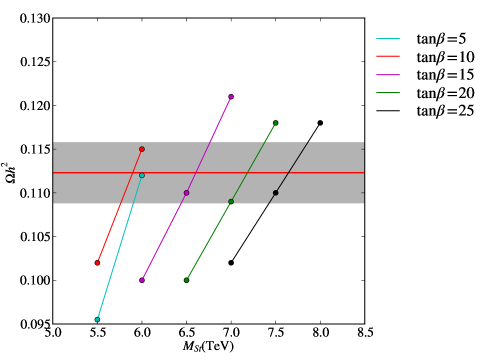
Figure 10: Relic density of the lightest neutralino as a function of the Stückelberg mass in the region $5-8.5$ TeV for different values of the Higgs vev ratio $\tan\beta$

In Fig. 11 we show the analogous results obtained in the range $11-24$ TeV with $v_{S}=1.2$ TeV and varying $\tan\beta$. Once again these values are such that we obtain acceptable values for the masses of all the particles in the model. One can immediately notice that for a fixed value of $\tan\beta$ as we increase $M_{St}$, the relic densities grow and tend to violate the WMAP bound. This trend has been found over a sizable range of variability of $\tan\beta$ and is a central feature of the model. It is then obvious, from the same figures, that it is possible to raise the Stuckelberg mass and stay below the bound if, at the same time, we increase $\tan\beta$.

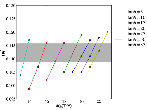
Figure 11: Relic density of the lightest neutralino as a function of the Stückelberg mass in the region $2-24$ TeV for different values of the Higgs vev ratio $\tan\beta$

10 Summary: windows on the axion mass

At this point, before coming to our conclusions, we can try to gather all the information that we have obtained so far in the previous sections, summarizing the basic properties of axions in these types of models.

• The milli-eV (PQ-like) axion

One possibility that we have explored in this work is that $V^{\prime}$, the extra potential which is periodic in the axion field, may be generated around the TeV scale or at the electroweak phase transition. The actual strength of the potential, remains, in our construction, undetermined and the physical features of the axion (primarily its mass), depend upon this parameter. We have tried to describe the various possibilities, in this respect, and the essential features for each choice for the value of the mass. In particular, if the extra potential is generated by non-perturbative effects at the electroweak phase transition, then the mass of the axion is tiny and the true mechanism of misalignment which determines its mass takes place at a second stage, at the QCD phase transition. In this case the physical axion of the model would be no much different from an ordinary PQ axion and would be rather long-lived. At the same time, its abundances are fixed by the possible value of the scale $M_{St}^{2}/v$, which should be rather large ($\sim 10^{10}-10^{12}$ GeV), of the same order of $f_{a}$ in typical axion models, to be a significant component of cold dark matter. In the region that we have analyzed numerically, with $M_{St}$ around the 2-20 TeV’s, the contribution to dark matter from misalignment of the axion field, in this case, should be small.

A second important constraint on this particle, in this mass range, comes from direct axion searches, which also requires the interaction of the axions with the gauge fields (in particular the photon) to be suppressed by a large $f_{a}$. For this reason, with $M_{St}$ in the TeV region, these simulations indicate that an axion of this mass, in fact, can be excluded by typical searches with detectors of Sikivie type. The reason is rather obvious, since axions in the milli-eV mass range could be copiously produced at the center of the sun and probably should have been seen by now in ground based detectors (helioscopes), such as CAST [53]. We recall that one of the goals of searches with helioscopes is to set a lower bound on the suppression scale $f_{a}$ of the axion-photon vertex, which is currently experimentally constrained, as we have already mentioned, to be rather large.

• The meV axion

A second possibility that we have investigated is that the extra potential appearing in the CP-odd sector is unrelated to instanton corrections in the electroweak vacuum. In this case the mass of the axion remains a free parameter. The range that we have explored in this second case involves an axion mass in the MeV region, discussing the several constraints that emerge from the model. In this case the axion is, in general, not long-lived and as such is not a component of dark matter. On the other hand, the constraints from CAST can be avoided, since the particle would not be produced by ordinary thermal mechanisms at the center of the sun, where the temperature is about 1.7 keV, being its mass above the keV range. Obviously, in this case other constraints emerge from nucleosynthesis requirements, since a particle in this mass range has to decay fast enough in order not to generate a late entropy release at nucleosynthesis time. We have seen that an axion in the MeV range is consistent with these two requirements. An axion of this type could be searched for at colliders, and in this respect the analysis of its possible detection at the LHC would follow quite closely the patterns described by two of us in [41]. As in this previous (non-supersymmetric) study, where the axion is Higgs-like (of a mass in the GeV region) typical channels where to look for this particle would be a) the associated production of an axion and a direct photon; b) the multi-axion production channel, and c) the associated production of one axion and other Higgses of the CP-even sector. The modifications, compared to that previous study, would now involve 1) the lower value of the mass of the axion (MeV rather than GeV); 2) the presence of extra supersymmetric interactions.

10.1 Comments

One important comment concerns the connection between these class of models and their completion theories such as string theory, which lay at their foundation. In our study we have selected a scenario characterized by low energy supersymmetry, with a phenomenological analysis that is essentially connected with the TeV scale and above. This is the scale which is likely to be scanned in the near future by several experiments, including the LHC, and for this reason we have directed out numerical studies in this direction. There is, however, a second it involves a value of $M_{St}$ which is very large and close to the Planck scale. In this second case the model predicts, obviously, a decoupling of the anomalous symmetry, leaving at low energy a scenario which is essentially the same of the MSSM, since the extra $Z$ prime, which is part of the spectrum, is extremely heavy. This would obviously imply a decoupling both of the anomalous gauge boson and of the anomalous trilinear interactions which are associated with it. A physical axion could, however, survive this limit, if the scale of the extra potential is also of the order of $M_{St}$, but its interaction with ordinary matter would be extremely suppressed by the same scale.

11 Conclusions

The investigation of the phenomenological role played by models containing anomalous gauge interactions from abelian extensions of the Standard Model, we believe that will receive further attention in the future. These studies can be motivated within several scenarios, including string and supergravity theories, in which gauged axionic symmetries are introduced for anomaly cancellation. In turn, these modified mechanisms of cancellation of the anomalies, which involve an anomalous fermion spectrum and an axion, are essentially connected with the UV completion of these field theories, which in a string framework is realized by the Green-Schwarz mechanism.

The model that we have investigated (the USSM-A) summarizes the most salient physical features of these types of constructions, where a Stückelberg supermultiplet is associated to an anomalous abelian structure in order to restore the gauge invariance of the anomalous effective action. In this work we have tried to characterize in detail some among the main phenomenological implications of these models, which are particularly interesting for cosmology. The physical axion of this construction, or gauged axion, emerges as a component of the Stückelberg field $\textrm{Im}\,b$. We have pointed out that the mechanism of sequential misalignment, formerly discussed in the non-supersymmetric case [30], finds a natural application also in the presence of supersymmetry, with minor modifications.

One relevant feature of these models, already noticed in [30], is that their axions do not contribute to the isocurvature perturbations of the early universe, being gauge degrees of freedom at the scale of inflation.

We have followed a specific pattern in order to come out with specific results in these types of models, using for this purpose a particular superpotential (the USSM superpotential), whose essential features, however, may well be generic.

We have presented an accurate study of the neutralino relic densities, showing that the Stückelberg mass value is constrained by the requirement of a consistent mass spectrum, with values for the lightest CP-even Higgs larger than the current LHC limits ( $>$ 120 GeV)

and by the experimental value for the dark matter abundance from WMAP [52]. Thus, in these models, the allowed value of the Stückelberg scale is positively correlated with the value of $\tan\beta$. As it grows, $\tan\beta$ has also to grow (for a fixed value of the vev of the singlet $v_{S}$) in order to preserve the WMAP bound. In particular $M_{St}$ and $v_{S}$ are positively correlated. This correlation is necessary in order to obtain values of the neutralino mass which allow to satisfy the same bounds, which in our case is around 20 GeV.

We have seen that with a Stückelberg mass in the TeV range the non-thermal population of axions does not contribute significantly to the dark matter densities if these axions are PQ-like. These types of constraints, obviously, are typical of supersymmetric constructions and are avoided in a non-supersymmetric context. In this second case, as discussed in [30], a Stückelberg scale around $10^{7}$ GeV is sufficient to revert this trend.

We have also pointed out that gauged axions in the milli-eV mass range are probably difficult to reconcile with current bounds from direct searches, while the case for detecting MeV or heavier axions, in these types of models, remains a wide open possibility. In this second case, cascade decays of these light particles and their associated production with photons should be seen as their possible event signatures at the LHC.

Acknowledgements

We thank Nikos Irges, George Lazarides and Antonio Racioppi for discussions. This work is supported in part by the European Union through the Marie Curie Research and Training Network UniverseNet (MRTN-CT-2006-035863).

Appendix A General Features of the Model

In this appendix we summarize some of the basic features of the USSM-A. The gauge structure of the model is of the form $SU(3)_{c}\times SU(2)\times U(1)_{Y}\times U(1)_{B}$, where $B$ is the anomalous gauge boson, and with a matter content given by the usual generations of the Standard Model (SM). In all the Lagrangians below we implicitly sum over the three fermion generations. A list of the fundamental superfields and charge assignments is summarized in Tab. 2. The Lagrangian can be expressed as

$${\cal L}_{USSM-A}={\cal L}_{USSM}+{\cal L}_{KM}+{\cal L}_{FI}+{\cal L}_{axion}$$ (77)

where the Lagrangian of the USSM (${\cal L}_{USSM}$) has been modified by the addition of ${\cal L}_{axion}$ to compensate for the anomalous variation of the corresponding effective action due to the anomalous charge assignments. The former is given by

$${\cal L}_{USSM}={\cal L}_{lep}+{\cal L}_{quark}+{\cal L}_{Higgs}+{\cal L}_{gauge}+{\cal L}_{SMT}+{\cal L}_{GMT}$$ (78)

with contributions from the leptons, quarks and Higgs plus gauge kinetic terms. The matter contributions from leptons and quarks

$${\cal L}_{lep}=\int{d^{4}\theta\left[\hat{L}^{\dagger}e^{2g_{2}\hat{W}+g_{Y}\hat{Y}+g_{B}\hat{B}}\hat{L}+\hat{R}^{\dagger}e^{2g_{2}\hat{W}+g_{Y}\hat{Y}+g_{B}\hat{B}}\hat{R}\right]}$$ (79)

$${\cal L}_{quark}=\int d^{4}\theta\left[\hat{Q}^{\dagger}e^{2g_{s}\hat{G}+2g_{2}\hat{W}+g_{Y}\hat{Y}+g_{B}\hat{B}}\hat{Q}+\hat{U}_{R}^{\dagger}e^{2g_{s}\hat{G}+g_{Y}\hat{Y}+g_{B}\hat{B}}\hat{U}_{R}+\hat{D}_{R}^{\dagger}e^{2g_{s}\hat{G}+g_{Y}\hat{Y}+g_{B}\hat{B}}\hat{D}_{R}\right]$$ (80)

are accompanied by a sector which involves two Higgs $SU(2)$ doublet superfields, $\hat{H}_{1}$ and $\hat{H}_{2}$, and one singlet $\hat{S}$

$${\cal L}_{Higgs}=\int{d^{4}\theta\left[\hat{H}_{1}^{\dagger}e^{2g_{2}\hat{W}+g_{Y}\hat{Y}+g_{B}\hat{B}}\hat{H}_{1}+\hat{H}_{2}^{\dagger}e^{2g_{2}\hat{W}+g_{Y}\hat{Y}+g_{B}\hat{B}}\hat{H}_{2}+\hat{S}^{\dagger}e^{g_{B}\hat{B}}\hat{S}+{\cal W}\delta^{2}(\bar{\theta})+\bar{{\cal W}}\delta^{2}(\theta)\right]}$$ (81)

with the superpotential chosen of the form

$${\cal W}=\lambda\hat{S}\hat{H}_{1}\cdot\hat{H}_{2}+y_{e}\hat{H}_{1}\cdot\hat{L}\hat{R}+y_{d}\hat{H}_{1}\cdot\hat{Q}\hat{D}_{R}+y_{u}\hat{H}_{2}\cdot\hat{Q}\hat{U}_{R}.$$ (82)

This superpotential, as shown in [34, 35], allows a physical axion in the spectrum. The gauge content plus the soft breaking terms in the form of scalar mass terms (SMT) are identical to those of the USSM

$${\cal L}_{gauge}=\frac{1}{4}\int{d^{4}\theta\left[{\cal G}^{\alpha}{\cal G}_{\alpha}+W^{\alpha}W_{\alpha}+W^{Y\alpha}W^{Y}_{\alpha}+W^{B\alpha}W^{B}_{\alpha}\right]\delta^{2}(\bar{\theta})+h.c.}$$

$${\cal L}_{SMT}=-\int d^{4}\theta\,\delta^{4}(\theta,\bar{\theta})\,[M^{2}_{L}\hat{L}^{\dagger}\hat{L}+m^{2}_{R}\hat{R}^{\dagger}\hat{R}+M^{2}_{Q}\hat{Q}^{\dagger}\hat{Q}+m^{2}_{U}\hat{U}_{R}^{\dagger}\hat{U}_{R}+m^{2}_{D}\hat{D}_{R}^{\dagger}\hat{D}_{R}$$

$$\hskip 71.13188pt+m_{1}^{2}\hat{H}_{1}^{\dagger}\hat{H}_{1}+m_{2}^{2}\hat{H}_{2}^{\dagger}\hat{H}_{2}+m_{S}^{2}\hat{S}^{\dagger}\hat{S}+(a_{\lambda}\hat{S}\hat{H}_{1}\cdot\hat{H}_{2}+h.c.)+(a_{e}\hat{H}_{1}\cdot\hat{L}\hat{R}+h.c.)$$

$$\hskip 71.13188pt+(a_{d}\hat{H}_{1}\cdot\hat{Q}\hat{D}_{R}+h.c.)+(a_{u}\hat{H}_{2}\cdot\hat{Q}\hat{U}_{R}+h.c.)].$$ (83)

As usual, $M_{L},M_{Q},m_{R},m_{U_{R}},m_{D_{R}},m_{1},m_{2},m_{S}$ are the mass parameters of the explicit supersymmetry breaking, while $a_{e},a_{\lambda},a_{u},a_{d}$ are dimensionful coefficients. The soft breaking due to gaugino mass terms (GMT) now include a mixing mass parameter $M_{YB}$

$${\cal L}_{GMT}=\int d^{4}\theta\left[\frac{1}{2}\left(M_{G}{\cal G}^{\alpha}{\cal G}_{\alpha}+M_{w}W^{\alpha}W_{\alpha}+M_{Y}W^{Y\alpha}W^{Y}_{\alpha}+M_{B}W^{B\alpha}W^{B}_{\alpha}\right.\right.$$

$$\qquad\qquad\qquad\qquad\left.\left.+M_{YB}W^{Y\alpha}W^{B}_{\alpha}\right)+h.c.\right]\delta^{4}(\theta,\bar{\theta}).$$ (84)

Superfields	SU(3)	SU(2)	$U(1)_{Y}$	$U(1)_{B}$
$\hat{\bf b}(x,\theta,\bar{\theta})$	1	1	0	$s$
$\hat{S}(x,\theta,\bar{\theta})$	1	1	0	$B_{S}$
$\hat{L}(x,\theta,\bar{\theta})$	1	2	-1/2	$B_{L}$
$\hat{R}(x,\theta,\bar{\theta})$	1	1	1	$B_{R}$
$\hat{Q}(x,\theta,\bar{\theta})$	3	2	1/6	$B_{Q}$
$\hat{U}_{R}(x,\theta,\bar{\theta})$	$\bar{{\bf 3}}$	1	-2/3	$B_{U_{R}}$
$\hat{D}_{R}(x,\theta,\bar{\theta})$	$\bar{{\bf 3}}$	1	+1/3	$B_{D_{R}}$
$\hat{H}_{1}(x,\theta,\bar{\theta})$	1	2	-1/2	$B_{H_{1}}$
$\hat{H}_{2}(x,\theta,\bar{\theta})$	1	2	1/2	$B_{H_{2}}$

Table 2: Charge assignment of the model

The superfield $\hat{\bf b}$ describes the Stückelberg multiplet,

$$\hat{{\bf b}}=b+\sqrt{2}\theta\psi_{{\bf b}}-i\theta\sigma^{\mu}\bar{\theta}\partial_{\mu}b+\frac{i}{\sqrt{2}}\theta\theta\bar{\theta}\bar{\sigma}^{\mu}\partial_{\mu}\psi_{{\bf b}}-\frac{1}{4}\theta\theta\bar{\theta}\bar{\theta}\Box b-\theta\theta F_{{\bf b}},$$ (85)

and contains the Stückelberg axion (a complex $b$ field) and its supersymmetric partner, referred to as the axino ($\psi_{\bf b}$), which combines with the neutral gauginos and higgsinos to generate the neutralinos of the model. Details on the notation for the superfields components can be found in Tab. 3. We just recall that we denote with $\lambda_{B}$ and $\lambda_{Y}$ the two gauginos of the two vector superfields $(\hat{B},\hat{Y})$ corresponding to the anomalous $U(1)_{B}$ and to the hypercharge vector multiplet. The singlet superfield $\hat{S}$ has as components the scalar “singlet” $S$ and its supersymmetric partner, the singlino, denoted as $\tilde{S}$.

The interactions and dynamics of the axion superfield are defined in $\mathcal{L}_{axion}$, the Lagrangian that contains both the kinetic (Stückelberg) term, responsible for the mass of the anomalous gauge boson (which reaches the electroweak symmetry breaking scale already in a massive state), the kinetic term of the saxion and of the axino, and the Wess-Zumino terms, which are needed for anomaly cancellation. We recall that Stückelberg fields appear both in anomalous and in non-anomalous contexts. The second one has been analyzed recently in [54].

Superfield	Bosonic	Fermionic	Auxiliary
$\hat{\bf b}(x,\theta,\bar{\theta})$	$b(x)$	$\psi_{\bf b}(x)$	$F_{\bf b}(x)$
$\hat{S}(x,\theta,\bar{\theta})$	$S(x)$	$\tilde{S}(x)$	$F_{S}(x)$
$\hat{L}(x,\theta,\bar{\theta})$	$\tilde{L}(x)$	$L(x)$	$F_{L}(x)$
$\hat{R}(x,\theta,\bar{\theta})$	$\tilde{R}(x)$	$\bar{R}(x)$	$F_{R}(x)$
$\hat{Q}(x,\theta,\bar{\theta})$	$\tilde{Q}(x)$	$Q(x)$	$F_{Q}(x)$
$\hat{U}_{R}(x,\theta,\bar{\theta})$	$\tilde{U}_{R}(x)$	$\bar{U}_{R}(x)$	$F_{U_{R}}(x)$
$\hat{D}_{R}(x,\theta,\bar{\theta})$	$\tilde{D}_{R}(x)$	$\bar{D}_{R}(x)$	$F_{D_{R}}(x)$
$\hat{H}_{1}(x,\theta,\bar{\theta})$	$H_{1}(x)$	$\tilde{H_{1}}(x)$	$F_{H_{1}}(x)$
$\hat{H}_{2}(x,\theta,\bar{\theta})$	$H_{2}(x)$	$\tilde{H_{2}}(x)$	$F_{H_{2}}(x)$
$\hat{B}(x,\theta,\bar{\theta})$	$B_{\mu}(x)$	$\lambda_{B}(x)$	$D_{B}(x)$
$\hat{Y}(x,\theta,\bar{\theta})$	$A^{Y}_{\mu}(x)$	$\lambda_{Y}(x)$	$D_{Y}(x)$
$\hat{W}^{i}(x,\theta,\bar{\theta})$	$W^{i}_{\mu}(x)$	$\lambda_{W^{i}}(x)$	$D_{W^{i}}(x)$
$\hat{G}^{a}(x,\theta,\bar{\theta})$	$G^{a}_{\mu}(x)$	$\lambda_{g^{a}}(x),\bar{\lambda}_{g^{a}}(x)$	$D_{G^{a}}(x)$

Table 3: Superfields and their components.

The extra contributions to ${\cal L}_{axion}$, called ${\cal L}_{axion,i}$ are given by

$${\cal L}_{axion,i}= M_{St}\textrm{Re}bD_{B}+M_{st}(i\psi_{\bf b}\lambda_{B}+h.c.)+$$

$$\frac{c_{G}}{M_{St}}\Big{(}\frac{1}{16}F_{\bf b}\lambda_{G}^{a}\lambda_{G}^{a}+\frac{i}{8\sqrt{2}}D_{G}^{a}\lambda_{G}^{a}\psi_{\bf b}-\frac{1}{16\sqrt{2}}G^{a}_{\mu\nu}\psi_{\bf b}\sigma^{\mu}\bar{\sigma}^{\nu}\lambda_{G}^{a}+\frac{1}{64\sqrt{2}}\textrm{Im}b\;\tilde{G}^{a\;\mu\nu}G^{a}_{\mu\nu}+$$

$$\frac{1}{8\sqrt{2}}\textrm{Im}b\;\lambda^{a}_{G}\sigma_{\mu}D^{\mu}\bar{\lambda}^{a}_{G}+\frac{1}{16\sqrt{2}}\textrm{Re}b\;D_{G}^{a}D_{G}^{a}-\frac{1}{16\sqrt{2}}\textrm{Re}b\;G^{a\;\mu\nu}G^{a}_{\mu\nu}-\frac{i}{8\sqrt{2}}\textrm{Re}b\;\lambda^{a}_{G}\sigma_{\mu}D^{\mu}\bar{\lambda}^{a}_{G}+h.c.\Big{)}+$$

$$\frac{c_{W}}{M_{St}}\Big{(}\frac{1}{16}F_{\bf b}\lambda_{W}^{i}\lambda_{W}^{i}+\frac{i}{8\sqrt{2}}D_{W}^{i}\lambda_{W}^{i}\psi_{\bf b}-\frac{1}{16\sqrt{2}}W^{i}_{\mu\nu}\psi_{\bf b}\sigma^{\mu}\bar{\sigma}^{\nu}\lambda_{W}^{i}+\frac{1}{64\sqrt{2}}\textrm{Im}b\;\tilde{W}^{i\;\mu\nu}W^{i}_{\mu\nu}+$$

$$\frac{1}{8\sqrt{2}}\textrm{Im}b\;\lambda^{i}_{W}\sigma_{\mu}D^{\mu}\bar{\lambda}^{i}_{W}+\frac{1}{16\sqrt{2}}\textrm{Re}b\;D_{W}^{i}D_{W}^{i}-\frac{1}{16\sqrt{2}}\textrm{Re}b\;W^{i\;\mu\nu}W^{i}_{\mu\nu}-\frac{i}{8\sqrt{2}}\textrm{Re}b\;\lambda^{i}_{W}\sigma_{\mu}D^{\mu}\bar{\lambda}^{i}_{W}+h.c.\Big{)}+$$

$$\frac{c_{Y}}{M_{St}}\Big{(}\frac{1}{2}F_{\bf b}\lambda_{Y}\lambda_{Y}+\frac{i}{\sqrt{2}}D_{Y}\lambda_{Y}\psi_{\bf b}-\frac{1}{2\sqrt{2}}F^{Y}_{\mu\nu}\psi_{\bf b}\sigma^{\mu}\bar{\sigma}^{\nu}\lambda_{Y}+\frac{1}{8\sqrt{2}}\textrm{Im}b\;\tilde{F}^{Y\;\mu\nu}F^{Y}_{\mu\nu}-\frac{1}{\sqrt{2}}\textrm{Im}b\;\lambda_{Y}\sigma_{\mu}\partial^{\mu}\bar{\lambda}_{Y}+$$

$$\frac{1}{2\sqrt{2}}\textrm{Re}b\;D_{Y}D_{Y}-\frac{1}{2\sqrt{2}}\textrm{Re}b\;F^{Y\;\mu\nu}F^{Y}_{\mu\nu}-\frac{i}{\sqrt{2}}\textrm{Re}b\;\lambda_{Y}\sigma_{\mu}\partial^{\mu}\bar{\lambda}_{Y}+h.c.\Big{)}+$$

$$\frac{c_{B}}{M_{St}}\Big{(}\frac{1}{2}F_{\bf b}\lambda_{B}\lambda_{B}+\frac{i}{\sqrt{2}}D_{B}\lambda_{B}\psi_{\bf b}-\frac{1}{2\sqrt{2}}F^{B}_{\mu\nu}\psi_{\bf b}\sigma^{\mu}\bar{\sigma}^{\nu}\lambda_{B}+\frac{1}{8\sqrt{2}}\textrm{Im}b\;\tilde{F}^{B\;\mu\nu}F^{B}_{\mu\nu}-\frac{1}{\sqrt{2}}\textrm{Im}b\;\lambda_{B}\sigma_{\mu}\partial^{\mu}\bar{\lambda}_{B}+$$

$$\frac{1}{2\sqrt{2}}\textrm{Re}b\;D_{B}D_{B}-\frac{1}{2\sqrt{2}}\textrm{Re}b\;F^{B\;\mu\nu}F^{B}_{\mu\nu}-\frac{i}{\sqrt{2}}\textrm{Re}b\;\lambda_{B}\sigma_{\mu}\partial^{\mu}\bar{\lambda}_{B}+h.c.\Big{)}+$$

$$\frac{c_{YB}}{M_{St}}\Big{(}-\frac{1}{2}F_{\bf b}\lambda_{B}\lambda_{Y}-\frac{i}{2\sqrt{2}}D_{Y}\lambda_{B}\psi_{\bf b}-\frac{i}{2\sqrt{2}}D_{B}\lambda_{Y}\psi_{\bf b}+\frac{1}{4\sqrt{2}}F^{B}_{\mu\nu}\psi_{\bf b}\sigma^{\mu}\bar{\sigma}^{\nu}\lambda_{Y}+\frac{1}{4\sqrt{2}}F^{Y}_{\mu\nu}\psi_{\bf b}\sigma^{\mu}\bar{\sigma}^{\nu}\lambda_{B}-$$

$$\frac{1}{8\sqrt{2}}\textrm{Im}b\;\tilde{F}^{Y\;\mu\nu}F^{B}_{\mu\nu}+\frac{1}{2\sqrt{2}}\textrm{Im}b\;\lambda_{Y}\sigma_{\mu}\partial^{\mu}\bar{\lambda}_{B}+\frac{1}{2\sqrt{2}}\textrm{Im}b\;\lambda_{B}\sigma_{\mu}\partial^{\mu}\bar{\lambda}_{Y}-$$

$$\frac{1}{2\sqrt{2}}\textrm{Re}b\;D_{Y}D_{B}+\frac{1}{2\sqrt{2}}\textrm{Re}b\;F^{Y\;\mu\nu}F^{B}_{\mu\nu}-\frac{i}{2\sqrt{2}}\textrm{Re}b\;\lambda_{Y}\sigma_{\mu}\partial^{\mu}\bar{\lambda}_{B}-\frac{i}{2\sqrt{2}}\textrm{Re}b\;\lambda_{B}\sigma_{\mu}\partial^{\mu}\bar{\lambda}_{Y}+h.c.\Big{)}.$$ (86)

We finally recall that the three scalar sectors of the model are characterized in terms of

• A Charged Higgs sector
  This sector involves the states $(\textrm{Re}H_{2}^{1},\textrm{Re}H_{1}^{2})$. The mass matrix has one zero eigenvalue corresponding to a charged Goldstone boson and a mass eigenvalue corresponding to the charged Higgs mass

  $$m^{2}_{H^{\pm}}=\left(\frac{v_{1}}{v_{2}}+\frac{v_{2}}{v_{1}}\right)\left(\frac{1}{4}g^{2}v_{1}v_{2}-\frac{1}{2}\lambda^{2}v_{1}v_{2}+a_{\lambda}\frac{v_{S}}{\sqrt{2}}\right);$$ (87)

  where $g^{2}=g_{2}^{2}+g_{Y}^{2}$.

• A CP-even sector
  This sector is diagonalized starting from the basis $(\textrm{Re}H_{1}^{1},\textrm{Re}H_{2}^{2},\textrm{Re}S,\textrm{Re}b)$ The four physical states obtained in this sector are denoted, as $H_{0}^{1},H_{0}^{2},H_{0}^{3}$ and $H_{0}^{4}$. Together with the charged physical state extracted before, $H^{\pm}$, they describe the 6 degrees of freedom of the CP-even sector.

• A CP-odd sector
  This sector is diagonalized starting from the basis $(\textrm{Im}H_{1}^{1},\textrm{Im}H_{2}^{2},\textrm{Im}S,\textrm{Im}b)$. We obtain two physical states, $H_{0}^{4}$ and $H_{0}^{5}$, and two Goldstone modes that provide the longitudinal degrees of freedom for the neutral gauge bosons, $Z$ and $Z^{\prime}$.

Appendix B Neutralino mass matrix

Now we turn to the neutralino sector; the mass matrix in the basis $(i\lambda_{w_{3}},i\lambda_{Y},i\lambda_{B},\tilde{H}_{1}^{1},\tilde{H}_{2}^{2},\tilde{S},\psi_{\bf b})$ takes the form

$$M_{\chi^{0}}=\begin{pmatrix}M_{\chi^{0}}^{\,\,11}&0&0&M_{\chi^{0}}^{\,\,14}&M_{\chi^{0}}^{\,\,15}&0&M_{\chi^{0}}^{\,\,17}\\ \cdot&M_{\chi^{0}}^{\,\,22}&M_{\chi^{0}}^{\,\,23}&M_{\chi^{0}}^{\,\,24}&M_{\chi^{0}}^{\,\,25}&0&0\\ \cdot&\cdot&M_{\chi^{0}}^{\,\,33}&M_{\chi^{0}}^{\,\,34}&M_{\chi^{0}}^{\,\,35}&M_{\chi^{0}}^{\,\,36}&M_{\chi^{0}}^{\,\,37}\\ \cdot&\cdot&\cdot&0&M_{\chi^{0}}^{\,\,45}&M_{\chi^{0}}^{\,\,46}&0\\ \cdot&\cdot&\cdot&\cdot&0&M_{\chi^{0}}^{\,\,56}&0\\ \cdot&\cdot&\cdot&\cdot&\cdot&0&0\\ \cdot&\cdot&\cdot&\cdot&\cdot&\cdot&M_{\chi^{0}}^{\,\,77}\\ \end{pmatrix}$$ (88)

with

$$M_{\chi^{0}}^{\,\,11} =M_{w}\hskip 28.45274ptM_{\chi^{0}}^{\,\,14}=-\frac{g_{2}v_{1}}{2}\hskip 28.45274ptM_{\chi^{0}}^{\,\,15}=\frac{g_{2}v_{2}}{2}\hskip 28.45274ptM_{\chi^{0}}^{\,\,17}=0$$

$$M_{\chi^{0}}^{\,\,22} =M_{Y}\hskip 28.45274ptM_{\chi^{0}}^{\,\,23}=\frac{1}{2}M_{YB}\hskip 28.45274ptM_{\chi^{0}}^{\,\,24}=\frac{g_{Y}v_{1}}{2}\hskip 28.45274ptM_{\chi^{0}}^{\,\,25}=-\frac{g_{Y}v_{2}}{4}$$

$$M_{\chi^{0}}^{\,\,33} =\frac{1}{2}M_{B}\hskip 28.45274ptM_{\chi^{0}}^{\,\,34}=-v_{1}g_{B}B_{H_{1}}\hskip 28.45274ptM_{\chi^{0}}^{\,\,35}=-v_{2}g_{B}B_{H_{2}}\hskip 28.45274ptM_{\chi^{0}}^{\,\,36}=-v_{S}g_{B}B_{S}$$

$$M_{\chi^{0}}^{\,\,37} =M_{St}\hskip 28.45274ptM_{\chi^{0}}^{\,\,45}=\frac{\lambda v_{S}}{\sqrt{2}}\hskip 28.45274ptM_{\chi^{0}}^{\,\,46}=\frac{\lambda v_{2}}{\sqrt{2}}\hskip 28.45274ptM_{\chi^{0}}^{\,\,56}=\frac{\lambda v_{1}}{\sqrt{2}}\hskip 28.45274ptM_{\chi^{0}}^{\,\,77}=-M_{b}$$ (89)

The rotation matrix for this sector is implicitly defined as $O^{\chi^{0}}$ and

$$\begin{pmatrix}i\lambda_{w_{3}}\\ i\lambda_{Y}\\ i\lambda_{B}\\ \tilde{H}_{1}^{1}\\ \tilde{H}_{2}^{2}\\ \tilde{S}\\ \psi_{\bf b}\end{pmatrix}=O^{\chi^{0}}\begin{pmatrix}\chi^{0}_{0}\\ \chi^{0}_{1}\\ \chi^{0}_{2}\\ \chi^{0}_{3}\\ \chi^{0}_{4}\\ \chi^{0}_{5}\\ \chi^{0}_{6}\end{pmatrix}.$$ (90)

B.1 Chargino sector

We recall here the structure of the chargino sector and the diagonalization procedure. We define

$$\lambda_{w^{+}}=\frac{1}{\sqrt{2}}(\lambda_{w_{1}}-i\lambda_{w_{2}})\hskip 28.45274pt\lambda_{w^{-}}=\frac{1}{\sqrt{2}}(\lambda_{w_{1}}+i\lambda_{w_{2}})$$ (91)

and in the basis $\left(\lambda_{w^{+}},\tilde{H}_{2}^{1},\lambda_{w^{-}},\tilde{H}_{1}^{2}\right)$ we obtain the mass matrix

$$M_{\tilde{\chi}^{\pm}}^{2}=\begin{pmatrix}0&0&M_{W}&g_{2}v_{1}\\ 0&0&g_{2}v_{2}&\lambda v_{S}\\ M_{W}&g_{2}v_{2}&0&0\\ g_{2}v_{1}&\lambda v_{S}&0&0\end{pmatrix};$$ (92)

from the diagonalization we get the squared eigenvalues

$$m_{\tilde{\chi}^{\pm}_{1,2}}=\frac{1}{2}\left[M_{W}^{2}+\lambda^{2}v_{S}^{2}+g_{2}^{2}v^{2}\mp\sqrt{\left(M_{W}^{2}+\lambda^{2}v_{S}^{2}+g_{2}^{2}v^{2}\right)^{2}-4\left(\lambda v_{S}M_{W}-g_{2}^{2}v_{1}v_{2}\right)^{2}}\right]$$ (93)

If we define

$$\psi^{+}=\left(\begin{array}[]{c}\lambda_{w^{+}}\\ \tilde{H}_{2}^{1}\end{array}\right)\hskip 28.45274pt\psi^{-}=\left(\begin{array}[]{c}\lambda_{w^{-}}\\ \tilde{H}_{1}^{2}\end{array}\right)$$ (94)

and define the mass eigenstates as

$$\chi^{+}=V\psi^{+}\hskip 28.45274pt\chi^{-}=U\psi^{-}$$ (95)

where $U$ and $V$ are two unitary matrices that perform the diagonalization of this sector. If we define

$$X=\begin{pmatrix}M_{W}&g_{2}v_{2}\\ g_{2}v_{1}&\lambda v_{S}\end{pmatrix}$$ (96)

then these unitary matrices are defined is such a way that

$$VX^{\dagger}XV^{-1}=U^{*}XX^{\dagger}U^{T}=M_{\chi^{\pm},diag};$$ (97)

where $M_{\chi^{\pm},diag}$ is given by

$$M_{\chi^{\pm},diag}=\left(\begin{array}[]{cc}m_{\tilde{\chi}^{\pm}_{1}}&0\\ 0&m_{\tilde{\chi}^{\pm}_{2}}\end{array}\right).$$ (98)

Appendix C Appendix. Relic densities at the second misalignment

In this appendix we fill in the gaps in the derivation of the expression of the abundances generated by the mechanism of vacuum misalignment. We start from the Lagrangian

$$\mathcal{S}=\int d^{4}x\sqrt{g}\left(\frac{1}{2}\dot{\chi}^{2}-\frac{1}{2}m_{\chi}^{2}\Gamma_{\chi}\dot{\chi}\right),$$ (99)

where $\Gamma_{\chi}$ is the decay rate of the axion and we have expanded the potential around its minimum up to quadratic terms. The same action is derived from the quadratic approximation to the general expression

$$\mathcal{S}=\int d^{4}xR^{3}(t)\left(\frac{1}{2}\sigma_{\chi}^{2}\left(\partial_{\alpha}\theta\right)^{2}-\mu^{4}\left(1-\cos\theta\right)-V_{0}\right)$$ (100)

which, in our case, is constructed from the expression of $V^{\prime}$ given in Eq. (37), with $\mu\sim v$, the electroweak scale. We also set other contributions to the vacuum potential to vanish ($V_{0}=0$). In a Friedmann-Robertson-Walker spacetime metric with a scaling factor $R(t)$, this action gives the equation of motion

$$\frac{d}{dt}\biggl{[}\left(R^{3}(t)(\dot{\chi}+\Gamma_{\chi}\right)\biggr{]}+R^{3}m_{\chi}^{2}(T)=0.$$ (101)

We will neglect the decay rate of the axion in this case and set $\Gamma_{\chi}\approx 0$. At this point, since the potential $V^{\prime}$ is of non-perturbative origin, we can assume that it vanishes far above the electroweak scale (or temperature $T_{ew}$). For this reason $m_{\chi}=m_{b}=0$ for $T\gg T_{ew}$, which is essentially equivalent to assume that the Stückelberg axion is not subject to any mixing far above the weak scale. The general equation of motion derived from Eq. (101), introducing a temperature dependent mass, can be written as

$$\ddot{\chi}+3H\dot{\chi}+m_{\chi}^{2}(T)\chi=0,$$ (102)

which clearly allows as a solution a constant value of the misalignment angle $\theta=\theta_{i}$. The T-dependence of the mass term should be generated, for consistency, from a generalization to finite temperature of $V^{\prime}$. In practice this is not necessary in our case, being the role of the first misalignment negligible in determining the final mass of the axion.
The axion energy density is given by

$$\rho=\frac{1}{2}\dot{\chi}^{2}+\frac{1}{2}m_{\chi}^{2}\chi^{2},$$ (103)

which after a harmonic averaging gives

$$\langle\rho\rangle=m_{\chi}^{2}\langle\chi^{2}\rangle.$$ (104)

Notice that after differentiating Eq. (103) and using the equation of motion in (102), followed by the averaging Eq. (104) one obtains the relation

$$\langle\dot{\rho}\rangle=\langle\rho\rangle\left(-3H+\frac{\dot{m}}{m}\right),$$ (105)

where the time dependence of the mass is through its temperature $T(t)$, while $H(t)=\dot{R}(t)/R(t)$ is the Hubble parameter. By inspection one easily finds that the solution of this equation is of the form

$$\langle\rho\rangle=\frac{m_{\chi}(T)}{R^{3}(t)}$$ (106)

showing a dilution of the energy density with an increasing space volume, valid even for a $T$-dependent mass. At this point, the universe must be (at least) as old as the required period of oscillation in order for the axion field to start oscillating and to appear as dark matter, otherwise $\theta$ is misaligned but frozen; this is the content of the condition

$$m_{\chi}(T_{i})=3H(T_{i}),$$ (107)

which allows to identify the initial temperature of the coherent oscillation of the axion field $\chi$, $T_{i}$, by equating $m_{\chi}(T)$ to the Hubble rate, taken as a function of temperature.

To quantify the relic densities at the current temperature $T_{0}$ ($T_{0}\equiv T(t_{0})$, at current time $t_{0}$) we define preliminarily the two standard effective couplings

$$g_{*,S,T}=\sum_{B}g_{i}\left(\frac{T_{i}}{T}\right)^{3}+\frac{7}{8}\sum_{F}g_{i}\left(\frac{T_{i}}{T}\right)^{3}$$

$$g_{*,T}=\sum_{B}g_{i}\left(\frac{T_{i}}{T}\right)^{4}+\frac{7}{8}\sum_{F}g_{i}\left(\frac{T_{i}}{T}\right)^{4},$$ (108)

functions of the massless relativistic degrees of freedom of the primordial state, with $T\gg T_{ew}$. The counting of the degrees of freedom is: 2 for a Majorana fermion and for a massless gauge boson, 3 for a massive gauge boson and 1 for a real scalar. In the radiation era, the thermodynamics of all the components of the primordial state is entirely determined by the temperature $T$, being the system at equilibrium. We exclude for simplicity all sorts of possible source of entropy due to any inhomogeneity (see, for instance, [55]). Pressure and entropy are then just given as a function of the temperature

$$\rho=3p=\frac{\pi^{2}}{30}g_{*,T}T^{4}$$

$$s=\frac{2\pi^{2}}{45}g_{*,S,T}T^{3},$$ (109)

while the Friedmann equation allows to relate the Hubble parameter and the energy density

$$H=\sqrt{\frac{8}{3}\pi G_{N}\rho},$$ (110)

with $G_{N}={1}/{M_{P}^{2}}$ being the Newton constant and $M_{P}$ the Planck mass. The number density of axions $n_{\chi}$ decreases as $1/R^{3}$ with the expansion, as does the entropy density $s\equiv S/R^{3}$, where $S$ indicates the comoving entropy density - which remains constant in time ($\dot{S}=0$) - leaving the ratio $Y_{a}\equiv n_{\chi}/s$ conserved. We define, as usual, the abundance variable of $\chi$

$$Y_{\chi}(T_{i})=\frac{n_{\chi}}{s}\bigg{|}_{T_{i}}$$ (111)

at the temperature of oscillation $T_{i}$, and observe that at the beginning of the oscillations the total energy density is just the potential one

$$\rho_{\chi}=n_{\chi}(T_{i})m_{\chi}(T_{i})=1/2m_{\chi}^{2}(T_{i})\chi_{i}^{2}.$$ (112)

We then obtain for the initial abundance at $T=T_{i}$

$$Y_{\chi}(T_{i})=\frac{1}{2}\frac{m_{\chi}(T_{i})\chi_{i}^{2}}{s}=\frac{45m_{\chi}(T_{i})\chi_{i}^{2}}{4\pi^{2}g_{*,S,T}T_{i}^{3}}$$ (113)

where we have inserted at the last stage the expression of the entropy of the system at the temperature $T_{i}$ given by Eq. (109). At this point, plugging the expression of $\rho$ given in Eq. (109) into the expression of the Hubble rate as a function of density given n Eq. (110), the condition for oscillation Eq. (107) allows to express the axion mass at $T=T_{i}$ in terms of the effective massless degrees of freedom evaluated at the same temperature, that is

$$m_{\chi}(T_{i})=\sqrt{\frac{4}{5}\pi^{3}g_{*,T_{i}}}\frac{T_{i}^{2}}{M_{P}}.$$ (114)

This gives for Eq. (113) the expression

$$Y_{\chi}(T_{i})=\frac{45\sigma_{\chi}^{2}\theta_{i}^{2}}{2\sqrt{5\pi g_{*,T_{i}}}T_{i}M_{P}},$$ (115)

where we have expressed $\chi$ in terms of the angle of misalignment $\theta_{i}$ at the temperature when oscillations start. We assume that $\theta_{i}=\langle\theta\rangle$ is the zero mode of the initial misalignment angle after an averaging. As we have already mentioned, $T_{i}$ should be determined consistently by Eq. (107). However, the presence of two significant and unknown variables in the expression of $m_{\chi}$, which are the coupling of the anomalous $U(1)$, $g_{B}$, and the Stückelberg mass $M$, forces us to consider the analysis of the T-dependence of $\chi$ phenomenologically less relevant. It is more so if the Stückelberg mass is somehow close to the TeV region, in which case the zero temperature axion mass $m_{\chi}$ acquires corrections proportional to the bare coupling $\left(m_{\chi}\sim\lambda v(1+O(g_{B})\right)$.

For this reason, assuming that the oscillation temperature $T_{i}$ is close to the electroweak temperature $T_{ew}$, Eq. (114) provides an upper bound for the mass of the axion at which the oscillations occur, assuming that they start around the electroweak phase transition. Stated differently, mass values of $\chi$ such that $m(T_{i})\ll 3H(T_{i})$ correspond to frozen degrees of freedom of the axion at the electroweak scale. This is clearly an approximation, but it allows to define the oscillation mass in terms of the Hubble parameter for each given temperature.

We recall that the relic density due to misalignment can be extracted from the relations

$$\Omega_{\chi}^{mis}\equiv\frac{\rho_{\chi 0}^{mis}}{\rho_{c}}=\frac{(n_{\chi 0}m_{\chi})}{\rho_{c}}=\left(\frac{n_{\chi\,0}}{s_{0}}\right)\frac{m_{\chi}s_{0}}{\rho_{c}}$$ (116)

where we have denoted with $n_{\chi 0}$ the current number density of axions and with $\rho^{mis}_{\chi 0}$ their current energy density due to vacuum misalignment. This expression can be rewritten as

$$\Omega_{\chi}^{mis}=\frac{n_{\chi}}{s}\bigg{|}_{T_{i}}m_{\chi}\frac{s_{0}}{\rho_{c}}$$ (117)

using the conservation of the abundance $Y_{a0}=Y_{a}(T_{i})$. Notice that in Eq. (117) we have neglected a possible dilution factor $\gamma=s_{osc}/s_{0}$ which may be present due to entropy release. We have introduced the variable

$$\rho_{c}=\frac{3H_{0}^{2}}{8\pi G_{N}}$$ (118)

which is the critical density and

$$s_{0}=\frac{2\pi^{2}}{45}g_{*S,T_{0}}T_{0}^{3}$$ (119)

which is the current entropy density. To fix $g_{*S,T_{0}}$ we just recall that at the current temperature $T_{0}$ the relativistic species contributing to the entropy density $s_{0}$ are the photons and three families of neutrinos with

$$g_{*S,T_{0}}=2+\frac{7}{8}\times 3\times 2\left(\frac{T_{\nu}}{T_{0}}\right)^{3}$$ (120)

where, from entropy considerations, ${T_{\nu}}/{T_{0}}=(4/11)^{1/3}$.

To proceed with the computation of the massless degrees of freedom above the electroweak phase transition we just recall the structure of the model. We have 13 gauge bosons corresponding to the gauge group $SU(3)\times SU(2)\times U_{Y}(1)\times U_{B}(1)$, 2 Higgs doublets, 3 generations of leptons and 3 families of quarks. Above the energy of the electroweak transition we have only massless fields with the exception of the $U_{B}(1)$ gauge boson, since this symmetry takes the Stückelberg form above the electroweak scale, giving $g_{*,T}=110.75$. Below the same scale this number is similarly computed with $g_{*,T}=91.25$. Other useful parameters are the critical density and the current entropy

$$\rho_{c}=5.2\cdot 10^{-6}\textrm{GeV}/\textrm{cm}^{3}\hskip 28.45274pts_{0}=2970\,\,\textrm{cm}^{-3},$$ (121)

with $\theta_{i}\simeq 1$. It is clear, by inserting these numbers into Eq. (116) that $\Omega_{\chi}^{mis}$

$$\frac{45\sigma_{\chi}^{2}\theta_{i}^{2}}{2\sqrt{5\pi g_{*,T_{i}}}T_{i}M_{P}}\frac{m_{\chi}s_{0}}{\rho_{c}}$$ (122)

is negligible unless $\sigma_{\chi}\sim M_{St}^{2}/v$ is of the same order of $f_{a}\sim 10^{12}$ GeV, the standard PQ constant. This choice would correspond to $\Omega_{\chi}\sim 0.1$, but the value of $M_{St}$ should be of $O(10^{7})$ GeV .

References

- [1] R. D. Peccei and H. R. Quinn, Phys. Rev. D16, 1791 (1977).
- [2] R. D. Peccei, Lect. Notes Phys. 741, 3 (2008), arXiv:hep-ph/0607268.
- [3] S. Weinberg, Phys. Rev. Lett. 40, 223 (1978).
- [4] F. Wilczek, Phys. Rev. Lett. 40, 279 (1978).
- [5] M. Dine, W. Fischler, and M. Srednicki, Phys. Lett. B104, 199 (1981).
- [6] A. R. Zhitnitsky, Sov. J. Nucl. Phys. 31, 260 (1980).
- [7] J. E. Kim, Phys. Rev. Lett. 43, 103 (1979).
- [8] M. A. Shifman, A. I. Vainshtein, and V. I. Zakharov, Nucl. Phys. B166, 493 (1980).
- [9] Supernova Search Team, A. G. Riess et al., Astron. J. 116, 1009 (1998), arXiv:astro-ph/9805201.
- [10] Supernova Cosmology Project, S. Perlmutter et al., Astrophys. J. 517, 565 (1999), arXiv:astro-ph/9812133.
- [11] Y. Nomura, T. Watari, and T. Yanagida, Phys. Lett. B484, 103 (2000), arXiv:hep-ph/0004182.
- [12] P. Sikivie, Lect. Notes Phys. 741, 19 (2008), arXiv:astro-ph/0610440.
- [13] S. Chang, C. Hagmann, and P. Sikivie, (1998), arXiv:hep-ph/9812327.
- [14] CAST, E. Arik et al., JCAP 0902, 008 (2009), arXiv:0810.4482.
- [15] The ADMX, S. J. Asztalos et al., Phys. Rev. Lett. 104, 041301 (2010), arXiv:0910.5914.
- [16] L. D. Duffy and K. van Bibber, New J. Phys. 11, 105008 (2009), arXiv:0904.3346.
- [17] G. G. Raffelt, Lect. Notes Phys. 741, 51 (2008), arXiv:hep-ph/0611350.
- [18] L. Visinelli and P. Gondolo, Phys. Rev. D80, 035024 (2009), arXiv:0903.4377.
- [19] M. Ahlers, H. Gies, J. Jaeckel, J. Redondo, and A. Ringwald, Phys. Rev. D77, 095001 (2008), arXiv:0711.4991.
- [20] M. Ahlers, H. Gies, J. Jaeckel, J. Redondo, and A. Ringwald, Phys. Rev. D76, 115005 (2007), arXiv:0706.2836.
- [21] A. De Angelis, O. Mansutti, and M. Roncadelli, Phys. Lett. B659, 847 (2008), arXiv:0707.2695.
- [22] A. De Angelis, O. Mansutti, and M. Roncadelli, Phys. Rev. D76, 121301 (2007), arXiv:0707.4312.
- [23] A. Mirizzi and D. Montanino, JCAP 0912, 004 (2009), arXiv:0911.0015.
- [24] Z. G. Berezhiani, A. S. Sakharov, and M. Y. Khlopov, Sov. J. Nucl. Phys. 55, 1063 (1992).
- [25] Z. G. Berezhiani, M. Y. Khlopov, and A. S. Sakharov, DFTUZ-91-29.
- [26] C. Corianò, N. Irges, and S. Morelli, JHEP 07, 008 (2007), arXiv:hep-ph/0701010.
- [27] C. Corianò, N. Irges, and S. Morelli, Nucl. Phys. B789, 133 (2008), arXiv:hep-ph/0703127.
- [28] J. De Rydt, J. Rosseel, T. T. Schmidt, A. Van Proeyen, and M. Zagermann, Class. Quant. Grav. 24, 5201 (2007), arXiv:0705.4216.
- [29] J.-P. Derendinger, P. M. Petropoulos, and N. Prezas, Nucl. Phys. B785, 115 (2007), arXiv:0705.0008.
- [30] C. Corianò, M. Guzzi, G. Lazarides, and A. Mariano, (2010), arXiv:1005.5441.
- [31] B. de Carlos, J. A. Casas, F. Quevedo, and E. Roulet, Phys. Lett. B318, 447 (1993), arXiv:hep-ph/9308325.
- [32] T. Banks, M. Dine, and M. Graesser, Phys. Rev. D68, 075011 (2003), arXiv:hep-ph/0210256.
- [33] C. Corianò, N. Irges, and E. Kiritsis, Nucl. Phys. B746, 77 (2006), arXiv:hep-ph/0510332.
- [34] C. Corianò, M. Guzzi, A. Mariano, and S. Morelli, Phys. Rev. D80, 035006 (2009), arXiv:0811.3675.
- [35] C. Corianò, M. Guzzi, N. Irges, and A. Mariano, (2008), arXiv:0811.0117.
- [36] M. Cvetic, D. A. Demir, J. R. Espinosa, L. L. Everett, and P. Langacker, Phys. Rev. D56, 2861 (1997), arXiv:hep-ph/9703317.
- [37] P. Anastasopoulos et al., (2008), arXiv:0804.1156.
- [38] F. Fucito, A. Lionetto, A. Mammarella, and A. Racioppi, (2008), arXiv:0811.1953.
- [39] A. Lionetto and A. Racioppi, Nucl. Phys. B831, 329 (2010), arXiv:0905.4607.
- [40] C. Corianò, M. Guzzi, and S. Morelli, Eur. Phys. J. C55, 629 (2008), arXiv:0801.2949.
- [41] C. Corianò and M. Guzzi, Nucl. Phys. B826, 87 (2010), arXiv:0905.4462.
- [42] B. Kors and P. Nath, JHEP 12, 005 (2004), arXiv:hep-ph/0406167.
- [43] R. Armillis, C. Corianò, M. Guzzi, and S. Morelli, Nucl. Phys. B814, 15679 (2009), arXiv:0809.3772.
- [44] C. Corianò, A. E. Faraggi, and M. Guzzi, (2008), arXiv:0802.1792 [hep-ph].
- [45] CMS Collaboration, S. Chatrchyan et al., JHEP 1105, 093 (2011), arXiv:1103.0981.
- [46] ATLAS Collaboration, G. Aad et al., Phys.Rev.Lett. 107, 272002 (2011), arXiv:1108.1582.
- [47] N. D. Christensen and C. Duhr, Comput.Phys.Commun. 180, 1614 (2009), arXiv:0806.4194.
- [48] A. Pukhov, (2004), arXiv:hep-ph/0412191.
- [49] G. Belanger et al., Comput. Phys. Commun. 182, 842 (2011), arXiv:1004.1092.
- [50] CMS Collaboration, S. Chatrchyan et al., (2012), arXiv:1202.1488.
- [51] ATLAS Collaboration, G. Aad et al., Phys.Lett. B710, 49 (2012), arXiv:1202.1408.
- [52] N. Jarosik et al., Astrophys.J.Suppl. 192, 14 (2011), arXiv:1001.4744.
- [53] CAST Collaboration, E. F. Ribas, p. 69 (2009), arXiv:0912.4222.
- [54] D. Feldman, Z. Liu, P. Nath, and G. Peim, (2010), arXiv:1004.0649.
- [55] G. Lazarides, R. K. Schaefer, D. Seckel, and Q. Shafi, Nucl. Phys. B346, 193 (1990).