The Hanle Effect as a Diagnostic of Magnetic Fields in Stellar Envelopes. V. Thin Lines from Keplerian Disks

Abstract

This paper focuses on the polarized profiles of resonance scattering lines that form in magnetized disks. Optically thin lines from Keplerian planar disks are considered. Model line profiles are calculated for simple field topologies of axial fields (i.e., vertical to the disk plane) and toroidal fields (i.e., purely azimuthal). A scheme for discerning field strengths and geometries in disks is developed based on Stokes Q-U diagrams for the run of polarization across line profiles that are Doppler broadened by the disk rotation. A discussion of the Hanle effect for magnetized disks in which the magnetorotational instability (MRI) is operating is also presented. Given that the MRI has a tendency to mix the vector field orientation, it may be difficult to detect the disk fields with the longitudinal Zeeman effect, since the amplitude of the circularly polarized signal scales with the net magnetic flux in the direction of the observer. The Hanle effect does not suffer from this impediment, and so a multi-line analysis could be used to constrain field strengths in disks dominated by the MRI.

1 INTRODUCTION

Spectropolarimetry continues to be a valuable technique for a broad range of astrophysical studies (e.g., Adamson et al. 2005; Bastian 2010), including applications for circumstellar envelopes. Advances in technology and access to larger telescopes means an ever growing body of high quality spectropolarimetric data. It is therefore important that the arsenal of diagnostic methods and theoretical models in different astrophysical scenarios keep pace. This paper represents the fifth in a series devoted toward developing the Hanle effect as tool for measuring magnetic fields in circumstellar media from resonance line scattering polarization. The observational requirements for the effects examined in this series are ambitious: high signal-to-noise (S/N) data and high spectral resolving power. However, these demands are being met, as illustrated by Harrington & Kuhn (2009a) in a spectropolarimetric survey of circumstellar disks at H$\alpha$.

There are numerous effects that can influence the polarization across resolved lines. A number of researchers have investigated the effects of line opacity for polarization from Thomson scattering (Wood, Brown, & Fox 1993; Harries 2000; Vink, Harries, Drew 2005; Wang & Wheeler 2008; Hole, Kasen, & Nordsieck 2010). Scattering by resonance lines can generate polarization similar to dipole scattering (e.g., Ignace 2000a). With high S/N and high spectral resolution, Harrington & Kuhn (2009b) have identified a new polarizing effect for lines that coincides with line absorption. An explanation for this previously unobserved effect in stars is discussed by Kuhn et al. (2007) and is attributed to the same dichroic processes detailed by Trujillo Bueno & Landi Degl’Innocenti (1997) for interpreting polarizations in some solar spectral lines. Generally associated with circular polarization, the Zeeman effect has received acute attention of late as a result of techniques that co-add many lines (Donati et al. 1997). The method has been used successfully in many studies (see the review of Donati & Landstreet 2009). In relation to massive stars, the technique has led to the detection of magnetism in several stars (e.g., Donati et al. 2002, 2006a, 2006b; Neiner et al. 2003; Grunhut et al. 2009). In fact, there exists a large collaborative effort called the MiMeS collaboration (e.g., Wade et al. 2009) to increase the sample of massive stars with well-studied magnetic fields.

Another method that has been used productively in studies of solar magnetic fields involves the Hanle effect (Hanle 1924). This is a weak Zeeman effect that operates when the Zeeman splitting is roughly comparable to the natural line broadening. Monographs that deal with atomic physics and polarized radiative transfer provide excellent treatments of the Hanle effect, including Stenflo (1994) and Landi Degl’Innocenti & Landolfi (2004). This contribution extends a series of theoretical papers that has enlarged the scope of its general use with circumstellar envelopes. Building on work developed in the solar physics community, and using expressions for resonance line scattering with the Hanle effect (e.g., from Stenflo 1994), Ignace, Nordsieck, & Cassinelli (1997; Paper I) provided an introduction of the Hanle effect for use in studies of circumstellar envelopes. Ignace, Cassinelli, & Nordsieck (1999, Paper II) considered its use in simplified models of disks with constant radial expansion or solid body rotation as pedagogic examples. Both of these papers approximated the star as a point source of illumination. Ignace (2001; Paper III) then incorporated the finite source depolarization factor of Cassinelli, Nordsieck, & Murison (1987) into the treatment of the source functions for the Hanle effect in circumstellar envelopes. Finally, Ignace, Nordsieck, & Cassinelli (2004, Paper IV) calculated the Hanle effect in P Cygni wind lines using an approximate treatment for line optical depth effects.

The focus of this fifth paper in the series is the Hanle effect in polarized lines from Keplerian disks, of relevance for accretion disks and Be star disks (e.g., Cranmer 2009). As in previous papers of this series, the Sobolev approximation (Sobolev 1960) for optically thin scattering lines is adopted for exploring the run of polarization with velocity shift across line profiles. This paper adopts the notation laid out in Paper II. The results of Paper II are expanded for Keplerian rotation with the inclusion of finite source depolarization (ala Paper III) and stellar occultation. Resonance line scattering polarization from such disks were explored in Ignace (2000a) for unmagnetized disks without consideration of the Hanle effect.

Figure 1: Illustration of the relation between observer and stellar coordinate reference frames. The observer is in the direction of $\hat{Z}$; the symmetry axis for the disk is $\hat{Z}_{\ast}$. A scattering point is in direction $\hat{r}$. This point lies in the equatorial disk, hence $\varphi=\pi/2$.

Drawing on these previous works, methods for computing the polarization of line profiles will be briefly reviewed in Section 2. In Section 3, results for the Hanle effect from disk lines are described. There are three applications that will be considered: purely axial fields (i.e., normal to the disk plane), purely toroidal fields (i.e., azimuthal in the disk plane), and field topologies that can arise from the magnetorotational instability, or MRI (Balbus & Hawley 1991). Conclusions of this study and observational prospects are presented in Section 4. Appendices detail analytic derivations for special cases of the Hanle effect in Keplerian disks.

2 THIN SCATTERING LINES IN KEPLERIAN DISKS

2.1 Coordinate Systems of the Model

The focus of this paper is thin scattering lines from a planar circumstellar disk in which the gas obeys circular Keplerian motion. To describe this geometry and the line scattering polarization, a number of coordinates will be needed, which are introduced here.

• A Cartesian coordinate system for the star is assigned to be $(X_{\ast},Y_{\ast},Z_{\ast})$. The $Z_{\ast}$ axis is the rotation axis of the star and disk.

• Another one for the observer is $(X,Y,Z)$. The observer is located at large positive distance along the $Z$ axis.

• Spherical coordinates in the star frame are $(r,\vartheta,\varphi)$. Cylindrical coordinates are identified by $(\varpi,\varphi,Z_{\ast})$.

• Cylindrical coordinates in the observer frame are $(p,\psi,Z)$.

• Spherical angular coordinates defined in a frame of the local magnetic field at any point will be $(\theta,\phi)$. The latter system is needed to evaluate the Hanle effect.

• The $Z$ axis is taken to be inclined to the $Z_{\ast}$ axis by an angle $i$.

• The circumstellar disk assumed to be axisymmetric and exists entirely in the equatorial plane of the star, and so it is located at $\vartheta=\pi/2$. The scattering angle between a point in the disk to the observer is signified by $\chi$.

Figure 1 shows a spherical triangle used in relating the observer and star coordinate systems.

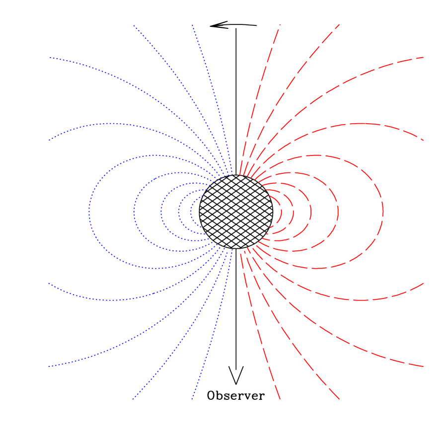
Figure 2: Illustration of isovelocity zones for a Keplerian disk. The hatched region at center is the star, assumed to rotate ccw, as indicated by the arrow at top. In this example an observer is located in the equatorial plane. Red curves on the right are for redshifted velocities (dashed), with the smallest loop having the greatest speed. Left are for blueshifts (dotted). Emission at line center arises from the vertical solid line.

2.2 Line Velocity Shifts

The Sobolev approximation is employed to describe the polarimetric line profiles. The Sobolev approach relies on identifying “isovelocity zones”, which are the locus of points that share the same Doppler shift for a distant observer. The Doppler shift in frequency of any point in the scattering volume is determined by

$$\Delta\nu_{\rm Z}=-\nu_{\rm ul}\,\frac{\mbox{$v_{\rm Z}$}}{c}=-\frac{\mbox{$v_{\rm Z}$}}{\lambda_{\rm ul}},$$ (1)

where $\nu_{\rm ul}$ is the frequency of the line transition, and $v_{\rm Z}$ is the line-of-sight velocity shift given by

$$\mbox{$v_{\rm Z}$}=-\vec{v}\cdot\mbox{$\hat{Z}$}.$$ (2)

A Keplerian disk follows a velocity profile of the form

$$\vec{v}=\mbox{$v_{\varphi}$}\,\mbox{$\hat{\varphi}$}=v_{0}\,\sqrt{\frac{R_{0}}{r}}\,\mbox{$\hat{\varphi}$},$$ (3)

where $R_{0}$ is the innermost radius of the disk with tangential speed $v_{0}$ at that location.

It is convenient to define dimensionless variables for distances and velocities. For the normalized cylindrical radius in the planar disk, $\varpi=r/R_{0}$ is used. The line-of-sight velocity shift then becomes

$$\mbox{$v_{\rm Z}$}=v_{0}\,\varpi^{-1/2}\,\sin i\,\sin\varphi.$$ (4)

A normalized velocity is also introduced with $\mbox{$w_{\rm z}$}=\mbox{$v_{\rm Z}$}/(v_{0}\sin i)$.

The solution for the isovelocity zones in terms of $\varpi(\mbox{$w_{\rm z}$},\varphi)$ is thus given by

$$\varpi=\frac{\sin^{2}\varphi}{\mbox{$w_{\rm z}^{2}$}}=\frac{\sin^{2}\varphi}{\sin^{2}\varphi_{0}}.$$ (5)

This describes a loop path that starts at $R_{0}$ at an azimuth $\varphi_{0}$ on the front side of the disk, where $\sin\varphi_{0}=\mbox{$w_{\rm z}$}$, and then ends again at $R_{0}$ and $\pi-\varphi_{0}$. The loop extends to a maximum distance at azimuth $\varphi=\pi/2$ with a value of $\varpi=1/\mbox{$w_{\rm z}^{2}$}$. The system is left-right mirror symmetric, with redshifted velocities on one side and blueshifted ones on the other. The convention here is that the disk rotates counterclockwise as seen from above (i.e., “prograde”). An example is displayed in Figure 2. With the arrow toward the observer as the reference for $\varphi$, redshifted velocities come from the interval $0<\varphi<\pi$, and blueshifted ones come from $\pi<\varphi<2\pi$.

2.3 Line Flux

For optically thin scattering, the observed flux of scattered light at a given velocity shift in the line is determined by a volume integral along the associated isovelocity loop. To describe the polarization, a Stokes vector prescription is adopted, with standard $I,Q,U,V$ notation. Referring back to Figure 1, an edge-on disk with $i=90^{\circ}$ would yield intensities with $Q>0$ and $U=0$. In this case “North” is chosen to be along the direction of $+\hat{Z}_{\ast}$, and $Q>0$ corresponds to oscillations of the electric vectors of the light being preferentially parallel to North.

For unresolved disks the corresponding observed fluxes are $\vec{\cal F}_{\nu}=(\mbox{${\cal F}_{I}$},\mbox{${\cal F}_{Q}$},\mbox{${\cal F}_{U}$},0)$, where it is assumed that the Stokes-V flux is zero for the problem at hand.

Generally following the notation of Paper II and using results from Ignace (2000a) for Keplerian disks, the disk is assumed to have a power-law surface number density given by

$$\Sigma(\varpi)=\Sigma_{0}\,\varpi^{-m},$$ (6)

for power-law exponent $m$ and inner value $\Sigma_{0}$ at $\varpi=1$. Note that in the case of the Be stars, values of $m$ range from 3–4 (e.g., Waters 1986; Lee, Osaki, & Saio 1991; Porter 1999; Jones, Sigut, & Porter 2008), and $m=3.5$ will be adopted in example cases. Implicit is that the lines of interest form from the dominant ion. Temperature and ionization variations or different disk densities could be included in the model, but the intent of this contribution is to highlight the line polarization and Hanle effect, and so a simple power-law density is adopted as a baseline for the analysis.

The Stokes fluxes for thin lines from this disk are given by

$$\vec{\cal F}_{\nu}(\mbox{$w_{\rm z}$})=\tau_{0}\,{\cal F}_{0}\,\int\,\mbox{$\vec{h}$}(\varpi,\varphi)\,\frac{\varpi^{2-m}}{w_{\varphi}(\varpi)}\,\frac{d\varpi}{|\cos\varphi|}.$$ (7)

The denominator in the integrand arises from the Sobolev approximation, with $w_{\varphi}=\varpi^{-1/2}$. The factor $|\cos\varphi|$ will more conveniently be written as $\sqrt{1-\mbox{$w_{\rm z}^{2}$}\varpi}$ in what follows. The vector $\vec{h}$ represents the “scattering factor” with $\mbox{$\vec{h}$}=(\mbox{$h_{I}$},\mbox{$h_{Q}$},\mbox{$h_{U}$},\mbox{$h_{V}$})$. It is this factor that incorporates the dipole scattering of resonance line polarization, the impact of magnetic fields via the Hanle effect, and the finite depolarization factor. Finally, the scaling factors outside the integral are from equations (24) and (25) of Paper II, with

$$\tau_{0}=\frac{\sigma_{l}\,\Sigma_{0}\,\lambda_{\rm ul}}{4\pi\,\mbox{$v_{\rm rot}$}\,\sin i},$$ (8)

where $\sigma_{l}$ is the frequency integrated line cross-section, and

$${\cal F}_{0}=\frac{L_{\nu,\ast}}{4\pi\,d^{2}},$$ (9)

where $L_{\nu,\ast}$ is the specific luminosity of the star and $d$ is the distance to the star from Earth.

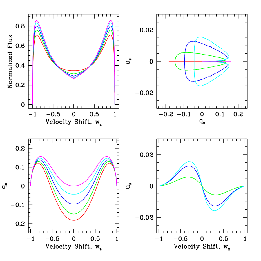
Figure 3: Line profiles for a disk with no magnetic field. Upper left: Area normalized Stokes-I line profiles for viewing inclinations of $i=0^{\circ}$ (red), $i=30^{\circ}$ (green), $i=45^{\circ}$ (dark blue), $i=60^{\circ}$ (light blue), and $i=90^{\circ}$ (magenta). Lower left: Stokes-Q profiles plotted as the ratio of the Q-flux to the scattered I-flux as fractional polarization (not percent). The yellow dashed line is a guide for zero polarization. Lower right: Like the Q-Profiles, Stokes-U profiles shown as fractional polarizations, which arise solely from the effect of stellar occultation. Upper right: A Q-U diagram across the profile.

2.4 Solution for Non-Magnetic Scattering Polarization

Before progressing to a consideration of the Hanle effect, there is value in formulating the solution for the line scattering polarization in the zero field case. This is because the Hanle effect primarily modifies the scattering polarization, meaning that a good understanding of the non-magnetic case is a necessary reference for understanding the Hanle effect. Many papers have dealt with line formation from Keplerian disks. This work draws in particular on the work of Huang (1961) and Rybicki & Hummer (1983) for planar disks, and also Ignace (2000a) for scattering polarization without the Hanle effect.

There are two main cases that are explored here: the simplistic case of illumination by a point source and then the more realistic case involving the effects of the finite size of the illuminating star. Analytic and semi-analytic solutions are described in the Appendices. The value of the point source approximation is that it gives context for how finite stellar size effects modify the line scattering polarization. The only portion of the point source approach that is reproduced here from Appendix A is the expression for isotropic scattering of starlight by a planar disk in the Sobolev approximation.

For isotropic scattering of light from a point star, one has $\mbox{$\vec{h}$}=(1,0,0,0)$. Only the Stokes-I flux survives in equation (7). It is convenient to introduce a change of variable for computing the integration of that equation, with $t=\varpi^{-1}$. Then the flux becomes

$$\mbox{${\cal F}_{I}$}=\tau_{0}\,{\cal F}_{0}\times 2\,\int_{t_{0}(w_{\rm z})}^{1}\,\frac{t^{m-1}}{\sqrt{t-t_{0}}}\,dt,$$ (10)

where $t_{0}=\mbox{$w_{\rm z}^{2}$}$. The appearance of the factor of 2 arises because the integration for the front half of the loop (from $\varphi_{0}$ to $\varphi=\pi/2$) is the same as for the back half.

Appendix A details analytic cases for the above case. The addition of polarization and finite source effects amount to inserting multiplicative “weighting” functions that modify the above integrand that describes the emission contribution as a function of location along a loop.

There are several finite source effects that can be included, such as finite star depolarization (Cassinelli et al. 1987), stellar occultation effects (e.g., Fox & Brown 1991), limb darkening effects (Brown, Carlaw, & Cassinelli 1989), and absorption of starlight by the disk (Ignace 2000a). Only two of these effects will be considered here: finite star depolarization and stellar occultation of the disk. Limb darkening could be included; however, limb darkening mainly “softens” the finite star depolarization factor, making it slightly less severe. Thus the inclusion of limb darkening does not seem to be a pressing issue for illustrating the Hanle effect in disks.

Absorption by the disk does affect the shape of the Stokes-I profile; however, in the current treatment it does not influence $\vec{h}$ which determines the line scattering polarization. Consequently, absorption affects the continuum level of direct starlight at the line, but not the scattered Stokes fluxes ${\cal F}_{I}$, ${\cal F}_{Q}$, or ${\cal F}_{U}$. On the other hand, a photospheric absorption line would alter the line shapes of the scattered flux profiles; however, results presented here will be in terms of ratios of scattered fluxes, $\mbox{$q_{\nu}^{\rm s}$}=\mbox{${\cal F}_{Q}$}/\mbox{${\cal F}_{I}$}$ and $\mbox{$u_{\nu}^{\rm s}$}=\mbox{${\cal F}_{U}$}/\mbox{${\cal F}_{I}$}$, for which the influence of a photospheric line will cancel.

These ratios $q_{\nu}^{\rm s}$ and $u_{\nu}^{\rm s}$ should be considered as polarimetric “efficiencies”. They are not generally what an observer would actually measure, because the denominator involves only the scattered light of the Stokes-I flux. Instead an observer would normally measure ${\cal F}_{Q}$, ${\cal F}_{U}$, and ${\cal F}_{\rm tot}={\cal F}_{0}+\mbox{${\cal F}_{I}$}$, the latter being the sum of the direct starlight (first term) and the scattered light (second term). In this case $q_{\rm tot}=\mbox{${\cal F}_{Q}$}/({\cal F}_{0}+\mbox{${\cal F}_{I}$})\approx\mbox{${\cal F}_{Q}$}/{\cal F}_{0}$, and likewise for the Stokes-U polarization, assuming that the scattered flux in the line is small compared to the direct flux by the star itself. As a result, $(q_{\rm tot},u_{\rm tot})=(\mbox{$q_{\nu}^{\rm s}$},\mbox{$u_{\nu}^{\rm s}$})\times(\mbox{${\cal F}_{I}$}/{\cal F}_{0})$. It is worth noting that the $q_{\nu}^{\rm s}$ and $u_{\nu}^{\rm s}$ “efficiency” profiles are independent of the line optical depth $\tau_{0}$ in the thin limit, since ${\cal F}_{I}$, ${\cal F}_{Q}$, and ${\cal F}_{U}$ scale linearly with $\tau_{0}$.

Equation B1 gives the scattering function components of $\vec{h}$ in the case of no magnetic field with the star treated as a point star of illumination. Modifications to those functions that allow for scattering by a finite sized and uniformly bright central star were determined in Paper III. For the case of zero magnetic field, the scattering function is shown explicitly with factors arising from the finite stellar size. These factors also appear in the scattering function with the Hanle effect in the same positions as without the Hanle effect. The vector components of $\vec{h}$ are:

$$\vec{h}=\left\{\begin{array}[]{lcl}h_{I}&=&\tilde{W}+\frac{3}{8}E_{1}\,\mbox{$\mu_{\ast}$}\,\left[\frac{1}{3}\,\left(1-3\cos^{2}i\right)\right.\\ &&\left.+\sin^{2}i\,\cos 2\varphi\right]\\ h_{Q}&=&\frac{3}{8}E_{1}\,\mbox{$\mu_{\ast}$}\,\left[\sin^{2}i\right.\\ &&\left.-\left(1+\cos^{2}i\right)\,\cos 2\varphi\right]\\ h_{U}&=&\frac{3}{8}E_{1}\,\mbox{$\mu_{\ast}$}\,\cos i\,\sin 2\varphi,\end{array}\right.$$ (11)

where

$$\tilde{W}=4\varpi^{2}\,W(\varpi),$$ (12)

with the dilution factor $W(\varpi)=0.5\,(1-\mbox{$\mu_{\ast}$})$, and

$$\mbox{$\mu_{\ast}$}=\sqrt{1-\varpi^{-2}}$$ (13)

is the finite depolarization factor when there is no limb darkening. The factors $\tilde{W}$ and $\mu_{\ast}$ represent corrections to the scattering function that account for the effects of finite star size in relation to the incident radiation field at a scattering point around the star.

Scattering by resonance lines can be approximated as part dipole and part isotropic. The parameter $E_{1}$ is a factor with values from 0 to 1 that represents the extent to which a resonance line scatters like a dipole radiator (see Chandrasekhar 1960). Only the dipole portion of the scattered light contributes to observable polarization. In the solar literature, it is more common to use the notation $W_{2}$ for the fraction of scattered light that is dipole-like (e.g., Stenflo 1978).

Accounting for stellar occultation breaks the back-front symmetry of the isovelocity loops. The front loop still has lower and upper limits of $t_{0}$ and 1, but the back half has limits of $t_{0}$ and $t_{\ast}\leq 1$. Here $t_{\ast}$ is associated with the minimum value of $\varpi=\varpi_{\ast}$ at the back-projected limb of the star corresponding to a maximum azimuth of $\varphi=\varphi_{\ast}$. An expression for $\varpi_{\ast}$ is given in Ignace (2000a), expressed here as

$$t_{\ast}=\sqrt{1-\sin^{2}i\cos^{2}\varphi_{\ast}}=\sqrt{\cos^{2}i-\mbox{$w_{\rm z}^{2}$}\sin^{2}i\,/t_{\ast}}.$$ (14)

This expression provides a cubic relation in $t_{\ast}$ as a function of fixed viewing inclination $i$ and velocity shift $w_{\rm z}$.

Numerical results for polarized profiles without the Hanle effect are shown in Figure 3. This Figure and the ones that will follow use $m=3.5$ and $E_{1}=0.5$. Figure 3 should be compared to Figure 9 for the point star case. For point star illumination, the maximum polarization occurs at the line wings and $\mbox{${\cal F}_{U}$}\equiv 0$ by symmetry. This changes dramatically when the effects of the finite stellar size are included.

In Figure 3, each panel has 5 curves color-coded for different viewing inclinations: $\sin^{2}i=0$ is red, $\sin^{2}i=0.25$ is green, $\sin^{2}i=0.5$ is deep blue, $\sin^{2}i=0.75$ is light blue, and $\sin^{2}i=1.0$ is magenta. The values correspond to viewing inclination angles of $i=0^{\circ},30^{\circ},45^{\circ},60^{\circ},$ and $90^{\circ}$, respectively. The upper left panel displays ${\cal F}_{I}$ profiles that are normalized to have unit area. In the lower right panel for the $q_{\nu}^{\rm s}$ polarization, the finite depolarization factor shifts peak polarization to lower velocity shifts as compared to the point star case, and $q_{\nu}^{\rm s}$ remains symmetric about line center. Stellar occultation leads to the survival of a small $u_{\nu}^{\rm s}$ polarization as shown in the lower right panel. The upper right panel is a $q_{\nu}^{\rm s}$-$u_{\nu}^{\rm s}$ plot across the respective line profiles. Note that the scales in $q_{\nu}^{\rm s}$ and $u_{\nu}^{\rm s}$ differ by about an order of magnitude. These small loops signify position angle rotations across the observed polarized line profiles, with polarization position angle $\psi_{P}$ given by $\tan 2\psi_{P}=\mbox{$u_{\nu}^{\rm s}$}/\mbox{$q_{\nu}^{\rm s}$}$.

We next turn our attention to the Hanle effect. The results of this section will prove valuable in following how the Hanle effect modifies the run of polarization across the line profile.

3 THE HANLE EFFECT IN KEPLERIAN DISKS

The Hanle effect applies to resonance line scattering and can be interpreted in semi-classical terms as a precession of an oscillating emitter that occurs over the radiative lifetime of the line emission. An angular quantity can be defined to represent the effective amount of precession, as given by

$$\tan\mbox{$\alpha_{2}$}=\frac{2\,g_{L}\,\omega_{L}}{A_{\rm ul}}=\frac{B}{\mbox{$B_{\rm Han}$}},$$ (15)

where $\omega_{L}$ is the angular Larmor frequency, $A_{\rm ul}$ is the Einstein radiative rate for the transition of interest, $g_{\rm L}$ is the Landé factor of the upper level, $B$ is the magnetic field strength in Gauss, and $B_{\rm Han}$ is the Hanle field sensitivity defined as

$$\mbox{$B_{\rm Han}$}=56.9\,\frac{A_{9}}{g_{\rm L}}~{}{\rm Gauss},$$ (16)

with $A_{9}$ the radiative rate normalized to $10^{9}$ Hz. The Hanle effect manifests itself in the scattering physics with the appearance of cosine and sine functions of the angle $\alpha_{2}$ (and a related quantity $\alpha_{1}=0.5\mbox{$\alpha_{2}$}$) within the scattering functions $\vec{h}$. Note that with no magnetic field, $B=0$ and $\mbox{$\alpha_{2}$}=0$. The limit of a high Larmor frequency yields $\mbox{$\alpha_{2}$}\approx\pi/2$. In this latter case, the Hanle effect is said to be “saturated”.

There are a few rules of thumb to help understand the Hanle effect in polarized lines. First, modifications to the polarized profile will depend on the orientation of the field in relation to both the direction of incoming radiation and outgoing radiation (i.e., the observer). Second there is no Hanle effect when the incoming radiation field is symmetric about the field direction. These first two “rules” indicate that there is no Hanle effect for radial magnetic fields (assuming a spherically symmetric star and no diffuse radiation) and that only non-radial components of the field contribute to modifying the polarization. However, the third point is that in spite of this, the angle $\alpha_{2}$ is sensitive to the total field strength: both radial and non-radial components, at the site of scattering. Fourth, and finally, the Hanle effect is sensitive only to the field topology in the saturated limit, not the field strength.

With these rules of thumb, consideration of the Hanle effect in three particular cases follow: a purely axial field, a purely toroidal field, and last a scenario involving fields as arising from the operation of MRI in disks.

3.1 Axial Magnetic Field

In this case an axial magnetic field is envisioned as threading the disk perpendicular to the equatorial plane, hence $\vec{B}=B_{Z_{\ast}}(\varpi)\,\hat{Z_{\ast}}$. As for the field distribution throughout the disk, the following is adopted as a conservative limiting case:

$$B_{Z_{\ast}}=B_{0}\,\varpi^{-1},$$ (17)

and so the Hanle angle $\alpha_{2}$ is determined by

$$\tan\mbox{$\alpha_{2}$}=\frac{B_{0}}{\mbox{$B_{\rm Han}$}}\,\varpi^{-1}\equiv b_{0}\,t.$$ (18)

where $b_{0}=B_{0}/\mbox{$B_{\rm Han}$}$ for $B_{0}$ a field strength at the inner disk radius. It is important to note that if $B_{0}\ll\mbox{$B_{\rm Han}$}$, then the Hanle effect is weak everywhere in the disk. If $B_{0}\gg\mbox{$B_{\rm Han}$}$, then the inner disk will be in the saturated limit; however, there will be a transition to a weak Hanle effect at some radius in disk, characteristically where $\varpi=B_{0}/\mbox{$B_{\rm Han}$}$. As a general rule, for a given magnetized disk, different lines will have different values of $B_{\rm Han}$, and thus will be sensitive to different aspects of the field at different locations in the disk.

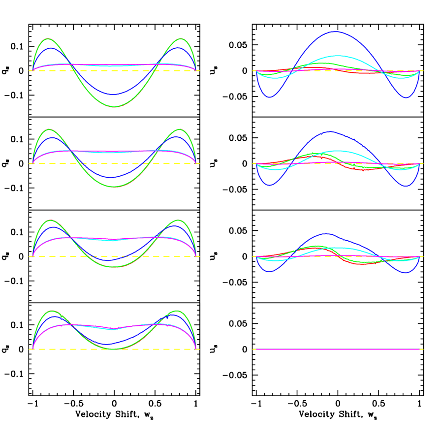
Figure 4: The Hanle effect for a disk threaded by a purely axial magnetic field. Left is for $q_{\nu}^{\rm s}$ and right is for $u_{\nu}^{\rm s}$. Profiles are shown for different viewing inclinations with $i=30^{\circ}$ at top, then $i=45^{\circ}$, $i=60^{\circ}$, and $i=90^{\circ}$ at bottom. The colors are for different field strengths with $b_{0}=0.01$ (red), 0.1 (green), 1.0 (dark blue), 10 (light blue), and 100 (magenta).

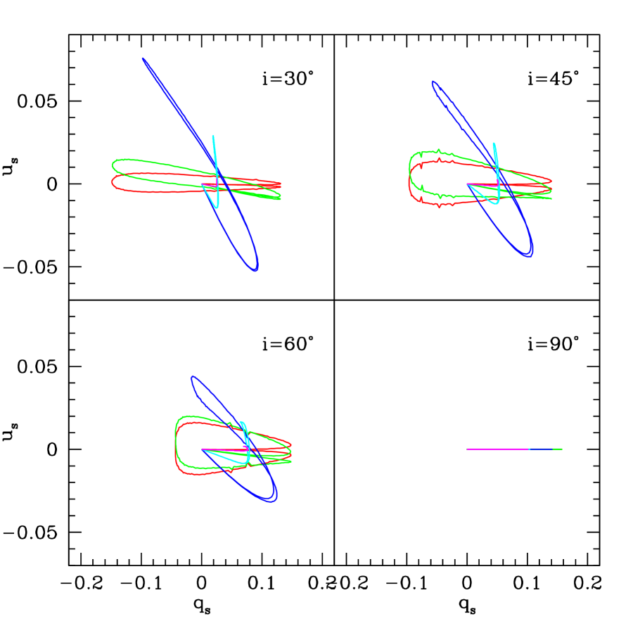
Figure 5: A Q-U diagram for the polarized profiles shown in Figure 4 with the same color scheme in relation to results for different values of $b_{0}$. The strongly “saturated” case of $b_{0}=100$ is present in magneta. This case has a modest range in $q_{\nu}^{\rm s}$ from 0 to about 0.1, but with $\mbox{$u_{\nu}^{\rm s}$}\approx 0$ everywhere, the profile is only a short horizontal line in the Q-U plane and difficult to see in this figure. For the edge-on case, $\mbox{$u_{\nu}^{\rm s}$}\equiv 0$ and all profiles degenerate to horizontal lines from 0 to a maximum value of $q_{\nu}^{\rm s}$ that depends on $b_{0}$.

Expressions for $\vec{h}$ in the point star limit are given in Appendix C. Revisions to those expressions for finite star depolarization and stellar occultation is the same as in equation (11). Results are shown in Figure 4. Profiles of $q_{\nu}^{\rm s}$ and $u_{\nu}^{\rm s}$ are displayed at left and right, respectively. Panels from top to bottom are now for different viewing inclinations of $\sin^{2}i=0.25,0.5,0.75,$ and 1.0. Different colors are for different values of $b_{0}$ with $b_{0}=0.01$ (red), 0.1 (green), 1.0 (dark blue), 10 (light blue), and 100 (violet).

The Stokes-Q profiles are symmetric about line center, whereas the U profiles evolve from weak and anti-symmetric, owing to stellar occultation, to strong and mostly symmetric, to a null profile at the strongly saturated limit. In the point star case, the saturated limit yields $\mbox{$u_{\nu}^{\rm s}$}=0$ and $\mbox{$q_{\nu}^{\rm s}$}=constant$ for all velocity shifts. With finite source effects, $q_{\nu}^{\rm s}$ is mostly flat throughout the central portion of the profile, but goes to zero in the wings. In the presence of limb darkening, the $q_{\nu}^{\rm s}$ profile would become more flattened toward the wings.

Figure 5 displays $q_{\nu}^{\rm s}$-$u_{\nu}^{\rm s}$ curves across the line profile. Note that the two axes have different scales: variations in $u_{\nu}^{\rm s}$ are smaller than for $q_{\nu}^{\rm s}$. The colored curves are the same cases as shown in Figure 4. Viewing inclinations are indicated. For the edge-on case of $i=90^{\circ}$, the curves are all degenerate with $\mbox{$u_{\nu}^{\rm s}$}=0$. The red loop is for a very weak field and is seen to be top-bottom symmetric in this space. As the field is increased, $q_{\nu}^{\rm s}$ and $u_{\nu}^{\rm s}$ profiles become individually more nearly symmetric. In the $q_{\nu}^{\rm s}$-$u_{\nu}^{\rm s}$ space, this results in curves with only small loops, for example the modest field case with the dark blue curve. As the disk enters the saturated limit, $u_{\nu}^{\rm s}$ drops to zero, $q_{\nu}^{\rm s}$ becomes somewhat flat-topped in appearance (again, except at the line wings), which degenerates mainly to a point in the $q_{\nu}^{\rm s}$-$u_{\nu}^{\rm s}$ space for most velocity shifts, with extension to zero polarization only for the line wings.

3.2 Toroidal Magnetic Field

A completely azimuthal field configuration has also been considered. As in the axial field case, the toroidal field strength is assumed to decrease inversely proportional to $\varpi$, and so equation (18) remains valid. This means that differences in the model polarized profiles between the axial and toroidal field configurations arise because the Hanle effect is sensitive to the vector field orientation.

As with previous considerations, some analytic results are derivable in the point star limit, and these are detailed in Appendix D for a disk with a toroidal field. With a toroidal field, the geometry associated with determining the Hanle effect is more complex than in axial field case. Geometrical relationships between the various angles defining the scattering problem with a toroidal field in a disk were given in the Appendix of Paper II and will not be repeated here. Results for the calculation of polarized profiles, including the effects of the star’s finite extent, are shown in Figure 6. This Figure is presented in the same manner as Figure 4 for the axial field case: $q_{\nu}^{\rm s}$ is at left and $u_{\nu}^{\rm s}$ at right; the panels are for different values of $\sin^{2}i$; the colors are for different field strengths characterized by $b_{0}$.

Note the marked differences in the line polarization between the toroidal case and that of an axial field. The Stokes-U profiles are always antisymmetric. Like the axial case, $q_{\nu}^{\rm s}$ profiles are symmetric, but the behavior is quite different. For example the edge-on disk case at lower left indicates that the profile polarization completely changes sign, from positive definite at every velocity shift when $B=0$ to everywhere negative in the saturated limit. This implies a $90^{\circ}$ rotation in position angle between these two limiting cases for the entire profile. For intermediate field strengths, there is a position angle rotation across the profile that occurs at different velocity shifts. In the axial field case, there is never a position angle rotation for an edge-on disk. For the $q_{\nu}^{\rm s}$-$u_{\nu}^{\rm s}$ shapes, differences in the polarizations are especially clear, with results for the toroidal field in Figure 7 to be compared against those for an axial field in Figure 5.

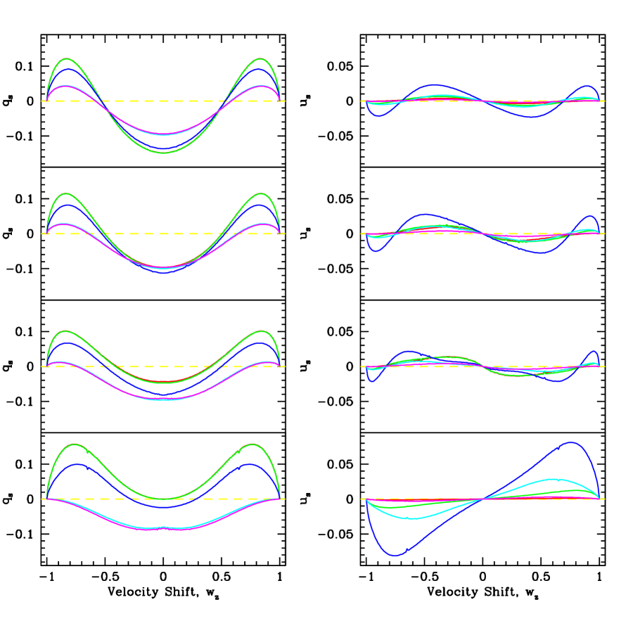
Figure 6: Similar to Figure 4 but now for a toroidal field instead of an axial one. From top to bottom, panels are for the same viewing inclinations, and the color scheme is for the same values of $b_{0}$. The $q_{\nu}^{\rm s}$ profiles are symmetric although differing in details from the axial field case. More striking is that the $u_{\nu}^{\rm s}$ profile is decidedly antisymmetric for the $B_{\varphi}$ case, whereas profiles tend toward being symmetric in the axial field case.

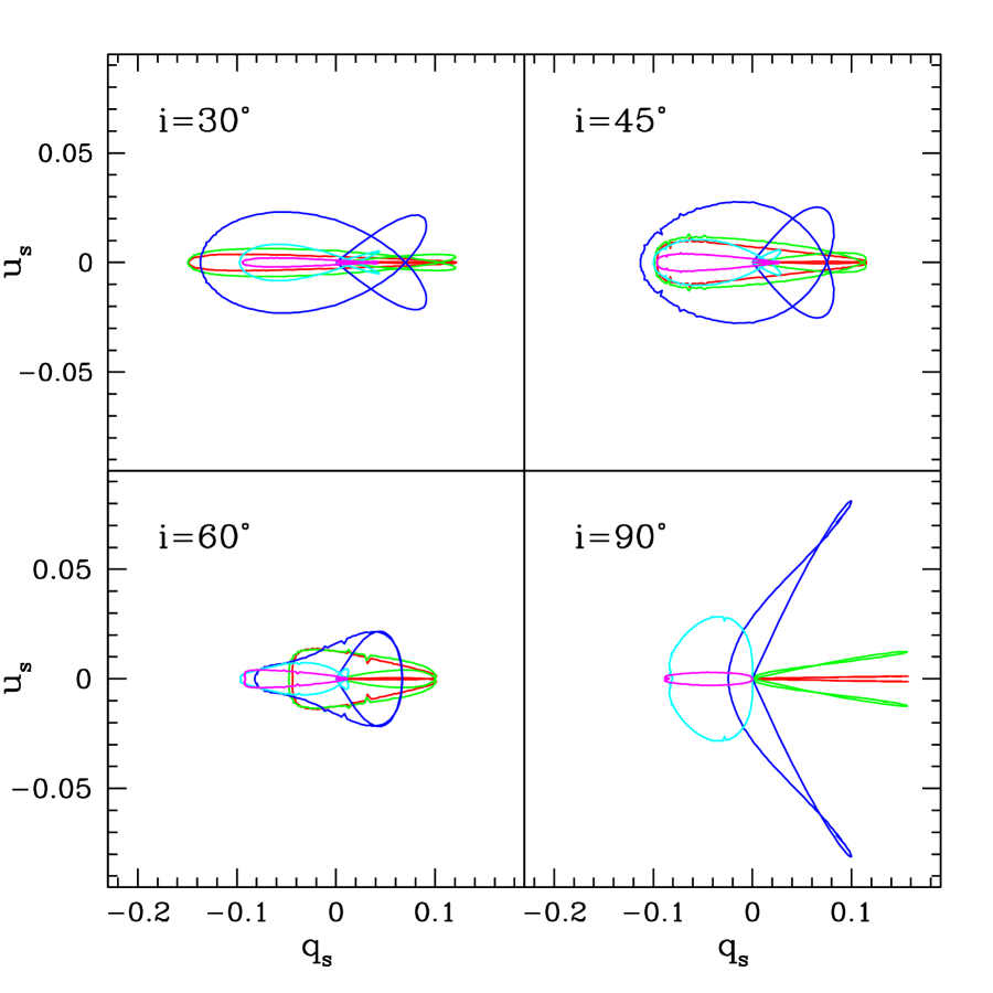
Figure 7: Similar to Figure 5 but now for a toroidal field instead of an axial one. The combination of antisymmetric $u_{\nu}^{\rm s}$ with symmetric $q_{\nu}^{\rm s}$ leads to Q-U loops that are top-bottom symmetric in this space. Note that the axis scale is different for $u_{\nu}^{\rm s}$ as compared to $q_{\nu}^{\rm s}$.

What is the source of these differences between the axial field and the toroidal one? The field orientation with respect to the viewer is clearly the key to the interpretation. For the axial case, the field at every point in the disk has some component of the magnetic vector directed toward the observer (if seen at $i<90^{\circ}$) or away from the observer (if seen at $i>90^{\circ}$). Thus, an axial field leads to a net projected magnetic flux of one sign or the other, which is true for every isovelocity loop. The toroidal field is manifestly different, since one side of the disk has components toward the observer and the other side has them away. For an axisymmetric toroidal field, the projected net magnetic flux is identically zero for the entire disk, but is oppositely signed in isovelocity loops for blueshifted velocities versus redshifted ones. In terms of the semi-classical precession description, flipping the field by $180^{\circ}$ amounts to a precession in the opposite direction. In the axial field case, the precession of the radiating oscillator is uniform – entirely clockwise (cw) or counterclockwise (ccw). Both cw and ccw precessions occur for a toroidal field configuration, with one precession occurring in half the line profile, and the opposite for the other half.

To illustrate this effect, Figure 8 shows line profile results for a toroidal field that now goes in the other direction as compared to Figure 6. The $q_{\nu}^{\rm s}$ profiles are nearly the same, but the $u_{\nu}^{\rm s}$ profiles are nearly mirror images of one another. slight differences are a result of the stellar occultation, which does not flip when the field orientation is reversed.

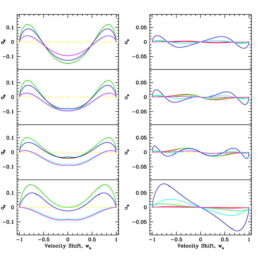
Figure 8: The same cases shown in Figure 6 except now for a toroidal field with the opposite sense of rotation. Note how the $u_{\nu}^{\rm s}$ profiles are essentially the reverse of those shown in Figure 6.

3.3 Magneto-Rotational Instability

A large literature has developed over the last twenty years in relation to the magnetorotational instability (MRI; Balbus & Hawley 1991, 1998). There is an interesting history about this effect (e.g., Balbus 2003). The instability can be illustrated through an analogy to two masses in a differentially rotating disk that are slightly offset from each other along a radius. These two masses are connected by a spring, to represent the effect of an axial magnetic field. The end result is that the two masses on different orbits seek to increase their displacement from one another. Coupling by the spring leads to a runaway situation ensues.

Key for the context of magnetic diagnostics is how this instability impacts the field topology and strength throughout the disk. The mass-spring analogy above has built into it the assumption of flux freezing. The separation of the masses along with the differential rotation would appear to evolve the axial field through the disk into a toroidal one. Different researchers have studied the operation of the MRI in accretion disks through both semi-analytic work and numerical simulations (e.g., Balbus & Hawley 1991, 1992; Hawley & Balbus 1991, 1992; Hawley, Gammie, & Balbus 1995; Hawley 2000; Fromang & Stone 2009; Lesur & Longaretti 2009; Maheswaran & Cassinelli 2009).

The goals of the MRI simulations are to understand better the physics of angular momentum transport through disks and disk structure. However, this paper seeks better insight into whether and how disk magnetism might be directly detected, with a focus on the Zeeman and Hanle effects for spectral lines. Ignace & Gayley (2008) reported on a simplistic calculation of the Zeeman effect and the Hanle effect for a Keplerian disk with a purely toroidal field. Here, application of the Hanle effect to Keplerian disks has been developed in a more complete way. But before discussing its application to the MRI scenario, it is worth commenting on the conclusions of Ignace & Gayley for the use of the Zeeman effect.

The MRI leads to a field topology that consists of a toroidal component and a randomized component. The toroidal components exists in mixed polarity, by which it is meant that some sectors run cw and others run ccw. For the weak longitudinal Zeeman effect, the Stokes-V flux scales with the net magnetic flux associated with a spatial resolution element (e.g., Mathys 2002). With bulk motions frequency (or wavelength or velocity) resolution ultimately maps to geometrical zones at the source (an example of this involving the Sobolev approximation was detailed by Gayley & Ignace 2010 for spherical winds). The key point is that if both the randomized field and the polarity of the toroidal component changes on small scales, then the flux of circularly polarized light arising from the Zeeman effect will be strongly suppressed owing to little net magnetic flux.

The issue of variations of the field on “small scales” must be evaluated with care. In the Sobolev approximation for purely Keplerian rotation, we have seen that the isovelocity zones are “loop” structures. These loops extend out to large radius for low velocity shifts, but they can be quite small at high velocity shifts. The highest velocity shifts degenerate to a pair of points for either limb of the star at the projected stellar equator! More importantly, every isovelocity zone intersects with the innermost radius of the disk. (If the disk extended down to the star, this would be the photospheric radius.) A steep power-law density ensures that the bulk of emission or scattered light comes from inner disk radii. As a result, the Zeeman effect would be most sensitive to a magnetic field at these locations, and thus “small scales” refers to turnovers in the field direction that are small compared to the inner radius of the disk. Consequently, the detection of the Zeeman effect from a disk with a given spectral resolution and density distribution constrains the characteristic spatial wavelengths at which the field turns over with radius from the star, azimuth around the star, and vertical height through the disk.

A detection of the Zeeman effect in a disk has previously been reported by Donati et al. (2005) in the case of FU Ori. This is thought to be an accretion disk with a disk wind, as evidenced by some lines showing P Cygni absorption. However, the circular polarization profile is argued as being associated with the innermost region of the rotating disk where the field is of kilogauss strengths. The detection implies a net magnetic flux per spectral resolution element, and thus sets limits on the turnover (or “tangledness”) length scale for the disk field, if indeed the MRI is operating in this case.

It is interesting to consider signals that could result with the Hanle effect. The Hanle effect can operate in regions where magnetic fields are “tangled” or randomized. This means that spatial averages of $\langle\vec{B}\rangle$ tend toward zero although $\langle B^{2}\rangle$ does not, such as is the case for the MRI mechanism. An extensive literature exists for the Hanle effect with random fields in applications to solar studies (e.g., Frisch et al. 2009, and references therein). Here I simply want to outline some of the limiting behavior in applications to disks.

Consider a Keplerian disk that contains everywhere a truly randomized magnetic field. If the field is weak at all locations, meaning that $B\ll\mbox{$B_{\rm Han}$}$, then of course a $q_{\nu}^{\rm s}$ line profile results as in the case of no Hanle effect. But if the field is strong, such that the denser regions of the disk are largely saturated, then the behavior is much different. With different field orientations, one expects that $u_{\nu}^{\rm s}$ will yield a null profile, by symmetry considerations. However, the $q_{\nu}^{\rm s}$ profile is different.

As a specific example, consider the resulting ${\cal F}_{Q}$ line from an edge-on disk. Without a field, the polarization at line center would be zero, owing to forward scattering of unpolarized starlight. With a randomized field, the polarization will still tend toward zero at line center. In the point star limit, some net polarization is expected to survive in the line wings. This polarization will be significantly reduced in comparison to the zero field case. If $E_{1}$ were unity, the polarization at the line wings would be 100%, since the scattering geometry is $90^{\circ}$. In analogy with considerations of scattering polarization off the solar limb, a reduction in polarization by a factor of 5 for isotropically distributed fields should be expected (see Stenflo 1982).

Now consider the introduction of a sustained toroidal field component. Of course toroidal fields were considered in the previous section. Now however, the toroidal field has polarity flips within the disk – $B_{\varphi}$ is alternately cw or ccw at essentially random points within the isovelocity zones. What this means is that there is a sign change in the direction of Larmor precession in the classical picture of a harmonic oscillator. The effect of this is to drive the $u_{\nu}^{\rm s}$ signal to zero faster than if the toroidal field had one sense of polarity. In the saturated limit, the $q_{\nu}^{\rm s}$ profile is unchanged, because the surviving polarized signal does not depend on polarity at all. This is quite different from the Zeeman effect that is sensitive to the net magnetic flux. For the Zeeman effect, the circular polarization will be suppressed when $B_{\varphi}$ switches polarity on small spatial scales.

4 CONCLUSIONS

Polarized line profile shapes from magnetized Keplerian disks have been calculated under a number of simplifying assumptions: the disk is geometrically thin; the scattering lines are optically thin; primarily simple fields were considered (axial or toroidal); and no account was taken of photospheric absorption lines. On the other hand, the model profiles do include finite source depolarization and the effects of stellar occultation. The presentation of results focused on the polarimetric “efficiencies” $q_{\nu}^{\rm s}$ and $u_{\nu}^{\rm s}$ with a description of how to identify the occurrence of the Hanle effect in scattering lines from disks. In addition, a discussion was presented for the Hanle effect from a magnetized disk in which the MRI mechanism is operating.

One of the main conclusions from this work is that axial and toroidal fields in disks are easily distinguishable through an analysis of $q_{\nu}^{\rm s}$-$u_{\nu}^{\rm s}$ figures for the run of Stokes polarizations across line profiles. Although a $u_{\nu}^{\rm s}$ profile does exist even without the Hanle effect, owing to stellar occultation, its amplitude is quite small. The strongest $u_{\nu}^{\rm s}$ profiles result when much of the inner disk, where most of the scattered light is produced, has values of $B/\mbox{$B_{\rm Han}$}$ of order a few. If the inner disk is mostly in the saturated limit of the Hanle effect, the $u_{\nu}^{\rm s}$ profile becomes a null profile for both axial and toroidal fields.

One should bear in mind that the polarized efficiencies are upper limits to the polarizations that would actually be measured, since the efficiencies are with reference to the scattered light only and do not take account of the direct starlight from the system. Since this starlight is expected to be largely unpolarized, its contribution acts to “dilute” the polarization substantially below the efficiency levels reported here. For example, if the line is relatively weak at 20% of the continuum level, then the expected measured polarizations would have fractional values at about 1/5 of the efficiency values, resulting in line polarizations of around 1%–2% for $q_{\nu}^{\rm s}$ and 0.5% or less for $u_{\nu}^{\rm s}$.

As percent polarizations, such values would appear to be easily measurable, but in practice there are several challenges. First, a spectral resolution yielding several points across the polarized profile is needed. Circumstellar disks have rotation speeds of order 500 km s^-1. A requisite velocity resolution of perhaps 50 km s^-1 would then be needed, implying a resolving power of $\lambda/\Delta\lambda\approx 6000$. Harrington & Kuhn (2009a) have demonstrated that such resolving powers can be achieved in spectropolarimetry; however, the next requirement is that of finding suitable scattering lines.

The very interesting effects seen in the sample of Harrington & Kuhn (2009a) exploits a relatively new effect of enhanced polarization that is coincident with regions of higher line absorption, a consequence of optical pumping effects. For the Hanle effect, or even for non-magnetic resonance scattering, lines that are predominantly scattering are needed. For hot star disks, such as the disks of Be stars, resonance scattering lines are generally to be found at UV wavelengths. This requires space-borne spectropolarimeters. Although the Wisconsin Ultraviolet Photo-Polarimeter Experiment (WUPPE) obtained exciting new results from UV polarimetry, its resolving power was only about 200 (Nordsieck et al. 1994). A new UV spectropolarimeter called the Far-Ultraviolet SpectroPolarimeter (FUSP) is a sounding rocket payload that will have a resolving power of about 1800 (Nordsieck 1998). Although possibly two low for circumstellar disks, it will be suitable for studying scattering line polarizations from high velocity stellar wind sources.

As a matter of practical analysis, how should spectropolarimetric data best be managed to measure a Hanle effect? Plotting the velocity shifted polarizations in the $q_{\nu}^{\rm s}$-$u_{\nu}^{\rm s}$ space appears to be most promising. The sequencing of the analysis for scattering lines from disk sources might proceed as follows:

• Subtract off the continuum polarization in the vicinity of the line of interest. This will counter the effects of both interstellar polarization and any other broadband source polarization, such as may arise from Thomson scattering in the disk.

• Plot the Q and U line fluxes, not fractional or percent polarizations that would be derived through normalization by the total I-flux. The reason for plotting polarized fluxes is that many common UV resonance lines are doublets (e.g., Nv, Siiv, and Civ UV resonance doublets). The shorter wavelength component (“blue”) has $E_{1}=0.5$, and the long wavelength component (“red”) has $E_{1}=0$ (e.g., Tab. 1 of Paper II). If the lines are thin, then the polarized flux from the red line will not be influenced by the blue one. However, if the lines are sufficiently closely spaced, then ${\cal F}_{I}$ will be a blend, and normalization by that blend would artificially skew the Q-U figure shape, making interpretation more difficult. If the doublet components are well separated, then relative polarizations could also be used in what follows.

• Determine whether the resultant figure for the line polarization shows any axis of symmetry. If so, then either (a) there is no Hanle effect, or (b) there is a Hanle effect with a dominant toroidal component. For an axis of symmetry, a rotation of the figure from observer Q-U axes to a source set of axes Q’-U’ could be accomplished with a Mueller rotation matrix. After rectifying the figure in this way, the relative amplitude of ${\cal F}_{U}$ should be compared to ${\cal F}_{Q}$. If $\mbox{${\cal F}_{U}$}\ll\mbox{${\cal F}_{Q}$}$, then there is likely little Hanle effect or the disk is in the saturated limit of the Hanle effect. If $\mbox{${\cal F}_{U}$}\sim\mbox{${\cal F}_{Q}$}$, then a Hanle effect is required with $b_{0}\approx$ few in the disk where the bulk of scattered light is produced. This means $B\approx\mbox{$B_{\rm Han}$}$.

• If there is no symmetry axis to the Q-U figure, then a Hanle effect involving an axial field is most likely the culprit. Recall that a radial field could be present, but this would give no Hanle effect by itself.

• For identifying a field distribution arising from MRI, things are more complicated. If the Hanle effect is in operation, then the Stokes-U flux is likely driven to zero, even if $b_{0}\sim 1$. A net ${\cal F}_{Q}$ profile should survive; however, it may not be symmetric. Using an oversimplification, each isovelocity zone can be considered to have a different effective $b_{0}$ value. This is already the case in the pure axial or toroidal field case that is axisymmetric, but the variation of the effective $b_{0}$ with velocity shift is monotonic (in a flux-weighted sense). With MRI, one expects non-monotonicity from fluctuations of the field strength. This amounts to the introduction of amplitude fluctuations across the polarized line.

There are complications to the above approach. For example, in the case of the Be star disks, there is substantial evidence for one-armed spiral density wave patterns that make the disk density non-axisymmetric (e.g., Okazaki 1997; Papaloizou & Savonije 2006). For thin Thomson scattering, there is little observational consequence of this effect which is mainly a redistribution of disk scatterers in a point antisymmetric pattern (e.g., Ignace 2000b). However, with resolved line profiles, the non-axisymmetric density distribution will produce asymmetry in the $q_{\nu}^{\rm s}$ profile and will be a new source of net $u_{\nu}^{\rm s}$ signal, also asymmetric. Certainly it will be important to model the ${\cal F}_{I}$ profile self-consistently along with the polarized profiles.

Note that there may be some concern about the choice adopted for the radial distribution of the field strength through the disk. The choice of $|\vec{B}|\propto\varpi^{-1}$ is perhaps the most shallow distribution that one could expect. A steeper gradient of the field strength will restrict the operation of the Hanle effect to a more restricted range of radii in the disk. If the interval in radius where $b_{0}\gtrsim 1$ becomes narrow in relation to where most of the scattered light is produced, then the Hanle effect will be irrelevant for the observed polarization.

What are the next steps in formulating better diagnostics of the density and magnetic field structure in disks? Most of work considered in this series of papers has focused on optically thin lines in an attempt to gain a better understanding of how the Hanle effect influences line polarizations that form in circumstellar media. In Paper IV the issue of optical depth effects for P Cygni lines from stellar winds were considered by treating regions of high optical as contributing no polarization at all. Although simplistic, insight was gained into how optical depth effects provide an additional spatial “filter” in terms of where bulk of line polarization will be produced. Naturally, rigorous radiative transfer and a more realistic disk model (i.e., not simply planar) is badly needed to extend the considerations of this paper. Even with thin line scattering, it would be useful to explore how non-axisymmetric disk models, such as the one-armed spiral density wave pattern for Be disks, will modify the line polarization. Moreover, winds driven off magnetized disks (e.g., Königl 1989; Proga, Stone, & Drew 1998; Proga, Stone, & Kallman 2000) have been ignored entirely in this work. These are all new calculations that will need to be considered in the future.

APPENDIX: SPECIAL CASES FOR THE LINE PROFILE SHAPES

In these Appendices, a number of instructional cases are considered for the polarized line profiles shapes from a Keplerian disk when the illuminating star is treated as a point source. This means that both stellar occultation and the finite star depolarization factor are ignored. A consequence of this approximation is that a non-zero $u_{\nu}^{\rm s}$ profile can only result from the Hanle effect. Before considering polarized line profiles, Stokes-I profile shapes are derived for the case of isotropic scattering. These solutions form the base emissivity function from which the polarized lines are constructed.

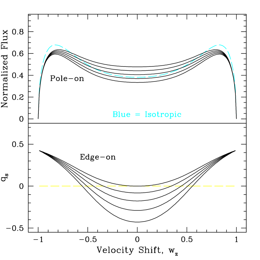
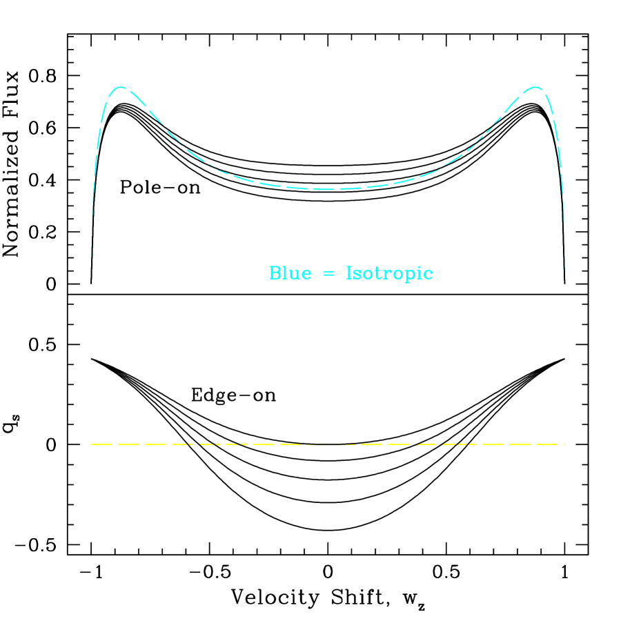
Figure 9: Analytic line profile shapes from isotropic scattering for the density exponent parameter $m=3$ at left and $m=4$ at right. The flux profiles are shown at top and $q_{\nu}^{\rm s}$ profiles at bottom. The different curves are for different viewing inclinations, with $\sin^{2}i=0.0,0.25,0.5,0.75$ and 1.0. In each case $E_{1}=0.5$. The flux profiles are normalized to the total line flux in the isotropic case. The normalized isotropic line is plotted in light blue in the upper panels.

Appendix A The Case of Isotropic Scattering

Isotropic scattering corresponds to $E_{1}=0$, and it means there is no polarization from resonance line scattering. Of course, that also means there is no Hanle effect, regardless of the field strength.

Even though there is no Hanle effect, the isotropic case is useful to explore as a reference for the production of the Stokes-I line shape. The integrand for the line emission as a function of velocity shift in the observed line represents the contributions by the disk density and the Sobolev effect for the profile shape. Allowing for $E_{1}\neq 0$ and the Hanle effect simply represents new weighting functions for non-isotropic scattering that multiply the integrand from the isotropic case.

The flux of line emission at normalized Doppler shift $w_{\rm z}$ is

$$\mbox{${\cal F}_{\nu}^{\rm iso}$}=\mbox{$\tau_{0}$}\,{\cal F}_{0}\times 2\int_{t_{0}}^{1}\,\frac{t^{\rm m-1}}{\sqrt{t-t_{0}}}\,dt,$$ (A1)

where the factor of 2 arises from the back-front symmetry of the integration along the isovelocity zone. As a reminder, $t=\varpi^{-1}$ and $t_{0}=\mbox{$w_{\rm z}^{2}$}$.

Again the preceding expression is only valid in the point star approximation. The power law exponent $m$ is from the surface density distribution that is assumed to be a power law of the form $\Sigma=\Sigma_{0}\,\varpi^{\rm-m}$. This formulation leads to symmetric double-peaked line profile shapes for $m>2$. Larger values of $m$ result in profiles that have more pronounced double-horns at greater velocity shifts from line center.

For integer values of $m$, the integral is analytic, and solutions for $m=3$ and $m=4$ are given here by way of example. For $m=3$ the result is

$$\mbox{${\cal F}_{\nu}^{\rm iso}$}(3)=\mbox{$\tau_{0}$}\,{\cal F}_{0}\times 2\int_{t_{0}}^{1}\,\frac{t^{2}}{\sqrt{t-t_{0}}}\,dt,=\mbox{$\tau_{0}$}\,{\cal F}_{0}\,\times\frac{4}{15}\,\left(3+4\mbox{$w_{\rm z}^{2}$}+8w_{\rm z}^{4}\right)\,\sqrt{1-\mbox{$w_{\rm z}^{2}$}},$$ (A2)

and for $m=4$,

$$\mbox{${\cal F}_{\nu}^{\rm iso}$}(4)=\mbox{$\tau_{0}$}\,{\cal F}_{0}\times 2\int_{t_{0}}^{1}\,\frac{t^{3}}{\sqrt{t-t_{0}}}\,dt,=\mbox{$\tau_{0}$}\,{\cal F}_{0}\,\times\frac{4}{7}\,\sqrt{1-\mbox{$w_{\rm z}^{2}$}}+\frac{6}{7}\,\mbox{$w_{\rm z}^{2}$}\,\mbox{${\cal F}_{\nu}^{\rm iso}$}(3).$$ (A3)

Note that increasing values of $m$ also result in profile shapes of lower amplitude. In fact it is possible to solve for the integrated light from a resonance scattering line in some special cases. Defining

$$F_{\rm tot}(m)=\int_{-1}^{+1}\,\mbox{${\cal F}_{\nu}^{\rm iso}$}\,d\mbox{$w_{\rm z}$},$$ (A4)

a few selected results are $F_{\rm tot}(1)=4\pi\cdot\mbox{$\tau_{0}$}{\cal F}_{0}$, $F_{\rm tot}(2)=5\pi/3\cdot\mbox{$\tau_{0}$}\,{\cal F}_{0}$, $F_{\rm tot}(3)=2\pi/3\cdot\mbox{$\tau_{0}$}\,{\cal F}_{0}$, and $F_{\rm tot}(4)=\pi/2\cdot\mbox{$\tau_{0}$}\,{\cal F}_{0}$.

It would appear that with $\mbox{$\tau_{0}$}=constant$, different values of $F_{\rm tot}$, and thus lines of different brightness levels, could result. This seems counterintuitive if lines characterized by different values of $m$ have the same optical depth. However, $\tau_{0}$ depends only on the density at the inner portion of the disk $\Sigma_{0}$, not the value of $m$. Thus when the line is optically thin, the appropriate optical depth to use is one that is angle averaged, similar in spirit to $\bar{\tau}$ in Brown & McLean (1977) for optically thin electron scattering. Hence use of a new optical depth parameter $T_{l}=\tau_{0}\times\tau_{0}{\cal F}_{0}/F_{\rm tot}(m)$ would ensure that lines of different $m$ values with isotropic scattering will have the same total line emission (i.e., “area under the curve”) even though they have different profile shapes.

Appendix B The Case of Resonance Scattering with $B=0$

For resonance line scattering with $E_{1}\neq 0$ but with $B=0$ everywhere, the vector scattering function $\vec{h}$ greatly simplifies. Following Paper II, we have that $\delta=\varphi$, $\alpha_{2}=0$, $C=\cos 2\varphi$, $D=\sin 2\varphi$, and $\mbox{$\psi_{\rm s}$}=0$. The components of the phase function become

$$\mbox{$\vec{h}$}=\left\{\begin{array}[]{lcl}h_{I}&=&1+\text@frac{3}{8}E_{1}\,\left[\text@frac{1}{3}\,\left(1-3\cos^{2}i\right)+\sin^{2}i\,\cos 2\varphi\right]\\ h_{Q}&=&\text@frac{3}{8}E_{1}\,\left[\sin^{2}i-\left(1+\cos^{2}i\right)\,\cos 2\varphi\right]\\ h_{U}&=&\text@frac{3}{8}E_{1}\,\cos i\,\sin 2\varphi.\end{array}\right.$$ (B1)

The Stokes flux of scattered light is

$$\vec{\cal F}^{\rm sc}=\mbox{$\tau_{0}$}\,{\cal F}_{0}\times 2\int_{t_{0}}^{1}\,\frac{t^{m-1}}{\sqrt{t-t_{0}}}\,\vec{h}\,dt.$$ (B2)

Note that care must be taken in dealing with terms that are odd and even in $\varphi$ between angles of 0 and $\pi$. For example, $h_{U}$ is odd around the loop, ensuring that ${\cal F}_{U}=0$. Accounting for the odd/even terms, and using the fact that $\sin^{2}\varphi=t_{0}/t=\mbox{$w_{\rm z}^{2}$}/t$, solutions for the scattered flux in Stokes-I and Stokes-Q are:

$$\mbox{${\cal F}_{I}$}^{\rm sc} = \left(1+\text@frac{1}{8}E_{1}-\text@frac{3}{8}E_{1}\cos 2i\right)\,\mbox{${\cal F}_{\nu}^{\rm iso}$}(m)-\text@frac{3}{4}E_{1}\,\sin^{2}i\,t_{0}\,\mbox{${\cal F}_{\nu}^{\rm iso}$}(m-1),$$ (B3)

$$\mbox{${\cal F}_{Q}$}^{\rm sc} = -\text@frac{3}{4}E_{1}\,\cos^{2}i\,\mbox{${\cal F}_{\nu}^{\rm iso}$}(m)+\text@frac{3}{4}E_{1}\,\left(1+\cos^{2}i\right)\,t_{0}\,\mbox{${\cal F}_{\nu}^{\rm iso}$}(m-1).$$ (B4)

Note at the extrema of the line wings, $\mbox{${\cal F}_{\nu}^{\rm iso}$}(m)=\mbox{${\cal F}_{\nu}^{\rm iso}$}(m^{\prime})$ and $t_{0}=1$, and $\mbox{$q_{\nu}^{\rm s}$}=3E_{1}/(4-E_{1})$ always.

The resultant polarization across the line is entirely in Stokes-Q when the observer’s reference axes are aligned with the symmetry axis of the star. With $E_{1}=0.5$, Figure 9 shows a plot of ${\cal F}_{I}^{\rm sc}$ for $m=3$ (left) and $m=4$ (right) at different viewing inclination angles of $i=0^{\circ},30^{\circ},45^{\circ},60^{\circ},$ and $90^{\circ}$ along the top panels. The profiles are normalized with respect to the total emission produced if the line had been isotropically scattering. At bottom is the relative fractional polarization $\mbox{$q_{\nu}^{\rm s}$}={\cal F}_{Q}^{\rm sc}/{\cal F}_{I}^{\rm sc}$ for $m=3$ and $m=4$ for the same viewing inclinations. Note that at the edges of the line, $\mbox{$q_{\nu}^{\rm s}$}=3/7$ for $E_{1}=0.5$, independent of the viewing inclination, as expected under the point star approximation.

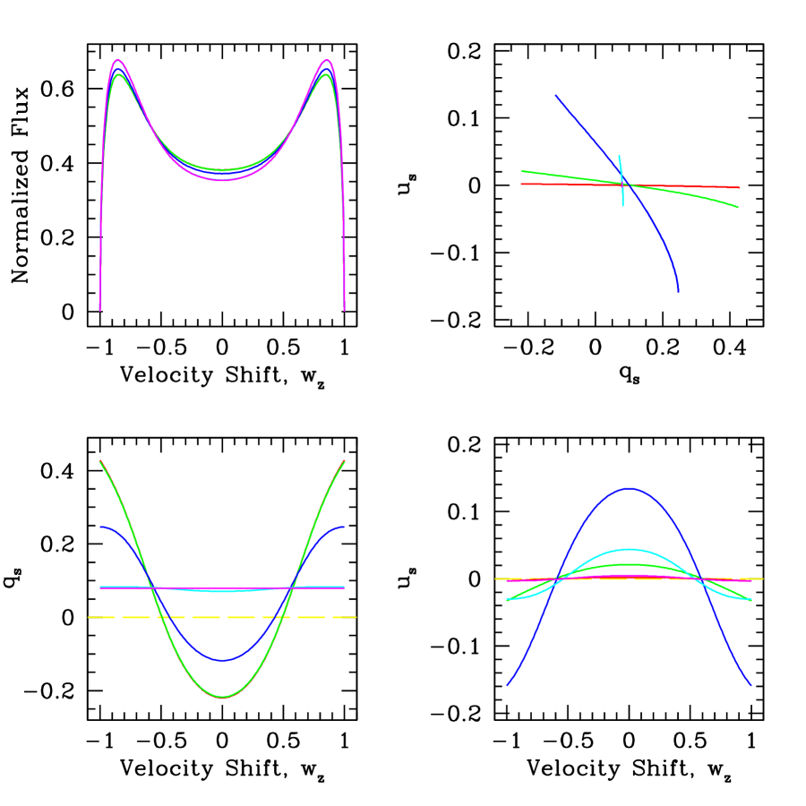
Figure 10: Similar to Fig. 5, here for the case of an axial field in the point star approximation.

The goal here is to illustrate the polarimetric “efficiency”. The actual measured fractional polarization would be much smaller owing to dilution by direct starlight. These efficiencty curves are relatively smooth functions of velocity shift. This smoothness is partly due to the fact that dipole scattering is a fairly slowly varying function of location around the disk and also because isovelocity loops sample a range of scattering angles.

Appendix C The Case of an Axial Field $B=B_{\rm Z_{\ast}}$

For an axial magnetic field with $\vec{B}=B_{\rm Z_{\ast}}(\varpi)\,\hat{Z}_{\ast}$, we have that $\mbox{$\psi_{\rm s}$}=0$ and $\mbox{$\theta_{\rm s}$}=i$. The scattering phase functions are quite similar to the zero field case, except that now the Hanle effect appears in factors in the functions $C$ and $D$. Using Paper II, the phase functions are given by

$$\vec{h}=\left\{\begin{array}[]{lcl}h_{I}&=&1+\text@frac{3}{8}E_{1}\,\left[\text@frac{1}{3}\,\left(1-3\cos^{2}i\right)+\sin^{2}i\,C(\varpi,\varphi)\right]\\ h_{Q}&=&\text@frac{3}{8}E_{1}\,\left[\sin^{2}i-\left(1+\cos^{2}i\right)\,C(\varpi,\varphi)\right]\\ h_{U}&=&\text@frac{3}{4}E_{1}\,\cos i\,D(\varpi,\varphi).\end{array}\right.$$ (C1)

where

$$C(\varpi,\varphi) = \phantom{-}\cos^{2}\alpha_{2}\cos 2\varphi-\text@frac{1}{2}\sin 2\alpha_{2}\sin 2\varphi$$ (C2)

$$D(\varpi,\varphi) = -\cos^{2}\alpha_{2}\sin 2\varphi-\text@frac{1}{2}\sin 2\alpha_{2}\cos 2\varphi,$$ (C3)

where

$$\cos^{2}\alpha_{2}=\frac{1}{1+b_{0}^{2}\,t^{2}},$$ (C4)

and

$$\cos\mbox{$\alpha_{2}$}\,\sin\mbox{$\alpha_{2}$}=\frac{b_{0}\,t}{1+b_{0}^{2}\,t^{2}}.$$ (C5)

Solutions for the vector Stokes flux is no longer analytic. With the Hanle effect, ${\cal F}_{U}\neq 0$ except for $B=0$ or in the saturated limit. In the latter case of $b_{0}\gg 1$ everywhere, an analytic solution can be obtained, which is given by

$${\cal F}_{I}^{\rm sc} = \left(1+\text@frac{1}{8}E_{1}-\text@frac{3}{8}E_{1}\cos 2i\right)\,\mbox{${\cal F}_{\nu}^{\rm iso}$}(m)$$ (C6)

$${\cal F}_{Q}^{\rm sc} = \text@frac{3}{4}E_{1}\,\sin^{2}i\,\mbox{${\cal F}_{\nu}^{\rm iso}$}(m).$$ (C7)

Note that in this limit, the relative polarization becomes

$$\mbox{$q_{\nu}^{\rm s}$}={\cal F}_{Q}^{\rm sc}/{\cal F}_{I}^{\rm sc}=\frac{3E_{1}\sin^{2}i}{8+E_{1}\,(1-3\cos^{2}i)},$$ (C8)

which is a constant across the profile and a function of viewing inclination only. This means that the polarized profile is flat-topped.

Figure 10 displays profiles for the axial field case with $E_{1}=0.5$ at a fixed value of $\sin^{2}i=0.4$ but with different field values at the inner disk radius of $\varpi=1$, of $\log b_{0}=-2,-1,0,+2,+4$ to achieve a large dynamic range in Hanle ratios throughout the disk. As $b_{0}$ increases, the location where $B=\mbox{$B_{\rm Han}$}$ moves outward to $\varpi=b_{0}$. The upper left panel in Figure 8 shows normalized profiles of ${\cal F}_{I}^{\rm sc}$; lower panels show the fractional polarizations $q_{\nu}^{\rm s}$ and $u_{\nu}^{\rm s}$; and upper right shows the $q_{\nu}^{\rm s}$-$u_{\nu}^{\rm s}$ shapes. The color sequencing is the same as in Figure 5. In large part the effect of an axial field is to rotate and foreshorten the Q-U segments relative to the zero field case.

Appendix D The Case of a Toroidal Field $B=B_{\varphi}$

For a toroidal magnetic field with $\vec{B}=B_{\varphi}\,\hat{\varphi}$, the spherical geometry for the scattering problem is moderately complex. It is not possible to write down simple complete expressions for the phase scattering functions. But as demonstrated in Paper II, there are still some special cases that are analytic. For example in the saturated limit, ${\cal F}_{U}^{\rm sc}=0$, and the $I$ and $Q$ fluxes become

$${\cal F}_{I}^{\rm sc} = \left(1+\text@frac{1}{8}E_{1}\right)\,\mbox{${\cal F}_{\nu}^{\rm iso}$}(m)-\text@frac{3}{8}E_{1}\sin^{2}i\,t_{0}\,\mbox{${\cal F}_{\nu}^{\rm iso}$}(m-1)$$ (D1)

$${\cal F}_{Q}^{\rm sc} = -\text@frac{3}{8}E_{1}\,\left[\mbox{${\cal F}_{\nu}^{\rm iso}$}(m)-(1+\cos^{2}i)\,t_{0}\,\mbox{${\cal F}_{\nu}^{\rm iso}$}(m-1)\right].$$ (D2)

For a disk viewed edge-on, solutions for the Stokes fluxes cannot be derived analytically; however, the scattering functions simplify to

$$\vec{h}=\left\{\begin{array}[]{lcl}h_{I}&=&1+\text@frac{3}{8}E_{1}\,\left(1-3\sin^{2}\varphi\right)+\text@frac{3}{8}E_{1}\,\cos^{2}\varphi\,\cos^{2}\alpha_{2},\\ h_{Q}&=&-\text@frac{3}{8}E_{1}\,\cos^{2}\varphi+\text@frac{3}{8}E_{1}\,(1+\sin^{2}\varphi)\,\cos^{2}\alpha_{2},\\ h_{U}&=&-\text@frac{3}{8}E_{1}\,\sin\varphi\,\sin 2\alpha_{2}.\end{array}\right.$$ (D3)

Examples of scattering and polarized profiles are shown in Figure 11 as well as Q-U plots across the polarized profiles. In the previous section, $\sin^{2}i=0.4$ was used for an axial field to give a significant signal in $u_{\nu}^{\rm s}$. For this toroidal field case, an edge-on disk with $\sin^{2}i=1.0$ was used. The style of this figure is the same as Figure 10. The a major distinctive in relation to a disk with an axial field is that a toroidal field leads to $u_{\nu}^{\rm s}$ profiles that are antisymmetric instead of symmetric.

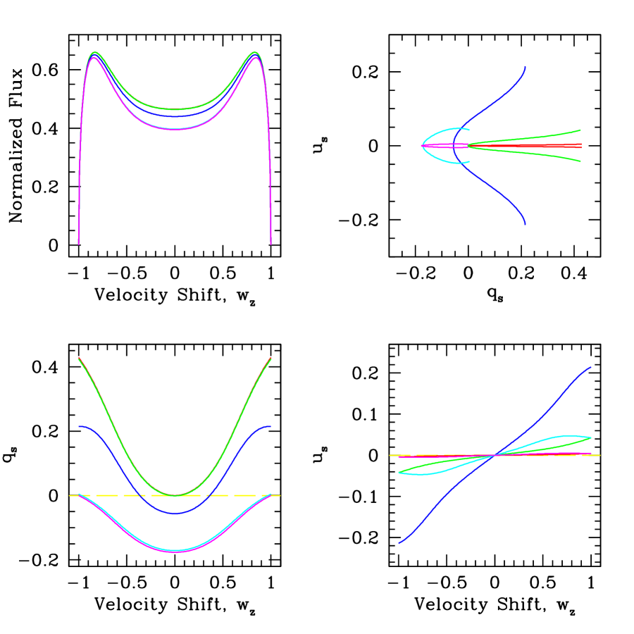
Figure 11: Similar to Fig. 10, here for the case of a toroidal field in the point star approximation.

References

- (1) Adamson, A., Aspin, C., Davis, C., Fujiyoshi, T. (eds) 2005, Astronomical Polarimetry: Current Status and Future Directions, ASP Conf. Ser. #343
- (2) Balbus, S. A. 2003, ARAA, 41, 555
- (3) Balbus, S. A., Hawley, J. F. 1991, ApJ, 376, 214
- (4) Balbus, S. A., Hawley, J. F. 1992, ApJ, 400, 610
- (5) Balbus, S. A., Hawley, J. F. 1998, Revs. of Mod. Physics, 70, 1
- (6) Bastian, P. (ed) 2010, Astronomical Polarimetry 2008-Science from Small to Large Telescopes, ASP Conf. Ser., to appear
- (7) Brown, J. C., McLean, I. S. 1977, A&A, 57, 141
- (8) Brown, J. C., Carlaw, V. A., Cassinelli, J. P. 1989, ApJ, 344, 341
- (9) Cassinelli, J. P., Nordsieck, K. H., Murison, M. A., 1987, ApJ, 317, 290
- (10) Chandrasekhar, S. 1960, Radiative Transfer (New York: Dover)
- (11) Cranmer, S. R. 2009, ApJ, 701, 396
- (12) Donati, J.-F., Babel, J., Harries, T. J., Howarth, I. D., Petit, P., Semel, M. 2002, MNRAS, 333, 55
- (13) Donati, J.-F., Howarth, I. D., Jardine, M. M., Petit, P., Catala, C., Landstreet, J. D., et al. 2006a, MNRAS, 370, 629
- (14) Donati, J.-F., Howarth, I. D., Bouret, J.-C., Petit, P., Catala, C., Landstreet, J. 2006b, MNRAS, 365, L6
- (15) Donati, J.-F., Landstreet, J. D., 2009, ARAA, 47, 333
- (16) Donati, J. F., Paletou, F., Bouvier, J., Ferreira, J., 2005, Nature, 438, 466
- (17) Donati, J.-F., Semel, M., Carter, B. D., Rees, D. E., Collier Cameron, A., 1997, MNRAS, 291, 658
- (18) Fox, G. K., Brown, J. C. 1991, ApJ, 375, 300
- (19) Frisch, H., Anusha, L. S., Sampoorna, M., Nagendra, K. N. 2009, A&A, 501, 335
- (20) Fromang, S., Stone, J. M. 2009, A&A, 507, 19
- (21) Gayley, K. G., Ignace, R. 2010, ApJ, 708, 615
- (22) Grunhut, J. H., Wade, G. A., Marcolino, W. L. F., Petit, V., Henrichs, H. F., et al. 2009, MNRAS, 400, L94
- (23) Hanle, W. 1924, Z. Phys., 30, 93
- (24) Harrington, D. M., Kuhn, J. R., 2009a, ApJS, 180, 138
- (25) Harrington, D. M., Kuhn, J. R., 2009b, ApJ, 695, 238
- (26) Harries, T. J. 2000, MNRAS, 315, 722
- (27) Hawley, J. F., 2000, ApJ, 528, 462
- (28) Hawley, J. F., Balbus, S. A. 1991, ApJ, 376, 223
- (29) Hawley, J. F., Balbus, S. A. 1992, ApJ, 400, 595
- (30) Hawley, J. F., Gammie, C. F., Balbus, S. A. 1995, ApJ, 440, 742
- (31) Hole, K. T., Kasen, D., Nordsieck, K. H. 2010, ApJ, 720, 1500
- (32) Huang, S.-S. 1961, ApJ, 133, 130
- (33) Ignace, R., 2000a, A&A, 363, 1106
- (34) Ignace, R., 2000b, in The Be Phenomenon in Early-Type Stars, M. A. Smith, H. F. Henrichs (eds), IAU Colloq. #175, ASP, Conf. Ser. 214, 452
- (35) Ignace, R., 2001, ApJ, 547, 393 (Paper III)
- (36) Ignace, R., Cassinelli, J. P., & Nordsieck, K. H., 1999, ApJ, 520, 335 (Paper II)
- (37) Ignace, R., Gayley, K. G., 2008, in Clumping in Hot-Star Winds, (eds) W.-R. Hamann, A. Feldmeier, L. M. Oskinova,
- (38) Ignace, R., Nordsieck, K. H., & Cassinelli, J. P., 1997, ApJ, 486, 550 (Paper I)
- (39) Ignace, R., Nordsieck, K. H., & Cassinelli, J. P., 2004, ApJ, 609, 1018 (Paper IV)
- (40) Jones, C. E., Sigut, T. A. A., Porter, J. M. 2008, MNRAS, 386, 1922
- (41) Königl, A. 1989, ApJ, 342, 208
- (42) Kuhn, J. R., Berdyungina, S. V., Fluri, D. M., Harrington, D. M., Stenflo, J. O. 2007, ApJ, 668, L63
- (43) Landi Degl’Innocenti, E., Landolfi, M. 2004, Polarization in Spectral Lines, Astrophysics and Space Library, v. 307 (Kluwer: Dordrecht)
- (44) Lee, U., Osaki, Y., Saio, H. 1991, MNRAS, 250, 432
- (45) Lesur, G., Longaretti, P.-Y. 2009, A&A, 504, 309,101
- (46) Maheswaran, M., Cassinelli, J. P. 2009, MNRAS, 394, 415
- (47) Mathys, G. 2002, in Astrophysical Spectropolarimetry, (eds.) J. Trujilo-Bueno, F. Moreno Insertis, F. Sanchez, 101
- (48) Neiner, C., Geers, V. C., Henrichs, H. F., Floquet, M., Fremat, Y., Hubert, A.-M., et al. 2003, A&A, 406, 1019
- (49) Nordsieck, K. H., Marcum, P., Jaehnig, K. P., & Michalski, D. E. 1994, Proc SPIE, 2010, 28
- (50) Nordsieck, K. H. 1998, in Ultraviolet-Optical Space Astronomy Beyond HST (ASP Conf Series), in prep.
- (51) Okazaki, A. T. 1997, A&A, 318, 548
- (52) Papaloizou, J. C. B., Savonije, G. J. 2006, A&A, 456, 1097
- (53) Porter, J. M. 1999, A&A, 348, 512
- (54) Proga, D., Stone, J. M., Drew, J. E. 1998, MNRAS, 295, 595
- (55) Proga, D., Stone, J. M., Kallman, T. R. 2000, ApJ, 543, 686
- (56) Rybicki, G. B., Hummer, D. G. 1983, ApJ, 274, 380
- (57) Sobolev, V. 1960, Moving Envelopes of Stars (Mass.: Harvard Univ.)
- (58) Stenflo, J. O. 1978, A&A, 66, 241
- (59) Stenflo, J. O. 1982, Solar Phys., 32, 41
- (60) Stenflo, J. O. 1994, Solar Magnetic Fields (Dordrecht: Kluwer)
- (61) Trujillo Bueno, J., Landi Degl’Innocenti, E., 1997, ApJ, 482, L183
- (62) Vink, J. S., Harries, T. J., Drew, J. E. 2005, A&A, 430, 213
- (63) Wade, G. A., Alecian, E., Bohlender, D. A., Bouret, J.-C., Grunhut, J. H., Henrichs, H., et al. 2009, in Cosmic Magnetic Fields: From Planets, to Stars and Galaxies, IAU Symp. #259, 333
- (64) Waters, L. B. F. M. 1986, A&A, 162, 121
- (65) Wang, L., Wheeler, J. C. 2008, ARAA, 46, 433
- (66) Wood, K., Brown, J. C., & Fox, G. K. 1993, A&A, 271, 492
- (67)