Discrete Constant Mean

Curvature Surfaces

via Conserved Quantities

Wayne Rossman

Forward

These notes are about discrete constant mean curvature surfaces defined by an approach related to integrable systems techniques. We introduce the notion of discrete constant mean curvature surfaces by first introducing properties of smooth constant mean curvature surfaces. We describe the mathematical structure of the smooth surfaces using conserved quantities, which can be converted into a discrete theory in a natural way.

About referencing: We do not attempt to give a complete reference list, and omit what is already referenced in [59]. We list only articles referenced in the body of the text, or that were written after [59] was published, or were otherwise not included in the reference list in [59], or that were referenced in [59] but need to be updated.

About using quaternions: In following with the historical development of the field, we use a model that involves quaternions. However, the use of a more standard model has some advantages, as it can be applied in more general dimensions and settings (see Chapter 10 here, for example), and sometimes gives less cluttered computations. It would be a good exercise to convert this text into one involving a more standard quaternion-free model, but we do not do that here (see [27]), and instead only make occasional comments about this.

Acknowledgements: Primary thanks must go to Udo Hertrich-Jeromin, who carefully and patiently taught the author more than half of the material in this text. The author also owes thanks to many others for numerous mathematical tips: Fran Burstall, Tim Hoffmann, Boris Springborn, Ulrich Pinkall, Masaaki Umehara, Kotaro Yamada, Takeshi Sasaki, Masaaki Yoshida, Masatoshi Kokubu, Shoichi Fujimori, Shimpei Kobayashi, Yusuke Kinoshita and Tetsuhiro Tachiyama amongst them.

Also, the author would like to express his gratitude to the Kyushu University GCOE program for giving him the opportunity to present the material in this text in a short course at Kyushu University in February of 2010.

It goes without saying that I, the author, am solely responsible for choices of approaches and for any possible errors.

1. Motivations for studying CMC surfaces

These notes are about surfaces of constant mean curvature, or, more briefly, ”CMC” surfaces. In particular, we will focus on discrete versions of CMC surfaces. However, it is useful to first take a close look at the smooth case, so let us start there.

Smooth CMC surfaces can be thought of as mathematical models for soap films, or we might say that they are ”mathematically perfect” soap films. Saying that CMC surfaces are models for soap films is certainly not a rigorous mathematical definition, but it is a good starting point for appreciating why CMC surfaces are interesting objects. In fact, it would be impossible to explain why mathematicians have put so much effort into understanding CMC surfaces without discussing soap films, or interfaces between fluids, or some other similar idea. Even though modern-day research on CMC surfaces might not always relate immediately to soap films, the notion of soap films is invariably lurking in the background. So let this be our first informal definition:

CMC surfaces are soap films.

In fact, CMC surfaces are defined to be those surfaces whose mean curvature is constant, as their name suggests. But we save a rigorous definition of mean curvature for later. This rigorous definition is locally equivalent to the above informal definition, and we also explain this later.

1.1. Soap films

A soap film forms a surface that minimizes area with respect to some given constraints, and it is the constraints that determine which soap film will be formed. Let us give some examples, all of which can be physically constructed if one has the necessary ingredients:

1. If one puts a circular wire ring into a fluid soap solution and then extracts it, one obtains a soap film that is a flat planar disk with this ring as its boundary. Here the only constraint on this soap film is its boundary, which is fixed to be a round circle, and this boundary constraint then determines the resulting soap film (the flat planar disk).

2. Blowing sufficiently hard on the above flat round disk in item (1) above would cause this soap film to break free of the circular ring and become a free floating round sphere. (This activity is a common pastime for young children.) This sphere contains a pocket of air of a certain volume, and since this air cannot escape to the other side of the soap film, this volume is fixed. Here the only constraint on this soap film is the fixed volume it contains. With respect to this volume constraint, the soap film minimizes its area, and the round sphere is the unique shape that accomplishes this.

3. Taking two circular wire rings of the same radius, we can produced two flat soap films in the shapes of round disks, as in item (1). Putting these two disks together so that they coincide and then pulling them slightly apart in the direction perpendicular to the planes they lie in results in a soap film that has three smooth pieces meeting along a singular round circle. Two of the smooth pieces are surfaces of revolution and are reflections of each other across the plane that is midway between the two parallel planes containing the two circular wire rings. The third smooth piece is a flat planar disk contained in that plane of reflection. If one pushes a dry pointed object (such as a pencil) into the third smooth piece, then the soap film will instantly pop into a single smooth anvil-shaped surface of revolution. This last soap film is called a catenoid. It is determined by its boundary constraint, which is two fixed circular wire rings.

4. Taking the catenoidal soap film in the previous example, we can place two flat plastic disks so that they fill the planar regions inside the two boundary circular wires. We have then trapped air inside the catenoid. Making a small hole in one of the plastic disks and pumping more air into this interior region (through that hole), the sides of the anvil-shaped catenoid will expand to accommodate the increase of volume inside. If just the right amount of air is pumped in (and if the two boundary circular wires are not too far from each other), the soap film will become exactly a portion of a round cylinder. Thus the round cylinder can be made using a soap film. In this case there are two constraints. One constraint is the fixed boundary (two circular wire rings in parallel planes), and the other is the fixed volume (inside the cylinder). Other surfaces of revolution can be made from soap films in this way by pumping air into the interior region, and these surfaces turn out to be portions of Delaunay surfaces, which we have described in detail in [59].

These examples show that the flat plane, the round sphere, the catenoid and the round cylinder are all CMC surfaces.

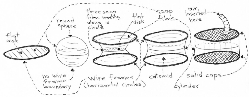
Figure 1. The soap films described in items (1), (2), (3) and (4) at the beginning of Chapter 1.

Amongst the four examples above, only the second and fourth ones have any volume constraints. The volume constraints in these two cases are that the volume to one side of the surface is constrained to be a fixed quantity. In the case that there are only boundary constraints and no volume constraints (as in the first and third examples), the resulting soap film is a special case of a CMC surface that is called a minimal surface. Thus the flat plane and catenoid are minimal surfaces. In the case that there are volume constraints (as in the second and fourth examples), the resulting soap film is a non-minimal CMC surface. Thus the round sphere and round cylinder are non-minimal CMC surfaces.

1.2. Interfaces

More generally, CMC surfaces are models for the interface between two distinct uniform fluids. For example, when one pours some lighter-than-water oil into a cup of water, the oil will rise to the top and the interface between the oil and the water will become a flat horizontal plane, a minimal surface. If one has two types of oils of equal density that do not like to interact with each other, and one puts a small amount of one type into a glass container filled with the other type, then the first type will take the shape of a round ball floating in the other type. Since this ball is round, the interface between the two oils will be the CMC surface that is a round sphere. (In the presence of gravity, the interface between two distinct uniform non-interacting fluids can be a more general type of surface called a capillary surface, not always a CMC surface. Robert Finn has done much work on capillary surfaces; see [54], [55], [56], [57] for nice introductions to the subject.)

1.3. Variational property

That soap films minimize area with respect to some given constraints is called a variational property, because this minimization property can be rephrased in the following way: If one continuously varies (deforms) the soap film so that its given constraints are preserved, then the area of the soap film will increase. Thus soap films minimize area under continuous variations that preserve the constraints. Once we give a formal definition of CMC surfaces, we will see that CMC surfaces are a larger class of surfaces than soap films, in part because CMC surfaces include nonphysical objects called ”unstable” soap films, and so the above statement is not strictly true for CMC surfaces. However, this is a technical point that we can ignore for the moment, and simply note that the above variational property turns out to still be true for small pieces of CMC surfaces: If one continuously varies a sufficiently small portion of a CMC surface so that its given constraints are still preserved, then the area of the varied surfaces will be larger than that of the original CMC surface. Thus we can give a second definition for CMC surfaces that is still informal, but is intuitively useful:

CMC surfaces are surfaces that locally minimize area with respect to boundary and volume constraints.

We will describe the meaning of an ”unstable” CMC surface in more detail in Section 2, and we will see some examples there.

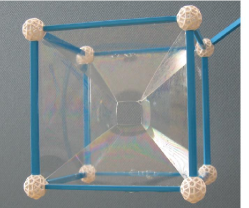
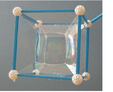
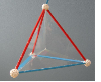
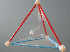
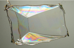
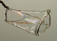
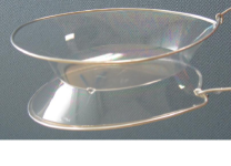
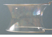
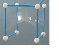
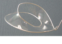
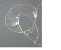
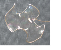
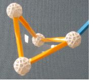
Figure 2. Examples of soap films. Whenever surfaces come together along a singular edge, they meet in threes and come together at $120$ degree angles, and whenever those singular edges meet at a singular vertex, they meet in fours and come together at the tetrahedral angle (approximately $109$ degrees).

1.4. Connections with other fields

Because CMC surfaces model soap films and interfaces between fluids, they have connections to physics, chemistry and polymer science. In fact, sometimes new examples of these surfaces are discovered by people in these other fields rather than by differential geometers. (One example of this are the minimal surfaces found by Fischer and Koch [58], see Figure 3.4.10 in [59].) CMC surfaces have connections with biology as well, and an example of this is that some forms of coral take shapes resembling the triply periodic Schwarz P minimal surface in Figure 3. CMC surfaces are even sometimes connected to architecture, as can be seen by looking at the Olympic Stadium in Munich, which has sheets resembling minimal surfaces. Thus is it clear that CMC surfaces have connections to fields outside of mathematics, and this is certainly one of the reasons why we study them.

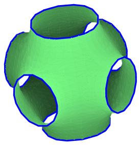
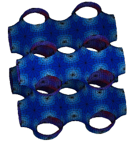
Figure 3. The minimal triply-periodic Schwarz P surface.

1.5. Connections within mathematics

Other reasons for studying CMC surfaces are that they have a rich mathematical structure and have interesting relations to other fields within mathematics. Although minimal and CMC surfaces are topics of geometry, they are also fundamental examples in the calculus of variations, as is clear from the variational property that we described above. Thus minimal and CMC surfaces are closely connected to the calculus of variations (although we will explore this connection only briefly in Section 2).

Minimal surfaces are also strongly related to the field of complex analysis via a theorem called the Weierstrass representation (this representation was given in [59]). This representation provides a way to describe all minimal surfaces using pairs of complex-analytic functions defined on Riemann surfaces. As a result, the theory of minimal surfaces has a rich mathematical structure and has many easily accessible examples. A number of the simpler examples were described in [59].

Also, by making use of an additional parameter (called the spectral parameter), one can describe non-minimal CMC surfaces as well in terms of complex-analytic functions defined on Riemann surfaces (see [59]). Hence again we have a connection to the field of complex analysis. Furthermore, away from isolated special points (umbilics), non-minimal CMC surface theory is equivalent to the sinh-Gordon equation. This equation appears prominently in the theory of integrable systems, so CMC surfaces are also clearly connected to that field. In fact, the essential idea behind the DPW method, which we focused on in [59], comes from the theory of integrable systems. The DPW method is a method for constructing CMC surfaces using loop group techniques coming from the theory of integrable systems. Finally, we note that both the minimal and non-minimal CMC surface equations are well-known partial differential equations, so the connection of these surfaces to the field of partial differential equations is evident.

Applying the techniques of these other fields of mathematics to CMC surfaces gives these surfaces a rich mathematical structure and gives us the means to describe many examples of CMC surfaces, as we saw in [59].

1.6. Non-Euclidean ambient spaces

When we move to studying CMC surfaces in spaces other than Euclidean $3$-space $\mathbb{R}^{3}$, the connections to chemistry, polymer science, biology and architecture certainly largely disappear, but connections to physics still remain – and the strong connections to other fields within mathematics remain completely intact, as we can find other ambient spaces for which the rich mathematical structure of CMC surfaces and their connections to other mathematical fields carry over. In some ways the mathematical structure carries over in an analogous way from the case of $\mathbb{R}^{3}$, but in some ways the structure changes in interesting ways. The behavior of the direction perpendicular to the surface (the Gauss map) can behave quite differently in other 3-dimensional ambient spaces, and the global properties of the CMC surfaces can be markedly different. In this text, we will study CMC surfaces (and some other types of surfaces as well) in the spaces $\mathbb{S}^{3}$, $\mathbb{H}^{3}$ and $\mathbb{R}^{2,1}$ that we will define later in this text.

1.7. Discrete CMC surfaces

Recently, finding discrete analogs of smooth objects has become an important theme in mathematics, appearing in a variety of places in analysis and geometry. So it is natural to consider discrete analogs of smooth minimal and CMC surfaces. But there is no single definitive approach; the definition one chooses depends on which properties of smooth minimal and CMC surfaces one wishes to emulate in the discrete case.

One can define a discrete minimal surface in Euclidean $3$-space ${\mathbb{R}^{3}}$ to be a piecewise linear triangulated surface that is critical for area with respect to any compactly-supported boundary-fixing continuous piecewise-linear variation (of its vertices) that preserves its simplicial structure, see [134]. Then one can define discrete CMC surfaces the same way, but adding the condition that the variations must preserve volume to one side of the surface, as in [137]. These definitions are clearly imitating the variational properties that smooth minimal and CMC surfaces have. This results in discrete surfaces with the right variational properties, but without the elegant ”holomorphic” structure that the corresponding smooth surfaces have. Examples of a discrete catenoid and Delaunay surface made via this approach are shown on the left-hand side of Figure 4. We will not take this approach in these notes.

One could instead use discretized versions of integrable systems to define discrete minimal and CMC surfaces, in analogy to integrable systems properties of smooth minimal and CMC surfaces, as Bobenko and Pinkall did ([19], [20]). These discrete surfaces are formed from planar quadrilaterals. This approach gives discrete minimal and CMC surfaces with ”discrete holomorphic” mathematical structures corresponding to the ”smooth holomorphic” structures of the corresponding smooth minimal and CMC surfaces. This approach has the advantage of preserving the rich mathematical structure in the discrete case, but it generally does not yield area-critical discrete surfaces with respect to vertex variations. Examples of a discrete catenoid and Delaunay surface made via this approach are shown on the right-hand side of Figure 4. These discrete surfaces and this approach are the central subject of this text.

1.8. Prerequisites

Before discussing more about CMC surfaces, we need to define some mathematical objects that will facilitate the discussion. We begin in Section 3, as promised above (after a brief introduction to variational properties in Section 2), with the ambient spaces that will appear in this text.

Although we already have defined in [59], or will define here, everything that we need to rigorously discuss CMC surfaces, in fact it would be hard for the reader to appreciate the signifigance of the discussions here without at least a bit of experience with differential geometry. We assume that the reader is already somewhat familiar with basic differential geometry. There are many good textbooks on basic differential geometry and surface theory, for example: [32], [33], [67], [79], [97], [112], [129], [131] and [159].

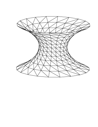
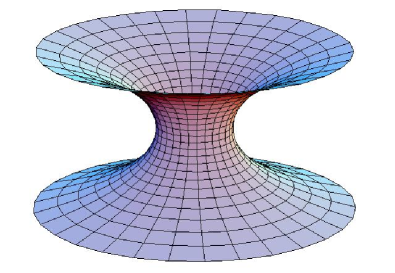
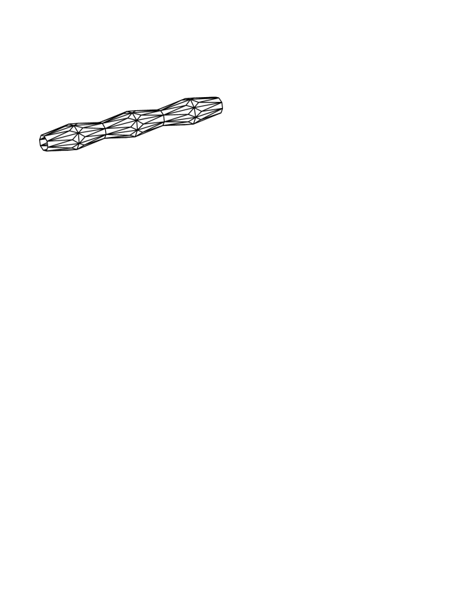
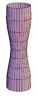
Figure 4. Discrete minimal catenoids and Delaunay surfaces. The example in the upper left (resp. lower left) is discrete minimal (resp. discrete CMC) with respect to the variational approach. The example in the upper right (resp. lower right) is discrete minimal (resp. discrete CMC) with respect to an integrable systems approach.

2. Smooth CMC surfaces and their variational properties

We defined mean curvature $H$ and CMC surfaces in [59]. The definition there states that surfaces for which $H$ is constant are CMC surfaces, and that minimal surfaces are those CMC surfaces with mean curvature $H=0$. In this section, we consider why, with these definitions, minimal and CMC surfaces are models for soap films.

The first and second variation formulas here are important for understanding how CMC and minimal surfaces are models for soap films, and in turn for understanding why we are interested in such surfaces. However, since these formulas will not be directly used later in this text, we content ourselves with stating them without proof, and with stating some other properties without proof as well. Furthermore, to simplify the discussion a bit, we restrict ourselves in this section to the case that the ambient space is $\mathbb{R}^{3}$. (Analogous properties hold for the minimal and CMC surfaces in the other ambient spaces we consider, with slightly different formulas.)

Let

$$f:\Sigma\to\mathbb{R}^{3}$$

be an immersion of a $2$-dimensional domain $\Sigma$ in the $(u,v)$-plane $\mathbb{R}^{2}$ (i.e. the plane $\mathbb{R}^{2}$ with Cartesian coordinates $u$ and $v$) into $\mathbb{R}^{3}$ with induced metric $g$ and with unit normal vector $\vec{N}=\vec{N}(u,v)$. We first note that another equivalent way to define the mean curvature $H$ at $f(p)$ is as the average of the normal curvatures

$$-\langle\vec{v},D_{\vec{v}}\vec{N}\rangle$$

(intuitively, the normal curvature measures the rate at which the surface bends toward $\vec{N}$, in the direction $\vec{v}$) in all tangent directions

$$\vec{v}\in{\mathcal{S}}=\{\vec{w}\in T_{p}\Sigma\,|\,g(\vec{w},\vec{w})=1\}\;,$$

where the average is computed by integrating $-\langle\vec{v},D_{\vec{v}}\vec{N}\rangle$ over $\mathcal{S}$ (with respect to an appropriate $1$-dimensional volume form on $\mathcal{S}$, which we do not describe explicitly here). Thus, for example, a minimal surface has average normal curvature zero at every point, and this suggests a physical interpretation, for which we quote [76]:

[76]: “Loosely speaking, one imagines the surface as made up of very many rubber bands, stretched out in all directions; on a minimal surface the forces due to the rubber bands balance out, and the surface does not need to move to reduce tension.”

To say this more rigorously, suppose $\Sigma$ is a compact domain in the $(u,v)$-plane, and define a smooth boundary-fixing variation of the immersion $f(\Sigma)$ to be a $C^{\infty}$ map $f_{t}:(-1,1)\times\Sigma\to\mathbb{R}^{3}$ with three properties:

1. $f_{t}(\cdot):\Sigma\to\mathbb{R}^{3}$ is an immersion for all $t\in(-1,1)$,

2. $f_{0}=f$ on $\Sigma$,

3. $f_{t}|_{\partial\Sigma}=f|_{\partial\Sigma}$ for all $t\in(-1,1)$.

We call

$$\tfrac{d}{dt}f_{t}|_{t=0}$$

the variation vector field of $f_{t}$ at $t=0$.

Note that $\mbox{Area}(f_{t}(\Sigma))=\int_{\Sigma}dA_{t}$, where $dA_{t}=\sqrt{g_{t,11}g_{t,22}-g_{t,12}^{2}}dudv$ is the volume element (the area $2$-form) of the metric $g_{t}=(g_{t,ij})$ induced by the immersion $f_{t}$ with respect to the coordinates $(u,v)$ of $\Sigma$. It turns out that (see, for example, [112]) the first variation formula for smooth boundary-fixing variations is then

(2.1) $$\left.\frac{d}{dt}\mbox{Area}(f_{t}(\Sigma))\right|_{t=0}=-\int_{\Sigma}\left\langle H\vec{N},\left.\frac{d}{dt}f_{t}\right|_{t=0}\right\rangle dA_{0}\;.$$

In particular, minimal surfaces (with $H\equiv 0$) are critical for area amongst all smooth boundary-fixing variations on any compact domain $\Sigma$, and we could have defined them this way. Actually, when the subdomain $\bar{\Sigma}$ of $\Sigma$ is small enough, not only is $f(\bar{\Sigma})$ critical for area, it is also the unique least-area surface with boundary $f(\partial\bar{\Sigma})$, hence ”minimal” surface is a natural name for such surfaces. Indeed, minimal surfaces are a natural $2$-dimensional generalization of $1$-dimensional geodesics, because geodesic segments of sufficiently short length are the least-length paths from one endpoint of the segment to the other (see Section 1.1 of [59]). Furthermore, although longer geodesics might not be least-length between their endpoints, they are still always critical for length amongst all smooth variations of the path fixing the endpoints (again, see Section 1.1 of [59]). This is completely analogous to the variational properties of minimal surfaces.

Similarly, a nonminimal CMC surface could be defined as an immersion $f:\Sigma\to\mathbb{R}^{3}$ such that $f(\Sigma)$ is critical for area amongst all smooth boundary-fixing variations that keep the volume on one side of the surface unchanged: the derivative of this volume with respect to $t$, at $t=0$, is

$$\int_{\Sigma}\left\langle\vec{N},\left.\frac{d}{dt}f_{t}\right|_{t=0}\right\rangle dA_{t}\;,$$

so if the volume is unchanging with respect to $t$, and hence $\int_{\Sigma}\langle\vec{N},\left.\frac{d}{dt}f_{t}\right|_{t=0}\rangle dA_{t}=0$, and if $H$ is constant, then Equation (2.1) implies (also, see [8], for example)

$$\left.\frac{d}{dt}\mbox{Area}(f_{t}(\Sigma))\right|_{t=0}=0\;.$$

Variations that preserve volume to one side of $f_{t}|_{\Sigma}$ are called volume-preserving variations. This is a natural restriction to make for non-minimal CMC surfaces, as the example in item (2) of Section 1 shows. If the round sphere soap film described there were allowed to deform in a way that did not preserve the volume inside of it, it would reduce its area by simply reducing its radius, and shrink down to a single point with no area. But clearly this does not happen, and the reason it does not happen is because of this volume constraint.

We conclude that minimal surfaces in $\mathbb{R}^{3}$ are surfaces that are critical for area with respect to smooth variations that fix their boundaries, and CMC surfaces are critical for area with respect to smooth variations that fix their boundaries and fix the volume to one side of the surfaces. This is why minimal and CMC surfaces model physical soap films, which always move to minimize area. Minimal surfaces model soap films not enclosing bounded pockets of air, as such films are area minimizing for all boundary-fixing variations. Nonminimal CMC surfaces model soap films enclosing bounded pockets of air, as such films are area minimizing only for variations that keep the air pockets’ volumes fixed.

These variational properties in the Euclidean case similarly hold for other ambient spaces, such as $\mathbb{S}^{3}$ and $\mathbb{H}^{3}$ (see Section 3, see also [59]).

The second variation formula for volume-preserving variations of CMC surfaces ([7], [36], [158], [112]) is (we may ignore the volume-preserving condition when the CMC surface is minimal)

(2.2) $$\left.\frac{d^{2}}{dt^{2}}\text{Area}(f_{t}(\Sigma))\right|_{t=0}=\int_{\Sigma}h\cdot L(h)dA_{0}\;,$$

where

$$L(h)=-\triangle h-(4H^{2}-2K)h\;\;\text{ and }\;\;h=\langle\tfrac{d}{dt}f_{t}|_{t=0},\vec{N}|_{t=0}\rangle\;,$$

with Gaussian curvature $K$ (see [59]) and Laplace-Beltrami operator

$$\triangle h=\frac{1}{\mathfrak{G}}\left(\partial_{u}(\mathfrak{G}g^{11}\partial_{u}h)+\partial_{u}(\mathfrak{G}g^{12}\partial_{v}h)+\partial_{v}(\mathfrak{G}g^{21}\partial_{u}h)+\partial_{v}(\mathfrak{G}g^{22}\partial_{v}h)\right)\;,$$

where $\mathfrak{G}=\sqrt{g_{11}g_{22}-g_{12}^{2}}$, and $g^{-1}=(g^{ij})_{i,j=1,2}$ is the inverse matrix of $g=g_{0}=(g_{ij})_{i,j=1,2}$.

Since the first derivative $\tfrac{d}{dt}\text{Area}(f_{t}(\Sigma))|_{t=0}$ is zero for CMC surfaces with respect to the appropriate variations, the sign of the second derivative (2.2) determines whether a variation increases or decreases the area. If there exists a variation $f_{t}$ so that (2.2) becomes negative, then the minimal or CMC surface will not be area minimizing with respect to the appropriate space of variations. If, on the other hand, (2.2) is positive for every nontrivial variation $f_{t}$ with respect to the appropriate variation space, then the minimal or CMC surface will be locally area minimizing in the space of variations.

The four examples of soap films described at the beginning of Section 1 are examples of minimal and CMC surfaces that are area-minimizing. If they had not been area-minimizing we never would have been able to construct them with soap films in the first place. However, not all of these four examples extend (analytically) to larger CMC surfaces that are area-minimizing (even though any CMC extensions are certainly still area-critical, by the first variation formula (2.1)). The first example, the flat disk, can be extended to a complete flat plane, which is a minimal surface. The complete flat plane is area-minimizing in the sense that any compact region $\Sigma$ within it is area-minimizing (with respect to the compact region’s boundary) and can be made as a soap film with a planar wire frame in the shape of its boundary. In particular, (2.2) will always be positive for any nontrivial smooth boundary fixing variation of any such compact region $\Sigma$. The second example, the round sphere, is already complete and so cannot be extended at all.

It is the third and fourth examples that extend to surfaces which are not area-minimizing. Let us consider the fourth example first. The fourth example is a round cylinder, and, up to a rigid motion of $\mathbb{R}^{3}$, we can represent it by the immersion

$$f(u,v)=(r\,\cos u,r\,\sin u,r\,v)$$

for $(u,v)\in\Sigma=[0,2\pi]\times[0,\tfrac{d}{r}]\subset\mathbb{R}^{2}$ for some constants $r,d\in\mathbb{R}^{+}$. This is a portion of a cylinder with radius $r$ and height $d$. The induced fundamental forms (see [59]) are

$$g=r^{2}dzd\bar{z}\;\;\;\text{ and }\;\;\;b=-\tfrac{r}{4}dz^{2}-\tfrac{r}{2}dzd\bar{z}-\tfrac{r}{4}d\bar{z}^{2}\;,\;\;\;\text{with}\;\;\;z=u+iv\;,\;\;\;i=\sqrt{-1}\;.$$

So $K=0$ and $H=\frac{-1}{2r}$, and the right-hand side of (2.2) is

(2.3) $$\int_{0}^{\tfrac{d}{r}}\int_{0}^{2\pi}h\cdot L_{cyl}(h)dudv\;,\;\;\;\;\;\;L_{cyl}(h)=-h_{uu}-h_{vv}-h\;.$$

This second derivative of area can be negative for some boundary-fixing volume-preserving variation if and only if $d>2\pi r$, and there is a reason why $2\pi r$ is the height beyond which the cylinder becomes only area-critical instead of area-minimizing. We will not fully explain the reason here (we refer the reader to [7] for a rigorous explanation), but we will give a clue as to why this is so. Consider the function

$$h=h(v)=\sin\tfrac{2\pi rv}{d}\;.$$

It has these properties:

• $h|_{v=0}=h|_{v=d/r}=0$ (an infinitesimal ”boundary-fixing” property),

• $\int_{0}^{d/r}hdv=0$ (an infinitesimal ”volume-preserving” property),

• $L_{cyl}(h)=\mu h$, where

  $$\mu=\frac{4\pi^{2}r^{2}-d^{2}}{d^{2}}\;.$$

Thus $h$ is an eigenfunction of the operator $L_{cyl}$ with eigenvalue $\mu$, and $\mu<0$ precisely when $d>2\pi r$. So if we choose a rotationally symmetric variation based on this function $h$ (i.e. a rotationally symmetric variation whose variation vector field at $t=0$ is $h\cdot\vec{N}$, where $\vec{N}=(\cos u,\sin u,0)$ is the unit normal vector to $f=f(u,v)$, see [7]), the integrand in the second variation formula (2.3) will become negative precisely when $d>2\pi r$. We conclude that a cylindrical tube of radius $r$ and height $d>2\pi r$ cannot be made as a physical film.

The third example of a soap film from Section 1 is a catenoid. The profile curve for a catenoid is the hyperbolic cosine function, so a catenoid can be parametrized as

$$f(u,v)=(\cosh v\cos u,\cosh v\sin u,v)\;,$$

with

$$(u,v)\in\Sigma=[0,2\pi]\times[-d,d]\subset\mathbb{R}^{2}$$

for some $d\in\mathbb{R}^{+}$. Here $2d$ is the distance between the two boundary circles. Let $d_{0}\approx 1.2$ be the unique positive solution to $d_{0}\sinh d_{0}=\cosh d_{0}$. Then the catenoid $f$ will be area-minimizing if $d<d_{0}$ and will not be area-minimizing (i.e. only area-critical) if $d>d_{0}$. Hence if we extend the value $d$ past $d_{0}$, the catenoid will no longer be constructable with a soap film.

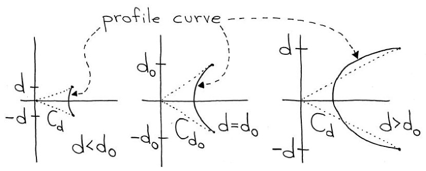
Figure 5. The profile curve on the left (resp. middle, right) creates a stable (resp. weakly stable, unstable) catenoid.

Again, we will not explain here why $d_{0}$ is the precise value beyond which the catenoid becomes non-area-minimizing, but, again, we will give a hint why this is so. The value $d_{0}$ actually has a geometric interpretation, as follows: For each $v>0$, consider the cone

$$C_{v}=\left\{\left.\left(x,y,\pm\frac{v}{\cosh v}\sqrt{x^{2}+y^{2}}\right)\,\right|\,x,y\in\mathbb{R}\right\}\;.$$

Then the cone $C_{v}$ intersects the catenoid tangentially (i.e. a non-transversal non-empty intersection) if and only if $v=d_{0}$. When $d<d_{0}$, any homothety of $\mathbb{R}^{3}$ centered at the origin $(0,0,0)$ will move the catenoid to another catenoid disjoint from the first one, while this is not the case when $d>d_{0}$. These facts are related to the question of whether there exists a boundary-fixing variation $f_{t}$ of the catenoid $f$ that has negative second derivative of area (we do not need the ”volume-preserving” property here, as the catenoid is a minimal surface). For a complete explanation of this, a good source is [37].

2.1. Steiner points

Minimal surfaces minimize area (at least locally) with respect to their boundary curves, thus, as noted above, they model soap films that do not surround bounded pockets of air. One could consider the analogous phenonemon, but one dimension lower. Instead of trying to connect $1$-dimensional things like sets of curves (i.e. the wire frames that we use to make soap bubbles) with area-minimizing surfaces, we could try to connect $0$-dimensional things such as finite sets of points, and instead of connecting them with $2$-dimensional surfaces, we would connect them with $1$-dimensional curves, and instead of trying to minimize the areas of the $2$-dimensional surfaces, we would minimize lengths of the $1$-dimensional curves. As we saw in Figure 2, the area-minimizing soap films can have $1$-dimensional singular curves where three sheets of a soap film come together at equal angles. When the dimension is reduced by $1$ as above, the singular curves are replaced with Steiner points, which are singular points at which three curves (actually straight line segments) come together at equal angles.

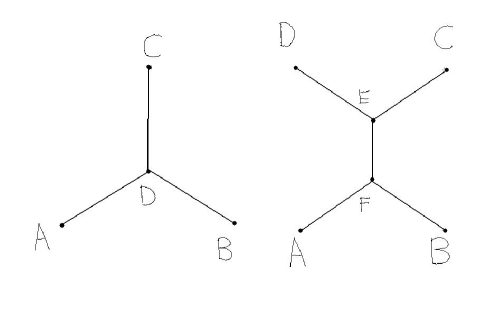
Figure 6. Examples of Steiner points in length-minimizing planar graphs.

To demonstrate this, let us consider the following examples:

Example 2.1.

Imagine you have two cities, call them city $A$ and city $B$, on a flat region of land, where no mountains or lakes or other obstructions exist, and you want to build a road (or collection of roads) that connects the two cities. Suppose further that you want to minimize the total length of the road (or roads).

You would, of course, just build one road along the straight line from city $A$ to city $B$. (The mathematicial statement would be that the shortest path between two points is a straight line.)

Example 2.2.

Now imagine that there are three cities, city $A$, city $B$ and city $C$, and that those three cities lie at the three vertices of an equilateral triangle. Now you want to build roads with minimal total length so that all three cities are connected, i.e. so that you can drive from any one city to any other of the three.

Suppose that the length of each side of the triangle is $\ell$. If you just build a straight road from city $A$ to city $B$, and another straight road from city $A$ to city $C$, then you would not need to build any road from city $B$ to city $C$, as you could already get from city $B$ to city $C$ by passing through city $A$. The total length of the roads would be $2\ell$.

But this is not actually the best solution. The best way is to make a new city $D$ at the center of the triangle, and then make three straight-line roads, one from each of the cities $A$, $B$ and $C$ directly to city $D$. Now the sum of the three lengths of these roads would be $\sqrt{3}\ell$, which is strictly less than $2\ell$, and this is the best way. See Figure 6.

The city $D$ in the previous example is what we call a Steiner point. It is an added point that is used to minimize total length of roads.

Example 2.3.

Now imagine that you have four cities, cities $A$, $B$, $C$ and $D$, at the vertices of a square with sides of length $\ell$, in sequencial order around the square. To connect these four cities so that the road length is minimized, you might first think of building three straight-line roads, each of length $\ell$, one from city $A$ to city $B$, one from city $B$ to city $C$ and one from city $C$ to city $D$. (Note that you now do not need a road from city $A$ to city $D$, just as in the previous example). Then the total length of roads is $3\ell$.

But this is not the best way. A better way would be to put a city $E$ at the center of the square and draw roads directly from each of the four original cities to the new city $E$. Then the roads form an ”X” and the length is now $2\sqrt{2}\ell$, which is less.

But this is still not the best solution. The best solution is to actually have two new cities $E$ and $F$ (i.e. two Steiner points), and then to draw in roads as in the second picture of Figure 6. The two Steiner points are placed in this picture so that the angle between any two roads meeting at a Steiner point is always exactly 120 degrees. One can now check the total length of the roads is strictly less than $2\sqrt{2}\ell$, and this is the best solution. Note that there are two different ways to choose a least-length solution.

In the above three examples, we have seen how Steiner points help us to find the least-length collection of ”1-dimensional” curves (i.e. roads) that connects some points (cities) together. This is analogous to the way singular points (and singular curves) can appear on area-minimizing surfaces.

3. Ambient spaces

CMC surfaces always exist in some larger ambient space. In the soap-film examples we described in Chapters 1 and 2, we were assuming that the CMC surfaces lie in the Euclidean $3$-space $\mathbb{R}^{3}$. We encountered CMC surfaces in other non-Euclidean ambient spaces in [59]. Also, there is a description of general Riemannian and Lorentzian manifolds in [59]. Here we give two examples of ambient spaces: we describe hyperbolic 3-space, like in [59], but in a bit more detail; we also briefly describe de Sitter $3$-space. Minkowski ($n+1$)-space $\mathbb{R}^{n,1}$ and spherical $3$-space $\mathbb{S}^{3}$ also appear in these notes, and we assume the reader is already familiar with those spaces (they are described in [59]).

3.1. Hyperbolic $3$-space $\mathbb{H}^{3}$

Hyperbolic $3$-space $\mathbb{H}^{3}$ is the unique simply-connected $3$-dimensional complete Riemannian manifold with constant sectional curvature $-1$. However, it can be described by a variety of models, each with its own advantages: the Minkowski space model, the Poincare ball model, the Hermitian matrix model, the Klein ball model and the upper-half-space model.

We define $\mathbb{H}^{3}$ by way of the Minkowski $4$-space $\mathbb{R}^{3,1}$ with its Lorentzian metric $g_{\mathbb{R}^{3,1}}$ of signature $(+++-)$, by taking the upper sheet of the two-sheeted hyperboloid

$$\mathfrak{M}=\left\{(x_{1},x_{2},x_{3},x_{0})\in\mathbb{R}^{3,1}\,\left|\,x_{0}^{2}-\sum_{j=1}^{3}x_{j}^{2}=1\,,\;x_{0}>0\right.\right\}\;,$$

with metric $g$ given by the restriction of $g_{\mathbb{R}^{3,1}}$ to the tangent spaces of this $3$-dimensional upper sheet. We call this $\mathfrak{M}$ the Minkowski model for hyperbolic $3$-space. Although the metric $g=g_{\mathbb{R}^{3,1}}$ is Lorentzian and therefore not positive definite, the restriction of $g$ to this upper sheet is actually positive definite, so $\mathfrak{M}$ is a Riemannian manifold.

The isometry group of $\mathfrak{M}$ can be described using the matrix group

$$O_{+}(3,1)=\{A=(a_{ij})_{i,j=1}^{4}\in O(3,1)\,|\,a_{44}>0\}\;.$$

For $A\in O_{+}(3,1)$, the map

$$\mathbb{R}^{3,1}\ni\vec{x}\to(A(\vec{x})^{t})^{t}\in\mathbb{R}^{3,1}$$

is an isometry of $\mathbb{R}^{3,1}$ that preserves $\mathfrak{M}$, hence it is an isometry of $\mathfrak{M}$. In fact, all isometries of $\mathfrak{M}$ can be described this way.

The following lemma tells us that the Minkowski model for hyperbolic $3$-space is indeed the true hyperbolic $3$-space.

Lemma 3.1.

$\mathfrak{M}$ is a simply-connected $3$-dimensional complete Riemannian manifold with constant sectional curvature $-1$.

Since this lemma implies $\mathfrak{M}$ is really the hyperbolic $3$-space $\mathbb{H}^{3}$, we will in fact sometimes refer to this Minkowski space model $\mathfrak{M}$ simply as $\mathbb{H}^{3}$.

Proof.

It is clear that $\mathfrak{M}$ is simply-connected. Let us now check that it has constant sectional curvature $-1$.

For any point $p\in\mathfrak{M}$, there exists a matrix $A\in\text{SO}_{3}=O(3)\cap\{A\in M_{3\times 3}(\mathbb{R})\,|\,\det A=+1\}$ such that the $4\times 4$ matrix

$$\begin{pmatrix}&&&0\\ &A&&0\\ &&&0\\ 0&0&0&1\end{pmatrix}\in O_{+}(3,1)$$

preserves $\mathfrak{M}$ and maps $p$ to a point of the form $(0,0,\sinh(s),\cosh(s))$, $s\in\mathbb{R}$. Then the matrix

$$\begin{pmatrix}1&0&0&0\\ 0&1&0&0\\ 0&0&\cosh(-s)&\sinh(-s)\\ 0&0&\sinh(-s)&\cosh(-s)\end{pmatrix}\in O_{+}(3,1)\;$$

is an isometry of $\mathbb{R}^{3,1}$ that preserves $\mathfrak{M}$ and maps the point $(0,0,\sinh(s),\cosh(s))$ to the point $(0,0,0,1)$. Thus one can move an arbitrary point of $\mathfrak{M}$ to the point $(0,0,0,1)$ by an isometry of $\mathfrak{M}$. Now, if ${\mathcal{V}}_{1},{\mathcal{V}}_{2}$ are any two $2$-dimensional subspaces of the $3$-dimensional tangent space $T_{(0,0,0,1)}(\mathfrak{M})$, there exists a matrix $A\in O_{+}(3,1)$ representing an isometry of $\mathfrak{M}$ fixing $(0,0,0,1)$ such that $d\psi_{(0,0,0,1)}({\mathcal{V}}_{1})={\mathcal{V}}_{2}$. Therefore this model has constant sectional curvature, by Lemma 1.1.6 in [59]. Thus to see that $\mathfrak{M}$ has constant sectional curvature $-1$, one need only check that this is the value of the sectional curvature of a single fixed $2$-dimensional subspace of $T_{(0,0,0,1)}(\mathfrak{M})$. This can be done using Equation (1.1.10) or Equation (1.1.14) in [59], and we leave this computation to the reader.

Finally, we argue that $\mathfrak{M}$ is complete. Intersecting $\mathfrak{M}$ with the plane $\{x_{1}=x_{2}=0\}$, we obtain a curve that can be parametrized with unit speed by $\alpha(s)=(0,0,\sinh(s),\cosh(s))$, i.e. this parametrization is unit speed with respect to the metric $g$ of $\mathfrak{M}$. Since the domain of $\alpha(s)$ is all $s\in\mathbb{R}$, this curve $\alpha(s)$ is complete. And since any geodesic segment in $\mathfrak{M}$ can be moved by an isometry to $\alpha(s),\;0\leq s\leq a$ for some value of $a$, we know that any geodesic segment can be extended to a geodesic of infinite length. Therefore $\mathfrak{M}$ is complete. This completes the proof of the lemma. ∎

Remark 3.2.

In fact, the functions $\sinh(s)$ and $\cosh(s)$ can be defined by the condition that the curve $\alpha(s)=(0,0,\sinh(s),\cosh(s))$ with $\alpha(0)=(0,0,0,1)$ and $\frac{d\alpha}{ds}(0)=(0,0,1,0)$ is a unit-speed geodesic with respect to the metric $g$ of $\mathfrak{M}=\mathbb{H}^{3}$. This condition implies that the curve $\alpha(s)$ satisfies $x_{3}^{2}-x_{0}^{2}=-1$, so $\cosh^{2}(s)-\sinh^{2}(s)=1$, and by differentiation of $x_{3}^{2}-x_{0}^{2}=-1$ with respect to $s$ we have

$$\frac{\tfrac{dx_{0}}{ds}}{\tfrac{dx_{3}}{ds}}=\frac{x_{3}}{x_{0}}\Longrightarrow\frac{\tfrac{d}{ds}(\cosh(s))}{\tfrac{d}{ds}(\sinh(s))}=\frac{\sinh(s)}{\cosh(s)}\;.$$

Since $|\alpha^{\prime}(s)|^{2}=(\frac{dx_{3}}{ds})^{2}-(\frac{dx_{0}}{ds})^{2}=1$, it follows that

$$\frac{d}{ds}(\sinh(s))=\cosh(s)\;,\;\;\;\frac{d}{ds}(\cosh(s))=\sinh(s)\;.$$

Now that we know how to differentiate $\cosh(s)$ and $\sinh(s)$, we know the power series expansions of these functions about $s=0$. Comparing these series with the power series expansions for $e^{s}$ and $e^{-s}$ about $s=0$, we conclude that

$$\cosh(s)=\frac{e^{s}+e^{-s}}{2}\;,\;\;\;\sinh(s)=\frac{e^{s}-e^{-s}}{2}\;,$$

which of course are the standard definitions of $\cosh(s)$ and $\sinh(s)$. (An analogous analysis can be carried out for the sine and cosine functions on the unit circle in the Euclidean plane, viewing that unit circle as a geodesic in the unit sphere $\mathbb{S}^{2}$ in the natural extension of $\mathbb{R}^{2}$ to $\mathbb{R}^{3}$.)

Because the isometry group of $\mathfrak{M}$, which we have noted we may call simply $\mathbb{H}^{3}$, is the matrix group $O_{+}(3,1)$, the image of the geodesic $\alpha(t)=(0,0,\cosh t,\sinh t)$ under an isometry of $\mathbb{H}^{3}$ always lies in a $2$-dimensional plane of $\mathbb{R}^{3,1}$ containing the origin. Thus we can conclude that the image of any geodesic in $\mathbb{H}^{3}$ is formed by the intersection of $\mathbb{H}^{3}$ with a $2$-dimensional plane in $\mathbb{R}^{3,1}$ which passes through the origin $(0,0,0,0)$ of $\mathbb{R}^{3,1}$.

The Minkowski model is perhaps the best model of $\mathbb{H}^{3}$ for understanding the isometries and geodesics of $\mathbb{H}^{3}$. However, since the Minkowski model lies in the $4$-dimensional space $\mathbb{R}^{3,1}$, we cannot use it to view graphics of surfaces in $\mathbb{H}^{3}$. So we would like to have models that can be viewed on the printed page. We would also like to have a model that uses $2\times 2$ matrices to describe $\mathbb{H}^{3}$, as this is more compatible with the DPW method described in [59], and the discussion in Sections 12.4 and 12.5 here. With this in mind, we now give some other possible models for $\mathbb{H}^{3}$.

3.2. The Klein model

Let $\mathcal{K}$ be the $3$-dimensional ball in $\mathbb{R}^{3,1}$ lying in the hyperplane $\{x_{0}=1\}$ with radius $1$ and center at $(0,0,0,1)$. By Euclidean stereographic projection from the origin $(0,0,0,0)\in\mathbb{R}^{3,1}$ of the Minkowski model $\mathfrak{M}$ for $\mathbb{H}^{3}$ to $\mathcal{K}$, one has the Klein model $\mathcal{K}$ for $\mathbb{H}^{3}$. $\mathcal{K}$ is given the metric that makes this stereographic projection an isometry. Since the geodesics of $\mathbb{H}^{3}$ in the Minkowski model are formed by the intersections of $\mathbb{H}^{3}$ with $2$-dimensional planes in $\mathbb{R}^{3,1}$ which pass through the origin, it is clear that after projection to $\mathcal{K}$, the geodesics become Euclidean straight lines in the Klein model, and this is the advantage of the Klein model. However, the disadvantage of the Klein model is that its metric is not conformal to the Euclidean metric (we defined conformality in [59], and we also define it here in Definition 4.4).

3.3. The Poincare model

Let $\mathcal{P}$ be the $3$-dimensional ball in $\mathbb{R}^{3,1}$ lying in the hyperplane $\{x_{0}=0\}$ with radius $1$ and center at the origin $(0,0,0,0)$. By Euclidean stereographic projection from the point $(0,0,0,-1)\in\mathbb{R}^{3,1}$ of the Minkowski model for $\mathbb{H}^{3}$ to $\mathcal{P}$, one has the Poincare model $\mathcal{P}$ for $\mathbb{H}^{3}$. This stereographic projection is

(3.1) $$(x_{1},x_{2},x_{3},x_{0})\in\mathbb{H}^{3}\to\left(\frac{x_{1}}{1+x_{0}},\frac{x_{2}}{1+x_{0}},\frac{x_{3}}{1+x_{0}},0\right)\in\mathcal{P}\;.$$

$\mathcal{P}$ is given the metric $g$ that makes this stereographic projection an isomety. Since the fourth coordinate is identically zero in the Poincare model, we can simply remove it and view the Poincare model as the Euclidean unit ball

$$B^{3}=\{(x_{1},x_{2},x_{3})\in\mathbb{R}^{3}\;|\;\;x_{1}^{2}+x_{2}^{2}+x_{3}^{2}<1\}$$

in $\mathbb{R}^{3}$. One can compute that the metric

(3.2) $$g=\left(\frac{2}{1-x_{1}^{2}-x_{2}^{2}-x_{3}^{2}}\right)^{2}(dx_{1}^{2}+dx_{2}^{2}+dx_{3}^{2})$$

is the one that will make the stereographic projection (3.1) an isometry. By either Equation (1.1.10) or (1.1.14) in [59], the sectional curvature is constantly $-1$. This metric $g$ in (3.2) is written as a function times the Euclidean metric $dx_{1}^{2}+dx_{2}^{2}+dx_{3}^{2}$, and this means that the Poincare model’s metric is conformal to the Euclidean metric. From this it follows that angles between vectors in the tangent spaces are the same from the viewpoints of both the hyperbolic and Euclidean metrics, and this is why we prefer this model when showing graphics of surfaces in hyperbolic $3$-space. However, distances are clearly not Euclidean. In fact, the boundary

$$\partial B^{3}=\{(x_{1},x_{2},x_{3})\in\mathbb{R}^{3}\;|\;\;x_{1}^{2}+x_{2}^{2}+x_{3}^{2}=1\}$$

of the Poincare model is infinitely far from any point in $B^{3}$ with respect to the hyperbolic metric $g$ in (3.2). For example, consider the curve

$$c(t)=(t,0,0)\;,\;\;\;t\in[0,1)$$

in the Poincare model. Its length is

$$\int_{0}^{1}\sqrt{g(c^{\prime}(t),c^{\prime}(t))}dt=\int_{0}^{1}\tfrac{2dt}{1-t^{2}}=+\infty\;.$$

Thus the point $(0,0,0)$ is infinitely far from the boundary point $(1,0,0)$ in the Poincare model. For this reason, the boundary $\partial B^{3}$ is often called the ideal boundary at infinity.

Unlike the Klein model, geodesics in the Poincare model are not Euclidean straight lines. Instead they are segments of Euclidean lines and circles that intersect the ideal boundary $\partial B^{3}$ at right angles.

Important examples of surfaces in $\mathbb{H}^{3}$ are described in [59], using the Poincare ball model: totally geodesic hypersurfaces (also called hyperbolic planes), hyperspheres, spheres and horospheres.

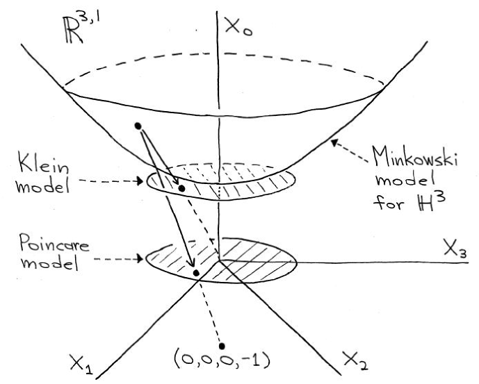
Figure 7. The Klein, Poincare and Minkowski space models for $\mathbb{H}^{3}$.

3.4. The upper-half-space model

One can obtain the upper-half-space model $\mathcal{U}$ for $\mathbb{H}^{3}$ from the Poincare model $\mathcal{P}$ by the Möbius transformation of $\mathbb{R}^{3}$ which maps the unit ball $B^{3}$ (with the Poincare metric) centered at the origin to the upper half $\{x_{3}>0\}$ of $\mathbb{R}^{3}$ and maps the origin $(0,0,0)$ to $(0,0,1)$ and fixes $\partial B^{3}\cap\{x_{3}=0\}$. This map is

$$\mathcal{P}\ni(x_{1},x_{2},x_{3})\to\frac{(2x_{1},2x_{2},1-x_{1}^{2}-x_{2}^{2}-x_{3}^{2})}{x_{1}^{2}+x_{2}^{2}+(x_{3}-1)^{2}}\in\mathcal{U}\;.$$

The metric induced on the upper-half-space by this transformation is

$$g=\frac{1}{x^{2}_{3}}(dx_{1}^{2}+dx_{2}^{2}+dx_{3}^{2})\;,$$

where we now view $(x_{1},x_{2},x_{3})$ as coordinates of the model $\mathcal{U}$, i.e. $x_{1},x_{2}\in\mathbb{R}$ and $x_{3}>0$. Thus, like the Poincare model, the upper-half space model $\mathcal{U}$ is again conformal to Euclidean space. And because Möbius transformations preserve angles and also the set of circles and lines, again the geodesics are Euclidean lines and circles that intersect the ideal boundary at infinity $\{x_{3}=0\}$ at right angles. The isometries of the model $\mathcal{U}$ are generated by horizontal Euclidean translations, Euclidean rotations about vertical axes, Euclidean dilations about points in the plane $\{x_{3}=0\}$, and Euclidean inversions through Euclidean spheres (and planes) intersecting the plane $\{x_{3}=0\}$ orthogonally.

3.5. The Hermitian matrix model

The Hermitian matrix model is a convenient model for applying the DPW method. Unlike the other four models above, which can be used for hyperbolic spaces of any dimension, the Hermitian model can be used only when the hyperbolic space is $3$-dimensional.

We first recall the following definitions: The group $\operatorname{SL}_{2}\!\mathbb{C}$ is all $2\times 2$ matrices with complex entries and determinant $1$, with matrix multiplication as the group operation. The vector space $\operatorname{sl}_{2}\!\mathbb{C}$ consists of all $2\times 2$ complex matrices with trace $0$, with the vector space operations being matrix addition and scalar multiplication. (In Section 3.7 we will see that $\operatorname{SL}_{2}\!\mathbb{C}$ is a Lie group. $\operatorname{SL}_{2}\!\mathbb{C}$ is $6$-dimensional. Also, $\operatorname{sl}_{2}\!\mathbb{C}$ is the associated Lie algebra, thus is the tangent space of $\operatorname{SL}_{2}\!\mathbb{C}$ at the identity matrix. $\operatorname{sl}_{2}\!\mathbb{C}$ is also $6$-dimensional.) The group $\operatorname{SU}_{2}$ is the subgroup of matrices $F\in\operatorname{SL}_{2}\!\mathbb{C}$ such that $F\cdot F^{*}$ is the identity matrix, where $F^{*}=\bar{F}^{t}$. Equivalently,

$$F=\left(\begin{array}[]{cc}p&-\bar{q}\\ q&\bar{p}\end{array}\right)\;,$$

for some $p$, $q\in\mathbb{C}$ with $|p|^{2}+|q|^{2}=1$. (We will see that $\operatorname{SU}_{2}$ is a $3$-dimensional Lie subgroup, in Section 3.7.)

Finally, we define Hermitian symmetric matrices as matrices of the form

$$\left(\begin{array}[]{cc}a_{11}&a_{12}\\ \overline{a_{12}}&a_{22}\end{array}\right)\;,$$

where $a_{12}\in\mathbb{C}$ and $a_{11},a_{22}\in\mathbb{R}$. Hermitian symmetric matrices with determinant $1$ have the additional condition that $a_{11}a_{22}-a_{12}\overline{a_{12}}=1$.

The Minkowski $4$-space $\mathbb{R}^{3,1}$ can be mapped to the space of $2\times 2$ Hermitian symmetric matrices by

$$\psi:(x_{1},x_{2},x_{3},x_{0})\longrightarrow\left(\begin{array}[]{cc}x_{0}+x_{3}&x_{1}+ix_{2}\\ x_{1}-ix_{2}&x_{0}-x_{3}\end{array}\right)\;.$$

For $\vec{x}\in\mathbb{R}^{3,1}$, the metric in the Hermitean matrix form is given by

$$\langle\vec{x},\vec{x}\rangle_{\mathbb{R}^{3,1}}=-\mbox{det}(\psi(\vec{x}))\;.$$

Thus $\psi$ maps the Minkowski model for $\mathbb{H}^{3}$ to the set of Hermitian symmetric matrices with determinant $1$. Any Hermitian symmetric matrix with determinant $1$ can be written as the product $FF^{*}$ for some $F\in\operatorname{SL}_{2}\!\mathbb{C}$, and $F$ is determined uniquely up to right-multiplication by elements in $\operatorname{SU}_{2}$. That is, for $F,\hat{F}\in\operatorname{SL}_{2}\!\mathbb{C}$, we have $FF^{*}=\hat{F}\hat{F}^{*}$ if and only if $F=\hat{F}\cdot B$ for some $B\in\operatorname{SU}_{2}$. Therefore we have the Hermitian model

$${\mathcal{H}}=\{FF^{*}\;|\;F\in\operatorname{SL}_{2}\!\mathbb{C}\}\;,\;\;\;\;\;F^{*}:=\bar{F}^{t}\;,$$

for $\mathbb{H}^{3}$, and $\mathcal{H}$ is given the metric so that $\psi$ is an isometry from the Minkowski model of $\mathbb{H}^{3}$ to $\mathcal{H}$.

It follows that, when we compare the Hermitean matrix and Poincare models $\mathcal{H}$ and $\mathcal{P}$ for $\mathbb{H}^{3}$, the mapping

$$\left(\begin{array}[]{cc}a_{11}&a_{12}\\ \overline{a_{12}}&a_{22}\end{array}\right)\in{\mathcal{H}}\to\left(\frac{a_{12}+\overline{a_{12}}}{2+a_{11}+a_{22}},\frac{i(\overline{a_{12}}-a_{12})}{2+a_{11}+a_{22}},\frac{a_{11}-a_{22}}{2+a_{11}+a_{22}}\right)\in{\mathcal{P}}$$

is an isometry from $\mathcal{H}$ to $\mathcal{P}$.

The Hermitian model is actually very convenient for describing the isometries of $\mathbb{H}^{3}$. Up to scalar multiplication by $\pm 1$, the group $\operatorname{SL}_{2}\!\mathbb{C}$ represents the isometry group of $\mathbb{H}^{3}$ in the Hermitian model $\mathcal{H}$ in the following way: A matrix $h\in\operatorname{SL}_{2}\!\mathbb{C}$ acts isometrically on $\mathbb{H}^{3}$ in the model $\mathcal{H}$ by

$$x\in\mathcal{H}\to h\cdot x:=h\,x\,h^{*}\in\mathcal{H}\;,$$

where $h^{*}=\bar{h}^{t}$. The kernel of this action is $\pm I$, hence $\operatorname{PSL}_{2}\!\mathbb{C}=\operatorname{SL}_{2}\!\mathbb{C}/\{\pm I\}$ is the isometry group of $\mathbb{H}^{3}$.

3.6. De-Sitter $3$-space $\mathbb{S}^{2,1}$

Finally, we briefly consider another ambient space, which will be a Lorentzian manifold, because it also has a $2\times 2$ Hermitian matrix model. Consider the $1$-sheeted hyperboloid in $\mathbb{R}^{3,1}$

$$\mathbb{S}^{2,1}=\left\{(x_{1},x_{2},x_{3},x_{0})\in\mathbb{R}^{3,1}\,\left|\,\sum_{j=1}^{3}x_{j}^{2}-x_{0}^{2}=1\right.\right\}$$

with the metric $g$ induced on its tangent spaces by the restriction of the metric from the Minkowski space $\mathbb{R}^{3,1}$. This Lorentzian manifold $\mathbb{S}^{2,1}$ is called de-Sitter $3$-space.

De-Sitter $3$-space $\mathbb{S}^{2,1}$ is homeomorphic to $\mathbb{S}^{2}\times\mathbb{R}$, so it is simply-connected, since both $\mathbb{S}^{2}$ and $\mathbb{R}$ are individually simply-connected. And this space, like hyperbolic space $\mathbb{H}^{3}$, can also be written with a $2\times 2$ matrix model:

$$\mathbb{S}^{2,1}=\left\{X\in M_{2\times 2}(\mathbb{C})\,|\,X^{*}=X,\langle X,X\rangle_{\mathbb{R}^{3,1}}=1\right\}=\left\{\left.F\begin{pmatrix}1&0\\ 0&-1\end{pmatrix}F^{*}\,\right|\,F\in\operatorname{SL}_{2}\!\mathbb{C}\right\}\;,$$

where $\langle X,X\rangle_{\mathbb{R}^{3,1}}=-\det X$. We note that $\mathbb{S}^{2,1}$ has constant sectional curvature $+1$.

3.7. Lie groups and algebras

We have already seen some Lie groups, that are amongst the most basic matrix groups, so here we briefly review some basic facts about Lie groups and algebras.

Definition 3.3.

A set $G$ is a Lie group if

1. $G$ is a differentiable manifold of class $C^{\infty}$,

2. $G$ is a group with respect to some group operation, denoted by $\cdot$,

3. for each fixed $g_{0}\in G$ and each variable $g\in G$, the maps $L_{g_{0}}:g\to g_{0}\cdot g$ (left multiplication) and $R_{g_{0}}:g\to g\cdot g_{0}$ (right multiplication) are $C^{\infty}$ differentiable.

Definition 3.4.

The Lie algebra $\mathfrak{G}$ associated to a Lie group $G$ is the tangent space of (the manifold) $G$ at the identity element $e$ of (the group) $G$, i.e. $\mathfrak{G}=T_{e}G$. The Lie algebra $\mathfrak{G}$ is then a vector space under addition and scalar multiplication of vectors in $T_{e}G$. Furthermore, there is a bracket operation $\mathfrak{G}\times\mathfrak{G}\to\mathfrak{G}$ defined as follows:

$$[X,Y](f)=X(Y(f))-Y(X(f))\;,$$

where $X,Y$ are arbitrary elements of $\mathfrak{G}$ with canonical left-invariant extensions to vector fields on $G$, and $f:G\to\mathbb{R}$ is any smooth map.

Remark 3.5.

$X$ being a left-invariant vector field means that $X$ is given by transportation by the derivative map of left multiplication in $G$, i.e.

$$X_{g}=(L_{g})_{*}X_{e}\;,$$

where $L_{g}:G\to G$ denotes left multiplication by $g$, as in part (3) of Definition 3.3. In the case that $G$ is a matrix group, then $(L_{g})_{*}X$ becomes simply $(L_{g})_{*}X=gX$, and the above equation can be written as $X_{g}=gX_{e}$.

Remark 3.6.

In the definition of the Lie bracket above, $X(f)$ and $Y(f)$ must be defined at more than just one point $e$ (in particular, in a neighborhood of $e$) in order for $Y(X(f))$ and $X(Y(f))$ to be defined. But because we take the canonical left-invariant extensions of $X$ and $Y$, in fact $[X,Y]$ is determined by $X|_{e}$ and $Y|_{e}$ alone.

Remark 3.7.

When $G$ is a matrix group, $X$ and $Y$ in $\mathfrak{G}$ can be identified with matrices, and it turns out that $[X,Y]$ can be identified with the difference of matrix products $X\cdot Y-Y\cdot X$. We will give an example of this in Example 3.11.

Example 3.8.

The first example we consider is $\text{SO}_{3}$, defined as follows:

$$\text{SO}_{3}=\{A\in M_{3\times 3}(\mathbb{R})\,|A\cdot A^{t}=I,\,\det A=1\}\;.$$

The group operation is then matrix multiplication. This represents the group of rotations of $\mathbb{R}^{3}$ that fix the origin of $\mathbb{R}^{3}$, and the group operation then represents composition of rotations. When considering a conformal immersion $f:\Sigma\to\mathbb{R}^{3}$ defined on a $2$-dimensional Riemann surface $\Sigma$ with local coordinate $z=u+iv$, we can consider the three vectors (two being tangent to $f$, and the third being the unit normal vector to $f$)

$$\tfrac{f_{u}}{||f_{u}||}|_{f(p)}\;,\;\;\tfrac{f_{v}}{||f_{v}||}|_{f(p)}\;,\;\;\vec{N}|_{f(p)}$$

to be an orthonormal frame of $T_{f(p)}\mathbb{R}^{3}$. We can use an element of $\text{SO}_{3}$ to describe this orthonormal frame by choosing the unique element of $\text{SO}_{3}$ that rotates $(1,0,0)$ and $(0,1,0)$ and $(0,0,1)$ to $\tfrac{f_{u}}{||f_{u}||}|_{f(p)}$ and $\tfrac{f_{v}}{||f_{v}||}|_{f(p)}$ and $\vec{N}|_{f(p)}$, respectively. We denote the Lie algebra of $\text{SO}_{3}$ by $so_{3}$.

Example 3.9.

The second example we consider is $\operatorname{SL}_{2}\!\mathbb{C}$, defined as follows:

$$\operatorname{SL}_{2}\!\mathbb{C}=\{A\in M_{2\times 2}(\mathbb{C})\,|\det A=1\}\;.$$

Again the group operation is matrix multiplication, and the group operation represents composition of linear maps of $\mathbb{C}^{2}$ to itself. In fact, $\operatorname{SL}_{2}\!\mathbb{C}$ is a double cover of $\text{SO}_{3}$, as we saw in Sections 2.4 and 3.2 in [59]. We denote the Lie algebra of $\operatorname{SL}_{2}\!\mathbb{C}$ by $\operatorname{sl}_{2}\!\mathbb{C}$.

Example 3.10.

Our third example is a subgroup of $\operatorname{SL}_{2}\!\mathbb{C}$:

$$\operatorname{SU}_{2}=\{A\in\operatorname{SL}_{2}\!\mathbb{C}\,|A\cdot\bar{A}^{t}=I\}$$

$$=\left\{\left.\begin{pmatrix}p&q\\ -\bar{q}&\bar{p}\end{pmatrix}\,\right|p,q\in\mathbb{C},p\bar{p}+q\bar{q}=1\right\}\;.$$

The corresponding Lie algebra is denoted $\operatorname{su}_{2}$, and we explicitly compute $\operatorname{su}_{2}$ here: Consider a curve $c(t):(-\epsilon,\epsilon)\to\operatorname{SU}_{2}$ given by

$$c(t)=\begin{pmatrix}p(t)&q(t)\\ -\overline{q}(t)&\overline{p}(t)\end{pmatrix}$$

with $c(0)=I$. Then, with $\prime$ denoting the derivative with respect to $t$,

$$c^{\prime}(0)=\begin{pmatrix}p^{\prime}(0)&q^{\prime}(0)\\ -\overline{q^{\prime}}(0)&\overline{p^{\prime}}(0)\end{pmatrix}$$

is an arbitrary element of $\operatorname{su}_{2}=T_{I}\operatorname{SU}_{2}$. In general, for any square matrix $\mathcal{A}$, we have $(\det\mathcal{A})^{\prime}=\text{trace}(\mathcal{A}^{\prime}\cdot\mathcal{A}^{-1})\det\mathcal{A}$ (see Lemma 3.12 below), so if $\det\mathcal{A}$ is identically $1$, then the trace of $\mathcal{A}^{\prime}\cdot\mathcal{A}^{-1}$ is $0$. This implies that $c^{\prime}(0)$ is trace-free. Then, because $p(0)=1$ and $q(0)=0$, the derivative with respect to $t$ of $p(t)\overline{p}(t)+q(t)\overline{q}(t)=1$ implies $p^{\prime}(0)\in i\mathbb{R}$. We conclude that $\operatorname{su}_{2}$ is the $3$-dimensional vector space

$$\operatorname{su}_{2}=\left\{\left.\frac{-i}{2}\begin{pmatrix}-x_{3}&x_{1}+ix_{2}\\ x_{1}-ix_{2}&x_{3}\end{pmatrix}\;\right|\;x_{1},x_{2},x_{3}\in\mathbb{R}\right\}\;,$$

which is isomorphic as a vector space to $\mathbb{R}^{3}$, and so $\operatorname{su}_{2}$ is a matrix model for $\mathbb{R}^{3}$.

Example 3.11.

Our fourth example $\operatorname{SL}_{2}\!\mathbb{R}$ is also a subgroup of $\operatorname{SL}_{2}\!\mathbb{C}$:

$$\operatorname{SL}_{2}\!\mathbb{R}=\{A\in M_{2\times 2}(\mathbb{R})\,|\det A=1\}\;,$$

with associated Lie algebra

$$\text{sl}_{2}\mathbb{R}=\{A\in M_{2\times 2}(\mathbb{R})\,|\text{tr}A=0\}\;.$$

We now explicitly describe the bracket operation on $\text{sl}_{2}\mathbb{R}$, in order to provide an example for the claim in Remark 3.7. To determine the bracket operation, take the three curves

$$c_{1}(t)=\begin{pmatrix}1-t&0\\ 0&(1-t)^{-1}\end{pmatrix}\;,\;\;\;c_{2}(t)=\begin{pmatrix}1&t\\ 0&1\end{pmatrix}\;,\;\;\;c_{3}(t)=\begin{pmatrix}1&0\\ t&1\end{pmatrix}$$

in $\operatorname{SL}_{2}\!\mathbb{R}$ through the identity matrix at $t=0$. To move these curves to other points of $\operatorname{SL}_{2}\!\mathbb{R}$, we use matrix multiplication on the left, i.e.

$$c_{j,a,b,d}=\begin{pmatrix}a&b\\ d&(1+bd)a^{-1}\end{pmatrix}\cdot c_{j}(t)$$

for $j=1,2,3$ and $a,b,d\in\mathbb{R}$. (For our purposes we may assume $a\neq 0$.) Now $a,b,d$ represent coordinates for a region of $\operatorname{SL}_{2}\!\mathbb{R}$ considered as a $3$-dimensional manifold. In fact, we could regard the coordinate chart $\phi$ to be defined by

$$\phi^{-1}\left(\begin{pmatrix}a&b\\ d&(1+bd)a^{-1}\end{pmatrix}\right)=(a,b,d)\;,$$

as a map from a region of $\mathbb{R}^{3}$ to a region of $\operatorname{SL}_{2}\!\mathbb{R}$. Now, for a function

$$f:\operatorname{SL}_{2}\!\mathbb{R}\to\mathbb{R}\;,$$

the composite maps

$$f\circ\phi(a(1-t),b(1-t)^{-1},d(1-t))\;,$$

$$f\circ\phi(a,at+b,d)\;,$$

$$f\circ\phi(a+bt,b,(1+bd)a^{-1}t+d)$$

equal, respectively,

$$f(c_{j,a,b,d}(t))$$

for $j=1,2,3$. Then, by the chain rule, we have

$$\left.\frac{d}{dt}f(c_{j,a,b,d}(t))\right|_{t=0}=\vec{v}_{c_{j,a,b,d}}(f\circ\phi(a,b,d))\;,$$

for the three resulting left-invariant vector fields

$$\vec{v}_{c_{1,a,b,d}}=-a\partial_{a}+b\partial_{b}-d\partial_{d}\;,$$

$$\vec{v}_{c_{2,a,b,d}}=a\partial_{b}\;,$$

$$\vec{v}_{c_{3,a,b,d}}=b\partial_{a}+(1+bd)a^{-1}\partial_{d}\;.$$

Thus

$$\vec{v}_{c_{1,a,b,d}}\circ\vec{v}_{c_{2,a,b,d}}-\vec{v}_{c_{2,a,b,d}}\circ\vec{v}_{c_{1,a,b,d}}=-2\vec{v}_{c_{2,a,b,d}}\;,$$

$$\vec{v}_{c_{1,a,b,d}}\circ\vec{v}_{c_{3,a,b,d}}-\vec{v}_{c_{3,a,b,d}}\circ\vec{v}_{c_{1,a,b,d}}=2\vec{v}_{c_{3,a,b,d}}\;,$$

$$\vec{v}_{c_{2,a,b,d}}\circ\vec{v}_{c_{3,a,b,d}}-\vec{v}_{c_{3,a,b,d}}\circ\vec{v}_{c_{2,a,b,d}}=-\vec{v}_{c_{1,a,b,d}}\;.$$

Correspondingly,

$$c^{\prime}_{1}(0)=\begin{pmatrix}-1&0\\ 0&1\end{pmatrix}\;,\;\;\;c^{\prime}_{2}(0)=\begin{pmatrix}0&1\\ 0&0\end{pmatrix}\;,\;\;\;c^{\prime}_{3}(0)=\begin{pmatrix}0&0\\ 1&0\end{pmatrix}\;,$$

and

$$c^{\prime}_{1}(0)c^{\prime}_{2}(0)-c^{\prime}_{2}(0)c^{\prime}_{1}(0)=-2c^{\prime}_{2}(0)\;,$$

$$c^{\prime}_{1}(0)c^{\prime}_{3}(0)-c^{\prime}_{3}(0)c^{\prime}_{1}(0)=2c^{\prime}_{3}(0)\;,$$

$$c^{\prime}_{2}(0)c^{\prime}_{3}(0)-c^{\prime}_{3}(0)c^{\prime}_{2}(0)=-c^{\prime}_{1}(0)\;.$$

Thus the behavior of the bracket on vector fields is exactly the same as the behavior of commutators of matrices in the Lie algebra. This is why we can use matrix multiplication to define the Lie bracket in the case of $\text{sl}_{2}\mathbb{R}$, and this is true for matrix Lie groups in general.

We now prove an equation we used in the third example above:

Lemma 3.12.

For any square matrix $\mathcal{A}\in M_{n\times n}(\mathbb{C})$ with $\det A\neq 0$ that depends smoothly on some parameter $t\in\mathbb{R}$, we have

(3.3) $$\tfrac{d}{dt}(\det\mathcal{A})=\text{trace}((\tfrac{d}{dt}\mathcal{A})\cdot\mathcal{A}^{-1})\det\mathcal{A}\;.$$

Lemma 3.12 is easily proven in the case that $n=2$. It is also easily seen for general $n$ when $\mathcal{A}$ is upper triangular. Furthermore, if $\mathcal{A}$ satisfies Equation (3.3), it is easily seen that the conjugation $P\cdot\mathcal{A}\cdot P^{-1}$ also satisfies Equation (3.3), for any $P\in M_{n\times n}(\mathbb{C})$ with $\det P\neq 0$ that depends smoothly on $t$. Because any square matrix can be conjugated into an upper triangular matrix (the Jordan canonical form), this provides a proof of Lemma 3.12.

One could also prove Lemma 3.12 by direct computation: Write $\mathcal{A}=(a_{ij})_{i,j=1}^{n}$. Then let $\mathcal{A}_{i,b_{1},...,b_{n}}:=\mathcal{A}|_{\{a_{i1}\to b_{1},...,a_{in}\to b_{n}\}}$ be the matrix with entries as in $\mathcal{A}$, except that the $i$’th row has been replaced with the row vector $(b_{1}\,...\,b_{n})$. Then

(3.4) $$\det(\mathcal{A}_{i,b_{1},...,b_{n}})=\sum_{j=1}^{n}\det(\mathcal{A}_{i,0,...,0,b_{j},0,...,0})=\sum_{j=1}^{n}b_{j}\tilde{a}_{ij}\;,$$

where $b_{j}$ is the value in the $ij$’th position of $\mathcal{A}_{i,0,...,0,b_{j},0,...,0}$, and where

$$\tilde{a}_{ij}=\det(\mathcal{A}_{i,0,...,0,1,0,...,0})$$

(again, $1$ is the value in the $ij$’th position of $\mathcal{A}_{i,0,...,0,1,0,...,0}$). Then, for any $k\in\{1,...,n\}$, we have ($\delta_{ki}$ is the Kronecker delta function)

$$\sum_{j=1}^{n}a_{kj}\tilde{a}_{ij}=\det(\mathcal{A}_{i,a_{k1},...,a_{kn}})=\delta_{ki}\cdot\det(\mathcal{A})\;.$$

Hence, for

$$\tilde{\mathcal{A}}:=(\tilde{a}_{ij})_{i,j=1}^{n}\;,$$

we have

$$\mathcal{A}\cdot\tilde{\mathcal{A}}^{t}=\det(\mathcal{A})\cdot I_{n\times n}\;.$$

So if $\mathcal{A}$ is regular, i.e. $\det(\mathcal{A})\neq 0$, then

$$\mathcal{A}^{-1}=\tfrac{1}{\det(\mathcal{A})}\tilde{\mathcal{A}}^{t}\;.$$

Thus we have

$$\text{tr}((\tfrac{d}{dt}\mathcal{A})\mathcal{A}^{-1})\cdot\det(\mathcal{A})=\text{tr}((\tfrac{d}{dt}\mathcal{A})\tfrac{1}{\det(\mathcal{A})}\tilde{\mathcal{A}}^{t})\cdot\det(\mathcal{A})=$$

$$\text{tr}((\tfrac{d}{dt}\mathcal{A})\tilde{\mathcal{A}}^{t})=\sum_{i=1}^{n}\sum_{j=1}^{n}\frac{da_{ij}}{dt}\tilde{a}_{ij}=$$

$$\sum_{i=1}^{n}\det(\mathcal{A}_{i,a^{\prime}_{i1},...,a^{\prime}_{in}})=\frac{d}{dt}(\det(\mathcal{A}))\;,\;\;\;a_{ij}^{\prime}:=\frac{da_{ij}}{dt}\;,$$

where the second to the last equality above follows from Equation (3.4), proving Lemma 3.12.

A third proof of this lemma can be given by using the following fact: If $A$ and $X$ are $n\times n$ matrices and $\epsilon$ is a real number close to zero, then

(3.5) $$A=I+\epsilon X+\mathcal{O}(\epsilon^{2})\;\;\text{implies}\;\;\det(A)=1+\epsilon\cdot\text{tr}X+\mathcal{O}(\epsilon^{2})\;.$$

The argument is as follows: Write the Taylor expansion of $\mathcal{A}(s)$ at the value $s=t$ as

$$\mathcal{A}(s)=\mathcal{A}(t)+(s-t)\mathcal{A}^{\prime}(t)+\mathcal{O}((s-t)^{2})\;.$$

Then

$$\mathcal{A}(s)(\mathcal{A}(t))^{-1}=I+(s-t)\mathcal{A}^{\prime}(t)(\mathcal{A}(t))^{-1}+\mathcal{O}((s-t)^{2})\;,$$

and (3.5) implies

$$\det(\mathcal{A}(s)(\mathcal{A}(t))^{-1})=1+(s-t)\cdot\text{tr}(\mathcal{A}^{\prime}(t)(\mathcal{A}(t))^{-1})+\mathcal{O}((s-t)^{2})\;.$$

Taking the derivative of this with respect to $s$ and then evaluating at $s=t$, we have

$$\frac{(\det(\mathcal{A}(s)))^{\prime}|_{s=t}}{\det(\mathcal{A}(t))}=\left.\left(\text{tr}(\mathcal{A}^{\prime}(t)(\mathcal{A}(t))^{-1})+\mathcal{O}(s-t)\right)\right|_{s=t}\;,$$

so

$$\frac{(\det(\mathcal{A}(t)))^{\prime}}{\det(\mathcal{A}(t))}=\text{trace}(\mathcal{A}^{\prime}(t)(\mathcal{A}(t))^{-1})\;,$$

proving Lemma 3.12.

4. Riemann surfaces and Hopf’s theorem

4.1. Riemann surfaces

When the dimension of a differentiable manifold $M$ is two, then we have some special properties. This is because the coordinate charts are maps from $\mathbb{R}^{2}$, and $\mathbb{R}^{2}$ can be thought of as the complex plane $\mathbb{C}\approx\mathbb{R}^{2}$. Thus we can consider the notion of holomorphic functions on $M$. This leads to the idea of Riemann surfaces and the beautiful theory associated with them. Part of the beauty of this theory is that Riemann surfaces can be described in a variety of different ways, but this is outside the scope of this text, and for our purposes it suffices to consider just two descriptions of Riemann surfaces.

To distinguish $2$-dimensional manifolds from other manifolds, we will often denote them by $\Sigma$ instead of $M$.

Suppose $\Sigma$ is a differentiable manifold of dimension $2$ with differentiable structure defined by a family

$$\{\,(U_{\alpha}\,,\,\phi_{\alpha}:U_{\alpha}\to\Sigma)\,\}$$

of coordinate charts. Let $(u_{\alpha},v_{\alpha})$ be the coordinates of $U_{\alpha}\subseteq\mathbb{R}^{2}$. If $W:=\phi_{\alpha}(U_{\alpha})\cup\phi_{\beta}(U_{\beta})\neq\emptyset$, then $u_{\beta},v_{\beta}$ can be viewed as functions of the variables $u_{\alpha},v_{\alpha}$ on $\phi_{\alpha}^{-1}(W)$ via the transition function $f_{\beta\alpha}=\phi_{\beta}^{-1}\circ\phi_{\alpha}:\phi_{\alpha}^{-1}(W)\to\phi_{\beta}^{-1}(W)$. Associating $U_{\alpha}\subseteq\mathbb{R}^{2}$ with the corresponding region of $\mathbb{C}$ by defining the complex coordinate

$$z_{\alpha}=u_{\alpha}+iv_{\alpha}$$

for each coordinate chart $(U_{\alpha},\phi_{\alpha})$, we can view $z_{\beta}$ as a function of $z_{\alpha}$ on $\phi_{\alpha}^{-1}(W)$. When $z_{\beta}$ is a holomorphic function of $z_{\alpha}$, we say that the transition function $f_{\beta\alpha}$ is holomorphic.

Definition 4.1.

A differentiable manifold $\Sigma$ of dimension $2$ with differentiable structure defined by a family $\{(U_{\alpha},\phi_{\alpha})\}$ of coordinate charts is a Riemann surface if the transition functions $f_{\beta\alpha}$ are all holomorphic. We then say that the family $\{(U_{\alpha},\phi_{\alpha})\}$ forms a complex structure on $\Sigma$.

The simplest example of a Riemann surface is $\mathbb{C}$ itself. In this case, we can choose a single coordinate $(U_{\alpha},\phi_{\alpha})$ to give the differential structure, where $U_{\alpha}=\mathbb{R}^{2}$ and $\phi_{\alpha}$ is the identity map. Then it is vacuously true that the transition functions are holomorphic.

Another example is the unit sphere $\mathbb{S}^{2}$ (in $\mathbb{R}^{3}$). The differential structure can be defined by a pair of stereographic projections, so we can use two coordinate neighborhoods $(U_{\alpha},\phi_{\alpha})$ and $(U_{\beta},\phi_{\beta})$ with $U_{\alpha}=U_{\beta}=\mathbb{R}^{2}$, and with $\phi_{\alpha}$ equal to the inverse of stereographic projection from the north pole $(0,0,1)$, and with $\phi_{\beta}$ equal to the inverse of stereographic projection from the south pole $(0,0,-1)$ composed with a reflection of $\mathbb{S}^{2}$ across a plane fixing both the north and south poles. Then the map $\phi_{\beta}^{-1}\circ\phi_{\alpha}$ is holomorphic, so $\mathbb{S}^{2}$ is a Riemann surface.

One property of Riemann surfaces is that they are always orientable. Before proving this, we first recall the definition of orientability. Given two differentiable functions $f,g$ from a $2$-dimensional differentiable manifold $\Sigma$ to $\mathbb{R}$, we define the wedge product of their differentials as follows: For a point $p\in\Sigma$ and $\vec{v},\vec{w}\in T_{p}\Sigma$,

$$df_{p}\wedge dg_{p}(\vec{v},\vec{w})=\frac{1}{2}(df_{p}(\vec{v})dg_{p}(\vec{w})-df_{p}(\vec{w})dg_{p}(\vec{v}))\;.$$

(Note that the wedge product defined here is not the same as the symmetric product defined in Section 1.1 of [59].) Then, for coordinate neighborhoods $(U_{\alpha},\phi_{\alpha})$ and $(U_{\beta},\phi_{\beta})$ such that $W:=\phi_{\alpha}(U_{\alpha})\cup\phi_{\beta}(U_{\beta})\neq\emptyset$, and naming the coordinates $(u_{\alpha},v_{\alpha})$ and $(u_{\beta},v_{\beta})$ on $\phi_{\alpha}^{-1}(W)$ and $\phi_{\beta}^{-1}(W)$, respectively, we say that $(U_{\alpha},\phi_{\alpha})$ and $(U_{\beta},\phi_{\beta})$ are oriented in the same way if

$$du_{\alpha}\wedge dv_{\alpha}=h_{\alpha\beta}du_{\beta}\wedge dv_{\beta}$$

for some positive function $h_{\alpha\beta}:\phi_{\alpha}^{-1}(W)\to\mathbb{R}^{+}$.

If the coordinate charts $\{(U_{\alpha},\phi_{\alpha})\}$ that comprise the differential structure of $\Sigma$ can be chosen so that they are all oriented the same way wherever they intersect, we say that the manifold $\Sigma$ is orientable, and the family $\{(U_{\alpha},\phi_{\alpha})\}$ is said to be oriented.

Lemma 4.2.

Any Riemann surface is orientable.

Proof.

Let $(U_{\alpha},\phi_{\alpha})$ and $(U_{\beta},\phi_{\beta})$ be two coordinate charts of a Riemann surface $\Sigma$ such that $W:=\phi_{\alpha}(U_{\alpha})\cap\phi_{\beta}(U_{\beta})\neq\emptyset$. Let $(u_{\alpha},v_{\alpha})$ and $(u_{\beta},v_{\beta})$ be the coordinates of $\phi_{\alpha}^{-1}(W)\subseteq\mathbb{R}^{2}$ and $\phi_{\beta}^{-1}(W)\subseteq\mathbb{R}^{2}$, respectively. Noting that the differentials of $z_{\alpha}$, $\bar{z}_{\alpha}$, $z_{\beta}$ and $\bar{z}_{\beta}$ satisfy

$$dz_{\alpha}=du_{\alpha}+idv_{\alpha}\;,\;\;\;d\bar{z}_{\alpha}=du_{\alpha}-idv_{\alpha}\;,$$

$$dz_{\beta}=du_{\beta}+idv_{\beta}\;,\;\;\;d\bar{z}_{\beta}=du_{\beta}-idv_{\beta}\;,$$

and also that, because $z_{\beta}$ is a holomorphic function of $z_{\alpha}$ on $\phi_{\alpha}^{-1}(W)$, the chain rule implies

$$dz_{\alpha}=\frac{dz_{\alpha}}{dz_{\beta}}dz_{\beta}\;,$$

we have

$$du_{\alpha}\wedge dv_{\alpha}=\tfrac{i}{2}dz_{\alpha}\wedge d\bar{z}_{\alpha}=\tfrac{i}{2}\left|\tfrac{dz_{\alpha}}{dz_{\beta}}\right|^{2}dz_{\beta}\wedge d\bar{z}_{\beta}=\left|\tfrac{dz_{\alpha}}{dz_{\beta}}\right|^{2}du_{\beta}\wedge dv_{\beta}\;.$$

Since $\left|\tfrac{dz_{\alpha}}{dz_{\beta}}\right|^{2}>0$ for all $\alpha$ and $\beta$, we conclude that $\Sigma$ is an orientable manifold. ∎

Remark 4.3.

We saw in Remark 1.3.6 of [59] that nonminimal CMC surfaces in an oriented ambient space are always orientable. So when using Riemann surfaces as the domains for nonminimal CMC immersions, the fact that the Riemann surfaces are orientable is not in any way a restriction on the types of CMC immersions we can consider.

Riemann surfaces are in a one-to-one correspondence with conformal equivalence classes of orientable $2$-dimensional Riemannian manifolds, giving us a second way to describe Riemann surfaces. In order to explain this we start with a definition.

Definition 4.4.

Let $\Sigma$ be a $2$-dimensional orientable Riemannian manifold with differentiable structure determined by a family $\{(U_{\alpha},\phi_{\alpha})\}$ of coordinate charts and with positive definite metric $g$. For any coordinate chart $(U_{\alpha},\phi_{\alpha})$ with coordinates $(u_{\alpha},v_{\alpha})$ on $U_{\alpha}$, suppose that the metric $g$ can be written as

$$g=\begin{pmatrix}f_{\alpha}&0\\ 0&f_{\alpha}\end{pmatrix}$$

in matrix form for some positive function $f_{\alpha}:U_{\alpha}\to\mathbb{R}^{+}$, or equivalently, as a symmetric $2$-form

$$g=f_{\alpha}(du_{\alpha}^{2}+dv_{\alpha}^{2})\;.$$

Then we say that $g$ is a conformal metric and the $(U_{\alpha},\phi_{\alpha})$ are conformal coordinate charts.

Generally, for a metric

$$g=g_{11}du_{\alpha}^{2}+g_{12}du_{\alpha}dv_{\alpha}+g_{21}dv_{\alpha}du_{\alpha}+g_{22}dv_{\alpha}^{2}$$

written as a symmetric $2$-form using the $1$-forms $du_{\alpha}$ and $dv_{\alpha}$ (note that $g_{12}=g_{21}$ because the metric is symmetric and $g_{11},g_{22}>0$ because the metric is positive definite), we can rewrite the metric using the complex $1$-forms $dz_{\alpha}$ and $d\bar{z}_{\alpha}$ instead:

(4.1) $$g=Adz_{\alpha}^{2}+2Bdz_{\alpha}d\bar{z}_{\alpha}+\bar{A}d\bar{z}_{\alpha}^{2}\;,$$

$$A=\frac{g_{11}-g_{22}-2ig_{12}}{4}\;,\;\;\;B=\frac{g_{11}+g_{22}}{4}\;.$$

If the metric $g$ is conformal, then $g_{12}=g_{21}=0$ and $f_{\alpha}=g_{11}=g_{22}$, so the metric becomes

$$g=f_{\alpha}dz_{\alpha}d\bar{z}_{\alpha}$$

with respect to the complex coordinate $z_{\alpha}=u_{\alpha}+iv_{\alpha}$. Since $f_{\alpha}$ is a positive function, we could also write this as

(4.2) $$g=4e^{2\hat{u}_{\alpha}}dz_{\alpha}d\bar{z}_{\alpha}$$

for some real-valued function $\hat{u}_{\alpha}$ defined on $U_{\alpha}$, as noted in Remark 1.3.1 of [59].

Theorem 4.5.

Let $\Sigma$ be a $2$-dimensional orientable manifold with an oriented family $\{(U_{\alpha},\phi_{\alpha})\}$ of coordinate charts that determines the differentiable structure and with a positive definite metric $g$. Assume further that the transition functions of $\{(U_{\alpha},\phi_{\alpha})\}$ are real-analytic. Then there exists another family of coordinate charts $\{(V_{\beta},\psi_{\beta})\}$ that determines the same differentiable structure and with respect to which the metric $g$ is conformal. Additionally, $\{(V_{\beta},\psi_{\beta})\}$ is oriented and gives a complex structure on $\Sigma$, so $\Sigma$ becomes a Riemann surface.

Remark 4.6.

The condition in Theorem 4.5 that the transition functions be real-analytic can be weakened, but we include this condition to simplify the proof and because it is satisfied in all of the applications of this theorem later in this text.

Proof.

We are given coordinate charts $(U_{\alpha},\phi_{\alpha})$ with complex coordinates $z_{\alpha}=u_{\alpha}+iv_{\alpha}$ on the $U_{\alpha}$. We must show that there exists a family $\{(V_{\beta},\psi_{\beta})\}$ of coordinates with the given differentiable structure so that the metric can be written as in Equation (4.2) with respect to the complex coordinates $w_{\beta}=x_{\beta}+iy_{\beta}$ of the $V_{\beta}$.

The metric $g$ can be written as in Equation (4.1) with respect to the $(U_{\alpha},\phi_{\alpha})$ coordinate charts, and if $A=0$ then $g$ is already conformal and we are finished by taking $(U_{\alpha},\phi_{\alpha})$ and $(V_{\beta},\psi_{\beta})$ to be equal. So without loss of generality we can assume $A\neq 0$. Then we can write $g$ as

$$g=s(dz_{\alpha}+\mu d\bar{z}_{\alpha})(d\bar{z}_{\alpha}+\bar{\mu}dz_{\alpha})\;,\;\;\;s=\frac{2B}{1+|\mu|^{2}}>0\;,$$

where $\mu$ satisfies

$$|\mu|=\frac{B-\sqrt{B^{2}-|A|^{2}}}{|A|}<1\;.$$

We need to find new coordinates $(x_{\beta},y_{\beta})$ for $V_{\beta}$ so that $w_{\beta}=x_{\beta}+iy_{\beta}$ satisfies

$$dw_{\beta}=\lambda(dz_{\alpha}+\mu d\bar{z}_{\alpha})$$

for some nonzero function $\lambda$. Then $g$ is written as $g=s|\lambda|^{2}dw_{\beta}d\bar{w}_{\beta}$ and we will have that $g$ is a conformal metric with respect to the new coordinates $w_{\beta}$.

The equation $dw_{\beta}=\lambda(dz_{\alpha}+\mu d\bar{z}_{\alpha})$ is satisfied by a solution $w_{\beta}$ to the equation

$$\frac{\partial w_{\beta}}{\partial\bar{z}_{\alpha}}=\mu\frac{\partial w_{\beta}}{\partial z_{\alpha}}\;,$$

and then we can take

$$\lambda=\frac{dw_{\beta}}{dz_{\alpha}}\;.$$

This is the Beltrami equation, and $\mu$ is called the Beltrami coefficient. The fact that the transition functions are real-analytic implies there exist solutions to this Beltrami equation. This can be proven using the Cauchy-Kowalewski theorem, but let us trust that such solutions exist, and then continue with the proof. (Such solutions exist in more general settings as well, but we do not explore that here).

We conclude that we have a family of coordinate charts so that $g$ is conformal, and it only remains to show that this new family $\{(V_{\beta},\psi_{\beta})\}$ is oriented on $\Sigma$ and determines a complex structure on $\Sigma$. This new family is oriented because the original family $\{(U_{\alpha},\phi_{\alpha})\}$ was oriented and

$$dx_{\beta}\wedge dy_{\beta}=\left|\frac{\partial w_{\beta}}{\partial z_{\alpha}}\right|^{2}(1-|\mu|^{2})du_{\alpha}\wedge dv_{\alpha}\;,$$

with $\left|\tfrac{\partial w_{\beta}}{\partial z_{\alpha}}\right|^{2}(1-|\mu|^{2})>0$.

To see that this new family determines a complex structure on $\Sigma$, we need to see that $w_{\beta}$ is a holomorphic function of $w_{\gamma}$ wherever $W:=\psi_{\beta}(V_{\beta})\cap\psi_{\gamma}(V_{\gamma})\neq\emptyset$. Both coordinates $w_{\beta}$ and $w_{\gamma}$ are conformal, so

(4.3) $$g=4e^{2\hat{u}_{\beta}}dw_{\beta}d\bar{w}_{\beta}=4e^{2\hat{u}_{\gamma}}dw_{\gamma}d\bar{w}_{\gamma}$$

on $W$. Because of the chain rule

$$dw_{\beta}=\frac{\partial w_{\beta}}{\partial w_{\gamma}}dw_{\gamma}+\frac{\partial w_{\beta}}{\partial\bar{w}_{\gamma}}d\bar{w}_{\gamma}\;,\;\;\;d\bar{w}_{\beta}=\frac{\partial\bar{w}_{\beta}}{\partial w_{\gamma}}dw_{\gamma}+\frac{\partial\bar{w}_{\beta}}{\partial\bar{w}_{\gamma}}d\bar{w}_{\gamma}\;,$$

the right-most equality in Equation (4.3) can hold only if either

$$\frac{\partial w_{\beta}}{\partial\bar{w}_{\gamma}}=0\;\;\text{ or }\;\;\frac{\partial w_{\beta}}{\partial w_{\gamma}}=0\;.$$

Since the change of coordinates is orientation-preserving, we conclude that the first of the two equations holds, and so $w_{\beta}$ is a holomorphic function of $w_{\gamma}$. ∎

Definition 4.7.

Let $\Sigma$ be a $2$-dimensional orientable differentiable manifold with a given differentiable structure. Suppose that $\Sigma$ becomes a Riemannian manifold with respect to some metric $g$ and also with respect to some other metric $\tilde{g}$. If $g=f\tilde{g}$ for some positive function $f:\Sigma\to\mathbb{R}^{+}$, we say that the two metrics $g$ and $\tilde{g}$ are conformally equivalent.

Note that if the metric $g$ is a conformal metric, then $g$ is conformally equivalent to the flat metric $du_{\alpha}^{2}+dv_{\alpha}^{2}$ on each coordinate chart $(U_{\alpha},\phi_{\alpha})$.

Conformal equivalence of the metrics is clearly an equivalence relation, so we can talk about conformal classes of metrics, as in the next corollary.

Corollary 4.8.

Conformal equivalence classes of metrics on an orientable $2$-dimensional manifold $\Sigma$ are in one-to-one correspondence with the complex structures on $\Sigma$.

Proof.

As we saw in the proof of Theorem 4.5, each positive definite metric on $\Sigma$ produces a complex structure on $\Sigma$. Following the arguments in that proof, we can also see that two conformally equivalent metrics will produce the same complex structure, and the corollary follows. ∎

In this text, we will always be considering smooth CMC surfaces as real-analytic immersions of $2$-dimensional differentiable (real-analytic) manifolds $\Sigma$. Each immersion will determine an induced metric $g$ on $\Sigma$ that makes it a Riemannian manifold. Theorem 4.5 tells us that we can choose coordinates on $\Sigma$ so that $g$ is conformal. Thus without loss of generality we can restrict ourselves to those immersions that have conformal induced metric, and we will do this on every occasion possible.

4.2. The Hopf differential and Hopf theorem

The Hopf differential $Qdz^{2}$, defined in [59], is of central importance. We have already seen in [59] that the Hopf differential can be used to decide if a conformal immersion parametrized by a complex coordinate $z$ has constant mean curvature, because the surface will have constant mean curvature if and only if $Q$ is holomorphic. The Hopf differential can also be used to determine the umbilic points of a surface, as we will now see:

Let us assume that $\Sigma$ is a Riemann surface with a coordinate $z=u+iv$ and that $f$ is a conformal immersion from $\Sigma$ into $\mathbb{R}^{3}$. (Theorem 4.5 has told us that we can always assume $\Sigma$ is a Riemann surface and the immersion $f$ is conformal.) Then the first and second fundamental forms are

(4.4) $$g=\begin{pmatrix}g_{11}&g_{12}\\ g_{21}&g_{22}\end{pmatrix}=\begin{pmatrix}\langle f_{u},f_{u}\rangle&\langle f_{u},f_{v}\rangle\\ \langle f_{v},f_{u}\rangle&\langle f_{v},f_{v}\rangle\end{pmatrix}=4e^{2\hat{u}}\begin{pmatrix}1&0\\ 0&1\end{pmatrix}$$

and

$$b=\begin{pmatrix}b_{11}&b_{12}\\ b_{21}&b_{22}\end{pmatrix}=\begin{pmatrix}\langle b_{uu},N\rangle&\langle b_{uv},N\rangle\\ \langle b_{vu},N\rangle&\langle b_{vv},N\rangle\end{pmatrix}\;,$$

where $N$ is a unit normal vector to $f$. The Hopf differential function is

$$Q=\frac{1}{4}(b_{11}-b_{22}-ib_{12}-ib_{21})=\langle f_{zz},N\rangle\;,$$

where $\langle\cdot,\cdot\rangle$ is the complex bilinear extension of the metric of $\mathbb{R}^{3}$, and

$$\partial_{z}=\tfrac{1}{2}(\partial_{u}-i\partial_{v})\;,\;\;\;\partial_{\bar{z}}=\tfrac{1}{2}(\partial_{u}+i\partial_{v})$$

by definition. Then

$$b=Qdz^{2}+\tfrac{1}{2}(b_{11}+b_{22})+\bar{Q}d\bar{z}^{2}\;.$$

Now, the shape operator is

$$g^{-1}b=\frac{1}{4e^{2\hat{u}}}\begin{pmatrix}\tfrac{1}{2}(b_{11}+b_{22})+Q+\bar{Q}&i(Q-\bar{Q})\\ i(Q-\bar{Q})&\tfrac{1}{2}(b_{11}+b_{22})-Q-\bar{Q}\end{pmatrix}$$

with respect to the basis $f_{u}$ and $f_{v}$ of each tangent space of $f(\Sigma)$. The two principal curvatures are then the two eigenvalues of this shape operator $g^{-1}b$, which can be computed and seen to be

$$\tfrac{1}{2}(b_{11}+b_{22})+2|Q|\;,\;\;\;\tfrac{1}{2}(b_{11}+b_{22})-2|Q|\;.$$

Definition 4.9.

Let $\Sigma$ be a $2$-dimensional manifold. The umbilic points of an immersion $f:\Sigma\to\mathbb{R}^{3}$ are the points where the two principal curvatures are equal.

So, for example, every point of a flat plane or a round sphere is an umbilic point, and a cylinder has no umbilic points. One can check that a catenoid also has no umbilic points.

Putting all this together, we have the following lemma:

Lemma 4.10.

If $\Sigma$ is a Riemann surface and $f:\Sigma\to\mathbb{R}^{3}$ is a conformal immersion, then $p\in\Sigma$ is an umbilic point if and only if $Q=0$ at $p$.

Thus the Hopf differential tells us where the umbilic points are. When $Q$ is holomorphic, it follows that $Q$ is either identically zero or is zero only at isolated points. So, in the case of a CMC surface, if there are any points that are not umbilics, then all the umbilic points must be isolated.

If every point is an umbilic, we say that the surface is totally umbilic, and then the surface must be a plane or a round sphere. This is proven in [32], for example. But let us include a proof here:

Lemma 4.11.

Let $\Sigma$ be a Riemann surface and $f:\Sigma\to\mathbb{R}^{3}$ a totally umbilic conformal immersion. Then $f(\Sigma)$ is part of a plane or sphere.

Proof.

Because $f$ is totally umbilic, the Hopf differential $Q$ is identically zero. So $Q$ is clearly holomorphic, and thus $H$ is constant, by the Codazzi equation (see Section 1.3 in [59]). Let $u,v\in\mathbb{R}$ be local conformal coordinates for $f$, and $N=N(u,v)$ the unit normal of $f$. We first consider the case that $H$ is not zero, and show that

(4.5) $$\partial_{u}(f+H^{-1}N)=\partial_{v}(f+H^{-1}N)=0\;.$$

This can be computed as follows, with $\hat{u}$ as defined in (4.4):

$$\langle f_{u}+H^{-1}N_{u},f_{u}\rangle=4e^{2\hat{u}}-H^{-1}\langle N,f_{uu}\rangle=4e^{2\hat{u}}-H^{-1}b_{11}=$$

$$=4e^{2\hat{u}}-H^{-1}(\tfrac{1}{2}(b_{11}+b_{22})+Q+\bar{Q})=$$

$$=4e^{2\hat{u}}-\tfrac{1}{2}H^{-1}(b_{11}+b_{22})=4e^{2\hat{u}}-4e^{2\hat{u}}=0\;.$$

Similarly,

$$\langle f_{u}+H^{-1}N_{u},f_{v}\rangle=0\;,\;\;\;\langle f_{v}+H^{-1}N_{v},f_{u}\rangle=0\;,\;\;\;\langle f_{v}+H^{-1}N_{v},f_{v}\rangle=0\;,$$

$$\langle f_{u}+H^{-1}N_{u},N\rangle=0\;,\;\;\;\langle f_{v}+H^{-1}N_{v},N\rangle=0\;.$$

($\langle f_{u},N_{v}\rangle=\langle f_{v},N_{u}\rangle=0$ because $g^{-1}b$ is diagonal on a conformally parametrized totally umbilic surface.) It follows that (4.5) holds, and so $f(\Sigma)$ is part of a round sphere of radius $H^{-1}$ with constant center point $f+H^{-1}N$.

In the case that $H=0$, to show that $f(\Sigma)$ is part of a plane, we need only show that $N_{u}=N_{v}=0$. Similarly to the previous case where $H$ was not zero, one can compute that

$$\langle N,N_{u}\rangle=\langle N,N_{v}\rangle=\langle f_{u},N_{u}\rangle=\langle f_{u},N_{v}\rangle=\langle f_{v},N_{u}\rangle=\langle f_{v},N_{v}\rangle=0\;,$$

and the result follows. ∎

Remark 4.12.

We stated Lemma 4.11 with the assumption that the immersion is conformal, but in fact the conformality condition is not required.

In the case that $\Sigma$ is a closed Riemann surface (i.e. compact without boundary), we can take this even further. Orientable closed Riemann surfaces are classified by their genus. For example, if $\Sigma$ is a sphere, then it has genus $0$; if it is a torus, then it has genus $1$. So if $\Sigma$ is a closed orientable Riemann surface, then it has a genus $\mathfrak{g}$ for some $\mathfrak{g}\in\mathbb{Z}^{+}\cup\{0\}$. Since $f$ is a CMC immersion, the Hopf differential $Qdz^{2}$ (written here in terms of local coordinates $z$) is a holomorphic $2$-differential defined on $\Sigma$. The order $\operatorname{ord}_{p}(Qdz^{2})$ of $Qdz^{2}$ at each point $p\in\Sigma$ is defined to be the order of the function $Q$ at $p$ (i.e. if $Q=z^{k}$, then $Q$ has order $k$ at $z=0$). It is then well known, when $Q$ is not identically zero (see [53], for example), that

(4.6) $$\sum_{p\in\Sigma}\operatorname{ord}_{p}(Qdz^{2})=4\mathfrak{g}-4\;.$$

Because $Qdz^{2}$ is holomorphic, we have $\operatorname{ord}_{p}(Qdz^{2})\geq 0$ for all $p\in\Sigma$. We conclude that if $\mathfrak{g}=0$, then either $Q$ is identically zero or $0\leq\sum_{p\in\Sigma}\operatorname{ord}_{p}(Qdz^{2})=-4$. The second case certainly cannot hold, so $Q$ is identically zero. So the surface is totally umbilic and must be a round sphere, and this proves Hopf’s theorem [79]:

Theorem 4.13.

(The Hopf theorem.) If $\Sigma$ is a closed $2$-dimensional manifold of genus zero and if $f:\Sigma\to\mathbb{R}^{3}$ is a nonminimal CMC immersion, then $f(\Sigma)$ is a round sphere.

Remark 4.14.

In fact, there do not exist any compact minimal surfaces without boundary in $\mathbb{R}^{3}$, and we will prove this using the maximum principle, in the next chapter. Therefore, without assuming that $f$ in the above theorem in nonminimal, the result would still be true.

Now let us consider the case that $\Sigma$ is a closed Riemann surface of genus $\mathfrak{g}\geq 1$ and $f:\Sigma\to\mathbb{R}^{3}$ is a conformal CMC immersion (by Remark 4.14, because there do not exist any closed compact minimal surfaces in $\mathbb{R}^{3}$, $f$ is guaranteed to be nonminimal). In this case, $f(\Sigma)$ certainly cannot be a sphere, so $Q$ is not identically zero (by Lemma 4.11). It follows from (4.6) that, counted with multiplicity, there are exactly $4\mathfrak{g}-4$ umbilic points on the surface. We conclude the following:

Corollary 4.15.

A closed CMC surface in $\mathbb{R}^{3}$ of genus $1$ has no umbilic points, and a closed CMC surface in $\mathbb{R}^{3}$ of genus strictly greater than $1$ must have umbilic points.

5. The maximum principle for CMC surfaces

Here we consider the maximum principle for smooth CMC surfaces. Roughly, this principle states that if one CMC $H$ surface lies locally to one side of another CMC $H$ surface, and if they touch tangentially with a common orientation at some interior point, then the two surfaces must coincide in a local neighborhood of that point.

The result in the theory of partial differential equations behind this principle is the maximum principle for elliptic partial differential equations (see, for example, [140]). The maximum principle for CMC surfaces is relevant to us here because it can tell us quite a lot about the kinds of surface one can hope (or cannot hope) to construct. This is because, although it is stated locally, the maximum principle can give global results. It then becomes a powerful tool for making global statements about CMC surfaces. For example, one can easily prove the following theorems:

Theorem 5.1.

Any complete minimal surface in $\mathbb{R}^{3}$ or $\mathbb{H}^{3}$ without boundary cannot be compact.

Proof.

By way of contradiction, suppose that $M$ is the image of a compact minimal surface without boundary in $\mathbb{R}^{3}$ or $\mathbb{H}^{3}$. Then there exists a geodesic plane $P=P_{0}$ that does not intersect $M$. Translating $P$ in the direction of a geodesic perpendicular to it and toward $M$ at unit speed (along the geodesic) to make a family of parallel geodesic planes $P_{t}$, $t\geq 0$, and taking the smallest value $t_{0}$ of $t$ so that $P_{t_{0}}\cap M\neq\emptyset$, one has the first (necessarily tangential) contact of $M$ with $P_{t_{0}}$. Thus one has two minimal surfaces $M$ and $P_{t_{0}}$ each lying to one side of each other and touching tangentially at some point $p$. The maximum principle then implies that in a local neighborhood of $p$, $M$ is contained in the geodesic plane $P_{t_{0}}$. Once an open set in a minimal surface is a geodesic plane, the entire surface must lie within that geodesic plane. (This last sentence follows in the case of $\mathbb{R}^{3}$ from real analyticity of the frame as in Remark 4.4.2 in [59] with $H$ chosen to be zero. It also follows from the fact that the stereographic projection of the Gauss map in the Weierstrass representation is both holomorphic as in Section 3.4 of [59] and is constant on an open set, and thus is constant on all of $M$. Any surface with a constant Gauss map must lie in a plane. An argument along the same lines using an analog of Remark 4.4.2 in [59] applies in the case of $\mathbb{H}^{3}$ as well.) Since $M$ is complete, we conclude that $M$ is an entire geodesic plane, but this contradicts the assumed compactness of $M$. ∎

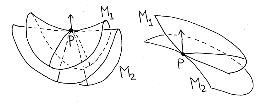
Figure 8. The maximum principle (on the left) and the boundary point maximum principle (on the right). In both cases, the surfaces $M_{1}$ and $M_{2}$ are tangential at $p$ and have the same constant mean curvature with respect to the normal direction $\vec{N}$ at $p$, and $M_{1}$ lies above $M_{2}$ as pictured here. On the right hand side, the boundaries of $M_{1}$ and $M_{2}$ have a common tangent line at $p$. The conclusion in the first case (left hand side) is that $M_{1}$ and $M_{2}$ must coincide in a neighborhood of the point $p$. In the second case (right hand side), $M_{1}$ and $M_{2}$ will coincide in an open set whose closure contains $p$.

Theorem 5.2.

The only embedded compact CMC surfaces in $\mathbb{R}^{3}$ and $\mathbb{H}^{3}$ are the round spheres.

This theorem can be proven using the Alexandrov reflection principle, which is an immediate consequence of the maximum principle (see, for example, [106]). Note that the embeddedness condition in Theorem 5.2 is really necessary, as the CMC Wente tori show (see Chapter 6).

Proof.

The Alexandrov reflection principle works in the following way: Consider the image of a compact embedded CMC surface $M$ in the ambient space $\mathbb{R}^{3}$ or $\mathbb{H}^{3}$. Let $q$ be any fixed point in the ambient space, and let $\vec{v}$ be any unit vector in the tangent space of the ambient space at $q$. Let $\alpha_{\vec{v}}(t)$ be a geodesic in the ambient space such that $\alpha_{\vec{v}}(0)=0$ and $\frac{d}{dt}\alpha_{\vec{v}}(t)|_{t=0}=\vec{v}$. Let $P_{\vec{v},t}$ be the uniquely determined geodesic plane containing $\alpha_{\vec{v}}(t)$ and perpendicular to $\frac{d}{dt}\alpha_{\vec{v}}(t)$. Let

$$L_{\vec{v},t}^{-}=\cup_{s\leq t}P_{\vec{v},s}\;,$$

$$L_{\vec{v},t}^{+}=\cup_{s\geq t}P_{\vec{v},s}\;.$$

Let $t_{0}$ be the smallest value of $t$ such that $P_{t_{0}}\cap M\neq\emptyset$. Then $P_{t_{0}}$ lies to one side of $M$ and contacts $M$ tangentially. For $t>t_{0}$ and sufficiently close to $t_{0}$, the interior of the isometric reflection $R_{t}(M_{\vec{v},t}^{-})$ of the portion $M_{\vec{v},t}^{-}=M\cap L_{\vec{v},t}^{-}$ of $M$ across the plane $P_{t}$ will not make any contact with the portion $M_{\vec{v},t}^{+}=M\cap L_{\vec{v},t}^{+}$ of $M$, and nor will $R_{t}(M_{\vec{v},t}^{-})$ and $M_{\vec{v},t}^{+}$ have any tangential contact along their common boundary. One then continuously increases $t$ until one arrives at the smallest value $t_{1}$ where the reflection $R_{t_{1}}(M_{\vec{v},t_{1}}^{-})$ of $M_{\vec{v},t_{1}}^{-}$ across $P_{t_{1}}$ and $M_{\vec{v},t_{1}}^{+}$ make a tangential contact at some point $p$ in $L_{\vec{v},t_{1}}^{+}$. Let us suppose for the moment that $p$ is in the interior of $L_{\vec{v},t_{1}}^{+}$. Since $t_{1}$ is the smallest such value, $R_{t_{1}}(M_{\vec{v},t_{1}}^{-})$ lies locally to one side of $M_{\vec{v},t_{1}}^{+}$ near $p$. Also, since $M$ is embedded, $R_{t_{1}}(M_{\vec{v},t_{1}}^{-})$ and $M_{\vec{v},t_{1}}^{+}$ have the same orientation with respect to their mean curvature vectors at $p$. Thus $R_{t_{1}}(M_{\vec{v},t_{1}}^{-})$ and $M_{\vec{v},t_{1}}^{+}$ coincide in a neighborhood of $p$. As in the proof of Theorem 5.1, real-analyticity of the frame implies that $R_{t_{1}}(M_{\vec{v},t_{1}}^{-})$ and $M_{\vec{v},t_{1}}^{+}$ are globally identical in $L_{\vec{v},t}^{+}$. Hence $M$ is invariant under isometric reflection across the geodesic plane $P_{\vec{,}t_{1}}$.

When $p$ is not in the interior of $L_{\vec{v},t_{1}}^{+}$, it is in $P_{t_{1}}$. In this case we need a variant of the maximum principle for CMC surfaces, called the boundary point maximum principle for CMC surfaces. This variant will be stated below and gives the same conclusion that $M$ is invariant under isometric reflection across the geodesic plane $P_{\vec{,}t_{1}}$.

We conclude the proof by noting that the direction of $\vec{v}$ was arbitrary, so $M$ has a plane of reflective symmetry in every direction, and this is sufficient to conclude that $M$ is actually a round sphere. ∎

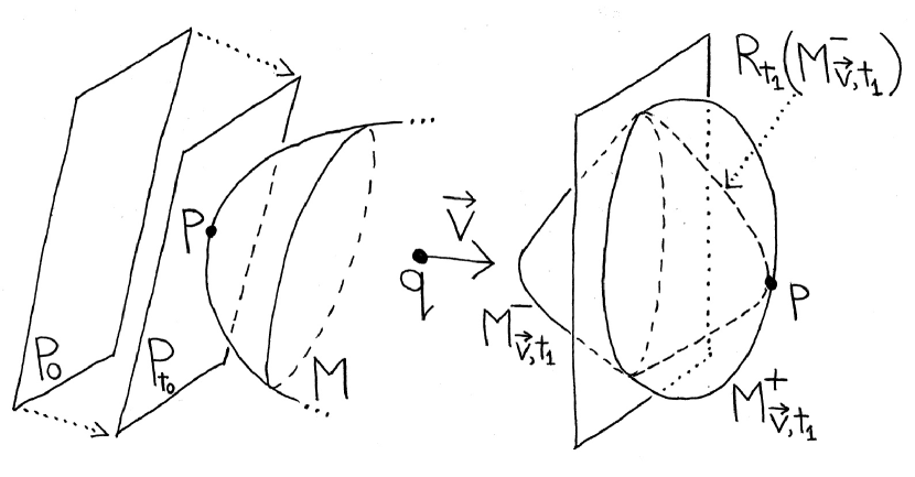
Figure 9. The arguments in the proof of Theorem 5.1 (on the left) and the proof of Theorem 5.2 (on the right).

The maximum principle can also be applied to surfaces with boundary. For example, defining the convex hull of a set to be the smallest convex set that contains it, only can prove the following result similarly to the way Theorem 5.1 was proven:

Theorem 5.3.

The interior of any compact minimal surface in $\mathbb{R}^{3}$ or $\mathbb{H}^{3}$ with boundary must lie in the interior of the convex hull of its boundary.

Many other results have been proven with the maximum principle, among them that any complete connected minimal surface in $\mathbb{R}^{3}$ with two embedded regular ends is a catenoid, proven by Schoen [156]. In addition, Korevaar, Kusner, Meeks, and Solomon ([126], [106]), have proven that any complete nonminimal finite-topology embedded CMC surface with two ends in $\mathbb{R}^{3}$ is a Delaunay surface, and any surface of this type with three ends has a plane of reflective symmetry. Similar results for CMC surfaces in $\mathbb{H}^{3}$ can be found in [107] and [114].

We shall now prepare to give a formal statement and proof of the maximum principle for CMC surfaces. For the sake of simplicity we shall at first assume that the ambient space is $\mathbb{R}^{3}$. However, the arguments here will require only minor changes to become applicable for other ambient spaces as well. For example, the arguments when the ambient space is $\mathbb{H}^{3}$ are very similar, and we will make some remarks about how to prove the $\mathbb{H}^{3}$ case in the final section of this chapter. As the results we have given here are for $\mathbb{R}^{3}$ and $\mathbb{H}^{3}$, we shall restrict ourselves to a discussion of only those two cases.

First we give some preliminaries on the maximum principle for elliptic equations in the next two sections. Much of this material follows [140].

Remark 5.4.

In this chapter, we choose to use $x$ and $x_{j}$ to represent independent variables, and symbols such as $a_{ij},b_{j},f,f_{j},\hat{f},\hat{f}_{j},g,g_{j},h,u$ to represent dependent functions, which is different from the notations in the other chapters of this text. This seems appropriate, however, since this chapter deals with objects of general diminesion, not just $2$-dimensional surfaces, and these notational choices are more standard in the general dimensional case.

5.1. The maximum principle for elliptic equations of a single variable

In order to get some intuition about the maximum principle for elliptic equations, we state and prove various versions of it in the case that there is only one independent variable.

Let us begin with the simplest possible version of the maximum principle. We first consider the case that $u$ is a smooth function

$$u(x):[a,b]\rightarrow\mathbb{R}$$

defined on the closed bounded interval $[a,b]\in\mathbb{R}$, and $L$ is the operator

$$L(u)=u^{\prime\prime}+g(x)u^{\prime}$$

defined on functions $u$ as above, where $g(x)$ is a bounded smooth function on $[a,b]$, and $\prime$ represents the derivative with respect to $x\in[a,b]$. We now state the simplest possible version of the maximum principle:

Lemma 5.5.

(Simplified $1$-dimensional maximum principle) Let $u$, $g$ and $L$ be as above. If $L(u)>0$ on $[a,b]$, then $u$ can attain its maximum value in $[a,b]$ only at the points $x=a$ or $x=b$.

Proof.

Suppose that $u$ attains a local maximum at a point $c\in(a,b)$. Then $u^{\prime}(c)=0$ and $u^{\prime\prime}(c)\leq 0$, so $L(u)(c)\leq 0$, a contradiction. ∎

The above result was particularly easy, because we made the strong assumption that $L>0$. But there is a similar result in the case that we only assume $L\geq 0$, and then the proof is slightly more subtle (and in the application to CMC surfaces we have in mind, we will indeed only know that $L\geq 0$). In this case, $u$ can attain its maximum in the interior of $[a,b]$, but if it does, then $u$ must be a constant function:

Lemma 5.6.

($1$-dimensional maximum principle) Let $u$, $g$ and $L$ be as above. Suppose that $L(u)\geq 0$ on $[a,b]$. If $u\leq M$ on $[a,b]$ for some constant $M\in\mathbb{R}$ and if there exists some $c\in(a,b)$ such that $u(c)=M$, then $u(x)=M$ for all $x\in[a,b]$.

Proof.

Suppose there exists a $c\in(a,b)$ such that $u(c)=M$ and there exists a $d\in(a,b)$ such that $u(d)<M$. Assume for now that $d>c$. Because $g$ is bounded, we may choose a constant $\alpha>\max_{x\in[a,b]}\{|g(x)|\}$, and then we define $y(x)=e^{\alpha(x-c)}-1$. Note that $L(y(x))>0$. It is possible to choose an $\epsilon$ such that $0<\epsilon<\frac{M-u(d)}{y(d)}$, and then we define $w(x)=u+\epsilon y$. $y$ is negative on $(a,c)$, so $w<M$ on $(a,c)$. Note that $w(c)=M$ and $w(d)<M$. So $w$ has an interior maximum in $(a,d)$ and $L(w)>0$. This contradicts Lemma 5.5.

In the case that $d<c$, we may use $y=e^{\alpha(c-x)}-1$ instead of $y=e^{\alpha(x-c)}-1$ and produce a contradiction to Lemma 5.5 in the same way. ∎

Now we consider a more general operator of the form

$$(L+h)(u):=u^{\prime\prime}+gu^{\prime}+hu\;,$$

where $h=h(x)$ is a bounded smooth function on $[a,b]$. Then the condition $L(u)\geq 0$ no longer implies that $u$ attains its maximum at either $x=a$ or $x=b$. Here are two counterexamples:

(1) Let $[a,b]=[0,\pi]$, let $h$ be identically $1$, let $g$ be identically $0$, and let $u=\sin(x)$. Then $(L+h)(u)=u^{\prime\prime}+u=0$, and $u$ has an interior maximum of value $1$ at $x=\frac{\pi}{2}$ and is not maximized at the endpoints $a$ and $b$.

(2) Let $[a,b]=[-1,1]$, let $h$ be identically $-1$, let $g$ be identically $0$, and let $u=-\cosh(x)$. Then $(L+h)(u)=u^{\prime\prime}-u=0$, and $u$ has an interior maximum of value $-1$ at $x=\frac{\pi}{2}$ and is not maximized at the endpoints $a$ and $b$.

These two examples show that nonzero $h$ can cause the operator $L+h$ to not satisfy the maximum principle, regardless of whether $h$ is positive or negative. However, if we assume $h\leq 0$ and $\max_{x\in[a,b]}(u)\geq 0$, then we still have a maximum principle, as we now show:

Lemma 5.7.

(Modified simplified $1$-dimensional maximum principle) If $h\leq 0$ and $(L+h)(u)>0$ on $[a,b]$, then $u$ cannot have a nonnegative maximum in the interior of $[a,b]$.

Proof.

Suppose that $c$ is an interior point of $[a,b]$ where $u$ has a nonnegative local maximum. Then $u^{\prime}(c)=0$, $u^{\prime\prime}(c)\leq 0$, $h(c)u(c)\leq 0$ imply $(L+h)(u)\leq 0$, a contradiction. ∎

Again, if we only have $(L+h)(u)\geq 0$ then this statement above (Lemma 5.7) is not true, but again the only exceptions are when $u$ is constant.

Lemma 5.8.

(Modified $1$-dimensional maximum principle I) If $u$ satisfies $(L+h)(u)\geq 0$ with $h\leq 0$ on $[a,b]$, then if $u$ assumes a nonnegative maximum value $M$ at an interior point $c\in(a,b)$, then $u$ is identically equal to $M$.

Proof.

Assume $M=\max_{x\in[a,b]}\{u\}\geq 0$ on $[a,b]$. Assume there exists an interior point $c$ such that $u(c)=M$. Also, assume there exists an interior point $d$ such that $u(d)<M$. (Suppose for now that $d>c$.) Because $g$ and $h$ are bounded, we can choose an $\alpha\in\mathbb{R}$ so that

$$\alpha^{2}+\alpha g+h(1-e^{-\alpha(x-c)})>0$$

for all $x\in[a,b]$. Then define $y(x)=e^{\alpha(x-c)}-1$, and note that $(L+h)(y)>0$ on $[a,b]$. Set $w=u+\epsilon y$ for some $\epsilon$ such that $0<\epsilon<\frac{M-u(d)}{y(d)}$. As $w<M$ on $(a,c)$, $w(c)=M$, $w(d)<M$, we have that $w$ has an interior maximum point in $(a,d)$. Then, since $(L+h)(w)>0$, we have a contradiction to Lemma 5.7.

Again, if $d<c$, we use $y=e^{\alpha(c-x)}-1$ instead of $y=e^{\alpha(x-c)}-1$. ∎

Now let us consider a different modification of the maximum principle. Here there will be no condition on the sign of $h$ (although $h$ is still assumed to be smooth and bounded). Instead we will assume that $u$ attains a maximum value of precisely $0$ in the interior of the domain. We shall also assume that $u$ is a real analytic function of the independent variable $x$.

Lemma 5.9.

(Modified $1$-dimensional maximum principle II) If a real analytic function $u\leq 0$ on $[a,b]$ satisfies $(L+h)(u)\geq 0$, and if $u(c)=0$ at an interior point $c\in(a,b)$, then $u$ is identically equal to $0$.

Proof.

Suppose that $u$ is not identically zero. Because $u(c)=u^{\prime}(c)=0$, we can expand $u$ at $x=c$ as

$$u=\sum_{j\geq 2}a_{j}(x-c)^{j+\ell}$$

for some nonnegative integer $\ell$ and some $a_{2}\neq 0$. Because $u\leq 0$, we have

(5.1) $$\ell\;\;\text{is an even integer, and }\,a_{2}<0\;.$$

Then $L(u)$ expands as

$$L(u)=(\ell+2)(\ell+1)a_{2}(x-c)^{\ell}(1+\mathcal{O}(x-c))\;.$$

But then (5.1) implies $L(u)<0$ for $x$ close to (but not equal to) $c$. This contradiction proves the lemma. ∎

5.2. The maximum principle for elliptic equations in $n$ variables

Now we consider the $n$-dimensional case, which is entirely analogous to the $1$-dimensional case above. Let $(x_{1},...,x_{n})$ denote points in $\mathbb{R}^{n}$ and let ${\mathcal{D}}$ be an open bounded set in $\mathbb{R}^{n}$ with closure $\overline{{\mathcal{D}}}$. We now consider a smooth function

$$u(x_{1},...,x_{n}):\overline{{\mathcal{D}}}\to\mathbb{R}\;,$$

and we define the operator $L$ by

$$L(u)=\sum_{i,j=1}^{n}a_{ij}(x_{1},...,x_{n})\frac{\partial^{2}}{\partial x_{i}\partial x_{j}}+\sum_{j=1}^{n}b_{j}(x_{1},...,x_{n})\frac{\partial}{\partial x_{j}}$$

defined on functions $u$ as above, where the coefficient functions

$$a_{ij}(x_{1},...,x_{n})\;,\;\;b_{j}(x_{1},...,x_{n})$$

are bounded smooth functions on $\overline{{\mathcal{D}}}$, and $\frac{\partial}{\partial x_{j}}$ represents the partial derivative with respect to $x_{j}$.

Definition 5.10.

$L$ is elliptic in ${\mathcal{D}}$ if $(a_{ij})_{i,j=1}^{n}$ is a positive definite $n\times n$ matrix for all $x\in{\mathcal{D}}$; that is, if at each point in ${\mathcal{D}}$,

$$(y_{1},...,y_{n})(a_{ij})(y_{1},...,y_{n})^{t}\geq\mu(x_{1},...,x_{n})\sum_{j=1}^{n}y_{j}^{2}$$

for some positive function $\mu=\mu(x_{1},...,x_{n})$ on ${\mathcal{D}}$, and any $y_{j}\in\mathbb{R}$.

$L$ is uniformly elliptic on $\overline{{\mathcal{D}}}$ if $\mu(x_{1},...,x_{n})\geq\mu_{0}>0$ for all points in $\overline{{\mathcal{D}}}$, where $\mu_{0}$ is a fixed constant.

This definition is a natural generalization of the Laplacian $\triangle_{1}u(x)=u^{\prime\prime}(x)$ in the definition of $L$ in the $1$-dimensional case, because of the following easily-computed fact: $(a_{ij})$ is positive definite at a point $p\in\overline{{\mathcal{D}}}$ if and only if there exists a linear transformation $\mathcal{A}:(x_{1},...,x_{n})\rightarrow(\tilde{x}_{1},...,\tilde{x}_{n})$ such that the second order part

$$\sum_{i,j=1}^{n}a_{ij}(x_{1},...,x_{n})\frac{\partial^{2}}{\partial x_{i}\partial x_{j}}$$

of $L$ becomes the $n$-dimensional Laplacian

$$\triangle_{n}=\sum_{j=1}^{n}\frac{\partial^{2}}{\partial\tilde{x}_{j}^{2}}$$

at $\mathcal{A}(p)$.

We state the following two results without proof, and refer the reader to [66], [140] for full proofs. However, we note that the ideas behind the proofs are like those in the above proofs for $1$ independent variable. But in the case of $n$ independent variables, there is more bookkeeping involved in the computations, as expected by the greater number of independent variables.

Theorem 5.11.

($n$-dimensional maximum principle) Let $u$ and $L$ be as above. Suppose that $L(u)\geq 0$ and that $L$ is uniformly elliptic on $\overline{{\mathcal{D}}}$. If $u$ attains a maximum value at a point in ${\mathcal{D}}$, then $u$ is a constant function.

Theorem 5.12.

(Modified $n$-dimensional maximum principle I) Let $u$ and $L$ be as above. Suppose that $(L+h)(u)=L(u)+hu\geq 0$ and that $L$ is uniformly elliptic on $\overline{{\mathcal{D}}}$, where $h\leq 0$ is bounded and smooth on $\overline{{\mathcal{D}}}$. If $u$ attains a nonnegative maximum value at a point in ${\mathcal{D}}$, then $u$ is a constant function – in particular, if $h$ is not identically zero, then $u$ must be identically zero.

We also now state (without proof) a higher dimensional version of Lemma 5.9, which could also be used to prove the maximum principle for CMC surfaces that follows. We will not actually use it, as other forms of the maximum principle given here will suffice, but this next theorem is especially useful in proving the maximum principle for CMC surfaces when the ambient space is the $3$-sphere $\mathbb{S}^{3}$. (We do not apply the maximum principle for CMC surfaces in $\mathbb{S}^{3}$ in this text.) Since we would have two independent variables in the application of this theorem to CMC surfaces, we state the result here for only that case. A proof can be found in H. Hopf’s book [79].

Theorem 5.13.

(Modified $2$-dimensional maximum principle II) Consider the operator

$$(L+h)(u):=\partial_{x_{1}}\partial_{x_{1}}u+\partial_{x_{2}}\partial_{x_{2}}u+g_{1}\partial_{x_{1}}u+g_{2}\partial_{x_{2}}u+hu$$

for functions $u:\bar{\mathcal{D}}\to\mathbb{R}$ defined on the closure $\bar{\mathcal{D}}$ of an open bounded domain ${\mathcal{D}}$ of the $2$-dimensional $x_{1}x_{2}$-plane, where $g_{1}$, $g_{2}$ and $h$ are all smooth bounded functions defined on $\bar{\mathcal{D}}$. If a real analytic function $u\leq 0$ on $\bar{\mathcal{D}}$ satisfies $(L+h)(u)\geq 0$, and if $u(p)=0$ at a point $p\in{\mathcal{D}}$, then $u$ is identically equal to $0$.

5.3. Proof of the maximum principle for CMC surfaces in $\mathbb{R}^{3}$

Letting ${\mathcal{D}}$ be an open bounded domain in $\mathbb{R}^{2}$, and letting $f(x_{1},x_{2}):{\mathcal{D}}\to\mathbb{R}$ be a smooth bounded function, we can consider the graph

$$\{\hat{f}(x_{1},x_{2})=(x_{1},x_{2},f(x_{1},x_{2}))\in\mathbb{R}^{3}\,|\,(x_{1},x_{2})\in{\mathcal{D}}\}$$

to be a smooth immersion $\hat{f}$ into $\mathbb{R}^{3}$. Choosing the unit normal to $\hat{f}$ to be the upward-pointing unit normal vector, we saw how to compute the mean curvature $H$ of this surface in Definition 1.3.5 in [59], as half the trace of the shape operator $S$. Because $\hat{f}$ is of the form $(x_{1},x_{2},f(x_{1},x_{2}))$, one can easily compute that ($\delta_{ij}$ is the Kronecker delta function)

(5.2) $$H=\frac{1}{2}\mbox{trace}(S)=\frac{\sum_{i,j=1}^{2}f_{x_{i}x_{j}}(\delta_{ij}(1+(f_{x_{1}})^{2}+(f_{x_{2}})^{2})-f_{x_{i}}f_{x_{j}})}{2(1+(f_{x_{1}})^{2}+(f_{x_{2}})^{2})^{\frac{3}{2}}}\;,$$

where $f_{x_{i}}$ denotes $\partial_{x_{i}}f$ and $f_{x_{i}x_{j}}$ denotes $\partial_{x_{j}}(\partial_{x_{i}}f)$.

Now let $\hat{f}_{1}$ and $\hat{f}_{2}$ be two smooth oriented surfaces with boundary. Suppose that the surface $\hat{f}_{j}$ can be written as a graph over a closed domain $\overline{{\mathcal{D}}}$ for $j=1,2$; that is, that

$$\hat{f}_{j}(x_{1},x_{2})=(x_{1},x_{2},f_{j}(x_{1},x_{2}))$$

for $(x_{1},x_{2})\in\overline{{\mathcal{D}}}$ for some smooth bounded function $f_{j}:\overline{{\mathcal{D}}}\to\mathcal{R}$. Furthermore, suppose that both $\hat{f}_{1}$ and $\hat{f}_{2}$ have the same constant mean curvature $H$ with respect to the orientations given by their upward pointing normals.

Definition 5.14.

We say that $\hat{f}_{1}$ lies above $\hat{f}_{2}$ if $f_{1}\geq f_{2}$ for all points in $\overline{{\mathcal{D}}}$. Then, if

$$p:=(x_{1},x_{2},f_{1}(x_{1},x_{2}))=(x_{1},x_{2},f_{2}(x_{1},x_{2}))$$

(i.e. $f_{1}(x_{1},x_{2})=f_{2}(x_{1},x_{2})$) for some point $(x_{1},x_{2})\in\overline{{\mathcal{D}}}$, and if one of the following two conditions

1. $(x_{1},x_{2})$ is in the interior of $\overline{{\mathcal{D}}}$, or

2. $(x_{1},x_{2})$ is in the boundary of $\overline{{\mathcal{D}}}$, and the tangent planes of $\hat{f}_{1}$ and $\hat{f}_{2}$ coincide at $p$, and furthermore the tangent lines of the boundaries of $\hat{f}_{1}$ and $\hat{f}_{2}$ coincide at $p$

holds, we say that $p$ is a point of common tangency of $\hat{f}_{1}$ and $\hat{f}_{2}$.

We are now ready to state the maximum principle for CMC surfaces in $\mathbb{R}^{3}$:

Proposition 5.15.

(The maximum principle for CMC surfaces in $\mathbb{R}^{3}$.) Let $\hat{f}_{1}$ and $\hat{f}_{2}$ be CMC $H$ graphs with respect to the orientation of upward pointing normals. In particular, $H$ has the same value for both surfaces. Suppose the following:

• $\hat{f}_{1}$ lies above $\hat{f}_{2}$.

• $\hat{f}_{1}$ and $\hat{f}_{2}$ have a point $p$ of common tangency at which the first of the two enumerated items in Definition 5.14 holds.

Then $\hat{f}_{1}$ and $\hat{f}_{2}$ coincide in a neighborhood of $p$.

Proposition 5.16.

(The boundary point maximum principle for CMC surfaces in $\mathbb{R}^{3}$.) Let $\hat{f}_{1}$ and $\hat{f}_{2}$ be CMC $H$ graphs with respect to the orientation of upward pointing normals, just as in Proposition 5.15. In particular, $H$ has the same value for both surfaces. Suppose the following:

• $\hat{f}_{1}$ lies above $\hat{f}_{2}$.

• $\hat{f}_{1}$ and $\hat{f}_{2}$ have a point $p$ of common tangency at which the second of the two enumerated items in Definition 5.14 holds.

Then $\hat{f}_{1}$ and $\hat{f}_{2}$ can be extended to surfaces that coincide in a neighborhood of $p$.

These two results are well known [4], and we include a proof of just the first one here. Proofs can also be found in [156], [51].

Proof.

Applying a rigid motion of $\mathbb{R}^{3}$ if necessary, we may assume $p=(0,0,0)$ is the origin in $\mathbb{R}^{3}$ and that the common tangent plane of the two surfaces is the $x_{1}x_{2}$-plane $\{x_{3}=0\}$. Hence $f_{j}(0,0)=0$ and $(\partial_{x_{1}}f_{j})(0,0)=(\partial_{x_{2}}f_{j})(0,0)=0$, for $j=1,2$.

Equation (5.2) and the fact that both surfaces have the same mean curvature imply that

(5.3) $$\sum_{i,j=1}^{2}\left(w_{ij}\frac{\delta_{ij}(1+|\nabla f_{2}|^{2})-(f_{2})_{x_{i}}(f_{2})_{x_{j}}}{2(1+|\nabla f_{2}|^{2})^{\frac{3}{2}}}+\right.$$

$$(f_{1})_{x_{i}x_{j}}\left(\frac{\delta_{ij}(1+|\nabla f_{2}|^{2})-(f_{2})_{x_{i}}(f_{2})_{x_{j}}}{2(1+|\nabla f_{2}|^{2})^{\frac{3}{2}}}\right.-$$

$$\left.\left.\frac{\delta_{ij}(1+|\nabla f_{1}|^{2})-(f_{1})_{x_{i}}(f_{1})_{x_{j}}}{2(1+|\nabla f_{1}|^{2})^{\frac{3}{2}}}\right)\right)=0\;\;,$$

where $|\nabla f_{j}|^{2}=((f_{j})_{x_{1}})^{2}+((f_{j})_{x_{2}})^{2}$ and

$$w:=f_{2}-f_{1}\leq 0$$

with first derivatives $w_{j}=(f_{2})_{x_{j}}-(f_{1})_{x_{j}}$ and second derivatives $w_{ij}=(f_{2})_{x_{i}x_{j}}-(f_{1})_{x_{i}x_{j}}$. Defining $\beta_{ij}$ by

$$\beta_{ij}(u_{1},u_{2})=\frac{\delta_{ij}(1+u_{1}^{2}+u_{2}^{2})-u_{i}u_{j}}{2(1+u_{1}^{2}+u_{2}^{2})^{\frac{3}{2}}}\;,$$

the intermediate value theorem tells us that

$$\beta_{ij}((f_{2})_{x_{1}},(f_{2})_{x_{2}})-\beta_{ij}((f_{1})_{x_{1}},(f_{1})_{x_{2}})=$$

$$\sum_{k=1}^{2}\left(\left(\frac{\partial}{\partial u_{k}}\beta_{ij}\right)((cf_{2}+(1-c)f_{1})_{x_{1}},(cf_{2}+(1-c)f_{1})_{x_{2}})\right)\cdot(f_{2}-f_{1})_{x_{k}}\;\;,$$

for some $c=c(i,j)\in[0,1]$. Equation (5.3) then has the form

(5.4) $$Lw:=\sum_{i,j=1}^{2}\left(a_{ij}w_{ij}+(f_{1})_{x_{i}x_{j}}\sum_{k=1}^{2}\tilde{b}_{ijk}w_{k}\right)=0\;,$$

where

$$\tilde{b}_{ijk}=\left(\frac{\partial}{\partial u_{k}}\beta_{ij}\right)((cf_{2}+(1-c)f_{1})_{x_{1}},(cf_{2}+(1-c)f_{1})_{x_{2}})\;.$$

Note that $a_{ij},\tilde{b}_{ij},\tilde{b}_{ijk}$ are all bounded functions. Note also that $a_{ij}\approx\frac{\delta_{ij}}{2}$ in a small neighborhood of the origin $(x_{1},x_{2})=(0,0)$, and thus $(a_{ij})$ is a strictly positive definite $2\times 2$ matrix in a small neighborhood of the origin.

Since $w\leq 0$ in a small open neighborhood of $(x_{1},x_{2})=(0,0)$ and has a local maximum $w=0$ at $(0,0)$, it follows from the maximum principle Theorem 5.12 (with $L$ as in (5.4) and $h$ identically equal to zero) that $w$ is identically 0 in a neighborhood of the origin. We conclude that $f_{1}=f_{2}$ near $p$, and thus $\hat{f}_{1}$ and $\hat{f}_{2}$ coincide in a neighborhood of $p$. ∎

5.4. The maximum principle for CMC surfaces in $\mathbb{H}^{3}$

One can give essentially the same proof for the maximum principle for CMC surfaces in other ambient spaces, such as $\mathbb{H}^{3}$. (Some references for the maximum principle in the hyperbolic case are [107], [34], and references therein.) Here we describe how one could prove the maximum principle for CMC surfaces in $\mathbb{H}^{3}$. The arguments go along the same lines as above for $\mathbb{R}^{3}$, but some differences from the Euclidean case are the following:

1. obviously the ambient space no longer has a Euclidean metric (here we will consider the Poincare model for $\mathbb{H}^{3}$, which is conformal to the Euclidean metric), and

2. because the ambient space is not Euclidean, the equation for the mean curvature $H$ of a graph will change.

We now remark on each of these two items.

Regarding the first item: For $\mathbb{H}^{3}$, we can use the Poincare ball model $\mathcal{P}$. This allows us to once again consider the two surfaces locally as graphs over the $x_{1}x_{2}$-plane containing the origin. Since the consideration is only local, the graphs will both lie in the unit ball $\{(x_{1},x_{2},x_{3})\in\mathbb{R}^{3}\,|\,x_{1}^{2}+x_{2}^{2}+x_{3}^{2}<1\}$ that is the Poincare model. The notions of ”point of common tangency” and ”one surface lying above the other” do not change. The only difference is that now the ambient space has the metric

(5.5) $$\lambda^{2}(dx_{1}^{2}+dx_{2}^{2}+dx_{3}^{2})\;,\;\;\;\lambda=\frac{2}{1-x_{1}^{2}-x_{2}^{2}-x_{3}^{2}}\;,$$

like in (3.2).

Regarding the second item: Although this Poincare metric is not Euclidean, it is still conformal to the Euclidean metric, and this conformality will simplify the computation of the mean curvature $H$ for a graph in the Poincare model:

Lemma 5.17.

For a smooth immersion $\hat{f}(x_{1},x_{2})$ in $\mathcal{P}$ written as a graph

$$\hat{f}(x_{1},x_{2})=(x_{1},x_{2},f(x_{1},x_{2}))\in\mathcal{P}$$

with $(x_{1},x_{2})\in{\mathcal{D}}\subset\mathcal{P}\cup\{x_{3}=0\}$, the mean curvature of $\hat{f}$ with respect to its ambient space $\mathcal{P}\approx\mathbb{H}^{3}$ is

(5.6) $$\frac{H}{\lambda}-\frac{\lambda_{N}}{\lambda^{2}}\;,$$

where

1. $H$ is the Euclidean mean curvature as given in Equation (5.2),

2. $\lambda$ is the metric factor of the Poincare metric, as given in (5.5),

3. $\lambda_{N}$ is the derivative of $\lambda$ with respect to the direction $N$, where $N$ is the unit normal vector to $\hat{f}$ with respect to the standard Euclidean space $(\mathbb{R}^{3},dx_{1}^{2}+dx_{2}^{2}+dx_{3}^{2})$.

Remark 5.18.

In fact, the above formula for the mean curvature of a surface in $\mathbb{R}^{3}$ holds for any positive function $\lambda$, when $\mathbb{R}^{3}$ is given the metric $\lambda^{2}(dx_{1}^{2}+dx_{2}^{2}+dx_{3}^{2})$. But because our interest here is specifically in $\mathbb{H}^{3}$, we have fixed $\lambda$ to be the metric factor of the Poincare metric.

Proof.

We will give this proof using the moving frames method.

Note that with respect to the usual Euclidean metric, a surface that is a graph of the form $(x_{1},x_{2},f(x_{1},x_{2}))$ has mean curvature $H$ as in Equation (5.2). For such a graph we define an orthonormal moving frame of vectors $e_{1},e_{2}$ that is an oriented orthonormal frame of vectors for the tangent space of the surface, and then define $e_{3}=N$ to be the unit normal vector to the surface with the upward orientation. We define 1-forms $\omega^{i}$ and $\omega_{i}^{j}$ by

$$\omega^{i}(e_{j})=\delta_{ij}\;\;,\;\;\;\nabla e_{i}=\sum_{j=1}^{3}\omega_{i}^{j}e_{j}\;\;.$$

Note that the $\omega_{i}^{j}$ are skew symmetric, that is, $\omega_{i}^{j}=-\omega_{j}^{i}$. Note also that we have the structure equation

$$d\omega^{i}=\sum_{j=1}^{3}\omega^{j}\wedge\omega_{j}^{i}\;.$$

We can then define the mean curvature as

$$H=\frac{1}{2}\sum_{i=1}^{2}h_{ii}\;,$$

where $h_{ij}=\langle\nabla_{e_{i}}e_{j},e_{3}\rangle=\omega_{j}^{3}(e_{i})$.

If we now consider the same hypersurface, but with the ambient metric $\lambda^{2}(dx_{1}^{2}+dx_{2}^{2}+dx_{3}^{2})$, we can define an orthonormal moving frame in the same way as above. We denote the orthonormal vectors and 1-forms and mean curvature in this case by using the symbols $\hat{e}_{i}$ and $\hat{\omega}^{i}$ and $\hat{\omega}_{i}^{j}$ and $\hat{h}_{ij}$ and $\hat{H}$. Noting that we can take $\hat{e}_{i}=\frac{e_{i}}{\lambda}$ and $\hat{\omega}^{i}=\lambda\omega^{i}$, and using that $\hat{\omega}^{i}\wedge\omega^{i}=0$, we see that (with $\lambda_{j}=e_{j}(\lambda)=d\lambda(e_{j})$ the derivative of $\lambda$ with respect to the direction $e_{j}$)

$$\sum_{j=1}^{3}\hat{\omega}^{j}\wedge\hat{\omega}_{j}^{i} = d\hat{\omega}^{i}=d(\lambda\omega^{i})=d\lambda\wedge\omega^{i}+\lambda d\omega^{i}=\sum_{j=1}^{3}\left(\lambda_{j}\omega^{j}\wedge\omega^{i}+\lambda\omega^{j}\wedge\omega_{j}^{i}\right)$$

$$= \sum_{j=1}^{3}\Bigg{(}\lambda\omega^{j}\wedge\left(\frac{\lambda_{j}}{\lambda}\omega^{i}+\omega_{j}^{i}\right)\Bigg{)}=\sum_{j=1}^{3}\Bigg{(}\hat{\omega}^{j}\wedge\overbrace{\left(\frac{\lambda_{j}}{\lambda}\omega^{i}-\frac{\lambda_{i}}{\lambda}\omega^{j}+\omega_{j}^{i}\right)}^{\mbox{skew symmetric}}\Bigg{)}\;.$$

So we have $\hat{\omega}_{j}^{i}=(\lambda_{j}/\lambda)\omega^{i}-(\lambda_{i}/\lambda)\omega^{j}+\omega_{j}^{i}$. Thus, for $i,j\leq 2$, we have

$$\hat{h}_{ij}=\hat{\omega}_{j}^{3}(\hat{e}_{i})=\left(\frac{\lambda_{j}}{\lambda}\omega^{3}-\frac{\lambda_{3}}{\lambda}\omega^{j}+\omega_{j}^{3}\right)\left(\frac{e_{i}}{\lambda}\right)=\frac{h_{ij}}{\lambda}-\frac{\lambda_{3}}{\lambda^{2}}\delta_{ij}\Longrightarrow\hat{H}=\frac{H}{\lambda}-\frac{\lambda_{3}}{\lambda^{2}}\;,$$

where $\lambda_{3}=N(\lambda)=d\lambda(N)$ is the derivative of $\lambda$ with respect to $N=e_{3}$. ∎

6. Further motivations for studying CMC surfaces

In Chapter 4, we gave Hopf’s theorem showing that any closed CMC surface of genus $0$ in $\mathbb{R}^{3}$ must be a round sphere. Hopf asked if every closed CMC surface must be a round sphere, without any initial assumption about the genus of the surface. In effect, he asked if any closed CMC surface in $\mathbb{R}^{3}$ of any genus must in fact be of genus $0$ and thus be a round sphere.

Evidence to support a positive answer to this question came from the maximum principle for CMC surfaces. This principle gave a technique for showing that any embedded closed CMC surface in $\mathbb{R}^{3}$ must be a round sphere. We gave a proof of this result in Chapter 5. So from this, it follows that a closed CMC surface must be a round sphere if it is either of genus $0$ or is embedded.

So any negative answer to Hopf’s question would need to be an example that is both of positive genus and not embedded. In 1986, H. Wente [170] found exactly such examples, of genus $1$. This discovery of a negative answer to Hopf’s question gave impetus for further research on CMC surfaces. Following Wente’s discovery, U. Abresch [1] in 1987 then published a more explicit representation, using elliptic functions, for closed CMC tori which contain a continuous family of planar principal curves. (Principal curves in a surface are those whose tangent vectors are always a principal curvature direction, and planar curves are those that lie in some plane in $\mathbb{R}^{3}$.) R. Walter [168] (also published in 1987) found an explicit representation for those tori that Abresch considered, using special functions called the Jacobi sn and cn functions. Walter’s representation was developed using the fact that if one family of principal curves are all planar, then the perpendicular principal curves each lie in a sphere. Finally, J. Spruck [160] showed in 1988 that these CMC tori considered by Abresch and Walter are exactly the same surfaces that Wente originally found.

The works mentioned above and the development of the theory of integrable systems since the 1960’s helped lead to the recognition that closed CMC tori could be studied by using techniques from the theory of integrable systems, and that closed CMC tori are special CMC surfaces in the sense that they are of ”finite type”. This is what is shown in the works of U. Pinkall and I. Sterling [135] and A. Bobenko [11] [12] [13], from 1989 to 1991, and in these works all closed CMC tori in $\mathbb{R}^{3}$ were classified.

We mention that also N. Kapouleas, in 1991 and 1995, constructed closed CMC surfaces for every genus $\mathfrak{g}>1$ [87], [88]. But Kapouleas used very different analytic techniques. Further developments in that direction have been presented recently by Kusner, Mazzeo, Pacard, Pollack and Ratzkin as well [109], [118], [119], [120], [121], [141].

The way that the techniques of integrable systems were used in the works of Bobenko was to convert the problem of studying CMC surfaces into the language of $2\times 2$ matrices. The same approach was taken by Dorfmeister, Pedit and Wu when they developed the DPW method in their paper [47] published in 1998. While the language of $2\times 2$ matrices might not seem so natural from the viewpoint of classical differential geometry in $\mathbb{R}^{3}$, it is very natural from the viewpoint of integrable systems, and is certainly convenient for describing the DPW method.

The idea behind the DPW method is that the needed equations and their solutions can be found using holomorphic data and applying a splitting called the Iwasawa decomposition to maps from circles (loops) to $2\times 2$ matrices. This idea dates back at least to I. M. Kričever [108] (1980) and perhaps even earlier, and J. Dorfmeister, F. Pedit and H. Wu formulated it in a way that made the idea apply globally to CMC surfaces [47]. The DPW method was the central topic of [59].

Finally, we note that the integral systems approach to CMC surfaces also helped lead to notions of discrete CMC surfaces. These notions preserve to a large extent the rich mathematical structure associated with smooth CMC surfaces, and this is exactly what we shall focus on for the remainder of this text, from Chapter 8 onward.

But before that, we briefly give an aside on smooth surfaces in indefinite ambient spaces, in Chapter 7.

7. Maximal surfaces in $\mathbb{R}^{2,1}$

In later chapters we consider surfaces in positive definite spaces such as $\mathbb{R}^{3}$, $\mathbb{S}^{3}$ (spherical $3$-space) and $\mathbb{H}^{3}$. However, in this chapter we consider surfaces in a space that is not positive definite. We do this because we have not considered such a type of space yet, and it is informative to see the similarities and differences that occur in the indefinite case. Here we choose maximal surfaces in $\mathbb{R}^{2,1}$ (Minkowski $3$-space), and because the $\mathbb{R}^{4,1}$ Möbius geometric approach of later chapters does not work here, we investigate them in much the same way as we considered minimal surfaces in [59]. It is possible to consider discrete versions of these surfaces [95], and we come back to this in Chapter 10.

We note that this chapter depends on Section 3.4 in [59], and we recommend that the reader look at that before reading this chapter. We also note that this chapter and Chapter 10 are independent of the other chapters here, so could be skipped over without affecting continuity of the text.

Because the maximal surfaces here lie in a space that is not positive definite, they have interesting singularities. The singular points can be cuspidal edges or swallowtails or cuspidal cross caps, generically, and could also be conical singularities, for example, less generically (for related material, see, for example, [62], [100], [146], [147], [148], [149], [151] and [152]). In fact, conical singularities and cuspidal edges and swallowtails exist on the surfaces shown in Figures 10, 11 and 12. We will say more about why this happens below.

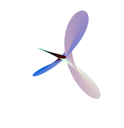
Figure 10. The maximal helicoid (on the left) and Enneper’s maximal surface (on the right). The maximal helicoid cousin is given by the representation of O. Kobayashi with $(g,\eta)=(e^{z},cie^{-z}dz)$, $c\in\mathbb{R}\setminus\{0\}$ on $\Sigma=\mathbb{C}$, like the data for a minimal helicoid in $\mathbb{R}^{3}$. (This maximal helicoid is in fact contained in the image of a minimal helicoid as in Figure 3.4.3 in [59]. See [96] for a proof of this.) Enneper’s maximal surface is given by the representation of O. Kobayashi with $(g,\eta)=(z,cdz)$, $c\in\mathbb{R}\setminus\{0\}$ on $\Sigma=\mathbb{C}$, like the data for an Enneper’s minimal surface in $\mathbb{R}^{3}$. Graphics made by Hitomi Abe and Kouichi Shimose.

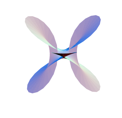
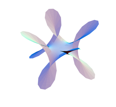
Figure 11. The higher-order versions of Enneper’s maximal surface are given by the representation of O. Kobayashi with $(g,\eta)=(z^{n},cdz)$, $c\in\mathbb{R}\setminus\{0\}$ on $\Sigma=\mathbb{C}$, like the data for higher-order versions of Enneper’s minimal surface in $\mathbb{R}^{3}$. The left-hand side picture is drawn with $n=2$, and the right-hand side picture is drawn with $n=3$. Graphics made by Hitomi Abe and Kouichi Shimose.

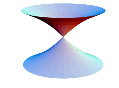
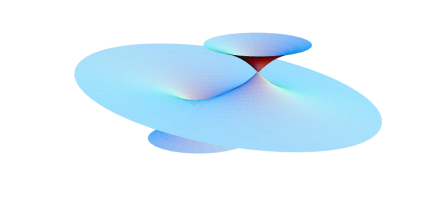
Figure 12. The maximal catenoid (on the left) and the maximal Lopez-Ros surface (on the right). The maximal catenoid is given by the representation of O. Kobayashi with $(g,\eta)=(z,cz^{-2}dz)$, $c\in\mathbb{R}\setminus\{0\}$ on $\Sigma=\mathbb{C}\setminus\{0\}$, like the data for a minimal catenoid in $\mathbb{R}^{3}$ (note that $\Sigma$ is not simply-connnected here, but the surface is a well-defined map from $\Sigma$ to $\mathbb{R}^{2,1}$). The maximal Lopez-Ros surface is given by the representation of O. Kobayashi with $(g,\eta)=(\rho(z^{2}+3)/(z^{2}-1),\rho^{-1}dz)$, $\rho\in(0,\infty)=\mathbb{R}_{+}$ on $\Sigma=\mathbb{C}\setminus\{\pm 1\}$, like the data for a minimal Lopez-Ros surface in $\mathbb{R}^{3}$ (again we have a non-simply-connected domain). Graphics made by Hitomi Abe and Kouichi Shimose

Let $\mathbb{R}^{2,1}=(\{(x_{1},x_{2},x_{0})|x_{j}\in\mathbb{R}\},\langle\cdot,\cdot\rangle_{\mathbb{R}^{2,1}})$ be the $3$-dimensional Minkowski space with the Lorentz metric

$$\langle(x_{1},x_{2},x_{0}),(y_{1},y_{2},y_{0})\rangle_{\mathbb{R}^{2,1}}=x_{1}y_{1}+x_{2}y_{2}-x_{0}y_{0}\;.$$

A surface in $\mathbb{R}^{2,1}$ is called a spacelike surface if the induced metric on the surface is positive definite. In this section we study spacelike surfaces in $\mathbb{R}^{2,1}$ whose mean curvature is identically zero (maximal surfaces). Furthermore, we establish O. Kobayashi’s representation [96] for these surfaces (see also [125]), which is similar to the Weierstrass (Section 3.4 in [59]) and Bryant (Section 5.5 in [59]) and Gálvez, Martínez and Milán (Section 5.6 in [59]) representations, and amongst these three previous representations is most similar to the Weierstrass representation.

Let

$$f:\Sigma\to\mathbb{R}^{2,1}$$

be a conformally immersed spacelike surface, where $\Sigma$ is a simply-connected domain in $\mathbb{C}$ with complex coordinate $z$. (Again, by Theorem 4.5, without loss of generality we may assume $f$ is conformal.) Then

$$\langle f_{z},f_{z}\rangle=\langle f_{\bar{z}},f_{\bar{z}}\rangle=0\;,\;\;\;\langle f_{z},f_{\bar{z}}\rangle=2e^{2\hat{u}}\;,$$

where $\hat{u}:\Sigma\to\mathbb{R}$ is defined this way and $\langle\cdot,\cdot\rangle$ is the complex bilinear extension of $\langle\cdot,\cdot\rangle_{\mathbb{R}^{2,1}}$. Let $N$ be a unit normal vector field of $f$. (Note that $N$ is timelike, that is, $\langle N,N\rangle=-1$, since $f$ is spacelike.) We choose $N$ so that it is future pointing, that is, so that the third coordinate of $N$ is positive. Then

(7.1) $$N:\Sigma\to\mathbb{H}^{2}:=\{\vec{n}=(n_{1},n_{2},n_{0})\in\mathbb{R}^{2,1}\,|\,\langle\vec{n},\vec{n}\rangle=-1\;,\;\;n_{0}>0\}$$

is the Gauss map of $f$.

Note that the target space of the Gauss map is now $\mathbb{H}^{2}$, which is not compact (unlike the case of surfaces in $\mathbb{R}^{3}$, where the target of the Gauss map is the compact $\mathbb{S}^{2}$). Singularities of the maximal surfaces occur when the Gauss map reaches the ideal boundary of $\mathbb{H}^{2}$.

We have the following Gauss-Weingarten equations:

$$f_{zz}=2\hat{u}_{z}f_{z}-QN\;,\quad f_{z\bar{z}}=-2He^{2\hat{u}}N\;,\quad f_{\bar{z}\bar{z}}=2\hat{u}_{\bar{z}}f_{\bar{z}}-\bar{Q}N\;,$$

$$N_{z}=-Hf_{z}-\frac{1}{2}Qe^{-2\hat{u}}f_{\bar{z}}\;,\quad N_{\bar{z}}=-Hf_{\bar{z}}-\frac{1}{2}\bar{Q}e^{-2\hat{u}}f_{z}\;,$$

where $Q:=\langle f_{zz},N\rangle$ is the Hopf differential function and $H=e^{-2\hat{u}}\langle f_{z\bar{z}},N\rangle/2$ is the mean curvature. Also, $(f_{zz})_{\bar{z}}=(f_{z\bar{z}})_{z}$ implies the following Gauss-Codazzi equations:

(7.2) $$4\hat{u}_{z\bar{z}}+Q\bar{Q}e^{-2\hat{u}}-4H^{2}e^{2\hat{u}}=0\;,\quad Q_{\bar{z}}=2H_{z}e^{2\hat{u}}\;.$$

Note that the first equation here has different signs than the corresponding equation for minimal surfaces in $\mathbb{R}^{3}$ (see [59]), although it is otherwise very similar.

Now we identify $\mathbb{R}^{2,1}$ with the Lie algebra

$$\operatorname{su}_{1,1}=\left\{\left.\begin{pmatrix}ia&b\\ \bar{b}&-ia\end{pmatrix}\right|a\in\mathbb{R},\;\;b\in\mathbb{C}\right\}\;,$$

of the Lie group

$$\operatorname{SU}_{1,1}=\left\{\begin{pmatrix}\alpha&\beta\\ \bar{\beta}&\bar{\alpha}\end{pmatrix}\left|\begin{array}[]{c}\alpha,\beta\in\mathbb{C}\\ \alpha\bar{\alpha}-\beta\bar{\beta}=1\end{array}\right.\right\}\;,$$

by identifying $(x_{1},x_{2},x_{0})\in\mathbb{R}^{2,1}$ with the matrix

(7.3) $$x_{1}\sigma_{1}+x_{2}\sigma_{2}+x_{0}i\sigma_{3}=\begin{pmatrix}ix_{0}&x_{1}-ix_{2}\\ x_{1}+ix_{2}&-ix_{0}\end{pmatrix}\in\operatorname{su}_{1,1}\;,$$

where $\sigma_{1}$, $\sigma_{2}$, $\sigma_{3}$ are the Pauli matrices defined in the beginning of Section 3.2 in [59] (but the definition of the Pauli matrices is also apparent from (7.3) here). Note that the metric becomes

$$\langle X,Y\rangle=\frac{1}{2}\text{trace}(XY)$$

when considering $\mathbb{R}^{2,1}$ in this $2\times 2$ matrix model.

The following lemma is immediate:

Lemma 7.1.

If $F\in\operatorname{SU}_{1,1}$, then $\langle X,Y\rangle=\langle FXF^{-1},FYF^{-1}\rangle$ for all $X,Y\in\mathbb{R}^{2,1}$.

We also have the following lemma:

Lemma 7.2.

There exists an $F\in\operatorname{SU}_{1,1}$ (unique up to sign $\pm F$) so that

$$e_{1}:=\frac{f_{u}}{|f_{u}|}=F\sigma_{1}F^{-1}\;,\quad e_{2}:=\frac{f_{v}}{|f_{v}|}=F\sigma_{2}F^{-1}\;,\quad N=Fi\sigma_{3}F^{-1}\;,$$

where $z=u+iv$ for $u,v\in\mathbb{R}$.

Proof.

We first define the Lorentz group $\text{O}_{2,1}$ as the set of $3\times 3$ real valued matrices $A$ which satisfy $A^{t}I_{2,1}A=I_{2,1}$, and the proper Lorentz group as

$$\text{SO}_{2,1}^{+}:=\left\{\!\!\left.A=\begin{pmatrix}a_{11}&a_{12}&a_{10}\\ a_{21}&a_{22}&a_{20}\\ a_{01}&a_{02}&a_{00}\end{pmatrix}\right|\begin{array}[]{c}A\in\text{O}_{2,1}\;,\\ \det A=1\;,\\ a_{00}>0\end{array}\right\}\;,\;\;\text{where}\;\;I_{2,1}:=\begin{pmatrix}1&0&0\\ 0&1&0\\ 0&0&-1\end{pmatrix}\;.$$

Then the correspondence $F\in\operatorname{SU}_{1,1}$ with $(F\sigma_{1}F^{-1},F\sigma_{2}F^{-1},Fi\sigma_{3}F^{-1})$ can be considered as the map $\varphi:\operatorname{SU}_{1,1}\to\text{SO}_{2,1}^{+}$ given by

$$\varphi(F):=\begin{pmatrix}\alpha_{1}^{2}-\alpha_{2}^{2}-\beta_{1}^{2}+\beta_{2}^{2}&2\alpha_{1}\alpha_{2}+2\beta_{1}\beta_{2}&2\alpha_{1}\beta_{2}+2\alpha_{2}\beta_{1}\\ -2\alpha_{1}\alpha_{2}+2\beta_{1}\beta_{2}&\alpha_{1}^{2}-\alpha_{2}^{2}+\beta_{1}^{2}-\beta_{2}^{2}&2\alpha_{1}\beta_{1}-2\alpha_{2}\beta_{2}\\ 2\alpha_{1}\beta_{2}-2\alpha_{2}\beta_{1}&2\alpha_{1}\beta_{1}+2\alpha_{2}\beta_{2}&\alpha_{1}^{2}+\alpha_{2}^{2}+\beta_{1}^{2}+\beta_{2}^{2}\end{pmatrix}$$

via the identification (7.3), where

$$F=\begin{pmatrix}\alpha_{1}+i\alpha_{2}&\beta_{1}+i\beta_{2}\\ \beta_{1}-i\beta_{2}&\alpha_{1}-i\alpha_{2}\end{pmatrix}\;,\;\;\;\alpha_{1},\alpha_{2},\beta_{1},\beta_{2}\in\mathbb{R}\;,\;\;\;\alpha_{1}^{2}+\alpha_{2}^{2}-\beta_{1}^{2}-\beta_{2}^{2}=1\;.$$

One can check that $\varphi$ is a surjective homomorphism, and that $\varphi(F_{1})=\varphi(F_{2})$ if and only if $F_{1}=\pm F_{2}$. This completes the proof. ∎

Therefore, choosing $F$ as in Lemma 7.2, we have $f_{u}=2e^{\hat{u}}F\sigma_{1}F^{-1}$ and $f_{v}=2e^{\hat{u}}F\sigma_{2}F^{-1}$, and so

$$f_{z}=2e^{\hat{u}}F\begin{pmatrix}0&0\\ 1&0\end{pmatrix}F^{-1}\;,\quad f_{\bar{z}}=2e^{\hat{u}}F\begin{pmatrix}0&1\\ 0&0\end{pmatrix}F^{-1}\;.$$

We define $U$ and $V$ by

$$F_{z}=FU\;,\quad F_{\bar{z}}=FV\;.$$

Then, similar to the computation in Section 3.2 of [59], we have

$$U=\frac{1}{2}\begin{pmatrix}-\hat{u}_{z}&-iQe^{-\hat{u}}\\ 2iHe^{\hat{u}}&\hat{u}_{z}\end{pmatrix}\;,\quad V=\frac{1}{2}\begin{pmatrix}\hat{u}_{\bar{z}}&-2iHe^{\hat{u}}\\ i\bar{Q}e^{-\hat{u}}&-\hat{u}_{\bar{z}}\end{pmatrix}\;.$$

Now we consider the case when $f$ is a maximal surface, that is, the mean curvature $H$ is identically zero. (Sufficiently small portions of $H=0$ surfaces in $\mathbb{R}^{2,1}$ actually locally maximize area with respect to arbitrary smooth boundary-fixing variations, rather than minimize area as they would in $\mathbb{R}^{3}$. Hence they are called maximal surfaces rather than minimal surfaces. See [31] and [35], for example.)

Defining functions $a,b:\Sigma\to\mathbb{C}$ so that

$$F=\begin{pmatrix}e^{-\hat{u}/2}\bar{a}&e^{-\hat{u}/2}b\\ e^{-\hat{u}/2}\bar{b}&e^{-\hat{u}/2}a\end{pmatrix}$$

holds, then $a\bar{a}-b\bar{b}=e^{\hat{u}}$, because $F\in\operatorname{SU}_{1,1}$. Since $V=F^{-1}F_{\bar{z}}$, we have

$$\frac{1}{2}\begin{pmatrix}\hat{u}_{\bar{z}}&0\\ i\bar{Q}e^{-\hat{u}}&-\hat{u}_{\bar{z}}\end{pmatrix}=\frac{1}{2}\begin{pmatrix}-\hat{u}_{\bar{z}}+2e^{-\hat{u}}(a\bar{a}_{\bar{z}}-b\bar{b}_{\bar{z}})&2e^{-\hat{u}}(ab_{\bar{z}}-ba_{\bar{z}})\\ 2e^{-\hat{u}}(\bar{a}\bar{b}_{\bar{z}}-\bar{b}\bar{a}_{\bar{z}})&-\hat{u}_{\bar{z}}+2e^{-\hat{u}}(\bar{a}a_{\bar{z}}-\bar{b}b_{\bar{z}})\end{pmatrix}\;.$$

It follows that

$$\begin{pmatrix}\bar{a}&-\bar{b}\\ -b&a\end{pmatrix}\begin{pmatrix}a_{\bar{z}}\\ b_{\bar{z}}\end{pmatrix}=\begin{pmatrix}0\\ 0\end{pmatrix}$$

and so $a_{\bar{z}}=b_{\bar{z}}=0$; that is, $a$ and $b$ are holomorphic.

Note that

$$f_{z}=2e^{\hat{u}}F\begin{pmatrix}0&0\\ 1&0\end{pmatrix}F^{-1}=2\begin{pmatrix}ab&-b^{2}\\ a^{2}&-ab\end{pmatrix}\;,$$

which is holomorphic and is written as

$$f_{z}=(a^{2}-b^{2},-i(a^{2}+b^{2}),-2iab)$$

in the (complexification of the) standard $\mathbb{R}^{2,1}$ coordinates via the identification (7.3). Since $f$ is real-valued, by Remark 3.4.2 in [59], we have

$$\operatorname{Re}\int f_{z}dz=\frac{1}{2}f+(c_{1},c_{2},c_{0})$$

for some constant $(c_{1},c_{2},c_{0})\in\mathbb{R}^{2,1}$. So, up to a translation,

(7.4) $$\begin{array}[]{r@{=}l}f=2\operatorname{Re}\displaystyle\int f_{z}dz&2\operatorname{Re}\displaystyle\int\limits_{\!\!\!}(a^{2}-b^{2},-i(a^{2}+b^{2}),-2iab)dz\\ &\operatorname{Re}\displaystyle\int(1+g^{2},i(1-g^{2}),-2g)\eta\;,\end{array}$$

where $g=-ia/b$ and $\eta=-2b^{2}dz$. This is the Weierstrass-type representation for maximal surfaces as in [96]. We have just shown the following:

Theorem 7.3.

(The representation of O. Kobayashi [96]) Any maximal immersion from a simply-connected domain $\Sigma$ into $\mathbb{R}^{2,1}$ can be given the parametrization (7.4), using a meromorphic function $g:\Sigma\to\mathbb{C}$ and holomorphic 1-form $\eta$ on $\Sigma$.

Also, the metric of the maximal surface is expressed as

$$(1-g\bar{g})^{2}\eta\bar{\eta}=4e^{2\hat{u}}dzd\bar{z}\;.$$

Note that $g\bar{g}>1$, since $a\bar{a}-b\bar{b}>0$. Note also that we have one minus sign on the left side, unlike the plus sign we would have in the case of minimal surfaces in $\mathbb{R}^{3}$, see [59]. This minus sign here allows for singularities, because when $|g|$ approaches $1$ (i.e. the Gauss map approaches the ideal boundary of $\mathbb{H}^{2}$), the metric degenerates and singularities occur.

The normal is

$$N=Fi\sigma_{3}F^{-1}=ie^{-\hat{u}}\begin{pmatrix}a\bar{a}+b\bar{b}&-2\bar{a}b\\ 2a\bar{b}&-(a\bar{a}+b\bar{b})\end{pmatrix}\;,$$

which is written as

$$N = e^{-\hat{u}}\left(i(a\bar{b}-\bar{a}b),a\bar{b}+\bar{a}b,a\bar{a}+b\bar{b}\right)$$

$$= \left(\frac{-g-\bar{g}}{g\bar{g}-1},i\frac{g-\bar{g}}{g\bar{g}-1},\frac{g\bar{g}+1}{g\bar{g}-1}\right)$$

in the standard $\mathbb{R}^{2,1}$ coordinates via the identification (7.3). Thus the function

$$g:\Sigma\to\mathcal{C}:=(\mathbb{C}\cup\{\infty\})\setminus\{z\in\mathbb{C}\;|\;|z|\leq 1\}$$

is the composition of the Gauss map with stereographic projection from $\mathbb{H}^{2}$ (as in (7.1)) to $\mathcal{C}$, and, as noted above, singularities of the surface occur when $|g|$ becomes $1$.

Remark 7.4.

If we assume that the mean curvature $H$ is a non-zero constant, then we have the Sym-Bobenko type formula (see [23])

$$f(z,\bar{z})=\left.\frac{-i}{2H}\left(F\begin{pmatrix}1&0\\ 0&-1\end{pmatrix}F^{-1}+2\lambda(\partial_{\lambda}F)F^{-1}\right)\right|_{\lambda=1}\;.$$

Remark 7.5.

For the purpose of considering spacelike CMC surfaces in $\mathbb{R}^{2,1}$ via the DPW method, we make this remark: Birkhoff splitting for the $\mathbb{R}^{2,1}$ case is the same as in Theorem 4.2.4 in [59], because $\operatorname{SU}_{1,1}$ and $\operatorname{SU}_{2}$ are both real forms of $\operatorname{SL}_{2}\!\mathbb{C}$. ($\operatorname{SU}_{1,1}$ is a noncompact real form and $\operatorname{SU}_{2}$ is the compact real form of $\operatorname{SL}_{2}\!\mathbb{C}$.) However, the product of loop groups $\Lambda\operatorname{SU}_{1,1}\times\Lambda_{+}^{\mathbb{R}}\operatorname{SL}_{2}\!\mathbb{C}$ is now only an open dense subset of $\Lambda\operatorname{SL}_{2}\!\mathbb{C}$, so we do not have a global Iwasawa splitting available for a DPW style construction of spacelike surfaces in $\mathbb{R}^{2,1}$, see [23], [80] and [90]. (When the ambient space is $\mathbb{R}^{3}$, i.e. in the $\operatorname{SU}_{2}$ case, there is a global Iwasawa splitting.)

The non-globalness of the Iwasawa splitting is directly related to singularities on the surfaces, because singularities occur precisely where the Iwasawa splittings associated with the surfaces leave $\Lambda\operatorname{SU}_{1,1}\times\Lambda_{+}^{\mathbb{R}}\operatorname{SL}_{2}\!\mathbb{C}$ (see [23]).

Remark 7.6.

$SU_{1,1}$ is isomorphic as a group to $SL_{2}\mathbb{R}$. For example,

$$\text{SU}_{1,1}\ni\begin{pmatrix}p_{1}+ip_{2}&q_{1}+iq_{2}\\ q_{1}-iq_{2}&p_{1}-ip_{2}\end{pmatrix}\leftrightarrow\begin{pmatrix}p_{1}-q_{1}&p_{2}+q_{2}\\ -p_{2}+q_{2}&p_{1}+q_{1}\end{pmatrix}\in\text{SL}_{2}\mathbb{R}$$

is one such isomorphism, where $p_{j},q_{j}\in\mathbb{R}$ satisfy $p_{1}^{2}+p_{2}^{2}-q_{1}^{2}-q_{2}^{2}=1$. As a result, either $\text{su}_{1,1}$ or $\text{sl}_{2}\mathbb{R}$ can be used to represent $\mathbb{R}^{2,1}$. (Both ways of representing $\mathbb{R}^{2,1}$ can be found in the references [46], [84], [85] and [86].)

8. Linear conserved quantities for smooth CMC surfaces

In the next chapter we introduce an approach to discrete CMC surfaces coming from [27]. But to motivate that discussion, in this chapter we first explain a result of Burstall and Calderbank [26] for the case of smooth CMC surfaces. We begin by describing the $3$-dimensional space forms using the $5$-dimensional Minkowski space $R^{4,1}$.

8.1. Minkowski $5$-space

We give a $2\times 2$ matrix formulation for Minkowski $5$-space. Let $H$ denote the quaternions and $\operatorname{Im}H$ the imaginary quaternions. (We use $H$ to denote both the quaternions and the mean curvature of surfaces, but this should not create any confusion, as it will always be clear from context which meaning $H$ has in each case.)

(8.1) $$\mathbb{R}^{4,1}=\left\{\left.X=\begin{pmatrix}x&x_{\infty}\\ x_{0}&-x\end{pmatrix}\,\right|\,x\in\operatorname{Im}H,x_{0},x_{\infty}\in\mathbb{R}\right\}$$

with Minkowski metric $\langle X,Y\rangle$ such that

(8.2) $$\langle X,Y\rangle\cdot I=-\tfrac{1}{2}(XY+YX)\;,$$

$I$ = identity matrix. This metric has signature $(+,+,+,+,-)$ with respect to the (orthonormal) basis

$$\begin{pmatrix}i&0\\ 0&-i\end{pmatrix}\;,\;\;\begin{pmatrix}j&0\\ 0&-j\end{pmatrix}\;,\;\;\begin{pmatrix}k&0\\ 0&-k\end{pmatrix}\;,\;\;\begin{pmatrix}0&1\\ -1&0\end{pmatrix}\;,\;\;\begin{pmatrix}0&1\\ 1&0\end{pmatrix}\;.$$

If we set $x_{4}=\tfrac{1}{2}(x_{\infty}-x_{0})$, $x_{5}=\tfrac{1}{2}(x_{\infty}+x_{0})$, we can write $X$ as

$$X=x_{1}\begin{pmatrix}i&0\\ 0&-i\end{pmatrix}+x_{2}\begin{pmatrix}j&0\\ 0&-j\end{pmatrix}+x_{3}\begin{pmatrix}k&0\\ 0&-k\end{pmatrix}+x_{4}\begin{pmatrix}0&1\\ -1&0\end{pmatrix}+x_{5}\begin{pmatrix}0&1\\ 1&0\end{pmatrix}\;,$$

where $x=x_{1}i+x_{2}j+x_{3}k$, and then we have the correspondence $X\leftrightarrow(x_{1},x_{2},x_{3},x_{4},x_{5})$ to the more usual way

$$\{\xi=(x_{1},x_{2},x_{3},x_{4},x_{5})\in\mathbb{R}^{5}\,|\,||\xi||=\text{sgn}(\delta)\sqrt{|\delta|},\,\delta=x_{1}^{2}+x_{2}^{2}+x_{3}^{2}+x_{4}^{2}-x_{5}^{2}\}$$

of denoting $\mathbb{R}^{4,1}$. The $4$-dimensional light cone is

$$L^{4}=\{X\in\mathbb{R}^{4,1}\,|\,||X||=0\}\;.$$

We can make the $3$-dimensional space forms as follows: A space form $M$ is

$$M=\{X\in L^{4}\,|\,\langle X,Q\rangle=-1\}$$

for any nonzero $Q\in R^{4,1}$. It will turn out that $M$ has constant sectional curvature $\kappa$, where $Q^{2}=\kappa\cdot I$, so without loss of generality we can obtain any space form by choosing

(8.3) $$Q=\begin{pmatrix}0&1\\ \kappa&0\end{pmatrix}\;,$$

and then, after appropriately scaling $x$, and letting $\operatorname{Im}H\cup\{\infty\}$ denote the one point compactification of $\operatorname{Im}H$, we can write

(8.4) $$M=\left\{\left.X=\frac{2}{1-\kappa x^{2}}\cdot\begin{pmatrix}x&-x^{2}\\ 1&-x\end{pmatrix}\,\right|\,x=x_{1}i+x_{2}j+x_{3}k\in\operatorname{Im}H\cup\{\infty\}\,,\;x^{2}\neq\kappa^{-1}\right\}\,,$$

which is equivalent to $\{(x_{1},x_{2},x_{3})\in\mathbb{R}^{3}\cup\{\infty\}\,|x_{1}^{2}+x_{2}^{2}+x_{3}^{2}\neq-\kappa^{-1}\}$. Note that when $\kappa<0$, $M$ becomes two copies of hyperbolic 3-space with sectional curvature $\kappa$. Also, note the following property:

$$1-\kappa x^{2}\;\;\text{is never zero for points in $M$.}$$

$M$ is called a quadric, because it is determined by a quadratic equation (for the light cone $L^{4}$) and a linear equation (for the hyperplane slicing through $L^{4}$ that produces $M$).

Remark 8.1.

Given any

$$\alpha\begin{pmatrix}x&-x^{2}\\ 1&-x\end{pmatrix}$$

living in the projectivized light cone $PL^{4}$, for any real scalar $\alpha$, we can uniquely choose $\alpha$ so that we get a point in $M$, and so sometimes we can neglect the real scalar $\alpha$, or simply freely choose any $\alpha$ we like.

Remark 8.2.

We have also used the letter $Q$ to denote the Hopf differential function. Wherever we think this might cause confusion, we change the notation for the Hopf differential function to $\hat{Q}$.

The tangent space of $M$ at $X$ is

$$T_{X}M=\left\{\mathcal{T}_{a}=\frac{2}{(1-\kappa x^{2})^{2}}\cdot\begin{pmatrix}a+\kappa xax&-xa-ax\\ \kappa(xa+ax)&-a-\kappa xax\end{pmatrix}\right\}\;,$$

for $a\in\operatorname{Im}H$. When $X=X(t)\in M$ is a smooth function of a real variable $t$, and when $\prime$ denotes differentiation with respect to $t$, we have

$$X^{\prime}=\mathcal{T}_{x^{\prime}}\;.$$

A computation gives

(8.5) $$\langle\mathcal{T}_{a},\mathcal{T}_{b}\rangle=\frac{-4}{(1-\kappa x^{2})^{2}}\text{Re}(ab)\;,$$

$$||\mathcal{T}_{a}||=1\Leftrightarrow|a|=\tfrac{1}{2}|1-\kappa x^{2}|\;.$$

Also,

(8.6) $$X^{\prime\prime}=\mathcal{T}_{\tfrac{2\kappa(xx^{\prime}+x^{\prime}x)}{1-\kappa x^{2}}\cdot x^{\prime}+x^{\prime\prime}}+\frac{4(x^{\prime})^{2}}{(1-\kappa x^{2})^{2}}\cdot\begin{pmatrix}\kappa x&-1\\ \kappa&-\kappa x\end{pmatrix}\;.$$

Note that generally $X^{\prime\prime}$ is not contained in $T_{X}M$.

The following lemma follows from (8.5).

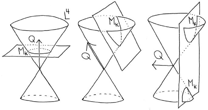
Figure 13. Three choices of $\kappa$ ($\kappa>0$, $\kappa=0$, $\kappa<0$) giving the space forms $\mathbb{S}^{3}$, $\mathbb{R}^{3}$ and (two copies of) $\mathbb{H}^{3}$.

Lemma 8.3.

The $M$ determined by the $Q$ in (8.3) has constant sectional curvature $\kappa$.

We see from (8.5) that the collection of $M$ given by the above choice (8.3) for $Q$, for various $\kappa$, are all conformally equivalent (or Möbius equivalent). In fact, the map $M\ni X\to x\in\text{Im}H\approx\mathbb{R}^{3}$ is stereographic projection when $\kappa\neq 0$. (See Figure 15.)

8.2. Smooth surfaces in space forms

We now consider surfaces in the space forms. Let

$$x=x_{1}(u,v)i+x_{2}(u,v)j+x_{3}(u,v)k\leftrightarrow X=X(u,v)\in M$$

be a surface in $M$. (In this chapter we will use $x$ and $X$ to denote surfaces.) Assume $(u,v)$ is a conformal curvature-line coordinate system (every CMC surface can be parametrized this way, away from umbilic points). We call such coordinates isothermic coordinates.

Note that $x_{1}$, $x_{2}$ and $x_{3}$ can be chosen before the space form $M$ is chosen, and only once $M$ (and hence $\kappa$) is chosen do we know the form of $X$. In particular, the surface can be defined before the space form is chosen.

Remark 8.4.

The phrase ”isothermic coordinates” means simply conformal curvature-line coordinates. However, the phrase ”isothermic surface” will mean for us any surface for which isothermic coordinates exist, even if those isothermic coordinates have not been determined yet.

Notation: Because we will always choose $Q$ as in (8.3), we will indicate this by denoting $M$ as $M_{\kappa}$, with the subscript $\kappa$. We let $n$ denote the unit normal vector for $x$, once $M_{\kappa}$ is chosen. $n_{0}$ denotes the unit normal with respect to Euclidean $3$-space $M_{0}$, where $\kappa=0$. We sometimes write $H_{\kappa}$ for the mean curvature of the surface $x$ with respect to the space form $M_{\kappa}$, to indicate that the mean curvature depends on the choice of space form. $H_{0}$ is the mean curvature in the case of Euclidean $3$-space $M_{0}$.

Lemma 8.5.

The mean curvature $H_{\kappa}$ of $x$ with respect to the space form $M_{\kappa}$ given by $Q$ as in (8.3), with $\triangle x=\partial_{u}\partial_{u}x+\partial_{v}\partial_{v}x$, is

$$H_{\kappa}=\tfrac{-1}{2}|x_{u}|^{-2}\operatorname{Re}\{\triangle x\cdot n\}-\frac{\kappa}{1-\kappa x^{2}}(xn+nx)=$$

$$=\tfrac{-1}{2}(1-\kappa x^{2})|x_{u}|^{-2}\operatorname{Re}\{\triangle x\cdot n_{0}\}-\kappa(xn_{0}+n_{0}x)=$$

$$(1-\kappa x^{2})H_{0}-\kappa(xn_{0}+n_{0}x)\;.$$

Then $H_{\kappa}$ is constant exactly when $\partial_{u}H_{\kappa}=\partial_{v}H_{\kappa}=0$, which is equivalent to

(8.7) $$(\partial_{u}H_{0})\cdot(1-\kappa x^{2})=\kappa\tfrac{k_{2}-k_{1}}{2}\partial_{u}(x^{2})\;,\;\;\;(\partial_{v}H_{0})\cdot(1-\kappa x^{2})=\kappa\tfrac{k_{1}-k_{2}}{2}\partial_{v}(x^{2})\;,$$

where the $k_{j}\in\mathbb{R}$ are the principal curvatures with respect to the Euclidean space form $M_{0}$, i.e. $\partial_{u}n_{0}=-k_{1}\partial_{u}x$ and $\partial_{v}n_{0}=-k_{2}\partial_{v}x$.

Proof.

Letting $x_{1u}$ denote $\tfrac{d}{du}(x_{1})$, and similarly taking other notations, the unit normal vector to the surface is $\mathcal{T}_{n}$, where $n=(1-\kappa x^{2})n_{0}$ and

$$n_{0}=\frac{1}{2}\cdot\frac{(x_{2u}x_{3v}-x_{3u}x_{2v})i+(x_{3u}x_{1v}-x_{1u}x_{3v})j+(x_{1u}x_{2v}-x_{2u}x_{1v})k}{\sqrt{(x_{2u}x_{3v}-x_{3u}x_{2v})^{2}+(x_{3u}x_{1v}-x_{1u}x_{3v})^{2}+(x_{1u}x_{2v}-x_{2u}x_{1v})^{2}}}\;.$$

The first fundamental form $(g_{ij})$ satisfies $\langle\mathcal{T}_{x_{u}},\mathcal{T}_{x_{v}}\rangle=0=g_{12}=g_{21}$, and

$$g_{11}=\langle\mathcal{T}_{x_{u}},\mathcal{T}_{x_{u}}\rangle=\frac{4|x_{u}|^{2}}{(1-\kappa x^{2})^{2}}=\frac{4|x_{v}|^{2}}{(1-\kappa x^{2})^{2}}=\langle\mathcal{T}_{x_{v}},\mathcal{T}_{x_{v}}\rangle=g_{22}\;.$$

Then using (8.6), with the symbol ^′ denoting either $\partial_{u}$ or $\partial_{v}$, we have (where the superscript ”$T$” denotes the part of a vector tangent to $T_{X}M$)

$$b_{11}=\langle X_{uu}^{T},\mathcal{T}_{n}\rangle=\langle X_{uu},\mathcal{T}_{n}\rangle=\frac{-4}{(1-\kappa x^{2})^{2}}\operatorname{Re}\{x_{uu}\cdot n\}+\frac{4\kappa x_{u}^{2}}{(1-\kappa x^{2})^{3}}(xn+nx)\;,$$

$$b_{12}=b_{21}=\langle X_{uv}^{T},\mathcal{T}_{n}\rangle=\langle X_{uv},\mathcal{T}_{n}\rangle=0\;,$$

$$b_{22}=\langle X_{vv}^{T},\mathcal{T}_{n}\rangle=\langle X_{vv},\mathcal{T}_{n}\rangle=\frac{-4}{(1-\kappa x^{2})^{2}}\operatorname{Re}\{x_{vv}\cdot n\}+\frac{4\kappa x_{v}^{2}}{(1-\kappa x^{2})^{3}}(xn+nx)\;.$$

The result follows, using $H_{0}=(k_{1}+k_{2})/2$. ∎

Remark 8.6.

Thomsen proved in the 1920’s that isothermic Willmore surfaces $x$ in the conformal $3$-sphere (i.e. surfaces that are critical with respect to the functional $\int(H^{2}-K)dA$) have a $Q\in\mathbb{R}^{4,1}$ so that $x$ becomes minimal in the space form represented by $Q$. (See the third volume of Blaschke’s texts [10].)

8.3. Spheres

The spheres in any of the space forms $M_{\kappa}$ are the surfaces $x$ such that $|x-C_{0}|$ is constant for some constant $C_{0}\in\text{Im}H$. In the case that $\kappa=0$, if the sphere has radius $r_{0}$, then $r_{0}H_{0}=1$ (in particular, $H_{0}$ is positive with respect to the orientation of $n_{0}$ in the above proof). Thus the sphere can be written as $x=(-1/H_{0})n_{0}+C_{0}$ for some constant $C_{0}$. Then the equation $H_{\kappa}=(1-\kappa x^{2})H_{0}-\kappa(xn_{0}+n_{0}x)$ gives the following formula

(8.8) $$H_{\kappa}=H_{0}-\frac{\kappa}{4H_{0}}-H_{0}\kappa C_{0}^{2}$$

for the relationships between the different mean curvatures for a sphere considered in the different space forms $M_{\kappa}$.

A point

$$\mathcal{S}=\begin{pmatrix}z&z_{\infty}\\ z_{0}&-z\end{pmatrix}$$

in $\mathbb{R}^{4,1}$ with positive norm

$$||\mathcal{S}||=\sqrt{-z^{2}-z_{0}z_{\infty}}>0$$

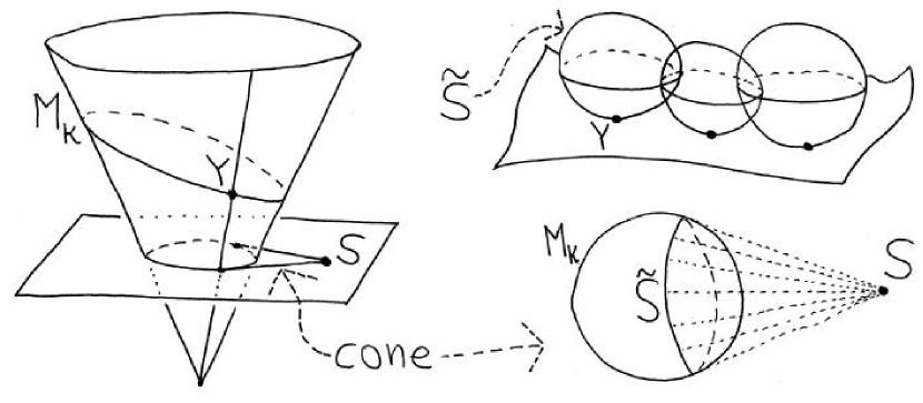
Figure 14. A typical picture of an envelope on the right, and the corresponding picture in the $\mathbb{R}^{4,1}$ model on the left.

determines a sphere $\tilde{\mathcal{S}}$ in the space form $M_{\kappa}$ as follows (see Figure 14): Set

(8.9) $$\tilde{\mathcal{S}}=\{Y\in M_{\kappa}\,|\,\langle Y,\mathcal{S}\rangle=0\}\;.$$

Note that $Y\in\tilde{\mathcal{S}}$ implies $Y$ is perpendicular to $\mathcal{S}-Y$, so $\tilde{\mathcal{S}}$ is the base of the tangent cone from $\mathcal{S}$ to $PL^{4}$, as pictured in Figure 14.

So we have now seen how both points and spheres in the space forms can be described by just points in the single space $\mathbb{R}^{4,1}$, which is a valuable property, from the viewpoint of Möbius geometry. Note that $\tilde{\mathcal{S}}$ is invariant under real scalings of $\mathcal{S}$, and that if $\mathcal{S}$ satisfies $z_{0}=-z_{\infty}$, then $\tilde{\mathcal{S}}$ is a great hypersphere in $M_{1}=\mathbb{S}^{3}$. Also, note that if $||\mathcal{S}||=0$, then $\mathcal{S}$ is a point in $\mathbb{S}^{3}$ and $\tilde{\mathcal{S}}$ is just a real scalar multiple of $\mathcal{S}$, hence $\tilde{\mathcal{S}}$ simply gives back the same point $\mathcal{S}$.

Let $\ell$ be the horizontal line segment from $\mathcal{S}$ to the timelike axis $\{(0,0,0,0,t)\,|\,t\in\mathbb{R}\}$. Then $m=\ell\cap L^{4}$ is a single point, which, when considered as being in the projectivized light cone $PL^{4}$, gives the center of $\tilde{\mathcal{S}}$ in the space form $M_{1}=\mathbb{S}^{3}$.

Lemma 8.7.

Let $\tilde{\mathcal{S}}_{1},\tilde{\mathcal{S}}_{2}$ be two intersecting spheres in $\mathbb{S}^{3}$ produced from $\mathcal{S}_{1},\mathcal{S}_{2}$, respectively, and suppose $||\mathcal{S}_{1}||=||\mathcal{S}_{2}||=1$. Let $\alpha$ be the intersection angle between $\tilde{\mathcal{S}}_{1}$ and $\tilde{\mathcal{S}}_{2}$. Then $\cos\alpha=\pm\langle\mathcal{S}_{1},\mathcal{S}_{2}\rangle$, where the sign on the right hand side depends on the orientations of $\tilde{\mathcal{S}}_{1}$ and $\tilde{\mathcal{S}}_{2}$.

Proof.

As $\kappa=1$, any $p\in\mathbb{S}^{3}=M_{1}$ has $x_{5}$ coordinate equal to $1$. Take $p\in\tilde{\mathcal{S}}_{1}\cap\tilde{\mathcal{S}}_{2}\subset M_{1}$, so $x_{5}(p)=1$. Scale $\mathcal{S}_{1}$ and $\mathcal{S}_{2}$ so that $x_{5}(\mathcal{S}_{1})=x_{5}(\mathcal{S}_{2})=1$. Then $\mathcal{S}_{1}-p$ and $\mathcal{S}_{2}-p$ are normals (in the tangent space of $\mathbb{S}^{3}$) to $\tilde{\mathcal{S}}_{1}$ and $\tilde{\mathcal{S}}_{2}$, respectively, at $p$. So

$$\cos\alpha=\left\langle\frac{\mathcal{S}_{1}-p}{||\mathcal{S}_{1}-p||},\frac{\mathcal{S}_{2}-p}{||\mathcal{S}_{2}-p||}\right\rangle=$$

$$\frac{1}{||\mathcal{S}_{1}-p||}\frac{1}{||\mathcal{S}_{2}-p||}(\langle\mathcal{S}_{1},\mathcal{S}_{2}\rangle-\langle\mathcal{S}_{2},p\rangle-\langle\mathcal{S}_{1},p\rangle+\langle p,p\rangle)=$$

$$\frac{1}{||\mathcal{S}_{1}-p||}\frac{1}{||\mathcal{S}_{2}-p||}(\langle\mathcal{S}_{1},\mathcal{S}_{2}\rangle-0-0+0)=\frac{1}{||\mathcal{S}_{1}||}\frac{1}{||\mathcal{S}_{2}||}\langle\mathcal{S}_{1},\mathcal{S}_{2}\rangle\;.$$

Returning to the scalings for $\mathcal{S}_{1}$ and $\mathcal{S}_{2}$ so that $||\mathcal{S}_{1}||=||\mathcal{S}_{2}||=1$, the lemma is proved. ∎

Remark 8.8.

Lemma 8.7 implies that if $\mathcal{S}$ gives a sphere $\tilde{\mathcal{S}}$ containing $Y\in M_{\kappa}$, then $\{\mathcal{S}+tY\,|\,t\in R\}$ gives a pencil of spheres at $Y$, i.e. the collection of spheres of arbitrary radius through $Y$ and tangent to $\tilde{\mathcal{S}}$.

Lemma 8.9.

Inversion through $\tilde{\mathcal{S}}$ is the map $f:p\to p-2\langle p,\mathcal{S}\rangle\mathcal{S}$, when $||\mathcal{S}||=1$.

Proof.

First note that $p\in L^{4}$ implies $p-2\langle p,\mathcal{S}\rangle\mathcal{S}\in L^{4}$. Now let $C$ be a circle that intersects $\tilde{\mathcal{S}}$ perpendicularly. We wish to show that $p\in C$ implies $f(p)\in C$. Note that $C=\tilde{\mathcal{S}}_{1}\cap\tilde{\mathcal{S}}_{2}$ for some spheres $\tilde{\mathcal{S}}_{1}$ and $\tilde{\mathcal{S}}_{2}$. Then $\tilde{\mathcal{S}}_{1}\perp\tilde{\mathcal{S}}$ and $\tilde{\mathcal{S}}_{2}\perp\tilde{\mathcal{S}}$, and so $\langle\mathcal{S},\mathcal{S}_{1}\rangle=\langle\mathcal{S},\mathcal{S}_{2}\rangle=0$, by the previous lemma. Then $p\in C$ implies $p\in\tilde{\mathcal{S}}_{1}\cap\tilde{\mathcal{S}}_{2}$, which implies $\langle p,\mathcal{S}_{1}\rangle=\langle p,\mathcal{S}_{2}\rangle=0$. Thus $\langle p-2\langle p,\mathcal{S}\rangle\mathcal{S},\mathcal{S}_{1}\rangle=\langle p-2\langle p,\mathcal{S}\rangle\mathcal{S},\mathcal{S}_{2}\rangle=0$, and so $f(p)\in C$. ∎

For further explanation of all this, see [72].

Lemma 8.10.

$\tilde{\mathcal{S}}$ is a sphere with

$$\text{mean curvature}\;\;H_{0}=\frac{|z_{0}|}{2||\mathcal{S}||}\;\;\text{and center}\;\;\frac{z}{z_{0}}$$

in $M_{0}$, and is a sphere with mean curvature $H_{\kappa}$ in $M_{\kappa}$, where $H_{\kappa}$ is as given in Equation (8.8).

Proof.

Take $z=z_{1}i+z_{2}j+z_{3}k$, and consider the case $\kappa=0$. Take

$$Y=2\begin{pmatrix}y&-y^{2}\\ 1&-y\end{pmatrix}\in\tilde{S}\;.$$

Then $YS+SY=0$ implies

$$\sum_{j=1}^{3}(z_{0}y_{j}-z_{j})^{2}=||\mathcal{S}||^{2}\;,$$

and thus $\tilde{\mathcal{S}}$ is a sphere of radius $2||\mathcal{S}||/|z_{0}|$. Hence $H_{0}=|z_{0}|/(2||\mathcal{S}||)$. The final statement of the lemma now follows from Equation (8.8) itself. ∎

8.4. Christoffel transformations

We now define the Christoffel transformation $x^{*}$, which for a CMC surface in $\mathbb{R}^{3}$ gives the parallel CMC surface. Let $x$ be a surface in $\mathbb{R}^{3}$ with mean curvature $H_{0}$ and unit normal $n_{0}$. The Christoffel transformation $x^{*}$ satisfies that

• $x^{*}$ is defined on the same domain as $x$,

• $x^{*}$ has the same conformal structure as $x$,

• $x$ and $x^{*}$ have opposite orientations,

• and $x$ and $x^{*}$ have parallel tangent planes at corresponding points.

One can check that it automatically follows that the principal curvature directions at corresponding points of $x$ and $x^{*}$ will themselves also be parallel.

Remark 8.11.

Let us be careful about what we regard as “opposite orientations” here. With respect to a common orientation for the two parallel tangent planes at a point on $x$ and its corresponding point on $x^{*}$, the two surfaces will have opposite orientations. But if the two surfaces both envelop a common sphere congruence, for which each of the corresponding pairs of points of $x$ and $x^{*}$ tangentially touch the same sphere in the congruence, then $x$ and $x^{*}$ will have the same orientation with respect to the orientation given by a sphere in the sphere congruence. (The surfaces $x$ and $x^{*}$ generally do not envelop a common sphere congruence, but they will when $x$ is CMC and $x^{*}$ is positioned to be the parallel CMC surface of $x$.) The first perspective might be more natural for parallel CMC surfaces, since one moves a constant distance along a normal line to get from one surface to the other, so that normal line provides a common orientation of the two surfaces’ tangent planes, by which the surfaces have oppositie orientation. However, the second perspective might be regarded as more natural for the Darboux transformations that we consider later (since a surface and a Darboux transform of it will always envelop a common sphere congruence).

This description above of the Christoffel transformations turns out to be equivalent to the following definition, and the existence of the integrating factor $\rho$ below is equivalent to the existence of isothermic coordinates. Then, we will see that we can choose $x^{*}$ so that $dx^{*}=x_{u}^{-1}du-x_{v}^{-1}dv$.

Definition 8.12.

A Christoffel transformation $x^{*}$ of an umbilic-free surface $x$ in $\mathbb{R}^{3}$ is a surface that satisfies $dx^{*}=\rho(dn_{0}+H_{0}dx)$ for some nonzero real-valued function $\rho$ on the surface $x$ (here $x^{*}$ is determined only up to translations and homotheties).

Remark 8.13.

The Christoffel transform is also sometimes called the “dual surface”, and “taking the Christoffel transform” can be called “dualizing”.

Remark 8.14.

We did not allow umbilic points on $x$ in the above definition, because they can be troublesome. In particular, the case that $x$ is a round sphere (i.e. is completely umbilic) is very special.

Lemma 8.15.

Away from umbilics of $x$, the Christoffel transform $x^{*}$ exists if and only if $x$ is isothermic.

Proof.

First we prove one direction, by assuming $x$ is isothermic and then showing $x^{*}$ exists.

Take $x$ to be isothermic, and take isothermic coordinates $u,v$ for $x$, so $x_{uv}=Ax_{u}+Bx_{v}$ for some $A,B$. Then

$$d(x_{u}^{-1}du-x_{v}^{-1}dv)=16g_{11}^{-2}(x_{u}x_{uv}x_{u}+x_{v}x_{uv}x_{v})du\wedge dv=0\;.$$

This implies that there exists an $x^{*}$ such that

$$dx^{*}=x_{u}^{-1}du-x_{v}^{-1}dv\;.$$

Also,

$$dn_{0}+H_{0}dx=\tfrac{1}{8}(b_{11}-b_{22})(x_{u}^{-1}du-x_{v}^{-1}dv)\;,$$

implying that $x^{*}$ is a Christoffel transform, since $b_{11}-b_{22}\neq 0$ at non-umbilic points.

Now we prove the other direction, by assuming $x^{*}$ exists and then showing that $x$ has isothermic coordinates.

For any choice of coordinates $u,v$ for $x=x(u,v)$, the Codazzi equations are

$$(b_{11})_{v}-(b_{12})_{u}=\Gamma_{12}^{1}b_{11}+(\Gamma_{12}^{2}-\Gamma_{11}^{1})b_{12}-\Gamma_{11}^{2}b_{22}\;,$$

$$(b_{12})_{v}-(b_{22})_{u}=\Gamma_{22}^{1}b_{11}+(\Gamma_{22}^{2}-\Gamma_{21}^{1})b_{12}-\Gamma_{21}^{2}b_{22}\;.$$

(See, for example, page 97 of [79].) Here the Christoffel symbols are

$$\Gamma_{ij}^{h}=\frac{1}{2}\sum_{k=1}^{2}g^{hk}(\partial_{u_{j}}g_{ik}+\partial_{u_{i}}g_{jk}-\partial_{u_{k}}g_{ij})\;,$$

where $u_{1}=u$ and $u_{2}=v$. Because we are avoiding any umbilic points of $x$, we may assume that $u$ and $v$ are curvature line coordinates for $x$ (see, for example, Appendix B-5 of [165]), and so $g_{12}=b_{12}=0$. It follows that

$$\Gamma_{11}^{1}=\frac{\partial_{u}g_{11}}{2g_{11}}\;,\;\;\Gamma_{22}^{2}=\frac{\partial_{v}g_{22}}{2g_{22}}\;,\;\;\Gamma_{11}^{2}=-\frac{\partial_{v}g_{11}}{2g_{22}}\;,$$

$$\Gamma_{22}^{1}=-\frac{\partial_{u}g_{22}}{2g_{11}}\;,\;\;\Gamma_{12}^{1}=\Gamma_{21}^{1}=\frac{\partial_{v}g_{11}}{2g_{11}}\;,\;\;\Gamma_{12}^{2}=\Gamma_{21}^{2}=\frac{\partial_{u}g_{22}}{2g_{22}}\;.$$

Denoting the principal curvatures by $k_{j}$, the Codazzi equations simplify to

(8.10) $$2(k_{1})_{v}=\frac{\partial_{v}g_{11}}{g_{11}}\cdot(k_{2}-k_{1})\;,\;\;\;2(k_{2})_{u}=\frac{\partial_{u}g_{22}}{g_{22}}\cdot(k_{1}-k_{2})\;.$$

Then existence of $x^{*}$ gives

$$d(\rho dn_{0}+\rho H_{0}dx)=0\;,$$

from which it follows that

$$\begin{pmatrix}0&\frac{b_{11}}{g_{11}}-\frac{b_{22}}{g_{22}}\\ \frac{b_{22}}{g_{22}}-\frac{b_{11}}{g_{11}}&0\end{pmatrix}\begin{pmatrix}\rho_{u}\\ \rho_{v}\end{pmatrix}=\rho\cdot\begin{pmatrix}\left(\frac{b_{11}}{g_{11}}+\frac{b_{22}}{g_{22}}\right)_{v}\\ \left(\frac{b_{11}}{g_{11}}+\frac{b_{22}}{g_{22}}\right)_{u}\end{pmatrix}\;.$$

Then because $\rho_{uv}=\rho_{vu}$ (i.e. it does not matter which order we take mixed derivatives in), we have

$$\left(\frac{(k_{2}+k_{1})_{v}}{k_{1}-k_{2}}\right)_{u}=\left(\frac{(k_{1}+k_{2})_{u}}{k_{2}-k_{1}}\right)_{v}\;,$$

which implies

$$\frac{2(((k_{1})_{v})_{u}+((k_{2})_{u})_{v})}{k_{1}-k_{2}}+2(k_{2}-k_{1})^{-2}\left((k_{1})_{v}(k_{2}-k_{1})_{u}+(k_{2})_{u}(k_{2}-k_{1})_{v}\right)=0\;.$$

Using the Codazzi equations (8.10), we have

$$\left(\log\frac{g_{11}}{g_{22}}\right)_{uv}=0\;.$$

In particular, there exist positive functions $f_{1}(u)$ and $f_{2}(v)$ depending only on $u$ and $v$, respectively, so that

$$(f_{1}(u))^{2}g_{11}=(f_{2}(v))^{2}g_{22}\;.$$

Writing $u=u(\hat{u})$ and $v=v(\hat{v})$ for new curvature line coordinates $\hat{u}$ and $\hat{v}$, we have $\hat{g}_{12}=\hat{b}_{12}=0$ and $\hat{g}_{11}=(u_{\hat{u}})^{2}g_{11}$ and $\hat{g}_{22}=(v_{\hat{v}})^{2}g_{22}$, for the fundamental form entries $\hat{g}_{ij}$ and $\hat{b}_{ij}$ in terms of $\hat{u}$ and $\hat{v}$. We can choose $\hat{u}$ and $\hat{v}$ so that $u_{\hat{u}}=f_{1}(u(\hat{u}))$ and $v_{\hat{v}}=f_{2}(v(\hat{v}))$ hold. Then $\hat{g}_{11}=\hat{g}_{22}$ and so $\hat{u},\hat{v}$ are isothermic coordinates. ∎

Corollary 8.16.

Away from umbilic points, one Christoffel transformation $x^{*}$ of an isothermic surface $x=x(u,v)$ can be taken as a solution of $dx^{*}=x_{u}^{-1}du-x_{v}^{-1}dv$.

Because of $dx^{*}=\rho(dn_{0}+H_{0}dx)$, we have

$$0=d^{2}x^{*}=d\rho\wedge(dn_{0}+H_{0}dx)+\rho\cdot dH_{0}\wedge dx\;,$$

which gives, with respect to isothermic coordinates $(u,v)$, that

(8.11) $$\rho_{u}=-\frac{g_{11}\partial_{u}H_{0}}{g_{11}H_{0}-b_{22}}\cdot\rho\;,\;\;\;\rho_{v}=-\frac{g_{11}\partial_{v}H_{0}}{g_{11}H_{0}-b_{11}}\cdot\rho\;.$$

The existence of $x^{*}$ then automatically implies the compatibility condition $(\rho_{u})_{v}=(\rho_{v})_{u}$, with $\rho_{u}$ and $\rho_{v}$ as just above. This pair of equations tells us that $\rho$ is uniquely determined once its value is chosen at a single point, and thus the solution $\rho$ is unique up to scalar multiplication by a constant factor. Thus the Christoffel transformation in Corollary 8.16 is essentially the unique choice, up to homothety and translation in $\mathbb{R}^{3}$. As a result of this, with essentially no loss of generality, we can now simply take the definition of $x^{*}$ as follows:

Definition 8.17.

The Christoffel transformation of a surface $x$ with isothermic coordinates $(u,v)$ is any $x^{*}$ (defined in $\mathbb{R}^{3}$ up to translation) such that $dx^{*}=x_{u}^{-1}du-x_{v}^{-1}dv$.

Definition 8.17 is slightly more general than Definition 8.12, because it can allow umbilic points in some cases.

Remark 8.18.

The function $\rho$ in Definition 8.12 is generally a constant scalar multiple of the multiplicative inverse of the mean curvature of $x^{*}$, seen as follows: The Christoffel transform of the Christoffel transform $(x^{*})^{*}$, with respect to Definition 8.17, satisfies that

$$d((x^{*})^{*})=(x_{u}^{*})^{-1}du-(x_{v}^{*})^{-1}dv=(x_{u}^{-1})^{-1}du-(-x_{v}^{-1})^{-1}dv=x_{u}du+x_{v}dv=dx\;,$$

so $(x^{*})^{*}$ should be the original surface $x$, up to translation and homothety, with respect to Definition 8.12. Thus, by scaling and translating appropriately, we may assume $(x^{*})^{*}=x$. Also, if the normal of $x$ is $n$, then the normal of $x^{*}$ is $-n$. We have

$$dx=d((x^{*})^{*})=\rho^{*}(dn_{0}^{*}+H_{0}^{*}dx^{*})=\rho^{*}(-dn_{0}+H_{0}^{*}\rho(dn_{0}+H_{0}dx))\;,$$

and so

$$(1-\rho\rho^{*}H_{0}H_{0}^{*})dx=(H_{0}^{*}\rho\rho^{*}-\rho^{*})dn_{0}\;.$$

Since $dx$ and $dn_{0}$ are linearly independent away from umbilic points, it follows that

$$\rho H_{0}^{*}=\rho^{*}H_{0}=1\;.$$

Remark 8.19.

When $H_{0}$ is constant and we have isothermic coordinates, the equations in (8.11) tell us that $\rho$ is constant. Thus if $x^{||}=x+H_{0}^{-1}n_{0}$ is the parallel CMC surface, then $x^{*}$ and $x^{||}$ differ by only a homothety and translation of $\mathbb{R}^{3}$. Thus the Christoffel transformation is essentially the same as the parallel CMC surface to $x$, as expected.

Remark 8.20.

The round cylinder gives one simple example of a Christoffel transform’s orientation reversing property. For the cylinder $x(u,v)=(\cos u,\sin u,v)$ in $\mathbb{R}^{3}$, the normal vector is $n=(-\cos u,-\sin u,0)$, and the Christoffel transform is $x^{*}(u,v)=(-\cos u,-\sin u,v)$ with its normal vector $n^{*}=(\cos u,\sin u,0)$. Thus $n^{*}=-n$. (Note the comments in Remark 8.11.)

Lemma 8.21.

$$dx^{*}=\frac{2}{(k_{1}-k_{2})|x_{u}|^{2}}(dn_{0}+H_{0}dx)\;.$$

Proof.

$$\left(\frac{2}{(k_{1}-k_{2})|x_{u}|^{2}}(dn_{0}+H_{0}dx)-x_{u}^{-1}du+x_{v}^{-1}dv\right)|x_{u}|^{2}=$$

$$=\frac{2}{k_{1}-k_{2}}(-k_{1}x_{u}du-k_{2}x_{v}dv+\tfrac{k_{1}+k_{2}}{2}(x_{u}du+x_{v}dv))+x_{u}du-x_{v}dv=0\;.$$

∎

We have already defined the Hopf differential here and in [59], for a surface in $\mathbb{R}^{3}$, as

$$\hat{Q}dz^{2}\;,\;\;\;\hat{Q}=\langle n_{0},x_{zz}\rangle\;\;\;\;\;(z=u+iv)\;.$$

Corollary 8.22.

If $H_{0}$ is constant for the surface $x=x(u,v)$ in $\mathbb{R}^{3}$ with isothermic coordinates $(u,v)$, then the factor $\hat{Q}$ of the Hopf differential is a real constant.

Proof.

$$\hat{Q}=\tfrac{1}{4}\langle n_{0},x_{uu}-x_{vv}\rangle=(k_{1}-k_{2})|x_{u}|^{2}\;,$$

which is constant by Lemma 8.21 and Remark 8.19. It is clearly also real. ∎

8.5. Conserved quantities and CMC surfaces

In the next definition, we are once again considering general space forms $M$, so the normalization (8.3) is not assumed.

Definition 8.23.

We set

$$\tau=\begin{pmatrix}xdx^{*}&-xdx^{*}x\\ dx^{*}&-dx^{*}x\end{pmatrix}\;.$$

If there exist smooth $Q$ and $Z$ in $\mathbb{R}^{4,1}$ depending on $(u,v)$ such that

(8.12) $$d(Q+\lambda Z)=(Q+\lambda Z)\lambda\tau-\lambda\tau(Q+\lambda Z)$$

holds for all $\lambda\in\mathbb{R}$, then we call $Q+\lambda Z$ a linear conserved quantity of $x$.

We will describe geometric meanings of $Q$, $Z$ and $\tau$ later in this text.

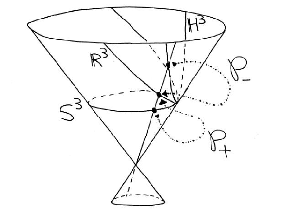
Figure 15. ${\mathcal{P}}_{+}$ and ${\mathcal{P}}_{-}$ are conformal maps from $\mathbb{S}^{3}$ and $\mathbb{H}^{3}$ to $\mathbb{R}^{3}$, showing that $\mathbb{S}^{3}$, $\mathbb{R}^{3}$ and $\mathbb{H}^{3}$ are Möbius equivalent.

Some properties of linear conserved quantities are immediate. For example, $Q$ and $Z^{2}$ are constant, $X\tau=\tau X=0$, $X\perp Z$ and $X\perp dZ$. We now show these properties:

Lemma 8.24.

$Q$ is constant.

Proof.

Set $\lambda=0$ in the conserved quantity equation (8.12). ∎

Lemma 8.25.

$X\tau=\tau X=0$.

Proof.

$$X\tau=\frac{2}{1-\kappa x^{2}}\begin{pmatrix}x\\ 1\end{pmatrix}\begin{pmatrix}1&-x\end{pmatrix}\begin{pmatrix}x\\ 1\end{pmatrix}dx^{*}\begin{pmatrix}1&-x\end{pmatrix}=0\;,$$

since

$$\begin{pmatrix}1&-x\end{pmatrix}\begin{pmatrix}x\\ 1\end{pmatrix}=0\;.$$

Similarly one can show $\tau X=0$. ∎

Lemma 8.26.

If $Q+\lambda Z$ is a linear conserved quantity, then $Z^{2}$ is constant.

Proof.

First note that $d(Z^{2})=Z\cdot dZ+dZ\cdot Z=Z(Q\tau-\tau Q)+(Q\tau-\tau Q)Z=(QZ+ZQ)\tau-\tau(QZ+ZQ)$, since $Z\tau=\tau Z$. Because $QZ+ZQ$ is real, we have $d(Z^{2})=0$. ∎

Lemma 8.27.

$X$ is perpendicular to both $Z$ and $dZ$.

Proof.

$XZ+ZX$ is a real multiple of the identity, and is zero because $\tau(XZ+ZX)=\tau ZX=Z\tau X=Z\cdot 0=0$. Thus, $X\perp Z$. Next, $X\cdot dZ+dZ\cdot X=X(Q\tau-\tau Q)+(Q\tau-\tau Q)X=XQ\tau-\tau QX=(-QX-2\langle X,Q\rangle I)\tau-\tau(-XQ-2\langle X,Q\rangle I)=(2\tau-2\tau)\langle X,Q\rangle=0$. Thus $X\perp dZ$. ∎

Corollary 8.28.

We have $Z^{2}\leq 0$ (i.e. $Z^{2}=\alpha I$ for some $\alpha\leq 0$), and if $Z^{2}=0$, then $Z$ is parallel to $X$.

Proof.

Because $Z$ is perpendicular to $X$, and because $X$ is lightlike, $Z$ is either spacelike, or is a scalar multiple of $X$. So $-Z^{2}\geq 0$, and $-Z^{2}=0$ if and only if $Z$ is parallel to $X$. ∎

Furthermore, when $Z\neq 0$, we will see that $Z^{2}<0$, see Equation (8.15). (That is, $Z^{2}$ cannot be zero.)

Remark 8.29.

Necessary and sufficient conditions for existence of a linear conserved quantity can be stated without ever referring to $\tau$ if we wish, as follows: By definition, a linear conserved quantity exists if and only if there exist $Q=Q(u,v)$ and $Z=Z(u,v)$ in $\mathbb{R}^{4,1}$ such that the following three conditions hold:

1. $Q$ is constant,

2. $dZ=Q\tau-\tau Q$,

3. $Z\tau=\tau Z$.

Note that

$$XdX=\frac{4}{(1-\kappa x^{2})^{2}}\begin{pmatrix}xdx&-xdx\cdot x\\ dx&-dx\cdot x\end{pmatrix}$$

and that $(x^{*})_{u}=x_{u}^{-1}$ and $(x^{*})_{v}=-x_{v}^{-1}$ and $x_{u}^{2}=x_{v}^{2}$, so

$$X\cdot X_{u}=\frac{4x_{u}^{2}}{(1-\kappa x^{2})^{2}}\tau(\partial_{u})\;,\;\;\;X\cdot X_{v}=\frac{-4x_{u}^{2}}{(1-\kappa x^{2})^{2}}\tau(\partial_{v})\;.$$

Then from

$$(XQ+QX)dX-X(dX\cdot Q+Q\cdot dX)=Q\cdot XdX-XdX\cdot Q$$

we have

$$(XQ+QX)X_{u}-X(X_{u}Q+QX_{u})=\frac{4x_{u}^{2}}{(1-\kappa x^{2})^{2}}(Q\cdot\tau(\partial_{u})-\tau(\partial_{u})\cdot Q)$$

and

$$(XQ+QX)X_{v}-X(X_{v}Q+QX_{v})=\frac{-4x_{u}^{2}}{(1-\kappa x^{2})^{2}}(Q\cdot\tau(\partial_{v})-\tau(\partial_{v})\cdot Q)\;.$$

We similarly have that the third condition above becomes

$$ZXX_{u}=XX_{u}Z\;,\;\;\;ZXX_{v}=XX_{v}Z\;.$$

So we can now rewrite the three conditions above, without using $\tau$, as

1. $Q$ is constant,

2. $(XQ+QX)X_{u}-X(X_{u}Q+QX_{u})=\frac{4x_{u}^{2}}{(1-\kappa x^{2})^{2}}Z_{u}$,

3. $(XQ+QX)X_{v}-X(X_{v}Q+QX_{v})=\frac{-4x_{u}^{2}}{(1-\kappa x^{2})^{2}}Z_{v}$,

4. $ZXX_{u}=XX_{u}Z$, $ZXX_{v}=XX_{v}Z$.

Properties like these will be utilized to prove Theorems 8.30 and 8.31 below. The first of these two theorems takes care of the special case that $x$ is a piece of a sphere.

Theorem 8.30.

The surface $x$ in any space form is a part of a sphere if and only if it has a linear conserved quantity that is constant with respect to $\lambda$, that is, of the form $Q+\lambda\cdot 0$.

Proof.

Suppose that $x$ has a conserved quantity $Q$ of order $0$. (Here we are not assuming $Q$ is of the special form in (8.3).) Then $Q+\lambda Z$ will also be a conserved quantity if $Z=\alpha Q$, for some constant $\alpha\in R$. It follows from the above lemmas that $Q$ is constant and $Z$ is either spacelike or parallel to $X$, and $Z$ is perpendicular to $X$. In particular, $Q$ is constant and perpendicular to $X$, and is therefore either spacelike or parallel to $X$. Thus $X$ lies in the sphere given by $\mathcal{S}=Q$, as in (8.9). If $Q$ is lightlike, then $X$ would be a single point, and hence not a surface, so $Q$ must be spacelike (so the curvature $\kappa$ of the space form $M$ given by $Q$ is strictly negative). Thus, in fact, $X$ is part of the virtual boundary sphere at infinity of the spaceform given by $Q$. It follows that $X$ will be part of a finite sphere in other choices for the space form.

Computationally, this can be seen as follows: $Q+\lambda\cdot 0$ is a linear conserved quantity, and the equation for linear conserved quantities implies $Q\tau=\tau Q$. With $Q$ in the form (8.3), it follows that the two equations

$$dx^{*}=-\kappa xdx^{*}x\;,\;\;\;xdx^{*}=-dx^{*}x$$

hold. This in turn implies $dx^{*}=\kappa x^{2}dx^{*}$, and so one of

$$1-\kappa x^{2}=0\;\;\;\text{or}\;\;\;dx^{*}=0$$

must hold. However, because $dx^{*}=x_{u}^{-1}du-x_{v}^{-1}dv$ is never zero, we know that the first of these two equations must hold, and so $x$ is a portion of a sphere (and $\kappa<0$).

Conversely, in the case that $x$ is part of a sphere, then there exists a constant $\mathcal{S}=Q$ that is perpendicular to $X$, and it follows that $Q=Q+\lambda\cdot 0$ itself is a linear conserved quantity, by the four conditions at the end of Remark 8.29. (Note that differentiation of $XQ+QX=0$ gives $dX\cdot Q+Q\cdot dX=0$, because $Q$ is constant.) ∎

Theorem 8.31.

[26] An isothermic immersion $x=x(u,v)$ without umbilic points has constant mean curvature in a space form $M$ (produced by $Q\neq 0$) if and only if there exists (for that $Q$) a linear conserved quantity $Q+\lambda Z$.

Proof.

Assume that $x$ has a linear conserved quantity. We can take $Q$ as in (8.3), and denote the components of $Z$ by

$$Z=\begin{pmatrix}z&z_{\infty}\\ z_{0}&-z\end{pmatrix}\in\mathbb{R}^{4,1}\;.$$

The above lemmas tell us that $XZ+ZX=0$ and $X\perp dZ$, which, respectively, imply

$$xz-x^{2}z_{0}+zx+z_{\infty}=0\;\;\;\text{and}\;\;\;x\,dz-x^{2}dz_{0}+dz\,x+dz_{\infty}=0\;.$$

Differentiating the first of these two equations, and then applying the second one, we have

$$dx\cdot z-(xdx+dx\cdot x)z_{0}+zdx=0\;,$$

which implies $z$ must be of the form

$$z=z_{0}\cdot x+h\cdot n_{0}$$

for some real-valued function $h$. Then

$$x(z_{0}x+hn_{0})-x^{2}z_{0}+(z_{0}x+hn_{0})x+z_{\infty}=hxn_{0}+z_{0}x^{2}+hn_{0}x+z_{\infty}=0\;,$$

so

$$z_{\infty}=-h(xn_{0}+n_{0}x)-z_{0}x^{2}\;.$$

Thus

$$Z=z_{0}\begin{pmatrix}x&-x^{2}\\ 1&-x\end{pmatrix}+h\begin{pmatrix}n_{0}&-n_{0}x-xn_{0}\\ 0&-n_{0}\end{pmatrix}\;.$$

Because $Z^{2}$ is constant,

$$(z_{0}x+hn_{0})^{2}-z_{0}h(xn_{0}+n_{0}x)-z_{0}^{2}x^{2}=-h^{2}/4$$

is constant, and so $h$ is constant, and then also $||Z||$ is constant and nonnegative. A direct computation, using $n_{0}\,dx^{*}+dx^{*}\,n_{0}=0$, now shows that $Z\tau=\tau Z$, so the condition $Z\tau=\tau Z$ coming from Equation (8.12) provides no extra information. The relation $dZ=Q\tau-\tau Q$ from (8.12) gives that

$$dz_{0}=\kappa(x\cdot dx^{*}+dx^{*}\cdot x)\;\text{and}\;dz_{0}\cdot x+z_{0}dx+hdn_{0}=dx^{*}+\kappa xdx^{*}x\;.$$

These two equations give us a pair of (real) equations that are linear with respect to both $h$ and $z_{0}$. Solving simultaneously for $h$ and $z_{0}$ tells us that

(8.13) $$h=\frac{2(1-\kappa x^{2})}{x_{u}^{2}(k_{2}-k_{1})}\;,$$

which we know to be constant, and that

(8.14) $$z_{0}=\tfrac{1}{2}h(k_{2}+k_{1})=h\cdot H_{0}\;.$$

Equations (8.13), (8.14) and $h$ being constant then imply

$$dz_{0}=hdH_{0}=\frac{2(1-\kappa x^{2})}{x_{u}^{2}(k_{2}-k_{1})}dH_{0}\;.$$

Then using that $dz_{0}=\kappa(xdx^{*}+dx^{*}x)$, and that $dx^{*}=x_{u}^{-1}du-x_{v}^{-1}dv$, we find that (8.7) holds, and so $H_{\kappa}$ is constant. One direction of the theorem now follows.

To prove the converse direction, assume that $x$ is a CMC surface with isothermic coordinate $z=u+iv$, then the Hopf differential is a constant multiple of $dz^{2}$ (see Corollary 8.22 here for the case when the space form is $\mathbb{R}^{3}$ and Equations (5.1.1) and (5.2.1) in [59] for other space forms). Thus, looking at the end of the proof of Lemma 8.5, we see that

$$b_{11}-b_{22}=\frac{4x_{u}^{2}(k_{2}-k_{1})}{1-\kappa x^{2}}$$

is constant, and so

$$h=\frac{2(1-\kappa x^{2})}{x_{u}^{2}(k_{2}-k_{1})}$$

is also constant. Take $Q$ as in (8.3), and then take

$$Z=hH_{0}\begin{pmatrix}x&-x^{2}\\ 1&-x\end{pmatrix}+h\begin{pmatrix}n_{0}&-xn_{0}-n_{0}x\\ 0&-n_{0}\end{pmatrix}\;.$$

Then set the candidate for the conserved quantity to be $P=Q+\lambda Z$. Noting that $dx^{*}=x_{u}^{-1}du-x_{v}^{-1}dv$, and $\tau$ is as in Definition 8.23, a computation gives $dP+\lambda\tau P-P\lambda\tau=0$, by Equation (8.7), so $P$ is indeed a linear conserved quantity. ∎

In Theorem 8.31, for given $Q$, when $x$ is constant mean curvature and not totally umbilic, then $Z$ is unique. In fact, in the proof above we saw that $Z$ has the unique form

$$Z=hH_{0}\begin{pmatrix}x+H_{0}^{-1}n_{0}&-x^{2}-H_{0}^{-1}(n_{0}x+xn_{0})\\ 1&-x-H_{0}^{-1}n_{0}\end{pmatrix}\;,$$

where $h$ is the constant as in (8.13). Furthermore, because $1-\kappa x^{2}$ is never zero, $h$ cannot be zero, so the norm of $Z$ satisfies

(8.15) $$||Z||=\tfrac{1}{2}|h|>0\;.$$

In particular, $||Z||\neq 0$.

Also, by Lemma 8.5, the mean curvature satisfies

(8.16) $$H_{\kappa}=-2h^{-1}\langle Z,Q\rangle=-\text{sgn}(h)\frac{1}{||Z||}\langle Z,Q\rangle\;.$$

In particular, if $||Z||=1$, then the mean curvature is $\pm\langle Z,Q\rangle$. Note that any constant scaling of the linear conserved quantity is still a linear conserved quantity, and will change the mean curvature by a constant multiple.

Next, noting that $z_{0}=hH_{0}$, Lemma 8.10 tells us that $Z$ determines a sphere, as in (8.9), in $M_{0}$ with mean curvature

$$\pm\frac{|z_{0}|}{2||Z||}=\pm\frac{|h||H_{0}|}{2\cdot\tfrac{1}{2}|h|}=\pm|H_{0}|\;,$$

so the mean curvature of this sphere is the same as the mean curvature of the surface.

In particular, once we know that the surface and the sphere are tangent, Lemma 8.5 implies that $Z$ determines a sphere congruence for which each sphere has the same mean curvature as the mean curvature at the corresponding point on the surface, regardless of the choice of space form (i.e. the choice of value $\kappa$). Thus $Z$ is the mean curvature sphere congruence (perhaps first defined by Sophie Germain in the first half of the 19’th century), once we know that the spheres determined by $Z$ contain the corresponding points $X$ in the surface and are tangent to the surface, which follow from the next lemma. (In particular, it is not necessary that the surface be of constant mean curvature. We also note one must check that $Z$ and $X$ have common orientation as well, and we leave that to the reader.) In fact, the next lemma reconfirms Lemma 8.27:

Lemma 8.32.

$\langle X,Z\rangle=\langle dX,Z\rangle=0$.

Proof.

$\langle X,Z\rangle\cdot I=-(XZ+ZX)/2=0$ is now immediate. $\langle dX,Z\rangle\cdot I=-(dX\cdot Z+Z\cdot dX)/2=0$ follows from $dx\cdot n_{0}+n_{0}\cdot dx=0$, i.e. $dx$ and $n_{0}$ are perpendicular. ∎

Lemma 8.33.

The mean curvature sphere congruence $Z$ can be characterized as the conformal Gauss map of the surface $X$ (a notion introduced by Robert Bryant), i.e. the unique enveloped sphere congruence that induces the same conformal structure as $X$.

Proof.

That $Z$ is the conformal Gauss map can be seen from the following computation (we do not show uniqueness here):

$$\langle dZ,dZ\rangle=-h^{2}(H_{0}^{2}dx^{2}+H_{0}(dxdn_{0}+dn_{0}dx)+dn_{0}^{2})$$

$$=-h^{2}x_{u}^{2}(\tfrac{1}{4}(k_{1}+k_{2})^{2}(du^{2}+dv^{2})-(k_{1}+k_{2})(k_{1}du^{2}+k_{2}dv^{2})+k_{1}^{2}du^{2}+k_{2}^{2}dv^{2})$$

$$=-\tfrac{1}{4}h^{2}x_{u}^{2}(k_{1}-k_{2})^{2}(du^{2}+dv^{2})\;.$$

∎

Lemma 8.34.

The mean curvature sphere congruence $Z$ can also be characterized as the central sphere congruence (a notion perhaps first defined by Darboux), i.e. the sphere congruence whose spheres exchange the principal curvature spheres via inversion.

Proof.

Let $X=X(u,v)$ be a surface. Take

$$T=T(u,v)=\begin{pmatrix}\ell&\ell_{\infty}\\ \ell_{0}&-\ell\end{pmatrix}\in\mathbb{R}^{4,1}$$

such that $||T||=1$ (i.e. $T$ lies in the de Sitter space $\mathbb{S}^{3,1}$) and

$$\langle T,Q\rangle=\langle T,X\rangle=\langle T,dX\rangle=0\;,$$

with $Q$ as in (8.3). These conditions are equivalent to

• $\ell^{2}+\ell_{0}\ell_{\infty}=-1$,

• $\ell_{\infty}\kappa+\ell_{0}=0$,

• $\ell x+x\ell+\ell_{\infty}-x^{2}\ell_{0}=0$,

• $\ell\cdot dx+dx\cdot\ell-(x\cdot dx+dx\cdot x)\ell_{0}=0$.

Set

$$S_{t}=T+tX=\begin{pmatrix}\ell&\ell_{\infty}\\ \ell_{0}&-\ell\end{pmatrix}+\frac{2t}{1-\kappa x^{2}}\begin{pmatrix}x&-x^{2}\\ 1&-x\end{pmatrix}=:\begin{pmatrix}z&z_{\infty}\\ z_{0}&-z\end{pmatrix}\;.$$

Then $S_{t}$ also lies in $\mathbb{S}^{3,1}$ and is perpendicular to both $X$ and $dX$. By Remark 8.8, the $S_{t}$ represent all of the tangent spheres to $X$. Then, by Equation (8.8) and Lemma 8.10 and a direct computation, the mean curvature of the sphere $S_{t}$ with respect to the space form $M_{\kappa}$ is

$$\frac{|z_{0}|}{2}-\frac{\kappa}{2|z_{0}|}-\kappa\frac{|z_{0}|}{2}\frac{z^{2}}{z_{0}^{2}}=\pm t\;.$$

Then, if $k_{j}$ are the principal curvatures of $X$, $S_{k_{1}}$ and $S_{k_{2}}$ are the principal curvature spheres. By Lemma 8.9, when $Z$ is the central sphere congruence, we should have that

$$S_{k_{2}}=S_{k_{1}}-2\langle S_{k_{1}},Z\rangle\cdot Z\;.$$

However, as we wish to have an inversion that preserves orientation rather than reversing it, we change $S_{k_{2}}$ to $-S_{k_{2}}$. This does not change the sphere itself, as $S_{k_{2}}$ is defined only projectively anyways. Thus the equation becomes

(8.17) $$-S_{k_{2}}=S_{k_{1}}-2\langle S_{k_{1}},Z\rangle\cdot Z\;.$$

Now the image of $S_{k_{1}}$ under inversion and $S_{k_{2}}$ itself will have the same orientation.

We have that $Z=S_{t}$ for some $t$, and so we can now compute from (8.17) that

$$t=\frac{1}{2}(k_{1}+k_{2})\;,$$

i.e. $t$ is the mean curvature. Thus the central sphere congruence is the same as the mean curvature sphere congruence. ∎

Lemma 8.35.

The mean curvature sphere congruence $Z$ can be characterized as the sphere congruence that has second order contact with the surface in orthogonal directions.

Proof.

Principal curvature spheres, second order contact and orthogonality are examples of Möbius invariant notions, because they are invariant under Möbius transformations (such as mapping from one space form to another, as in Figure 15, or inverting through a sphere). Because only Möbius invariant notions appear in this proof, without loss of generality we may assume that the surface $X(u,v)$ lies in $M_{0}=\mathbb{R}^{3}$.

Let $Z$ be the mean curvature sphere at a point $X(u_{0},v_{0})$ of the surface. Then $X(u_{0},v_{0})$ is one point of the sphere $Z$. Let $p$ be a different point in $Z$ and let $S$ be a sphere with center $p$ that intersects $Z$ transversally. We apply inversion $f_{S}$ of $\mathbb{R}^{3}$ through the sphere $S$, so that the point $p$ is mapped to infinity and the sphere $Z$ is thus mapped to a flat plane $f_{S}(Z)$. The image $f_{S}(X(u,v))$ of $X(u,v)$ under inversion will satisfy $H=0$ at the point $f_{S}(X(u_{0},v_{0}))$. Thus the asymptotic directions of $f_{S}(X(u,v))$ at that point are perpendicular to each other, and are also the directions of second order contact with $f_{S}(Z)$. This completes the proof. ∎

We now explain the conserved quantity equation in terms of the Calapso transformation, in order to motivate a definition used in the discrete setting. But first, we consider:

8.6. Inverses of quaternionic matrices and $\text{Mob}(3)$

The Möbius transformations are the maps from $\mathbb{S}^{3}$ to $\mathbb{S}^{3}$ that take $2$-spheres to $2$-spheres. We now describe them algebraically, using quaternionic matrices.

First we need the following lemma, which follows from the properties $\text{Re}(x)=\text{Re}(\bar{x})$ and $\text{Re}(xy)=\text{Re}(yx)$, where $x$ and $y$ are quaternions:

Lemma 8.36.

For $a,b,c,d\in H$, we have

$$\text{Re}(abcd)=\text{Re}(\bar{d}\bar{c}\bar{b}\bar{a})=\text{Re}(\bar{b}\bar{a}\bar{d}\bar{c})=\text{Re}(bcda)\;.$$

For later use, we also give the following lemma:

Lemma 8.37.

Suppose that $p,q,r,s\in\text{Im}H$ and $(p-q)(q-r)(r-s)(s-p)\in\mathbb{R}$. Then

$$(p-q)(q-r)(r-s)(s-p)=(s-p)(r-s)(q-r)(p-q)=$$

$$(q-r)(p-q)(s-p)(r-s)=(q-r)(r-s)(s-p)(p-q)\;.$$

Take a quaternionic $2\times 2$ matrix

$$T=\begin{pmatrix}a&b\\ c&d\end{pmatrix}\;.$$

Then the Study determinant $[T]$ of $T$ is the determinant of $T\cdot\bar{T}^{t}$, i.e.

$$[T]=(a\bar{a}+b\bar{b})(c\bar{c}+d\bar{d})-(a\bar{c}+b\bar{d})(c\bar{a}+d\bar{b})=|a|^{2}|d|^{2}+|b|^{2}|c|^{2}-b\bar{d}c\bar{a}-a\bar{c}d\bar{b}\;,$$

and this is clearly a real number. (Note that $\det T$ itself is not a well defined notion, as quaternions do not commute.) When $[T]\neq 0$, we can define the inverse of $T$ as

$$T^{-1}=\frac{1}{[T]}\begin{pmatrix}|d|^{2}\bar{a}-\bar{c}d\bar{b}&|b|^{2}\bar{c}-\bar{a}b\bar{d}\\ |c|^{2}\bar{b}-\bar{d}c\bar{a}&|a|^{2}\bar{d}-\bar{b}a\bar{c}\end{pmatrix}\;.$$

One can check that $T^{-1}T=TT^{-1}=I$, by using Lemma 8.36.

In general, for $A\in\mathbb{R}^{4,1}$, $TAT^{-1}$ might not lie in $\mathbb{R}^{4,1}$, i.e. we might not have

$$TAT^{-1}=\begin{pmatrix}x&x_{\infty}\\ x_{0}&-x\end{pmatrix}\;,\;\;\;x_{0},x_{\infty}\in\mathbb{R}\;,\;\;\;x\in\operatorname{Im}H\;.$$

To avoid such a problem, we define a set, call in $G$, as all $2\times 2$ quaternionic matrices $T$ so that

(8.18) $$\bar{b}d+\bar{d}b=\bar{a}c+\bar{c}a=0\;,\;\;\;\bar{a}d+\bar{c}b\in\mathbb{R}$$

and

(8.19) $$\bar{a}d+\bar{c}b\neq 0\;.$$

Then (8.19) implies

$$[T]=(\bar{a}d+\bar{c}b)\overline{(\bar{a}d+\bar{c}b)}>0$$

and $T\in G$ will have an inverse. By Equation (8.18) and the fact that $\bar{a}d+\bar{c}b\neq 0$, we find, when

$$A=\alpha\begin{pmatrix}x&x_{\infty}\\ x_{0}&-x\end{pmatrix}\;,\;\;\;x\in\operatorname{Im}H\;,\;\;\;\alpha,x_{0},x_{\infty}\in\mathbb{R}\;,$$

that

$$[T]\cdot TAT^{-1}=$$

$$=\alpha(\bar{a}d+\bar{c}b)\cdot\left[\begin{pmatrix}ax\bar{d}-bx\bar{c}&ax\bar{b}-bx\bar{a}\\ cx\bar{d}-dx\bar{c}&cx\bar{b}-dx\bar{a}\end{pmatrix}+x_{0}\begin{pmatrix}b\bar{d}&b\bar{b}\\ d\bar{d}&d\bar{b}\end{pmatrix}+x_{\infty}\begin{pmatrix}a\bar{c}&a\bar{a}\\ c\bar{c}&c\bar{a}\end{pmatrix}\right]\in\mathbb{R}^{4,1}\;.$$

In particular, we have $TAT^{-1}\in\mathbb{R}^{4,1}$. If, furthermore, $x_{0}=1$ and $x_{\infty}=-x^{2}$, i.e. $A\in L^{4}$, then we also have that $TAT^{-1}$ is in $L^{4}$, and this follows from the property

$$[T_{1}T_{2}]=[T_{1}]\cdot[T_{2}]\;,\;\;\;T_{j}\in G\;,$$

for Study determinants.

The set $G$ is a group. For example, if $T_{1}$ and $T_{2}$ are in $G$, then so is $T_{1}T_{2}$.

When $A$ is an element of $L^{4}$, and consequently $TAT^{-1}$ is as well, the ratio of the upper left and lower left entries of $TAT^{-1}$ will be $(ax+b)(cx+d)^{-1}\in\operatorname{Im}H$. In this way, the $T\in G$ are related to Möbius transformations by

(8.20) $$\left(T=\begin{pmatrix}a&b\\ c&d\end{pmatrix}\right)*x=(ax+b)(cx+d)^{-1}\;.$$

Thus, when $A\in L^{4}$, then $TAT^{-1}$ is essentially the same map as (8.20).

Note that, in Equation (8.20), we place the inverse $(cx+d)^{-1}$ to the right side of $(ax+b)$. (Because quaternions do not commute, placing this term on the other side would not give the same result.)

Remark 8.38.

In fact, Equation (8.20) gives both orientation preserving and orientation reversing Möbius transformations. For example, $\text{Im}H\ni x\to(0\cdot x+1)(1\cdot x+0)^{-1}=x^{-1}=-x/|x|^{2}\in\text{Im}H$ is orientation preserving, while $\text{Im}H\ni x\to(0\cdot x-1)(1\cdot x+0)^{-1}=-x^{-1}=x/|x|^{2}\in\text{Im}H$ is orientation reversing.

Furthermore, because

$$\langle TAT^{-1},TBT^{-1}\rangle=\langle A,B\rangle$$

for any $A,B\in\mathbb{R}^{4,1}$, the map $A\to TAT^{-1}$ is an isometry of $\mathbb{R}^{4,1}$.

When $\kappa\neq 0$, i.e. when $Q$ as in (8.3) is not null, $M_{\kappa}$ has a particular Möbius transformation called the antipodal map, which we now describe: A point $X$ in $M_{\kappa}$ can be decomposed as

$$X=\frac{2}{1-\kappa x^{2}}\begin{pmatrix}x&-x^{2}\\ 1&-x\end{pmatrix}=\mathcal{A}+\kappa^{-1}Q\;,$$

where

$$\mathcal{A}=\frac{2}{1-\kappa x^{2}}\begin{pmatrix}x&-x^{2}\\ 1&-x\end{pmatrix}-\kappa^{-1}Q$$

is perpendicular to $Q$. The antipodal map is

$$\mathcal{A}+\kappa^{-1}Q\to-\mathcal{A}+\kappa^{-1}Q\;,$$

that is, we are moving the point $X$ to another point in $M_{\kappa}$ that is on the opposite side of $Q$. Since

$$-\mathcal{A}+\kappa^{-1}Q=\frac{2}{1-\kappa(\kappa^{-1}x^{-1})^{2}}\begin{pmatrix}\kappa^{-1}x^{-1}&-(\kappa^{-1}x^{-1})^{2}\\ 1&-\kappa^{-1}x^{-1}\end{pmatrix}\;,$$

the antipodal map is the Möbius transformation $x\to\kappa^{-1}x^{-1}$.

Remark 8.39.

Möbius transformations of the ambient space preserve the conformal structure of the space, so will preserve the conformal structure of any surface inside the space as well. Furthermore, Möbius transformations will preserve contact order of any spheres tangent to the surface, and so will preserve the principal curvature spheres. It follows that if $x(u,v)$ is an isothermic parametrization of a surface, it will remain an isothermic parametrization even after a Möbius transformation is applied.

Definition 8.40.

Mob(3) is the collection of Möbius transformations $L^{4}\ni A\to TAT^{-1}\in L^{4}$, for $T\in G$.

Remark 8.41.

Mob(3) is a 10-dimensional object, while $G$ is an 11-dimensional object.

Now we make some comments about Möbius transformations in general dimension. Möbius transformations of the $n$-dimensional sphere $\mathbb{S}^{n}$, $n\geq 2$, are maps that take points in $\mathbb{S}^{n}$ to points in $\mathbb{S}^{n}$ and also hyperspheres in $\mathbb{S}^{n}$ to hyperspheres in $\mathbb{S}^{n}$. We denote the collection of Möbius transformations of $\mathbb{S}^{n}$ by Mob($n$). We have the following facts:

Fact: Let Conf_g($n$) denote the global conformal transformations of all of $\mathbb{S}^{n}$, and let Conf_ℓ($n$) denote the local conformal transformations of local domains of $\mathbb{S}^{n}$. Then

$$\text{Mob}(2)=\text{Conf}_{g}(2)\subset Conf_{\ell}(2)\;,\;\;\;\text{Conf}_{g}(2)\neq Conf_{\ell}(2)$$

and

$$\text{Mob}(n)=\text{Conf}_{g}(n)=Conf_{\ell}(n)$$

for $n\geq 3$.

The reason the case $n=2$ is different is that holomorphic functions from $\mathbb{C}$ to $\mathbb{C}$ can be pulled back by the inverse of stereographic projection to maps from $\mathbb{S}^{2}$ to $\mathbb{S}^{2}$, and those maps are generally in $\text{Conf}_{\ell}(2)$ but not in $\text{Conf}_{g}(2)$. This occurs only in the case $n=2$.

Fact: Let $f\in\text{Conf}_{\ell}(n)$ with $n\geq 3$. Let $M\subset\mathbb{S}^{n}$ be a smooth hypersurface. Then $p\in M$ is an umbilic point if and only if $f(p)\subset f(M)$ is an umbilic point as well.

Remark 8.42.

$O(n+1,1)$ is the set of orthogonal transformations of $\mathbb{R}^{n+1,1}$, and these transformations preserve the set of lines in the light cone, as well as the set of spacelike lines, and

$$\frac{O(n+1,1)}{\{\pm I\}}\subset\text{Mob}(n)\;,$$

and in fact, these two sets are equal.

Remark 8.43.

Projective transformations are maps from projective space $P\mathbb{R}^{n+2}$ to $P\mathbb{R}^{n+2}$, i.e. from lines in $\mathbb{R}^{n+2}$ through the origin to lines in $\mathbb{R}^{n+2}$ through the origin, so that ”lines of lines”, which can generically be represented by lines in $\{x_{n+2}=1\}$ ($x_{n+2}$ is the final Cartesian coordinate of points $(x_{1},...,x_{n+2})\in\mathbb{R}^{n+2}$), get mapped to ”lines of lines”. The fundamental theorem of projective geometry, a nontrivial result, is this: Any projective transformation comes from a linear map of $\mathbb{R}^{n+2}$. Then, regarding $\mathbb{R}^{n+2}$ as $\mathbb{R}^{n+1,1}$ (i.e. changing the Euclidean metric to the Minkowski metric), those projective transformations that preserve the light cone are equivalent to Mob($n$).

8.7. Calapso transformations

In the following definition, the surface $x$ lies in some space form $M$, but since we are dealing with a Möbius geometric notion, the choice of space form will not matter.

Definition 8.44.

Let $x=x(u,v)$, with associated $X=X(u,v)\in M$, be an immersed surface with isothermic coordinates $u,v$. A Calapso transformation $T\in\text{Mob}(3)$ is a solution of

$$T^{-1}dT=\lambda\tau\;.$$

Then the transform $\text{Im}H\ni x\to T*x\in\text{Im}H$, where $*$ denotes the Möbius transformation as in (8.20), or equivalently $L^{4}\ni X\to TXT^{-1}\in L^{4}$, is a Calapso transform. (We can also call it a $T$-transform or conformal deformation.)

Remark 8.45.

If we write $T$ as

$$T=\begin{pmatrix}a&b\\ c&d\end{pmatrix}\;,$$

then the equation $dT=T\cdot\lambda\tau$ gives

$$(\bar{b}d+\bar{d}b)_{u}=(\bar{b}d+\bar{d}b)_{v}=(\bar{a}c+\bar{c}a)_{u}=(\bar{a}c+\bar{c}a)_{v}=(\bar{a}d+\bar{c}b)_{u}=(\bar{a}d+\bar{c}b)_{v}=0\;,$$

and so if the initial condition for the solution $T$ lies in $\text{Mob}(3)$, then $T$ will always lie in $\text{Mob}(3)$.

Remark 8.46.

Although we will not be particularly precise about this, we will generally use the word ”transformation” when the object under consideration is a procedure toward a separate goal, and the word ”transform” for the desired goal.

The Calapso transformation is classical, and was studied by Calapso, Bianchi and Cartan. It preserves the conformal structure and is thus of interest in Möbius geometry. In the case that the starting surface is CMC, it is the same as the Lawson correspondence (see Remark 11.27), which is an important transformation in the differential geometry of CMC surfaces.

Lemma 8.47.

If $x$ is isothermic, then Calapso transformations exist.

Proof.

The compatibility condition for the system

$$T^{-1}T_{u}=\lambda U\;,\;\;\;U=\begin{pmatrix}x\\ 1\end{pmatrix}x_{u}^{-1}\begin{pmatrix}1&-x\end{pmatrix}\;,$$

$$T^{-1}T_{v}=\lambda V\;,\;\;\;V=-\begin{pmatrix}x\\ 1\end{pmatrix}x_{v}^{-1}\begin{pmatrix}1&-x\end{pmatrix}$$

to have a solution $T$ is

$$\lambda(UV-VU)+V_{u}-U_{v}=0\;,$$

and this condition holds precisely because of the conditions for isothermicity, that is

(8.21) $$x_{u}^{2}=x_{v}^{2}\;,\;\;x_{u}x_{v}+x_{v}x_{u}=0\;,\;\;x_{uv}=Ax_{u}+Bx_{v}$$

for some functions $A,B$. By Remark 8.45, we have that $T$ always lies in $\text{Mob}(3)$ if it does at any one point, i.e. if the initial condition for $T$ is chosen to be in $\text{Mob}(3)$, completing the proof. ∎

If the surface $x$ has a linear conserved quantity $P=Q+\lambda Z$, then

$$dP+\lambda\tau P-P\lambda\tau=0$$

holds, i.e. $dP+T^{-1}dT\cdot P-P\cdot T^{-1}dT=0$, which is equivalent to

(8.22) $$d(TPT^{-1})=0\;,$$

that is to say, $TPT^{-1}$ is constant. It is $TPT^{-1}$ being constant that we will use to define discrete CMC surfaces, just as it defines smooth CMC surfaces, by Theorem 8.31.

In Möbius geometry (in the space $\mathbb{R}^{4,1}$), isothermic surfaces are deformable (Calapso transformations), and this deformation preserves second order invariants in Möbius geometry, such as conformal class, and conformal class of the trace-free second fundamental form. (Note that for surfaces in Euclidean geometry, a nontrivial deformation will never preserve the second order invariants, i.e. the first and second fundamental forms, of Euclidean geometry.)

Remark 8.48.

Because

$$\lambda\tau=T^{-1}dT\;,$$

$\lambda\tau$ can be thought of as the logarithmic derivative of the Calapso transformation.

8.8. Darboux transformations

For smooth surfaces, a Darboux transform is one such that

• there exists a sphere congruence enveloped by the original surface and the transform,

• the correspondence, given by the sphere congruence, from the original surface to the other enveloping surface (i.e. the transform), preserves curvature lines,

• this correspondence preserves conformality.

However, we will define Darboux transformations in a different way, as in the following definition:

Definition 8.49.

Let $T$ be a Calapso transformation of $X$. Then $\hat{X}$ in $PL^{4}$ is a Darboux transformation of $X$ if $T\cdot\hat{X}:=T\hat{X}T^{-1}$ is constant in $PL^{4}$ for some choice of $\lambda$.

We can refer to the equation that $T\cdot\hat{X}$ is constant as Darboux’s linear system.

Here

$$T\hat{X}T^{-1}=T\left(\hat{\alpha}\begin{pmatrix}\hat{x}&-\hat{x}^{2}\\ 1&-\hat{x}\end{pmatrix}\right)T^{-1}$$

being constant in $PL^{4}$ means that

(8.23) $$d(rT\begin{pmatrix}\hat{x}&-\hat{x}^{2}\\ 1&-\hat{x}\end{pmatrix}T^{-1})=0$$

for some function $r\in\mathbb{R}$. This is equivalent to the equation

(8.24) $$d\hat{x}=\lambda(\hat{x}-x)dx^{*}(\hat{x}-x)\;,$$

as we now show:

Lemma 8.50.

Equations (8.23) and (8.24) are equivalent.

Proof.

Equation (8.23) is equivalent to the following four equations:

$$dr+r\lambda(dx^{*}(\hat{x}-x)+(\hat{x}-x)dx^{*})=0\;,$$

$$(xdx^{*}+dx^{*}x)\hat{x}-\hat{x}(xdx^{*}+dx^{*}x)=0\;,$$

$$dr\cdot\hat{x}+r\lambda(xdx^{*}\hat{x}-xdx^{*}x-\hat{x}xdx^{*}+\hat{x}^{2}dx^{*})+rd\hat{x}=0\;,$$

$$-dr\cdot\hat{x}^{2}+r\lambda(-xdx^{*}\hat{x}^{2}+xdx^{*}x\hat{x}+\hat{x}xdx^{*}x-\hat{x}^{2}dx^{*}x)-r\hat{x}d\hat{x}-rd\hat{x}\cdot\hat{x}=0\;.$$

Note that $dx^{*}(\hat{x}-x)+(\hat{x}-x)dx^{*}$ is real-valued, so the first equation will define the real-valued function $r$. Also, note that $xdx^{*}+dx^{*}x$ is real as well, so the second equation automatically holds. Substituting $dr$ from the first equation into the third equation, one arrives at Equation (8.24). The fourth equation is then automatically true, again using that $xdx^{*}+dx^{*}x$ is real. ∎

An equation of the form $y^{\prime}=f(y)$, where $f(y)$ is a quadratic polynomial, is called a Riccati equation, so Equation (8.24) is a Riccati-type partial differential equation (where $y$ becomes $\hat{x}$). Because of this, at the end of this chapter we include a short appendix containing some well-known facts about the Riccati equation.

Equation (8.24) is in turn equivalent to the matrix product

$$T\begin{pmatrix}\hat{x}\\ 1\end{pmatrix}$$

being constant, which means that

$$d(T\begin{pmatrix}\hat{x}\\ 1\end{pmatrix}h)=0$$

for some quaternionic-valued function $h\in H$.

Remark 8.51.

Note that we could rescale $\hat{X}$ in Definition 8.49 so that $T\cdot\hat{X}$ is not only constant in $PL^{4}$, but is constant in $L^{4}$ as well, if we wish.

Remark 8.52.

When the surface $x$ has a linear conserved quantity $Q+\lambda Z$, one possibility for a Darboux transform is to take $\hat{X}=Q+\lambda_{0}Z$ with $\lambda=\lambda_{0}$ chosen so that $||\hat{X}||=0$. This would be a special case of a Baecklund transform (called a ”complementary surface”, and we will come back to this in Chapter 11, after we have defined polynomial conserved quantities).

Remark 8.53.

We do not define Baecklund transforms until after we have defined polynomial conserved quantities in Chapter 11. However, for now, let us just mention that more general Baecklund transforms can be obtained by this recipe:

• we take a surface $x$ with a linear conserved quantity $P=Q+\lambda Z$,

• we pick a value $\lambda=\mu$,

• we pick an initial condition $\hat{x}_{p}$ for a possible surface $\hat{x}$, at some point $p$ in the domain of $x$, such that

  $$\begin{pmatrix}\hat{x}_{p}&-\hat{x}_{p}^{2}\\ 1&-\hat{x}_{p}\end{pmatrix}\perp P(\mu)_{p}\;,$$

• we solve the Riccati equation (8.24) for $\hat{x}$.

Actually, we can choose either $\mu$ or $\hat{x}_{p}$ first, and then choose the other. This gives a $3$-parameter family of Baecklund transformations, generally not preserving topology of the surface $x$ of course (when $x$ is not simply connected).

We now give a characterization of CMC surfaces in terms of Christoffel and Darboux transformations, see Theorem 8.56 below. First we give some preliminary results.

Lemma 8.54.

If $v_{1},v_{2}\in\text{Im}H$ and $|v_{1}|=|v_{2}|$, then there exists $\vec{a}\in H$ such that $\vec{a}v_{1}\vec{a}^{-1}=v_{2}$.

Proof.

The idea is to show that any rotation of $\mathbb{R}^{3}\approx\text{Im}H$ can be written as $\text{Im}H\ni w\to\vec{a}w\vec{a}^{-1}\in\text{Im}H$ for some $\vec{a}\in H$. Set $\vec{a}=\cos\theta+v\cdot\sin\theta$, for some arbitrary $v\in\text{Im}H$, $|v|=1$, and then $\vec{a}^{-1}=\cos\theta-v\cdot\sin\theta$. If $w$ is parallel to $v$, then $w=\lambda v$ for some $\lambda\in\mathbb{R}$ and $\vec{a}w\vec{a}^{-1}=w$. If $w$ is perpendicular to $v$, then $\vec{a}w\vec{a}^{-1}=\cos(2\theta)w+\sin(2\theta)(v\times w)$, which is a rotated image by angle $2\theta$ of $w$ about $v$. So $w\to\vec{a}w\vec{a}^{-1}$ represents an arbitrary rotation of $\mathbb{R}^{3}$. ∎

The following is easily shown:

Lemma 8.55.

The $\vec{a}$ in Lemma 8.54 is unique up to choices $r_{1}\vec{a}+r_{2}\vec{a}v_{1}$ for $r_{1},r_{2}\in\mathbb{R}$.

We now come to that characterization of CMC surfaces:

Theorem 8.56.

A smooth surface $x$ in $\mathbb{R}^{3}$ has constant mean curvature if and only if some scaling and translation of the Christoffel transform $x^{*}$ equals a Darboux transform $\hat{x}$ (given by some specific value of $\lambda$).

Proof.

Assume $x$ is a CMC surface. Then $x^{*}$ is the parallel CMC surface, by Remark 8.19. To show $x^{*}$ is a Darboux transformation, we must show, by Definition 8.49 and Equation (8.24), that $dx^{*}=\lambda(x^{*}-x)dx^{*}(x^{*}-x)$ for some $\lambda\in\mathbb{R}$. Because $x^{*}$ is the parallel CMC surface, we have $x^{*}=x+H_{0}^{-1}n_{0}$, and then taking $\lambda=-H_{0}^{2}/n_{0}^{2}$ gives that $x^{*}$ is a Darboux transform.

Now we show the converse direction, proven by Udo Hertrich-Jeromin and Franz Pedit in the paper [74]. Assume $\hat{x}$ is a Darboux transform of $x$, and that $\hat{x}=a\cdot x^{*}+\vec{b}$ for some constants $a\in\mathbb{R}\setminus\{0\}$ and $\vec{b}\in\text{Im}H$. So there exists $\lambda$ such that $d\hat{x}=\lambda(\hat{x}-x)dx^{*}(\hat{x}-x)$, that is,

$$adx^{*}=\lambda(ax^{*}+\vec{b}-x)dx^{*}(ax^{*}+\vec{b}-x)\;.$$

Thus

$$adx^{*}=-\lambda(ax^{*}+\vec{b}-x)dx^{*}(ax^{*}+\vec{b}-x)^{-1}|ax^{*}+\vec{b}-x|^{2}\;.$$

Because $(ax^{*}+\vec{b}-x)dx^{*}(ax^{*}+\vec{b}-x)^{-1}$ has the same norm as that of $dx^{*}$, we have that $|\hat{x}-x|^{2}=\pm a\lambda^{-1}$ is constant.

Suppose

$$|\hat{x}-x|^{2}=-a\lambda^{-1}\;.$$

Lemma 8.55 implies

$$ax^{*}+\vec{b}-x=r_{1}\cdot 1+r_{2}\cdot 1\cdot x_{u}^{-1}=r_{3}\cdot 1+r_{4}\cdot 1\cdot x_{v}^{-1}$$

for some $r_{j}\in\mathbb{R}$, so linear independence of $x_{u}^{-1}$ and $x_{v}^{-1}$ gives

$$\text{Im}H\ni ax^{*}+\vec{b}-x=r\in\mathbb{R}\;,$$

for some real constant $r$. Thus $r=0$ and $x=\hat{x}=ax^{*}+\vec{b}$, which is a contradiction.

Thus we have

$$|\hat{x}-x|^{2}=+a\lambda^{-1}$$

is constant. Now again, Lemma 8.55 implies

$$ax^{*}+\vec{b}-x=r_{1}n_{0}+r_{2}n_{0}x_{u}^{-1}=r_{3}n_{0}+r_{4}n_{0}x_{v}^{-1}\;.$$

So $ax^{*}+\vec{b}-x=r\cdot n_{0}$ for some constant $r\in\mathbb{R}$. So $dx^{*}=a^{-1}dx+ra^{-1}dn_{0}$. Definition 8.12 implies $x$ has CMC $H_{0}=\pm r^{-1}$. ∎

Corollary 8.57.

Let $x$ be a CMC surface in $\mathbb{R}^{3}$. Let $\hat{x}$ be both a Christoffel and Darboux transform, as in Theorem 8.56. Then, $|\hat{x}-x|^{2}$ is constant, and $\hat{x}-x$ is perpendicular to $x$, and $\hat{x}$ is a parallel surface of $x$ up to scaling and translation.

8.9. Other transformations

Here we make some brief remarks about two other transformations. The interested reader can consult other sources for more complete information about them.

If one disregards some degenerate cases, Ribaucour transforms (like Darboux transforms) preserve curvature lines, but (unlike Darboux transforms) they do not necessarily preserve the conformal structure. A simple example of a Ribaucour transform of a surface in $\mathbb{R}^{3}$ is its reflection across a plane, which is not a Darboux transform. So Ribaucour transformations are more general than Darboux transforms.

In the case of a CMC $H\neq 0$ surface, a Goursat transformation is the composition of three transformations, first a Christoffel transformation, second a Möbius transformation, and third another Christoffel transformation.

In the case of a minimal surface, a Goursat transformation is as follows: lift a minimal surface to a null curve in $\mathbb{C}^{3}$, apply a complex orthogonal transformation to that null curve, and then project back to $\mathbb{R}^{3}$. It is a Möbius transformation for the Gauss map. One example of this is a catenoid being transformed into a minimal surface that is defined on the universal cover of the annulus, and a picture of this can be found in Section 5.3 of [72].

8.10. Appendix: comments on the Riccati equation

As promised before when we discussed Darboux transformations, we include some basic facts here about the Riccati equation

$$y^{\prime}(x)=a(x)(y(x))^{2}+b(x)y(x)+c(x)\;,\;\;\;a(x)\neq 0\;.$$

Set $v=a\cdot y$, and then

$$v^{\prime}=v^{2}+Rv+S\;,\;\;\;R=a^{-1}a^{\prime}+b\;,\;\;S=ac\;.$$

Let $u$ satisfy $v=-u^{\prime}/u$. Then

$$u^{\prime\prime}-Ru^{\prime}+Su=0\;,$$

which is a linear second order ordinary differential equation, so there is a method for finding all solutions $u$. Taking any such solution $u$, we have one solution

$$y_{0}=\frac{-u^{\prime}}{au}$$

to the Riccati equation. From $y_{0}$ we can obtain all solutions $y$ to the Riccati equation as follows: Let $y$ be any solution, and define $z$ by $y=y_{0}+z^{-1}$. Then $(y_{0}+1/z)^{\prime}=a(y_{0}+1/z)^{2}+b(y_{0}+1/z)+c$, and because $y_{0}$ itself is also a solution, we have

$$z^{\prime}+(2ay_{0}+b)z+a=0\;.$$

This is a linear first order ordinary differential equation, so again all solutions $z$ can be found. These solutions $z$ then give the general solutions $y=y_{0}+1/z$ of the Riccati equation.

Remark 8.58.

The Schwarzian derivative $S(w)$ of a function $w$ is

$$S(w):=\left(\frac{w^{\prime\prime}}{w^{\prime}}\right)^{\prime}-\frac{1}{2}\left(\frac{w^{\prime\prime}}{w^{\prime}}\right)^{2}\;.$$

It has the property that it is invariant under Möbius transformations of $w$. It is also related to CMC surface theory, and, in particular, it is very useful in the study of CMC $1$ surfaces in hyperbolic $3$-space $\mathbb{H}^{3}$ via the Weierstrass representation found by Bryant [24] and developed further by Umehara-Yamada [163]. Consider the equation

$$S(w(x))=f(x)\;.$$

We wish to find a solution $w$. Setting $y=w^{\prime\prime}/w^{\prime}$, we have the Riccati equation

$$y^{\prime}=\tfrac{1}{2}y^{2}+f\;.$$

We take $u$ as above solving

(8.25) $$u^{\prime\prime}-Ru^{\prime}+Su=u^{\prime\prime}+\tfrac{1}{2}fu=0\;.$$

We have $y=-2u^{\prime}/u$. We then integrate $(w^{\prime\prime}/w^{\prime})=-2(u^{\prime}/u)$ to see that $w^{\prime}=cu^{-2}$ for some constant $c$. Any other solution $\tilde{u}$ of (8.25) will give that $\tilde{u}^{\prime}u-\tilde{u}u^{\prime}$ is constant, so we can take

$$w^{\prime}=\frac{\tilde{u}^{\prime}u-\tilde{u}u^{\prime}}{u^{2}}=\left(\frac{\tilde{u}}{u}\right)^{\prime}\;.$$

This implies that we can take the solution $w$ to be $w=\tilde{u}/u$.

9. A conserved quantities approach to discrete CMC surfaces

Our purpose in this chapter is to present a definition for discrete constant mean curvature (CMC) $H$ surfaces in any of the three space forms Euclidean 3-space $\mathbb{R}^{3}$, spherical 3-space $\mathbb{S}^{3}$ and hyperbolic 3-space $\mathbb{H}^{3}$. This new definition is equivalent to the previously known definitions [19] in the case of $\mathbb{R}^{3}$ (and we will show this in this text as well, in Lemmas 11.13 and 11.14). It also satisfies a Calapso transformation relation (the Lawson correspondence), suggesting the definition is also natural for the space form $\mathbb{S}^{3}$, and for CMC surfaces with $H\geq 1$ in $\mathbb{H}^{3}$. The definition is the first one known for CMC surfaces with $-1<H<1$ in $\mathbb{H}^{3}$.

This chapter falls under the category of “discrete differential geometry”, which is sometimes abbreviated as “DDG”, and many researchers now work in this and related fields. Here we list some of those researchers, but we first note that this list includes only people whose work is in some way related to the viewpoint presented in this text – and even with this restriction is by no means a complete list: Sergey Agafonov, Andreas Asperl, Alexander Bobenko, Christoph Bohle, Folkmar Bornemann, Ulrike Buecking, Fran Burstall, Adam Doliwa, Charles Gunn, Udo Hertrich-Jeromin, Michael Hofer, Tim Hoffmann, Ivan Izmestiev, Michael Joswig, Axel Kilian, Yang Liu, Vladimir Matveev, Christian Mercat, Franz Pedit, Paul Peters, Ulrich Pinkall, Konrad Polthier, Helmut Pottmann, Jurgen Richter-Gebert, Wolfgang Schief, Jean-Marc Schlenkev, Nicholas Schmitt, Oded Schramm, Peter Schroeder, Boris Springborn, John Sullivan, Yuri Suris, Johannes Wallner, Wenping Wang, Max Wardetzky.

9.1. Discrete isothermic surfaces

Consider a discrete surface $\mathfrak{f}_{p}\in\text{Im}H$ (recall that $\text{Im}H$ is the imaginary quaternions), which we can consider to be a discrete surface in Euclidean $3$-space, since $\text{Im}H$ is equivalent to $\mathbb{R}^{3}$ as a vector space (and we sometimes say this by writing $\text{Im}H\approx\mathbb{R}^{3}$). Here $p$ is any point in a discrete lattice domain (locally always a subdomain of $\mathbb{Z}^{2}$). Consider any quadrilateral in the lattice with vertices $p$, $q$, $r$, $s$ (i.e. the points $(m,n)$, $(m+1,n)$, $(m+1,n+1)$, $(m,n+1)$, respectively, for some $m,n\in\mathbb{Z}$) ordered counterclockwise about the quadrilateral.

We change the notation ”$x$” for surfaces in the previous chapter to ”$\mathfrak{f}$” here. This is for distinguishing between smooth surfaces, always denoted by ”$x$”, and discrete surfaces, always denoted by ”$\mathfrak{f}$”.

It would be natural to assume that the points $\mathfrak{f}_{p}$, $\mathfrak{f}_{q}$, $\mathfrak{f}_{r}$ and $\mathfrak{f}_{s}$ are coplanar, so that they are the vertices of a planar quadrilateral in $\mathbb{R}^{3}$, and thus the surface is comprized of planar quadrilaterals connecting continuously along edges. It is even better if the points $\mathfrak{f}_{p}$, $\mathfrak{f}_{q}$, $\mathfrak{f}_{r}$ and $\mathfrak{f}_{s}$ are concircular (i.e. all lie in one circle), because then we could extend the notion of a surface comprized of planar quadrilaterals to the cases that the ambient space is $\mathbb{S}^{3}$ or $\mathbb{H}^{3}$, cases which we will consider later in this chapter. In fact, once the vertices are concircular, there is actually no further need to think about ”planar faces”, as all the necessary information is encoded in the circle itself. We will soon restrict to the concircular case, but for the moment we make no assumptions about the positioning of $\mathfrak{f}_{p}$, $\mathfrak{f}_{q}$, $\mathfrak{f}_{r}$ and $\mathfrak{f}_{s}$.

We define the cross ratio of this quadrilateral as

$$q_{pqrs}=(\mathfrak{f}_{q}-\mathfrak{f}_{p})(\mathfrak{f}_{r}-\mathfrak{f}_{q})^{-1}(\mathfrak{f}_{s}-\mathfrak{f}_{r})(\mathfrak{f}_{p}-\mathfrak{f}_{s})^{-1}\;.$$

(We are using $q$ to denote both the cross ratio and one vertex of the quadrilateral, but this will not cause confusion, since it will always be clear from context which meaning $q$ has in each case.)

This cross ratio is not invariant with respect to conformal transformations of $\mathbb{R}^{3}$, but such an invariance almost holds, in the sense that we can produce a conformally invariant version of the cross ratio by changing it into a complex valued object, defined up to conjugation, as follows:

$$\hat{q}_{pqrs}=\text{Re}(q_{pqrs})\pm i||\text{Im}(q_{pqrs})||\;.$$

Lemma 9.1.

$\hat{q}_{pqrs}$ is a Möbius invariant.

Proof.

Applying the following maps to the space $\text{Im}H$:

$$ai+bj+ck\to rai+rbj+rck\;,$$

$$ai+bj+ck\to ai+bj+ck+(a_{0}i+b_{0}j+c_{0}k)\;,$$

$$ai+bj+ck\to-ai+bj+ck\;,$$

$$ai+bj+ck\to(\cos(\theta)a-\sin(\theta)b)i+(\sin(\theta)a+\cos(\theta)b)j+ck\;,$$

$$ai+bj+ck\to(\cos(\theta)a-\sin(\theta)c)i+bj+(\sin(\theta)a+\cos(\theta)c)k\;,$$

$$ai+bj+ck\to ai+(\cos(\theta)b-\sin(\theta)c)j+(\sin(\theta)b+\cos(\theta)c)k\;,$$

$$ai+bj+ck\to(ai+bj+ck)/(a^{2}+b^{2}+c^{2})\;,$$

where $\theta,r,a_{0},b_{0},c_{0}$ are any real constants, and $a,b,c$ represent coordinates of $\text{Im}H\approx\mathbb{R}^{3}$, we find that both $\text{Re}(q)$ and $||\text{Im}(q)||^{2}$ are preserved in all seven cases. These seven maps are a dilation, a translation, a reflection, three rotations, and an inversion, respectively, that generate the full Möbius group (including orientation reversing transformations). It follows that $\hat{q}$ is a Möbius invariant. ∎

For $p_{j},p_{k}\in\text{Im}H$, taking the corresponding $P_{j},P_{k}\in M_{\kappa}$ as in (8.1) and (8.4), we have the $\mathbb{R}^{4,1}$ inner product

(9.1) $$\langle P_{j},P_{k}\rangle=\frac{2(p_{j}-p_{k})^{2}}{(1-\kappa p_{j}^{2})(1-\kappa p_{k}^{2})}\;,$$

as in (8.2). As in Remark 8.1, we can freely scale $P_{j}$ and $P_{k}$ to $\alpha_{j}P_{j}$ and $\alpha_{k}P_{k}$, and then $\langle P_{j},P_{k}\rangle$ will scale to $\alpha_{j}\alpha_{k}\langle P_{j},P_{k}\rangle$. However, writing the cross ratio in terms of such inner products, we find it is invariant under such scalings. A direct computation gives the following general formula for the cross ratio:

Lemma 9.2.

For $p_{1},p_{2},p_{3},p_{4}\in\text{Im}H$, we have $\hat{q}_{p_{1}p_{2}p_{3}p_{4}}=$

$$=\frac{\langle P_{1},P_{2}\rangle\langle P_{3},P_{4}\rangle-\langle P_{1},P_{3}\rangle\langle P_{2},P_{4}\rangle+\langle P_{1},P_{4}\rangle\langle P_{2},P_{3}\rangle\pm\sqrt{\det(\langle P_{i},P_{j}\rangle_{i,j=1,2,3,4})}}{2\langle P_{1},P_{4}\rangle\langle P_{2},P_{3}\rangle}\;.$$

In particular, setting $s_{ij}=\langle P_{i},P_{j}\rangle$, then

$$\hat{q}=\frac{s_{12}s_{34}-s_{13}s_{24}+s_{14}s_{23}\pm\sqrt{\mathcal{E}}}{2s_{14}s_{23}}\;,$$

where $\mathcal{E}=s_{12}^{2}s_{34}^{2}+s_{13}^{2}s_{24}^{2}+s_{14}^{2}s_{23}^{2}-2s_{13}s_{14}s_{23}s_{24}-2s_{12}s_{14}s_{23}s_{34}-2s_{12}s_{13}s_{24}s_{34}$.

Because

$$\mathcal{E}=\tfrac{1}{2}(s_{12}s_{34}-s_{14}s_{23})^{2}+\tfrac{1}{2}(s_{12}s_{34}-s_{13}s_{24})^{2}+$$

$$\tfrac{1}{2}(s_{13}s_{24}-s_{14}s_{23})^{2}-s_{12}s_{23}s_{34}s_{14}-s_{12}s_{24}s_{13}s_{34}-s_{13}s_{14}s_{23}s_{24}\;,$$

it is not clear from straightforward algebraic considerations that $\mathcal{E}\leq 0$. However, this does indeed hold, for geometric reasons:

Lemma 9.3.

$\mathcal{E}\leq 0$.

Proof.

Because the $P_{j}$ all lie in the light cone, $\text{span}\{P_{1},P_{2},P_{3},P_{4}\}$ is a Minkowski space (i.e. the induced metric on this vector subspace is not positive definite). Therefore, we can choose a basis $e_{1},e_{2},e_{3},e_{4}$ of this space so that

$$||e_{1}||^{2}=||e_{2}||^{2}=||e_{3}||^{2}=-||e_{4}||^{2}=1\;\;\text{and}\;\;\langle e_{i},e_{j}\rangle=0$$

for $i\neq j$. Writing $P_{j}=a_{1j}e_{1}+a_{2j}e_{2}+a_{3j}e_{3}+a_{4j}e_{4}$ in terms of the basis $e_{1},e_{2},e_{3},e_{4}$, we have that

$$\mathcal{E}=\det(\langle P_{i},P_{j}\rangle_{i,j=1}^{4})=$$

$$=\det\left(\begin{pmatrix}a_{11}&a_{12}&a_{13}&a_{14}\\ a_{21}&a_{22}&a_{23}&a_{24}\\ a_{31}&a_{32}&a_{33}&a_{34}\\ a_{41}&a_{42}&a_{43}&a_{44}\end{pmatrix}^{t}\begin{pmatrix}1&0&0&0\\ 0&1&0&0\\ 0&0&1&0\\ 0&0&0&-1\end{pmatrix}\begin{pmatrix}a_{11}&a_{12}&a_{13}&a_{14}\\ a_{21}&a_{22}&a_{23}&a_{24}\\ a_{31}&a_{32}&a_{33}&a_{34}\\ a_{41}&a_{42}&a_{43}&a_{44}\end{pmatrix}\right)\;.$$

The lemma follows. ∎

Now let us assume that for every quadrilateral with vertices $p,q,r,s$, the image points $\mathfrak{f}_{p},\mathfrak{f}_{q},\mathfrak{f}_{r},\mathfrak{f}_{s}$ are concircular, with corresponding $F_{p},F_{q},F_{r},F_{s}\in M_{\kappa}$. This makes the cross ratios all real-valued. In fact, once the cross ratio is real, then the value $q$ of the cross ratio, along with the values of $F_{p}$ and $F_{q}$ and $F_{s}$, determine that $F_{r}$ is

(9.2) $$F_{r}=\alpha\left(F_{p}+\frac{1}{\langle F_{q},F_{s}\rangle}\{(q-1)\langle F_{p},F_{s}\rangle F_{q}+(q^{-1}-1)\langle F_{p},F_{q}\rangle F_{s}\}\right)$$

for some real scalar $\alpha$, by Lemma 9.2. In this way, the cross ratio gives a parametrization of the circle containing $\mathfrak{f}_{p}$, $\mathfrak{f}_{q}$ and $\mathfrak{f}_{s}$.

Remark 9.4.

If $\mathfrak{f}_{p}$, $\mathfrak{f}_{q}$, $\mathfrak{f}_{r}$ and $\mathfrak{f}_{s}$ all lie in the circle determined by the intersection of two distinct spheres $\tilde{\mathcal{S}}_{1}$ and $\tilde{\mathcal{S}}_{2}$ given by spacelike vectors $\mathcal{S}_{1}$ and $\mathcal{S}_{2}$, see (8.9), then $\mathfrak{f}_{p},\mathfrak{f}_{q},\mathfrak{f}_{r},\mathfrak{f}_{s}\in\tilde{\mathcal{S}}_{1}\cap\tilde{\mathcal{S}}_{2}$, or equivalently,

$$F_{p},F_{q},F_{r},F_{s}\perp\text{span}\{\mathcal{S}_{1},\mathcal{S}_{2}\}\;.$$

This implies that $F_{p}$, $F_{q}$, $F_{r}$ and $F_{s}$ all lie in a $3$-dimensional space.

Furthermore, we consider the following additional condition:

Definition 9.5.

When, for every quadrilateral, we can write the cross ratio as

$$q_{pqrs}=a_{pq}/a_{ps}\in\mathbb{R}$$

so that the cross ratio factorizing function $a_{**}$ defined on the edges of $\mathfrak{f}$ satisfies

$$a_{pq}=a_{sr}\in\mathbb{R}\;\;\text{and}\;\;a_{ps}=a_{qr}\in\mathbb{R}\;,$$

then we say that $\mathfrak{f}$ is discrete isothermic.

Note that the $a_{**}$ are symmetric, i.e. $a_{pq}=a_{qp}$ for any adjacent $p$ and $q$.

Definition 9.5 is equivalent to the Toda equation

$$q_{(m-1,n-1)}q_{(m,n)}=q_{(m,n-1)}q_{(m-1,n)}$$

being satisfied, where the cross ratios

$$q_{(\hat{m},\hat{n})}:=q_{(\hat{m},\hat{n}),(\hat{m}+1,\hat{n}),(\hat{m}+1,\hat{n}+1),(\hat{m},\hat{n}+1)}$$

are all real.

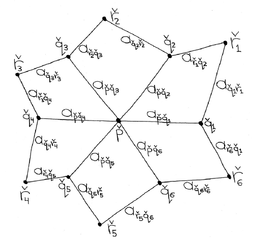
Figure 16. Although we will not consider umbilics on discrete surfaces in this text, it is possible to define umbilics on discrete isothermic surfaces, as follows: We now do not consider the discrete surface as a map from a domain in the integer lattice $\mathbb{Z}^{2}$ (it will not be). Let $\breve{p}$ be a vertex of a discrete surface consisting entirely of quadrilateral faces, with each face having concircular vertices. Thus all cross ratios on the faces are real, and we have a real cross ratio factorizing function $a$. Suppose that $\breve{p}$ is a vertex of some even number of faces, and at least six faces, of the surface. If the cross ratio factorizing condition in Definition 9.5 is satisfied, then we have a discrete isothermic surface with umbilic point $\breve{p}$. For example, if $\breve{p}$ has six adjacent faces as in the figure here, then we require that $a_{{\breve{q}}_{j-1}{\breve{r}}_{j-1}}=a_{{\breve{p}}{\breve{q}}_{j}}=a_{{\breve{r}}_{j}{\breve{q}}_{j+1}}$ for $j=2,3,4,5$, and also $a_{{\breve{q}}_{6}{\breve{r}}_{6}}=a_{{\breve{p}}{\breve{q}}_{1}}=a_{{\breve{r}}_{1}{\breve{q}}_{2}}$ and $a_{{\breve{q}}_{5}{\breve{r}}_{5}}=a_{{\breve{p}}{\breve{q}}_{6}}=a_{{\breve{r}}_{6}{\breve{q}}_{1}}$. Furthermore, this surface with an umbilic is then also discrete CMC if there exists a linear conserved quantity as in Definition 9.32.

9.2. Isothermicity from the perspective of smooth surfaces

One viewpoint on what a ”discrete isothermic surface” is, as in Definition 9.5, is as follows: Take a smooth surface $x$. Give it curvature line coordinates $x=x(u,v)$, so $x_{u}\perp x_{v}$. (Curvature line coordinates always exist away from umbilics.) Then the first and second fundamental forms are

$$I=\begin{pmatrix}g_{11}&0\\ 0&g_{22}\end{pmatrix}\;,\;\;\;II=\begin{pmatrix}b_{11}&0\\ 0&b_{22}\end{pmatrix}\;.$$

One can always stretch the coordinates, so that $x=x(u,v)=x(\tilde{u}(u),\tilde{v}(v))$ for any monotonic functions $\tilde{u}$ depending only on $u$, and $\tilde{v}$ depending only on $v$. Note that $\langle x_{\tilde{u}},x_{\tilde{v}}\rangle=0$, and $x_{\tilde{u}\tilde{v}}=x_{uv}\tfrac{du}{d\tilde{u}}\tfrac{dv}{d\tilde{v}}$ implies $\langle x_{\tilde{u}\tilde{v}},\vec{N}\rangle=0$, so $(\tilde{u},\tilde{v})$ are also curvature line coordinates. The surface is then isothermic if and only if there exist $\tilde{u}$, $\tilde{v}$ such that the metric becomes conformal, i.e. $\langle x_{\tilde{u}},x_{\tilde{u}}\rangle=\langle x_{\tilde{v}},x_{\tilde{v}}\rangle$, and this is equivalent to

$$\frac{g_{11}}{g_{22}}=\frac{a(u)}{b(v)}\;,$$

where the function $a$ depends only on $u$, and $b$ depends only on $v$.

Now consider the cross ratio $q_{\epsilon}$ of the four points $x(u,v)$, $x(u+\epsilon,v)$, $x(u+\epsilon,v+\epsilon)$ and $x(u,v+\epsilon)$. Using that $x_{u}\perp x_{v}$ implies $x_{u}x_{v}^{-1}=-x_{v}^{-1}x_{u}$, we see that

(9.3) $$\lim_{\epsilon\to 0}q_{\epsilon}=-\frac{g_{11}}{g_{22}}\;.$$

So $x$ is isothermic if and only if

(9.4) $$\lim_{\epsilon\to 0}q_{\epsilon}=-\frac{a(u)}{b(v)}\;,$$

where again $a$ is some function that depends only on $u$, and $b$ depends only on $v$. This description of isothermicity does not involve any stretching by $\tilde{u}$ or $\tilde{v}$, which we would not be able to do in the discrete case anyways, and now Definition 9.5 is a natural discretization of (9.4): The corresponding statement for discrete surfaces, where stretching of coordinates is no longer possible, is that the surface is discrete isothermic if and only if the cross ratio factorizing function can be chosen so that $a_{pq}=a_{rs}$ and $a_{ps}=a_{qr}$ for vertices $p,q,r,s$ (in order) about a given quadrilateral.

There is another perspective on isothermicity, coming from a lemma proven by Bobenko and Pinkall [20]:

Lemma 9.6.

Let $x(u,v)$ be a smooth surface in $\mathbb{R}^{3}$, and define the diagonal cross ratio

$$q_{\epsilon}^{d}=(x(u+\epsilon,v-\epsilon)-x(u-\epsilon,v-\epsilon))(x(u+\epsilon,v+\epsilon)-x(u+\epsilon,v-\epsilon))^{-1}\;\;\times$$

$$(x(u-\epsilon,v+\epsilon)-x(u+\epsilon,v+\epsilon))(x(u-\epsilon,v-\epsilon)-x(u-\epsilon,v+\epsilon))^{-1}\;.$$

Then

$$q_{\epsilon}^{d}=-1+\mathcal{O}(\epsilon)$$

if and only if $(u,v)$ are conformal coordinates for $x$, and

$$q_{\epsilon}^{d}=-1+\mathcal{O}(\epsilon^{2})$$

if and only if $(u,v)$ are isothermic coordinates for $x$.

The superscript ”$d$” in $q_{\epsilon}^{d}$ stands for ”diagonal”, because we are using diagonal elements to define this cross ratio, unlike with the previous $q_{\epsilon}$. Also, $\mathcal{O}(\epsilon^{k})$ denotes any function $f=f(\epsilon)$ such that the limit of $f(\epsilon)\epsilon^{-k}$, as $\epsilon$ approaches $0$, exists and is finite.

Proof.

Without loss of generality, we may assume $x(u,v)=\vec{0}$, and then for $\rho_{u},\rho_{v}\in\{\pm 1\}$, we have

$$x(u+\rho_{u}\epsilon,v+\rho_{v}\epsilon)=\epsilon\rho_{u}x_{u}+\epsilon\rho_{v}x_{v}+\tfrac{1}{2}\epsilon^{2}(x_{uu}+x_{vv}+2\rho_{u}\rho_{v}x_{uv})+\mathcal{O}(\epsilon^{3})\;,$$

so

$$q_{\epsilon}^{d}=x_{u}x_{v}^{-1}x_{u}x_{v}^{-1}+$$

$$\epsilon(x_{u}x_{v}^{-1}x_{uv}x_{v}^{-1}+x_{u}x_{v}^{-1}x_{u}x_{v}^{-1}x_{uv}x_{v}^{-1}-x_{uv}x_{v}^{-1}x_{u}x_{v}^{-1}-x_{u}x_{v}^{-1}x_{uv}x_{v}^{-1}x_{u}x_{v}^{-1})+\mathcal{O}(\epsilon^{2})\;.$$

If the coordinates are conformal, then $x_{u}x_{v}^{-1}x_{u}x_{v}^{-1}=-1$, and we have

$$q_{\epsilon}^{d}=-1+\epsilon x_{u}^{-4}(x_{u}x_{v}x_{uv}(x_{u}+x_{v})+x_{u}^{2}x_{uv}(x_{u}-x_{v}))+\mathcal{O}(\epsilon^{2})\;.$$

Now, if the coordinates are isothermic, then $b_{12}=0$, and so there exist scalar functions $A$ and $B$ so that

$$x_{uv}=Ax_{u}+Bx_{v}\;.$$

From this it follows that $q_{\epsilon}^{d}=-1+\epsilon\cdot 0+\mathcal{O}(\epsilon^{2})$. ∎

This lemma leads to the following definition for discrete isothermic surfaces in the narrow sense: $\mathfrak{f}$ is discrete isothermic if

$$q_{pqrs}=-1$$

for all quadrilaterals, with vertices $\mathfrak{f}_{p},\mathfrak{f}_{q},\mathfrak{f}_{r},\mathfrak{f}_{s}$.

However, with this definition, transformations, such as the Calapso transform, of isothermic surfaces will not remain isothermic. (Lemma 9.23 demonstrates this.) Hence the broader definition given in Definition 9.5 has been found to be more suitable.

One could think of a discrete surface $x$ with cross ratios exactly $-1$ as being ”isothermically parametrized”, while a discrete surface $\mathfrak{f}$ with cross ratios satisfying Definition 9.5 is one that could have its coordinates stretched so that it becomes isothermic, were it a smooth surface.

9.3. Moutard lifts for smooth surfaces

Given a smooth immersion $x(u,v)$ so that $x_{u}\perp x_{v}$, the light cone lift

$$X=X(u,v)=\begin{pmatrix}x&-x^{2}\\ 1&-x\end{pmatrix}\in PL^{4}$$

could also be represented by $\alpha\cdot X$ for any choice of nonzero real-valued function $\alpha=\alpha(u,v)$. If we choose $\alpha$ so that

(9.5) $$\partial_{u}\partial_{v}(\alpha X)||X\;,$$

or equivalently $\alpha_{u}x_{v}+\alpha_{v}x_{u}+\alpha x_{uv}=0$, then we say that $\alpha X$ is a Moutard lift.

Lemma 9.7.

Moutard lifts always exist for any smooth isothermic immersion.

Proof.

Let $x(u,v)$ be a smooth isothermic immersion with isothermic coordinates $u,v$. As we saw in the proofs of Lemma 8.47 and Lemma 9.6, there exist real-valued functions $A,B$ so that

$$x_{uv}=Ax_{u}+Bx_{v}\;.$$

Taking the inner product of this with $x_{u}$ and with $x_{v}$, and using that $\langle x_{u},x_{u}\rangle=\langle x_{v},x_{v}\rangle$ and $\langle x_{u},x_{v}\rangle=0$, we find that

$$A=\partial_{v}(\tfrac{1}{2}\log\langle x_{u},x_{u}\rangle)\;,\;\;\;B=\partial_{u}(\tfrac{1}{2}\log\langle x_{u},x_{u}\rangle)\;,$$

and thus it follows that $A_{u}=B_{v}$. The existence of a solution $\alpha$ to the equation $\alpha_{u}x_{v}+\alpha_{v}x_{u}+\alpha x_{uv}=0$ is equivalent to solving the system

$$\alpha_{u}=-\alpha B\;,\;\;\;\alpha_{v}=-\alpha A\;,$$

because $x_{uv}=Ax_{u}+Bx_{v}$. The compatibility condition of this system is $A_{u}=B_{v}$, seen as follows:

$$\alpha_{uv}=\alpha_{vu}$$

if and only if $(-\alpha B)_{v}=(-\alpha A)_{u}$, if and only if

$$\alpha_{v}B+\alpha B_{v}=\alpha_{u}A+\alpha A_{u}\;,$$

if and only if $(-\alpha A)B+\alpha B_{v}=(-\alpha B)A+\alpha A_{u}$, if and only if

$$B_{v}=A_{u}\>.$$

This proves the lemma. ∎

Remark 9.8.

Here is a hint of another way to prove Lemma 9.7: $x$ has isothermic coordinates, and so $e^{2\hat{u}}=\langle x_{u},x_{u}\rangle=\langle x_{v},x_{v}\rangle$ for some real-valued function $\hat{u}=\hat{u}(u,v)$, which implies $2\hat{u}_{u}e^{2\hat{u}}=2\langle x_{uv},x_{v}\rangle$, so $x_{uv}=*_{1}\cdot x_{u}+\hat{u}_{u}x_{v}+*_{2}\cdot\vec{N}$ for some functions $*_{j}$. Similarly, now taking the derivative of $e^{2\hat{u}}$ with respect to $v$, we have $x_{uv}=\hat{u}_{v}x_{u}+\hat{u}_{u}x_{v}+*_{2}\cdot\vec{N}$. Then $\langle x_{uv},\vec{N}\rangle=-\langle x_{u},\vec{N}_{v}\rangle=-\langle x_{u},*_{3}\cdot x_{v}\rangle=0$ implies $x_{uv}=\hat{u}_{v}x_{u}+\hat{u}_{u}x_{v}$. Then, taking the lift

$$X_{1}=X_{1}(u,v)=\begin{pmatrix}x&-x^{2}\\ 1&-x\end{pmatrix}$$

of $x=x(u,v)$ into $L^{4}$, we have $(X_{1})_{uv}=\hat{u}_{v}(X_{1})_{u}+\hat{u}_{u}(X_{1})_{v}$. We then rescale $X_{1}$ to $X_{2}:=e^{-\hat{u}}X_{1}$. A computation gives $(X_{2})_{uv}=\lambda\cdot X_{2}$ with $\lambda=\hat{u}_{u}\hat{u}_{v}-\hat{u}_{uv}$. $(X_{2})_{uv}=\lambda X_{2}$ is the condition for a Moutard lift. This argument would still hold if $(u,v)$ were just curvature line coordinates, but not necessarily isothermic coordinates, for the isothermic surface $x$. In other words, even if just $e^{2\hat{u}}=\langle x_{u},x_{u}\rangle\cdot\alpha=\langle x_{v},x_{v}\rangle\cdot\beta$, with functions $\alpha$ and $\beta$ such that $\alpha_{v}=\beta_{u}=0$, this is enough to say there exists a Moutard lift $X_{2}$, i.e. $(X_{2})_{uv}=\lambda X_{2}$.

9.4. Moutard lifts for discrete surfaces

Recall that for each point $\mathfrak{f}\in\text{Im}H$, there is a unique lift $F\in M_{\kappa}$ (not necessarily Moutard). However, as noted in Remark 8.1 and in the previous section, we can freely multiply $F$ by any nonzero real scalar, giving a scalar freedom in the choice of lift. Here, in the case of discrete surfaces, we describe particular choices for the lift $F$ that are convenient for computations, again called Moutard lifts, analogous to Moutard lifts for smooth surfaces.

Definition 9.9.

We say that $F$ is a Moutard lift if, for the four vertices $p,q,r,s$ listed in counterclockwise order about any quadrilateral, we have

$$(F_{r}-F_{p})||(F_{q}-F_{s})\;,$$

meaning that

(9.6) $$F_{r}-F_{p}=\mu(F_{q}-F_{s})$$

for some real scalar $\mu$.

The discrete Moutard equation as in Definition 9.9 can be justified as follows: consider a quadrilateral with lifts $F_{p}$, $F_{q}$, $F_{r}$ and $F_{s}$ at the vertices. The discrete second derivative of $F$ (analogous to $X_{uv}$ in the smooth case) is

$$(F_{r}-F_{s})-(F_{q}-F_{p})\;,$$

so the Moutard equation, i.e. the discrete version of Equation (9.5), can naturally be considered to be

$$F_{r}-F_{s}-F_{q}+F_{p}=\lambda_{1}\tfrac{1}{4}(F_{p}+F_{q}+F_{r}+F_{s})\;,\;\;\;\lambda_{1}\in\mathbb{R}\;,$$

and the $\tfrac{1}{4}$ can be absorbed into the $\lambda_{1}$ as $\lambda_{2}=\tfrac{1}{4}\lambda_{1}$. Then

$$F_{p}+F_{r}=\lambda(F_{q}+F_{s})\;,$$

where we have defined $\lambda$ by $\lambda=\tfrac{1+\lambda_{2}}{1-\lambda_{2}}$, i.e. $(F_{p}+F_{r})||(F_{q}+F_{s})$. Since $F_{*}$ is only projectively defined and thus signs of any of the $F_{*}$ can always be switched (i.e. $F_{*}\to-F_{*}$), we could also write

$$(F_{r}-F_{p})||(F_{q}-F_{s})$$

as in Definition 9.9.

Remark 9.10.

By a consideration similar to the one just above, we have discrete conjugate nets: A conjugate net for a smooth surface $x$ in $\mathbb{R}^{3}$ is coordinates so that the second fundamental form is diagonal (not necessarily conformal, nor necessarily curvature line coordinates), i.e. $x_{uv}\in\text{span}\{x_{u},x_{v}\}$. This last condition would be $(\mathfrak{f}_{r}-\mathfrak{f}_{s})-(\mathfrak{f}_{q}-\mathfrak{f}_{p})\in\text{span}\{\mathfrak{f}_{q}-\mathfrak{f}_{p},\mathfrak{f}_{s}-\mathfrak{f}_{p}\}$ for a discrete surface in $\mathbb{R}^{3}$, implying $\mathfrak{f}_{r}-\mathfrak{f}_{p}\in\text{span}\{\mathfrak{f}_{q}-\mathfrak{f}_{p},\mathfrak{f}_{s}-\mathfrak{f}_{p}\}$, and so $\mathfrak{f}_{p}$, $\mathfrak{f}_{q}$, $\mathfrak{f}_{r}$ and $\mathfrak{f}_{s}$ are coplanar. This is why we define discrete conjugate nets to be those discrete surfaces that have planar faces.

Lemma 9.11.

For a Moutard lift $F$ of a discrete isothermic surface $\mathfrak{f}$, the cross ratios $q_{pqrs}=\frac{a_{pq}}{a_{ps}}$ satisfy

$$q_{pqrs}=\frac{a_{pq}}{a_{ps}}=\frac{\langle F_{p},F_{q}\rangle}{\langle F_{p},F_{s}\rangle}\;.$$

Proof.

For Moutard lifts, since $||F_{r}||=||F_{p}||=0$, we have

$$0=\langle F_{r}+F_{p},F_{r}-F_{p}\rangle=\mu\langle F_{r}+F_{p},F_{q}-F_{s}\rangle\;,$$

and so $(F_{r}+F_{p})\perp(F_{q}-F_{s})$. Similarly, $(F_{r}-F_{p})\perp(F_{q}+F_{s})$. So

$$\langle F_{p},F_{r}\rangle\cdot\langle F_{q},F_{s}\rangle=\langle F_{p},F_{r}-F_{p}\rangle\cdot\langle F_{q}-F_{s},F_{s}\rangle=$$

$$\langle F_{p},\mu(F_{q}-F_{s})\rangle\cdot\langle\mu^{-1}(F_{r}-F_{p}),F_{s}\rangle=\langle F_{p},F_{q}-F_{s}\rangle\cdot\langle F_{r}-F_{p},F_{s}\rangle=$$

$$(\langle F_{p},F_{q}\rangle-\langle F_{p},F_{s}\rangle)\cdot(\langle F_{r},F_{s}\rangle-\langle F_{p},F_{s}\rangle)=(\langle F_{p},F_{q}\rangle-\langle F_{p},F_{s}\rangle)^{2}\;,$$

since $\langle F_{p},F_{q}\rangle=\langle F_{r},F_{s}\rangle$, by $(F_{r}+\epsilon F_{p})\perp(F_{q}-\epsilon F_{s})$ for $\epsilon=\pm 1$. Also, $\langle F_{q},F_{r}\rangle=\langle F_{p},F_{s}\rangle$. By Lemma 9.2 with the $p_{*}$ there being the projections of the $F_{*}$ here to $\text{Im}H$, and using that $\mathcal{E}=0$, we have proven the lemma. ∎

Remark 9.12.

The Moutard lift is not completely unique, and it has more than just the freedom of a constant scalar multiple. For example, if points $p$ corresponds to $(m,n)$ in the domain lattice in $\mathbb{Z}^{2}$, we could change a Moutard lift $F_{p}$ to $\alpha F_{p}$ when $m+n$ is even and $\beta F_{p}$ when $m+n$ is odd, for any nonzero constants $\alpha,\beta\in\mathbb{R}$, and this gives another Moutard lift.

Lemma 9.11 and Remark 9.12 imply that, by multiplying all $F_{p}$ by an appropriate constant real scalar, we may assume

(9.7) $$F_{p}F_{q}+F_{q}F_{p}=a_{pq}\cdot I$$

on all edges. Furthermore, any lift satisfying (9.7) is Moutard, and all Moutard lifts satisfy (9.7) up to the freedom given in Remark 9.12.

Remark 9.13.

Because $F_{p}F_{q}+F_{q}F_{p}$ is a scalar multiple of the identity, we sometimes ignore that it is a matrix, and simply consider it as that scalar $a_{pq}$.

Lemma 9.14.

Let $\mathfrak{f}\in\mathbb{R}^{3}\approx\text{Im}H$ be a discrete surface with concircular quadrilaterals. Then there exists a Moutard lift if and only if $\mathfrak{f}$ is isothermic. In particular, we can then choose the Moutard lift so that Equation (9.7) holds.

Proof.

First we assume $\mathfrak{f}$ is isothermic, and show that a Moutard lift exists. Choose a particular quadrilateral $pqrs$, and assume a lift $F$ is chosen so that (9.7) holds for both of the two edges $pq$ and $ps$ in that quadrilateral $pqrs$. Then Equation (9.2) implies we can choose $F_{r}$ to be (note that we are not requiring any condition like $F_{r}\in M_{\kappa}$ here)

$$F_{r}=F_{p}+\tfrac{1}{2}(\langle F_{q},F_{s}\rangle)^{-1}((a_{ps}-a_{pq})F_{q}+(a_{pq}-a_{ps})F_{s})\;.$$

Noting that isothermicity implies $a_{pq}=a_{rs}$ and $a_{ps}=a_{qr}$, a computation gives that (9.7) also holds on the edges $sr$ and $qr$. It follows that a Moutard lift exists.

We now assume that a Moutard lift $F$ exists, and then prove the surface $\mathfrak{f}$ is isothermic. Let $\mathfrak{f}_{p}$, $\mathfrak{f}_{q}$, $\mathfrak{f}_{r}$ and $\mathfrak{f}_{s}$ be the vertices of one quadrilateral of $\mathfrak{f}$ with cross ratio $q\in\mathbb{R}$. The assumption of concircularity implies that $F_{r}\in\text{span}\{F_{p},F_{q},F_{s}\}$, by Remark 9.4.

Now recall that a point

$$p\in\mathbb{R}^{3}\approx\text{Im}H$$

has lift

$$(x_{1},x_{2},x_{3},x_{4},x_{5})=(2p_{j},-(1-|p_{j}|^{2}),1+|p_{j}|^{2})\approx P_{j}=2\begin{pmatrix}p_{j}&-p_{j}^{2}\\ 1&-p_{j}\end{pmatrix}\in M_{0}\subseteq L^{4}\;,$$

where $\mathbb{R}^{3}=M_{0}$ is given by the $Q$ in (8.3) with $\kappa=0$.

We saw in (9.1) that for $p_{1},p_{2}\in\mathbb{R}^{3}\approx\text{Im}H$, we have

$$\langle P_{1},P_{2}\rangle=2(p_{1}-p_{2})^{2}\;.$$

We have $\mathfrak{f}_{p},\mathfrak{f}_{q},\mathfrak{f}_{r},\mathfrak{f}_{s}\in\text{Im}H$, and we can find $\alpha_{*}\in\mathbb{R}\setminus\{0\}$ so that $\alpha_{p}F_{p}$, $\alpha_{q}F_{q}$, $\alpha_{r}F_{r}$ and $\alpha_{s}F_{s}$ all lie in $M_{0}$, and then Lemma 8.37 gives that $q$ satisfies

(9.8) $$q^{2}=\left((\mathfrak{f}_{p}-\mathfrak{f}_{q})\frac{(\mathfrak{f}_{q}-\mathfrak{f}_{r})}{(\mathfrak{f}_{q}-\mathfrak{f}_{r})^{2}}(\mathfrak{f}_{r}-\mathfrak{f}_{s})\frac{(\mathfrak{f}_{s}-\mathfrak{f}_{p})}{(\mathfrak{f}_{s}-\mathfrak{f}_{p})^{2}}\right)^{2}=$$

$$=\frac{(\mathfrak{f}_{p}-\mathfrak{f}_{q})^{2}(\mathfrak{f}_{r}-\mathfrak{f}_{s})^{2}}{(\mathfrak{f}_{q}-\mathfrak{f}_{r})^{2}(\mathfrak{f}_{s}-\mathfrak{f}_{p})^{2}}=\frac{\langle\alpha_{p}F_{p},\alpha_{q}F_{q}\rangle\langle\alpha_{r}F_{r},\alpha_{s}F_{s}\rangle}{\langle\alpha_{q}F_{q},\alpha_{r}F_{r}\rangle\langle\alpha_{s}F_{s},\alpha_{p}F_{p}\rangle}=\frac{\langle F_{p},F_{q}\rangle\langle F_{r},F_{s}\rangle}{\langle F_{q},F_{r}\rangle\langle F_{s},F_{p}\rangle}\;.$$

A condition for $F_{r}$ to be in $L^{4}$ is, from Equation (9.6),

$$0=\langle F_{r},F_{r}\rangle=\langle\mu(F_{q}-F_{s})+F_{p},\mu(F_{q}-F_{s})+F_{p}\rangle=\mu^{2}\langle F_{q}-F_{s},F_{q}-F_{s}\rangle+2\mu\langle F_{q}-F_{s},F_{p}\rangle\;,$$

which implies

$$\mu=\frac{-2\langle F_{q}-F_{s},F_{p}\rangle}{\langle F_{q}-F_{s},F_{q}-F_{s}\rangle}\;,$$

and so

$$F_{r}=\frac{-2\langle F_{q}-F_{s},F_{p}\rangle}{\langle F_{q}-F_{s},F_{q}-F_{s}\rangle}(F_{q}-F_{s})+F_{p}\;,$$

which implies

$$\langle F_{r},F_{s}\rangle=\langle F_{p},F_{q}\rangle\;\;\;\text{and}\;\;\;\langle F_{r},F_{q}\rangle=\langle F_{p},F_{s}\rangle\;.$$

This shows that the cross ratios of $\mathfrak{f}$ satisfy the condition in Definition 9.5, completing the proof. ∎

Remark 9.15.

When the discrete surface is isothermic in the narrow sense, i.e. when the cross ratios are identically $-1$, there is a way to describe real values defined at the vertices so that they can be thought of as the ”scalar factor” or ”stretching factor” for the discrete ”conformal metric”, as follows: For a smooth surface $x(u,v)$ with isothermic coordinates $u,v$, we have as in Remark 9.8 that

$$X_{2}=e^{-\hat{u}}X_{1}$$

is a Moutard lift, where $e^{2\hat{u}}$ is the metric factor. Now, in the case of a discrete isothermic surface $\mathfrak{f}$, one lift is

$$F_{*}=\begin{pmatrix}f_{*}&-f_{*}^{2}\\ 1&-f_{*}\end{pmatrix}$$

($*$ now denotes vertices in the domain of $\mathfrak{f}$), and we can take a Moutard lift

$$\tilde{F}_{*}=s_{*}F_{*}$$

satisfying (9.7). Here $s_{*}$ will be the ”discrete metric”. We can take $a_{pq}=\pm 1$, and then

$$|a_{pq}|=2|\langle\tilde{F}_{p},\tilde{F}_{q}\rangle|$$

(i.e. $\tilde{F}_{*}$ is a Moutard lift satisfying (9.7)) implies

$$\tfrac{1}{2}=|s_{p}|\cdot|s_{q}|\cdot|\langle F_{p},F_{q}\rangle|=\tfrac{1}{2}|s_{p}|\cdot|s_{q}|\cdot|\mathfrak{f}_{p}-\mathfrak{f}_{q}|^{2}\;.$$

So $|s_{*}|$ behaves just like $e^{-\hat{u}}$ would in the case of a smooth isothermic surface.

We now give an application of Moutard lifts. Suppose that $(0,0)$, $(\pm 1,0)$, $(0,\pm 1)$, $\pm(1,1)$ and $\pm(1,-1)$ are all in the lattice domain of a discrete surface $\mathfrak{f}$. Then the diagonal vertex star of $\mathfrak{f}_{(0,0)}$ consists of the images $\mathfrak{f}_{(0,0)}$, $\mathfrak{f}_{(1,-1)}$, $\mathfrak{f}_{(1,1)}$, $\mathfrak{f}_{(-1,1)}$ and $\mathfrak{f}_{(-1,-1)}$ of the points $(0,0)$, $(1,-1)$, $(1,1)$, $(-1,1)$ and $(-1,-1)$. The proof of the next lemma applies Moutard lifts.

Lemma 9.16.

The five vertices of any diagonal vertex star on a discrete isothermic surface are cospherical.

Proof.

We can take the image $\mathfrak{f}_{(0,0)}$ of the point $(0,0)$ in the lattice domain to be the center of the diagonal vertex star. Let $F_{(i,j)}$ be a Moutard lift of $\mathfrak{f}_{(i,j)}$ satisfying Equation (9.7).

Our goal is to show

$$\text{dim}(F_{(0,0)},F_{(1,-1)},F_{(1,1)},F_{(-1,1)},F_{(-1,-1)})\leq 4\;.$$

Then there exists a spacelike vector $\mathcal{S}\in\mathbb{R}^{4,1}$ which produces the sphere $\tilde{\mathcal{S}}$, via (8.9), that contains all five points $F_{(0,0)},F_{(1,-1)},F_{(1,1)},F_{(-1,1)},F_{(-1,-1)}$, and the proof would be completed.

In the following computation, for the sake of simplicity, we ignore cases where some coefficients might be zero (those other cases can be dealt with separately).

Because we chose a Moutard lift, we have $\langle F_{q},F_{r}\rangle=\langle F_{p},F_{s}\rangle$ on any quadrilateral, implying

$$\langle F_{q},F_{p}-F_{r}\rangle=\langle F_{p},F_{q}-F_{s}\rangle\;,$$

so

$$\langle F_{q},F_{s}-F_{q}\rangle(F_{r}-F_{p})=\langle F_{q},F_{r}-F_{p}\rangle(F_{s}-F_{q})=\langle F_{p},F_{q}-F_{s}\rangle(F_{q}-F_{s})\;,$$

and so

$$\langle F_{q},F_{s}\rangle(F_{r}-F_{p})=-\frac{1}{2}(a_{pq}-a_{ps})(F_{q}-F_{s})\;.$$

This implies

$$\langle F_{(1,-1)},F_{(0,0)}\rangle(F_{(1,0)}-F_{(0,-1)})=-\frac{1}{2}(a_{(0,0)(1,0)}-a_{(0,-1)(0,0)})(F_{(1,-1)}-F_{(0,0)})\;,$$

$$\langle F_{(0,-1)},F_{(-1,0)}\rangle(F_{(0,0)}-F_{(-1,-1)})=-\frac{1}{2}(a_{(-1,0)(0,0)}-a_{(0,-1)(0,0)})(F_{(0,-1)}-F_{(-1,0)})\;,$$

$$\langle F_{(0,0)},F_{(-1,1)}\rangle(F_{(0,1)}-F_{(-1,0)})=-\frac{1}{2}(a_{(-1,0)(0,0)}-a_{(0,0)(0,1)})(F_{(0,0)}-F_{(-1,1)})\;,$$

$$\langle F_{(1,0)},F_{(0,1)}\rangle(F_{(1,1)}-F_{(0,0)})=-\frac{1}{2}(a_{(0,0)(1,0)}-a_{(0,0)(0,1)})(F_{(1,0)}-F_{(0,1)})\;,$$

and then

$$F_{(1,0)}-F_{(0,-1)}=-\frac{a_{(0,0)(1,0)}-a_{(0,-1)(0,0)}}{2\langle F_{(1,-1)},F_{(0,0)}\rangle}(F_{(1,-1)}-F_{(0,0)})\;,$$

$$F_{(0,-1)}-F_{(-1,0)}=\frac{-2\langle F_{(0,-1)},F_{(-1,0)}\rangle}{a_{(-1,0)(0,0)}-a_{(0,-1)(0,0)}}(F_{(0,0)}-F_{(-1,-1)})\;,$$

$$F_{(-1,0)}-F_{(0,1)}=\frac{a_{(-1,0)(0,0)}-a_{(0,0)(0,1)}}{2\langle F_{(-1,1)},F_{(0,0)}\rangle}(F_{(0,0)}-F_{(-1,1)})\;,$$

$$F_{(0,1)}-F_{(1,0)}=\frac{2\langle F_{(1,0)},F_{(0,1)}\rangle}{a_{(0,0)(1,0)}-a_{(0,0)(0,1)}}(F_{(1,1)}-F_{(0,0)})\;.$$

Adding these last four equations, we see that a linear combination of those five points $F_{(0,0)},F_{(1,-1)},F_{(1,1)},F_{(-1,1)},F_{(-1,-1)}$ equals zero, proving the result. ∎

The conclusion of Lemma 9.16 is in fact equivalent to the discrete surface being isothermic, and this then makes it obvious that discrete isothermicity is invariant under Möbius transformations.

Definition 9.17.

We say that the sphere (containing the vertex star) in Lemma 9.16 is the central sphere of the discrete isothermic surface at the central vertex of the diagonal vertex star.

9.5. Christoffel transforms

When $\mathfrak{f}$ is a discrete isothermic surface in $\mathbb{R}^{3}\approx\text{Im}H$, we can define the Christoffel transform $\mathfrak{f}^{*}$ (also in $\mathbb{R}^{3}$) of $\mathfrak{f}$ as follows:

Definition 9.18.

Let $\mathfrak{f}$ be a discrete isothermic surface in $\mathbb{R}^{3}$. Then the Christoffel transform $\mathfrak{f}^{*}$ of $\mathfrak{f}$ satisfies

(9.9) $$d\mathfrak{f}_{pq}^{*}d\mathfrak{f}_{pq}=a_{pq}\;.$$

Here, for any object $\mathfrak{F}$ defined on vertices, $d\mathfrak{F}_{pq}$ denotes the difference

$$d\mathfrak{F}_{pq}:=\mathfrak{F}_{q}-\mathfrak{F}_{p}$$

of the values of $\mathfrak{F}$ at the vertices $q$ and $p$.

To see that this definition is natural, we consider the Christoffel transform $x^{*}$ of a smooth surface $x$ in $\mathbb{R}^{3}$ with isothermic coordinates $u,v$. In the smooth case, we may assume $x$ and $x^{*}$ satisfy

$$dx=x_{u}du+x_{v}dv\;,\;\;\;dx^{*}=x_{u}^{-1}du-x_{v}^{-1}dv\;,$$

as seen in the previous chapter. So

$$dx^{*}(\partial_{u})dx(\partial_{u})=1\;\;\;\text{and}\;\;\;dx^{*}(\partial_{v})dx(\partial_{v})=-1\;.$$

We also have

$$\lim_{\epsilon\to 0}q_{\epsilon}=-1=\frac{dx^{*}(\partial_{u})dx(\partial_{u})}{dx^{*}(\partial_{v})dx(\partial_{v})}\;,$$

by Equation (9.3). In the discrete case, we loosened the $-1$ in the right-hand side of Equation (9.3) to the $a_{pq}/a_{ps}$ in the right-hand side of $q_{pqrs}=a_{pq}/a_{ps}$, as in Definition 9.5. Because of this, it is natural to consider that

$$\frac{a_{pq}}{a_{ps}}=\frac{d\mathfrak{f}^{*}_{pq}d\mathfrak{f}_{pq}}{d\mathfrak{f}^{*}_{ps}d\mathfrak{f}_{ps}}\;,$$

where $d\mathfrak{f}_{pq}$, $d\mathfrak{f}^{*}_{pq}$, $d\mathfrak{f}_{ps}$, $d\mathfrak{f}^{*}_{ps}$ now represent discrete analogs of $dx(\partial_{u})$, $dx^{*}(\partial_{u})$, $dx(\partial_{v})$, $dx^{*}(\partial_{v})$, and so Definition 9.18 becomes natural.

We can then prove the following:

Lemma 9.19.

[19] If $\mathfrak{f}$ is a discrete isothermic surface, then there exists a Christoffel transform $\mathfrak{f}^{*}$ of $\mathfrak{f}$.

Proof.

$\mathfrak{f}^{*}$ exists if and only if the compatibility condition

(9.10) $$d\mathfrak{f}^{*}_{pq}+d\mathfrak{f}^{*}_{qr}=d\mathfrak{f}^{*}_{ps}+d\mathfrak{f}^{*}_{sr}$$

holds, that is to say, we can apply “discrete integration” of $d\mathfrak{f}^{*}$ to obtain $\mathfrak{f}^{*}$.

We now prove that Equation (9.10) holds with $d\mathfrak{f}^{*}$ defined as in Equation (9.9). By Equation (9.9), Equation (9.10) is equivalent to

$$a_{pq}d\mathfrak{f}_{pq}^{-1}+a_{qr}d\mathfrak{f}_{qr}^{-1}=a_{ps}d\mathfrak{f}_{ps}^{-1}+a_{sr}d\mathfrak{f}_{sr}^{-1}\;.$$

Because $a_{pq}=a_{sr}$ and $a_{ps}=a_{qr}$ (by isothermicity), this equation is equivalent to

$$\frac{a_{pq}}{a_{ps}}(d\mathfrak{f}_{pq}^{-1}-d\mathfrak{f}_{sr}^{-1})=d\mathfrak{f}_{ps}^{-1}-d\mathfrak{f}_{qr}^{-1}\;.$$

By Lemma 8.37, the cross ratio is $a_{pq}a_{ps}^{-1}=d\mathfrak{f}_{pq}d\mathfrak{f}_{qr}^{-1}d\mathfrak{f}_{rs}d\mathfrak{f}_{sp}^{-1}=d\mathfrak{f}_{qr}^{-1}d\mathfrak{f}_{rs}d\mathfrak{f}_{sp}^{-1}d\mathfrak{f}_{pq}=d\mathfrak{f}_{qr}^{-1}d\mathfrak{f}_{pq}d\mathfrak{f}_{sp}^{-1}d\mathfrak{f}_{rs}$, and so the equation becomes

$$d\mathfrak{f}_{qr}^{-1}d\mathfrak{f}_{rs}d\mathfrak{f}_{sp}^{-1}+d\mathfrak{f}_{qr}^{-1}d\mathfrak{f}_{pq}d\mathfrak{f}_{sp}^{-1}=d\mathfrak{f}_{ps}^{-1}-d\mathfrak{f}_{qr}^{-1}\;,$$

that is, $d\mathfrak{f}^{-1}_{qr}(d\mathfrak{f}_{rs}+d\mathfrak{f}_{pq})d\mathfrak{f}^{-1}_{sp}=d\mathfrak{f}^{-1}_{ps}-d\mathfrak{f}^{-1}_{qr}$, i.e.

$$d\mathfrak{f}_{rs}+d\mathfrak{f}_{pq}+d\mathfrak{f}_{qr}+d\mathfrak{f}_{sp}=0\;,$$

and this follows from the fact that $\mathfrak{f}$ exists and so $d\mathfrak{f}$ is closed. ∎

Lemma 9.20.

Let $\mathfrak{f}$ be a discrete isothermic surface. Then the Christoffel transform $\mathfrak{f}^{*}$ of $\mathfrak{f}$ is isothermic with the same cross ratios as $\mathfrak{f}$.

Proof.

Let $q,q^{*}$ be the cross ratios of $\mathfrak{f}$, $\mathfrak{f}^{*}$ respectively. Then

$$q^{*}=d\mathfrak{f}_{pq}^{*}(d\mathfrak{f}_{qr}^{*})^{-1}d\mathfrak{f}_{rs}^{*}(d\mathfrak{f}_{sp}^{*})^{-1}=a_{pq}d\mathfrak{f}_{pq}^{-1}(a_{qr}d\mathfrak{f}_{qr}^{-1})^{-1}a_{rs}d\mathfrak{f}_{rs}^{-1}(a_{sp}d\mathfrak{f}_{sp}^{-1})^{-1}=$$

$$(a_{pq}/a_{qr})(a_{rs}/a_{sp})d\mathfrak{f}_{pq}^{-1}(d\mathfrak{f}_{qr}^{-1})^{-1}d\mathfrak{f}_{rs}^{-1}(d\mathfrak{f}_{sp}^{-1})^{-1}=q^{2}(d\mathfrak{f}_{sp}^{-1}d\mathfrak{f}_{rs}d\mathfrak{f}_{qr}^{-1}d\mathfrak{f}_{pq})^{-1}\;.$$

Then Lemma 8.37 implies

$$q^{*}=q^{2}(d\mathfrak{f}_{pq}d\mathfrak{f}_{qr}^{-1}d\mathfrak{f}_{rs}d\mathfrak{f}_{sp}^{-1})^{-1}=q^{2}\cdot q^{-1}=q\;.$$

∎

9.6. Calapso transforms

Like in the smooth case, we can define Calapso transformations $T$ in the discrete case. We first define $\tau$ as

$$\tau_{pq}=\begin{pmatrix}\mathfrak{f}_{p}\\ 1\end{pmatrix}(\mathfrak{f}_{q}^{*}-\mathfrak{f}_{p}^{*})\begin{pmatrix}1&-\mathfrak{f}_{q}\end{pmatrix}\;.$$

Note that $\tau_{pq}$ does not have symmetry with respect to $p$ and $q$, and this was just a choice that was made, and there is no particular geometric motivation for choosing $\mathfrak{f}_{p}$ in the leftward vector and $\mathfrak{f}_{q}$ in the rightward vector. Then taking any lift

$$F_{p}=\alpha_{p}\begin{pmatrix}\mathfrak{f}_{p}&-\mathfrak{f}_{p}^{2}\\ 1&-\mathfrak{f}_{p}\end{pmatrix}$$

at all $p$, a short computation gives

(9.11) $$\tau_{pq}=\begin{pmatrix}\mathfrak{f}_{p}d\mathfrak{f}_{pq}^{*}&-\mathfrak{f}_{p}d\mathfrak{f}_{pq}^{*}\mathfrak{f}_{q}\\ d\mathfrak{f}_{pq}^{*}&-d\mathfrak{f}_{pq}^{*}\mathfrak{f}_{q}\end{pmatrix}=-a_{pq}\frac{F_{p}F_{q}}{F_{p}F_{q}+F_{q}F_{p}}\;.$$

Note that, although $F_{p}F_{q}+F_{q}F_{p}$ is a matrix, we are regarding it as a scalar here, like in Remark 9.13.

If $F$ is a Moutard lift, then we can assume (9.7), and so we have

(9.12) $$\tau_{pq}=-F_{p}F_{q}\;.$$

For adjacent vertices $p,q$, we define $T=T^{\lambda}$ by

(9.13) $$T_{q}=T_{p}(I+\lambda\tau_{pq})\;.$$

This is not a commutative operation, as we will see in the proof of the next lemma, i.e. we cannot switch $p$ and $q$ and expect this equation to still hold. So we must decide on a direction for each edge. Let us do this by fixing one vertex p and then for any edge $\hat{p}\hat{q}$, where $\hat{q}$ is farther from $p$ than $\hat{p}$ is, apply the above equation to define $T_{\hat{q}}=T_{\hat{p}}(I+\lambda\tau_{\hat{p}\hat{q}})$. It will turn out that this noncommutativity will not affect the Calapso transform (see the definition of the Calapso transform below), because $T$ is in fact defined up to real scalar factors even without this normalization of directions, so it is not a problem, but let us normalize these directions that we use in (9.13) in order to choose a particular $T$. (We will also use this normalization in the proofs of Lemmas 9.23 and 9.25.)

A direct computation shows that $I+\lambda\tau_{pq}$ (with $a,b,c,d$ now regarded as the entries in the matrix $I+\lambda\tau_{pq}$) satisfies (8.18) and (8.19) when $1-\lambda a_{pq}\neq 0$, so $I+\lambda\tau_{pq}\in\text{Mob}(3)$ and then $T$ is as well, when the initial condition chosen for the solution $T$ is taken in $\text{Mob}(3)$.

Definition 9.21.

We say that $TFT^{-1}$ is a Calapso transform.

We can write $TFT^{-1}$ as $T_{p}F_{p}T_{p}^{-1}$ when we wish to specify which vertex $p$ is being used, and as $T^{\lambda}F(T^{\lambda})^{-1}$ when we wish to specify which value of $\lambda$ has been chosen.

We will see in the proof of the next lemma that $T$ is only defined up to real scalar factors, i.e. the $T$ are actually multivalued, and become well defined only when considered in a projectivized space. But, as noted above, this freedom does not affect the resulting Calapso transform $TFT^{-1}$.

Lemma 9.22.

If $\mathfrak{f}$ is a discrete isothermic surface, then a solution $T\in\text{Mob}(3)$ to (9.13) exists.

Proof.

First we note that

$$(I+\lambda\tau_{pq})(I+\lambda\tau_{qp})$$

is a real scalar multiple of $I$, so that $T$ is defined up to a real scalar factor when applying (9.13) back and forth along a single edge. To see this, we need to see that

$$\tau_{pq}+\tau_{qp}$$

is a real scalar multiple of $I$. Taking a Moutard lift $F$ of $\mathfrak{f}$ so that (9.7) holds, $\tau_{pq}+\tau_{qp}=-F_{p}F_{q}-F_{q}F_{p}=-a_{pq}I$ is a real scalar multiple of $I$.

For a quadrilateral with vertices $p,q,r,s$ in counterclockwise order, we have, if $T$ exists, that

$$T_{r}=T_{q}(I+\lambda\tau_{qr})=T_{p}(I+\lambda\tau_{pq})(I+\lambda\tau_{qr})=$$

$$T_{p}(I+\lambda\tau_{ps})(I+\lambda\tau_{sr})\;.$$

So existence of $T$ would be implied by

(9.14) $$(I+\lambda\tau_{pq})(I+\lambda\tau_{qr})=(I+\lambda\tau_{ps})(I+\lambda\tau_{sr})\;,$$

that is to say, we want to show

$$\tau_{pq}\tau_{qr}=\tau_{ps}\tau_{sr}$$

and

$$\tau_{pq}+\tau_{qr}-\tau_{sr}-\tau_{ps}=0\;.$$

The first of these two equations follows immediately from

$$\begin{pmatrix}1&-\mathfrak{f}_{q}\end{pmatrix}\begin{pmatrix}\mathfrak{f}_{q}\\ 1\end{pmatrix}=0\;,$$

and the second one is not difficult to show if we use a Moutard lift satisfying (9.12): Using such a lift $F$ means that we need only show

$$F_{p}F_{q}+F_{q}F_{r}=F_{p}F_{s}+F_{s}F_{r}\;,$$

i.e. that

$$F_{p}(F_{q}-F_{s})+(F_{q}-F_{s})F_{r}=0\;.$$

But by definition of the Moutard lift, $F_{q}-F_{s}$ and $F_{p}-F_{r}$ are parallel, so we need only show

$$F_{p}(F_{p}-F_{r})+(F_{p}-F_{r})F_{r}=0\;.$$

This is clearly true, since $F_{p}^{2}=F_{r}^{2}=0$.

Finally, as noted before, if $T_{p_{0}}\in\text{Mob(3)}$ at one vertex $p_{0}$, and $1-\lambda a_{pq}$ is never zero, then $T_{p}\in\text{Mob}(3)$ for all vertices $p$. ∎

Lemma 9.23.

Let $\mathfrak{f}$ be a discrete isothermic surface with lift $F$. The Calapso transform $F_{p}\to F_{p}^{\mu}:=T_{p}^{\mu}F_{p}(T_{p}^{\mu})^{-1}$ gives another isothermic surface $\mathfrak{f}^{\mu}$, and the cross ratio factorizing function $a_{pq}$ changes from $\mathfrak{f}$ to $\mathfrak{f}^{\mu}$ as follows:

$$a_{pq}\to a_{pq}^{\mu}=\frac{a_{pq}}{1-\mu a_{pq}}\;.$$

Proof.

Let $F$ be a Moutard lift satisfying (9.7). For a quadrilateral with vertices $p$, $q$, $r$ and $s$ listed in counterclockwise order around the quadrilateral, and noting that

$$(I+\lambda\tau_{pq})(I+\lambda\tau_{qp})=(1-\lambda a_{pq})I\;,$$

we have (assume $pq$ is directed from $p$ to $q$)

$$\langle F_{p}^{\lambda},F_{q}^{\lambda}\rangle=\langle T_{p}F_{p}T_{p}^{-1},T_{q}F_{q}T_{q}^{-1}\rangle=$$

$$\tfrac{-1}{2}[T_{p}F_{p}(I+\lambda\tau_{pq})F_{q}T_{q}^{-1}+\frac{1}{1-\lambda a_{pq}}T_{q}F_{q}(I+\lambda\tau_{qp})F_{p}T_{p}^{-1}]=$$

$$\tfrac{-1}{2}[T_{p}F_{p}F_{q}T_{q}^{-1}+\frac{1}{1-\lambda a_{pq}}T_{q}F_{q}F_{p}T_{p}^{-1}]=$$

$$\tfrac{-1}{2}T_{p}[F_{p}F_{q}\frac{1}{1-\lambda a_{pq}}\cdot I+\frac{1}{1-\lambda a_{pq}}I\cdot F_{q}F_{p}]T_{p}^{-1}=\frac{1}{1-\lambda a_{pq}}\langle F_{p},F_{q}\rangle\;.$$

Also (assume as well that $qr$ is directed from $q$ to $r$),

$$\langle F_{p}^{\lambda},F_{r}^{\lambda}\rangle=\langle T_{p}F_{p}T_{p}^{-1},T_{r}F_{r}T_{r}^{-1}\rangle=\tfrac{-1}{2}\left[T_{p}F_{p}T_{p}^{-1}T_{r}F_{r}T_{r}^{-1}+T_{r}F_{r}T_{r}^{-1}T_{p}F_{p}T_{p}^{-1}\right]=$$

$$\tfrac{-1}{2}\left[T_{p}F_{p}T_{p}^{-1}T_{q}T_{q}^{-1}T_{r}F_{r}T_{r}^{-1}+T_{r}F_{r}T_{r}^{-1}T_{q}T_{q}^{-1}T_{p}F_{p}T_{p}^{-1}\right]=$$

$$\tfrac{-1}{2}\left[T_{p}F_{p}\cdot I\cdot I\cdot F_{r}T_{r}^{-1}+\frac{1}{1-\lambda a_{pq}}\frac{1}{1-\lambda a_{qr}}T_{r}F_{r}F_{p}T_{p}^{-1}\right]=$$

$$\tfrac{-1}{2}T_{q}\left[T_{q}^{-1}T_{p}F_{p}F_{r}T_{r}^{-1}T_{q}+\frac{1}{1-\lambda a_{pq}}\frac{1}{1-\lambda a_{qr}}T_{q}^{-1}T_{r}F_{r}F_{p}T_{p}^{-1}T_{q}\right]T_{q}^{-1}=$$

$$\frac{1}{1-\lambda a_{pq}}\frac{1}{1-\lambda a_{qr}}\langle F_{p},F_{r}\rangle\;.$$

Similarly,

$$\langle F_{p}^{\lambda},F_{s}^{\lambda}\rangle=\frac{1}{1-\lambda a_{ps}}\langle F_{p},F_{s}\rangle\;,$$

$$\langle F_{q}^{\lambda},F_{r}^{\lambda}\rangle=\frac{1}{1-\lambda a_{qr}}\langle F_{q},F_{r}\rangle\;,$$

$$\langle F_{q}^{\lambda},F_{s}^{\lambda}\rangle=\frac{1}{1-\lambda a_{pq}}\frac{1}{1-\lambda a_{qr}}\langle F_{q},F_{s}\rangle\;.$$

We now renotate the subscripts $p,q,r,s$ by $p_{1},p_{2},p_{3},p_{4}$, respectively. Then, using the lift $F$ satisfying (9.7) chosen here in Lemma 9.2 (note that we do not need to require $F\in M_{\kappa}$), and noting that we have $s_{12}=s_{34}=-\tfrac{1}{2}a_{p_{1}p_{2}}$ and $s_{14}=s_{23}=-\tfrac{1}{2}a_{p_{1}p_{4}}$, and because $q=a_{p_{1}p_{2}}/a_{p_{1}p_{4}}$, Lemma 9.2 implies $s_{13}s_{24}=\tfrac{1}{4}(a_{p_{1}p_{2}}-a_{p_{1}p_{4}})^{2}$. A computation, again using Lemma 9.2, then shows that the corresponding cross ratio on the Christoffel transform $\mathfrak{f}^{\mu}$ is

$$a_{pq}^{\mu}/a_{ps}^{\mu}\;,$$

where

$$a_{pq}^{\mu}=\frac{a_{pq}}{1-\mu a_{pq}}\;,\;\;\;a_{ps}^{\mu}=\frac{a_{ps}}{1-\mu a_{ps}}\;.$$

Thus $\mathfrak{f}^{\mu}$ is an isothermic surface, and the lemma is proven. ∎

In the above proof we saw that $\langle F_{p}^{\mu},F_{q}^{\mu}\rangle=(1-\mu a_{pq})^{-1}\langle F_{p},F_{q}\rangle=-\tfrac{1}{2}a_{pq}^{\mu}$ and $\langle F_{p}^{\mu},F_{s}^{\mu}\rangle=(1-\mu a_{ps})^{-1}\langle F_{p},F_{s}\rangle=-\tfrac{1}{2}a_{ps}^{\mu}$, so this corollary follows:

Corollary 9.24.

If $F_{p}$ is a Moutard lift of a discrete isothermic surface $\mathfrak{f}$ satisfying (9.7), then so is $F_{p}^{\mu}$, for any $\mu\in\mathbb{R}\setminus\{0\}$.

In order to state the next lemma, we define $T^{\lambda,\mu}$ by

$$T^{\lambda,\mu}_{q}=T^{\lambda,\mu}_{p}(I+\mu\tau_{pq}^{\lambda})\;,$$

where

$$\tau_{pq}^{\lambda}=\frac{-a_{pq}^{\lambda}F_{p}^{\lambda}F_{q}^{\lambda}}{F_{p}^{\lambda}F_{q}^{\lambda}+F_{q}^{\lambda}F_{p}^{\lambda}}\;,\;\;\;a_{pq}^{\lambda}=\frac{a_{pq}}{1-\lambda a_{pq}}\;,\;\;\;F_{p}^{\lambda}=T_{p}^{\lambda}F_{p}(T_{p}^{\lambda})^{-1}\;.$$

Lemma 9.25.

Let $\mathfrak{f}$ be a discrete isothermic surface with associated $T$. Then $T$ is a 1-parameter group, that is, we can choose $T^{\lambda,\mu}$ so that

$$T^{\mu+\lambda}=T^{\lambda,\mu}T^{\lambda}$$

for any $\lambda,\mu\in\mathbb{R}$.

Proof.

Without loss of generality, assume $F$ is a Moutard lift satisfying (9.7), and so Corollary 9.24 implies $\tau_{pq}^{\lambda}=-F_{p}^{\lambda}F_{q}^{\lambda}$. First note that $T_{q}^{\lambda}=T_{p}^{\lambda}(I+\lambda\tau_{pq})$. We wish to show $T^{\mu+\lambda}=T^{\lambda,\mu}T^{\lambda}$, i.e.

(9.15) $$T^{\lambda,\mu}_{q}T_{q}^{\lambda}=T^{\lambda,\mu}_{p}T^{\lambda}_{p}(I+(\mu+\lambda)\tau_{pq})\;,$$

where the edge $pq$ is directed from $p$ to $q$. Note that

(9.16) $$(T_{p}^{\lambda})^{-1}T_{q}^{\lambda}=I+\lambda\tau_{pq}\;,$$

and inverting gives

(9.17) $$(T_{q}^{\lambda})^{-1}T_{p}^{\lambda}=\frac{1}{1-\lambda a_{pq}}(I+\lambda\tau_{qp})\;,$$

since $F$ is a Moutard lift satisfying (9.7). Then

$$T^{\lambda,\mu}_{q}T_{q}^{\lambda}=T^{\lambda,\mu}_{p}(I-\mu F_{p}^{\lambda}F_{q}^{\lambda})T_{q}^{\lambda}=$$

$$=T^{\lambda,\mu}_{p}(I-\mu T_{p}^{\lambda}F_{p}(T_{p}^{\lambda})^{-1}T_{q}^{\lambda}F_{q}(T_{q}^{\lambda})^{-1})T_{q}^{\lambda}\;.$$

Then, using the properties $F_{p}\tau_{pq}=\tau_{pq}F_{q}=0$ and (9.16), we have

$$T^{\lambda,\mu}_{q}T_{q}^{\lambda}=T_{p}^{\lambda,\mu}(I+\mu T_{p}^{\lambda}\tau_{pq}(T_{q}^{\lambda})^{-1})T_{q}^{\lambda}=$$

$$=T_{p}^{\lambda,\mu}T_{p}^{\lambda}((T_{p}^{\lambda})^{-1}T_{q}^{\lambda}+\mu\tau_{pq})=T_{p}^{\lambda,\mu}T_{p}^{\lambda}((I+\lambda\tau_{pq})+\mu\tau_{pq})=$$

$$=T_{p}^{\lambda,\mu}T_{p}^{\lambda}(I+(\lambda+\mu)\tau_{pq})\;.$$

Thus we have shown (9.15). ∎

Now we recall that, for general lifts $F$ that are not necessarily Moutard, we have

$$\tau_{pq}=\frac{-a_{pq}F_{p}F_{q}}{F_{p}F_{q}+F_{q}F_{p}}\;,\;\;\;\tau_{pq}^{\mu}=\frac{-a_{pq}^{\mu}F_{p}^{\mu}F_{q}^{\mu}}{F_{p}^{\mu}F_{q}^{\mu}+F_{q}^{\mu}F_{p}^{\mu}}\;,$$

and, by Equations (9.16) and (9.17), we have

(9.18) $$(I+\mu\tau_{pq})^{-1}=\frac{1}{1-\mu a_{pq}}(I+\mu\tau_{qp})\;.$$

Remark 9.26.

Equation (9.18) is not symmetric in $p$ and $q$. In fact, as noted before, $\tau$ itself is not symmetric in $p$ and $q$. However, the most essential object, the family of flat connections $\Gamma_{pq}^{\lambda}$, is symmetric in $p$ and $q$ (see Remark 9.29). We will discuss flat connections in the next Section 9.7.

Furthermore, if $F$ is Moutard satisfying (9.7), this is true of $F^{\mu}$ as well, by Corollary 9.24, and we have $\tau_{pq}^{\mu}=-F_{p}^{\mu}F_{q}^{\mu}=-T_{p}^{\mu}F_{p}(T_{p}^{\mu})^{-1}T_{q}^{\mu}F_{q}(T_{q}^{\mu})^{-1}=-T_{p}^{\mu}F_{p}(I+\mu\tau_{pq})F_{q}(T_{q}^{\mu})^{-1}=T_{p}^{\mu}(-F_{p}F_{q})(T_{q}^{\mu})^{-1}$, so we have

(9.19) $$\tau_{pq}^{\mu}=T_{p}^{\mu}\tau_{pq}(T_{q}^{\mu})^{-1}\;.$$

This equation will be used later, when we show that if $\mathfrak{f}$ has a polynomial conserved quantity of type $n$, then so do its Calapso transformations (see Lemma 11.26). In particular, if $\mathfrak{f}$ is a discrete isothermic CMC surface in some space form, then so are its Calapso transformations (in different space forms in general). But since we have not defined the notions of polynomial conserved quantities and discrete CMC surfaces yet, we come back to this later.

9.7. Flat connections

Let us first review what a connection is in the smooth case. We will see how isothermic surfaces have a 1-parameter family of flat connections. Although we do not show it here (see [30] for such an argument), the converse is also true: existence of a family of flat connections implies that the surface is isothermic.

Recall that the Riemannian connection of a Riemannian manifold is the unique connection satisfying

(9.20) $$\nabla_{fX+Y}Z=f\nabla_{X}Z+\nabla_{Y}Z\;,$$

(9.21) $$\nabla_{X}(fY+Z)=X(f)Y+f\nabla_{X}Y+\nabla_{X}Z\;,$$

(9.22) $$\nabla_{X}Y-\nabla_{Y}X=[X,Y]\;,$$

(9.23) $$X\langle Y,Z\rangle=\langle\nabla_{X}Y,Z\rangle+\langle Y,\nabla_{X}Z\rangle\;,$$

where $X,Y,Z$ are any smooth tangent vector fields of the manifold, and $f$ is any smooth function from the manifold to $\mathbb{R}$. The first two relations (9.20), (9.21) define general affine connections, and adding in the last two conditions (9.22), (9.23) makes the connection a Riemannian connection.

Taking an $n$-dimensional manifold $M^{n}$ with affine connection $\nabla$, and taking a basis $X_{1}$, $X_{2}$, … , $X_{n}$ of vector fields for the tangent spaces, we define $\Gamma_{ij}^{k}$ and $R_{lij}^{k}$ by

$$\nabla_{X_{i}}X_{j}=\sum_{k=1}^{n}\Gamma_{ij}^{k}X_{k}\;,$$

(9.24) $$\nabla_{X_{i}}\nabla_{X_{j}}X_{l}-\nabla_{X_{j}}\nabla_{X_{i}}X_{l}-\nabla_{[X_{i},X_{j}]}X_{l}=\sum_{k=1}^{n}R_{lij}^{k}X_{k}\;.$$

We define the one forms $\omega^{i}$ and $\omega_{j}^{i}$ by (here $\delta_{j}^{i}$ is the Kronecker delta function)

$$\omega^{i}(X_{j})=\delta_{j}^{i}\;,\;\;\;\omega_{j}^{i}=\sum_{k=1}^{n}\Gamma_{kj}^{i}\omega^{k}\;.$$

The one forms $\omega_{j}^{i}$ are called the connection one forms. Then

$$d\omega_{l}^{i}+\sum_{p=1}^{n}\omega_{p}^{i}\wedge\omega_{l}^{p}=\tfrac{1}{2}\sum_{j,k=1}^{n}R_{ljk}^{i}\omega^{j}\wedge\omega^{k}\;.$$

When the connection is the Riemannian connection, the $R_{ljk}^{i}$ give the Riemannian curvature tensor. When, for an affine connection, all of the $R_{ljk}^{i}$ are zero, then we say that $\nabla$ is a flat connection. For a more thorough explanation of the above equations, there are many textbooks one could look at, for example [70].

For a smooth isothermic surface $x$, we can regard $\mathbb{R}^{4,1}$ as $5$-dimensional fibers of a trivial vector bundle defined on $x$. We now define $\nabla=d+\lambda\tau$ for any choice of $\lambda\in\mathbb{R}$, i.e.

(9.25) $$\nabla_{Z}Y=d_{Z}Y+\lambda(\tau(Z)\cdot Y-Y\cdot\tau(Z))\;,$$

where $Y\in\mathbb{R}^{4,1}$ depends on the parameters $u,v$ for the isothermic surface $x$, and $Z$ lies in the tangent space of the surface. This is a bit different than the considerations above, because now the bundle is not the tangent bundle of the surface $x$, and so $Y$ is not necessarily tangent to $x$. But in any case, $\tau(Z)$ is defined, because $Z$ lies in the tangent space of $x$. We note that (9.20) and (9.21) hold, and so this $\nabla$ is an affine connection.

We wish to see that this $\nabla$ in (9.25) is a flat connection for all $\lambda\in\mathbb{R}$. That is, we wish to have

(9.26) $$\nabla_{\partial_{u}}\nabla_{\partial_{v}}Y-\nabla_{\partial_{v}}\nabla_{\partial_{u}}Y-\nabla_{[\partial_{u},\partial_{v}]}Y=0$$

for any $Y\in\mathbb{R}^{4,1}$ depending on $u$ and $v$, and for any $\lambda\in\mathbb{R}$. Because $[\partial_{u},\partial_{v}]=0$, a computation shows that (9.26) will hold if

$$d(\lambda\tau)+(\lambda\tau)\wedge(\lambda\tau)=0$$

holds for all $\lambda\in\mathbb{R}$, i.e.

(9.27) $$\partial_{u}(\tau(\partial_{v}))-\partial_{v}(\tau(\partial_{u}))=\tau(\partial_{u})\tau(\partial_{v})-\tau(\partial_{v})\tau(\partial_{u})=0\;.$$

Then $\nabla$ is a family of flat connections parametrized by $\lambda$. Let us now confirm that $\nabla$ is flat:

Lemma 9.27.

Equation (9.27) holds.

Proof.

The proof is a direct computation using the properties in (8.21). ∎

Connections are equivalent to having a notion of parallel transport along each given curve in the surface, and a connection is flat if and only if the parallel transport map depends only on the homotopy class of each curve (with fixed endpoints). In particular, if the surface $x$ is simply connected, parallel transport is independent of path if and only if the connection is flat, which can be seen as follows: One direction is immediately clear from Equation (9.24), by choosing the $X_{i}$ there to be constant vector fields (that is, by choosing $X_{i}$ by using parallel translation, i.e. $\nabla_{*}X_{i}=0$), and then all $R_{lij}^{k}$ become $0$. To see the other direction, suppose that the connection is flat. Then Equation (9.24) implies

$$\nabla_{\partial_{u}}\nabla_{\partial_{v}}Y=\nabla_{\partial_{v}}\nabla_{\partial_{u}}Y$$

for any vector field $Y$. Then we can apply an argument like in the proof of Proposition 3.1.2 in [59] to conclude that if $Y$ is constructed so that $\nabla_{\partial_{u}}Y=0$ along one curve where $v=v_{0}$ is constant and so that $\nabla_{\partial_{v}}Y=0$ everywhere, then also $\nabla_{\partial_{u}}Y=0$ everywhere, and so $Y$ is a vector field that is parallel on any curve in $x$.

Thus, because the connection in Equation (9.25) is flat, every vector at one point of a simply-connected $x$ can be extended to a parallel vector field defined over all of $x$ that is independent of choice of path. Let us denote such a vector field by

$$Y=\phi^{-1}\cdot Y_{0}:=\phi^{-1}Y_{0}\phi\;,$$

where $\phi$ is a map from the domain of $x$ (with isothermic coordinates $u,v$) to Mob(3), and $Y_{0}$ is any fixed vector in $\mathbb{R}^{4,1}$. The condition that $Y$ is parallel is

(9.28) $$0=\nabla_{Z}(\phi^{-1}\cdot Y_{0})$$

for all vectors $Z$ tangent to the surface $x$, at any point of $x$. Equation (9.28) holds if and only if

$$0=d_{Z}(\phi^{-1}Y_{0}\phi)+\lambda(\tau(Z)\cdot\phi^{-1}Y_{0}\phi-\phi^{-1}Y_{0}\phi\cdot\tau(Z))$$

for all $Z$, which then holds if and only if

$$[\mathcal{R}(Z),Y_{0}]=0$$

for all $Z$, where

$$\mathcal{R}=(d\phi)\cdot\phi^{-1}-\lambda\phi\tau\phi^{-1}\;.$$

This is true for all $Z$ tangent to $x$, and for any choice of $Y_{0}\in\mathbb{R}^{4,1}$. It would certainly suffice to have $\mathcal{R}=0$, i.e.

(9.29) $$d\phi=\lambda\phi\tau\;.$$

So we can take $\phi$ to be the Calapso transformation $T$, as in Definition 8.44 and Lemma 8.47.

Remark 9.28.

Note that when $Y_{0}\in L^{4}$, then $Y$ is actually a Darboux transform of the surface.

Equation (9.29) is how we can describe parallel transportation in terms of $\tau$.

To get a connection for a discrete isothermic surface $\mathfrak{f}$, it is not the connection $\nabla$ that we will discretize, but rather the notion of parallel transport and Equation (9.29): the discrete version of Equation (9.29) is

$$\phi_{q}-\phi_{p}=\lambda\phi_{p}\tau_{pq}$$

along edges $pq$ directed from $p$ to $q$, i.e.

(9.30) $$\phi_{p}^{-1}\phi_{q}=I+\lambda\tau_{pq}\;.$$

Note that this is exactly the same equation as (9.13).

Let $Y_{0}$ be a fixed vector in $\mathbb{R}^{4,1}$. Analogous to the smooth case as above, for a solution $\phi$ to (9.30), we form a vector field defined on the vertices of $\mathfrak{f}$ by

$$Y_{p}=\phi_{p}^{-1}\cdot Y_{0}=\phi_{p}^{-1}Y_{0}\phi_{p}\;,$$

we then have the following: obviously $Y_{0}=\phi_{q}(\phi_{q}^{-1}Y_{0}\phi_{q})\phi_{q}^{-1}=\phi_{p}(\phi_{p}^{-1}Y_{0}\phi_{p})\phi_{p}^{-1}$, and so

$$\phi_{q}Y_{q}\phi_{q}^{-1}=\phi_{p}Y_{p}\phi_{p}^{-1}\;\;\text{implies}\;\;\phi_{p}^{-1}\phi_{q}Y_{q}(\phi_{p}^{-1}\phi_{q})^{-1}=Y_{p}\;,$$

thus $(I+\lambda\tau_{pq})Y_{q}(I+\lambda\tau_{pq})^{-1}=(1-\lambda a_{pq})^{-1}(I+\lambda\tau_{pq})Y_{q}(I+\lambda\tau_{qp})$ by (9.18). Thus

(9.31) $$\Gamma_{pq}\cdot Y_{q}=Y_{p}\;,$$

where we define $\Gamma_{pq}=\Gamma_{pq}^{\lambda}$, as long as $\lambda a_{pq}\neq 1$, by (the symbol $\Gamma$ now plays a different role than it did at the beginning of this section)

(9.32) $$\Gamma_{pq}\cdot Y_{q}=(1-\lambda a_{pq})^{-1}(I+\lambda\tau_{pq})Y_{q}(I+\lambda\tau_{qp})\;.$$

Equation (9.31) defines parallel transport along edges, and thus provides a connection for the surface. We conclude that $\Gamma_{pq}$ is a flat $\text{Mob}(3)$-connection on the discrete isothermic net, with the solution $\phi$ being a gauge transformation identifying this connection with the trivial connection.

Remark 9.29.

The connection $\Gamma_{pq}$ is symmetric in the following sense: If, instead, $pq$ had been directed from $q$ to $p$, then $(\phi_{q}^{-1}\phi_{p})^{-1}Y_{q}\phi_{q}^{-1}\phi_{p}=Y_{p}$ implies $(I+\lambda\tau_{qp})^{-1}Y_{q}(I+\lambda\tau_{qp})=(1-\lambda a_{pq})^{-1}(I+\lambda\tau_{pq})Y_{q}(I+\lambda\tau_{qp})$, and the definition of $\Gamma_{pq}$ in (9.32) would not change; that is, $\Gamma_{pq}$ is independent of choice of direction along the edge $pq$.

Now, parallel sections $Y\in\mathbb{R}^{4,1}$ are those that satisfy (9.31) for some $\lambda\in\mathbb{R}$, and then $Y_{q}\to Y_{p}$ is parallel transport along edges.

Note that $\Gamma_{pq}^{\lambda}\Gamma_{qp}^{\lambda}=1$, by (9.18), and for this reason we call $\Gamma^{\lambda}$ a connection. By (9.14) and (9.18), we have

$$\Gamma_{pq}^{\lambda}\Gamma_{qr}^{\lambda}\Gamma_{rs}^{\lambda}\Gamma_{sp}^{\lambda}=1\;,$$

and for this reason we call it a flat connection. Finally, we call the $\Gamma_{pq}^{\lambda}$ as in (9.32) the isothermic family of connections of $\mathfrak{f}$.

9.8. Linear conserved quantities

We can now discretize (8.12) as follows: We say that $\mathfrak{f}$ is CMC (in the appropriate space form) if there exists a linear conserved quantity $P=Q+\lambda Z$ so that $TPT^{-1}$ is constant with respect to vertices in the domain of $\mathfrak{f}$. Here, $Q$ and $Z$ are maps defined on the lattice domain and taking values in $\mathbb{R}^{4,1}$. (See Definition 9.32 below.) We have proven that this holds in the smooth case (see Equation (8.22)), and we take it as a definition in the discrete case. We will see in Lemma 11.14 the equivalence of this definition with previous definitions of discrete CMC surfaces. That $TPT^{-1}$ is constant is equivalent to

$$T_{q}P_{q}T_{q}^{-1}=T_{p}P_{p}T_{p}^{-1}$$

for all adjacent vertices $p$ and $q$, which is equivalent to

$$(I+\lambda\tau_{pq})P_{q}=P_{p}(I+\lambda\tau_{pq})\;,$$

which becomes the equation

(9.33) $$(I+\lambda\tau_{pq})(Q+\lambda Z)_{q}=(Q+\lambda Z)_{p}(I+\lambda\tau_{pq})\;.$$

Remark 9.30.

Note that (9.33) is equivalent to saying that $P$ is a parallel section of the flat connection $\Gamma_{pq}^{\lambda}$, for all $\lambda$.

Looking at the coefficients in front of the $\lambda^{k}$ in Equation (9.33) for $k=0,1,2$, we immediately have the following lemma:

Lemma 9.31.

Equation (9.33) is equivalent to $dQ_{pq}=0$ and $dZ_{pq}=Q_{p}\tau_{pq}-\tau_{pq}Q_{q}$ and $\tau_{pq}Z_{q}=Z_{p}\tau_{pq}$.

Noting that $Q$ is constant, we now come to a formal definition:

Definition 9.32.

If a linear conserved quantity $Q+\lambda Z$, $Q\neq 0$, exists for an isothermic discrete surface $\mathfrak{f}$, we say that $\mathfrak{f}$ is of constant mean curvature (CMC) in the space form $M$ determined by $Q$.

The first fact we give about these linear conserved quantities is this:

Lemma 9.33.

$||Z||$ is constant, that is, $||Z_{p}||$ does not depend on the choice of vertex $p$.

Proof.

We give an argument similar to the argument in the proof of Lemma 8.26. Let $p$ and $q$ be adjacent vertices. Then (with $\tau=\tau_{pq}$)

$$Z_{q}^{2}-Z_{p}^{2}=(Z_{q}-Z_{p})Z_{q}+Z_{p}(Z_{q}-Z_{p})=(Q\tau-\tau Q)Z_{q}+Z_{p}(Q\tau-\tau Q)=$$

$$=QZ_{p}\tau-\tau QZ_{q}+Z_{p}Q\tau-\tau Z_{q}Q=(QZ_{p}+Z_{p}Q)\tau-\tau(QZ_{q}+Z_{q}Q)\;.$$

We know that $QZ_{p}+Z_{p}Q$ and $QZ_{q}+Z_{q}Q$ are real multiples of the identity matrix, so it will suffice to prove $QZ_{p}+Z_{p}Q=QZ_{q}+Z_{q}Q$, which we do as follows:

$$(QZ_{p}+Z_{p}Q-QZ_{q}-Z_{q}Q)\tau=-(QdZ_{pq}+dZ_{pq}Q)\tau=$$

$$=-(Q(Q\tau-\tau Q)+(Q\tau-\tau Q)Q)\tau=-(Q^{2}\tau-\tau Q^{2})\tau=0\;.$$

∎

Then, in analogy to (8.16), we define the mean curvature to be

$$H=-\langle Z,Q\rangle$$

when we have normalized the conserved quantity by a scalar factor so that $||Z||=1$, which we can do because we know from the above lemma that $||Z||$ is constant. This normalization also changes $Q$ by a scalar factor, thus potentially changing the curvature of the ambient space. Even if we do not normalize the linear conserved quantity, we can still define the mean cruvature, like as in (8.16).

Remark 9.34.

One can see, in the case of $M_{0}=\mathbb{R}^{3}$, that the above definition is equivalent to the definition found by Bobenko and Pinkall [19]: $\mathfrak{f}$ is CMC if $|\mathfrak{f}_{p}-\mathfrak{f}_{p}^{*}|^{2}$ is constant, and then that constant is $H_{0}^{-2}$. This is proven in [27]. Also, the property of being discrete CMC is preserved by Calapso transformations (see Lemma 11.26 below), so the definition here is the right one for the space form $M_{1}=\mathbb{S}^{3}$, and also for the space form $M_{-1}=\mathbb{H}^{3}$ when the mean curvature $H_{-1}$ has absolute value at least $1$.

Remark 9.35.

Unlike the case of smooth surfaces, $Z$ will not be called the central sphere congruence. We will call it the mean curvature sphere congruence, for any space form. In the discrete case, the central sphere congruence and mean curvature sphere congruence are generally not the same. (See Definition 9.17.)

Lemma 9.31 gives the following two corollaries. The proofs are not hard. One just needs to note that there exists an imaginary quaternion $n_{p}$ such that we can write

$$Z_{p}=\begin{pmatrix}C_{p}\mathfrak{f}_{p}+n_{p}&B_{p}\\ C_{p}&-C_{p}\mathfrak{f}_{p}-n_{p}\end{pmatrix}\;,\;\;\;B_{p},C_{p}\in\mathbb{R}\;,$$

and then use Lemma 9.31 to compute $B_{p}$. Here we have defined $C_{p}$ as the lower left entry of $Z_{p}$ and then chosen $n_{p}$ to be the upper left entry minus $C_{p}$ times $\mathfrak{f}_{p}$.

Corollary 9.36.

Assume $\mathfrak{f}$ has a linear conserved quantity. If $\kappa=0$ and $Q$ is as in (8.3), then

$$Z_{p}=\begin{pmatrix}H\mathfrak{f}_{p}+n_{p}&-n_{p}\mathfrak{f}_{p}-\mathfrak{f}_{p}n_{p}-H\mathfrak{f}_{p}^{2}\\ H&-H\mathfrak{f}_{p}-n_{p}\end{pmatrix}\;,$$

for some constant $H\in\mathbb{R}$. Furthermore, $|n_{p}|^{2}$ is constant (because $||Z_{p}||$ is constant), and

$$d\mathfrak{f}^{*}_{pq}=d(H\mathfrak{f}+n)_{pq}\;,\;\;\;d\mathfrak{f}_{pq}n_{q}+n_{p}d\mathfrak{f}_{pq}=0$$

and

$$H\mathfrak{f}_{q}^{2}-H\mathfrak{f}_{p}^{2}+n_{q}\mathfrak{f}_{q}+\mathfrak{f}_{q}n_{q}-n_{p}\mathfrak{f}_{p}-\mathfrak{f}_{p}n_{p}=d\mathfrak{f}^{*}\mathfrak{f}_{q}+\mathfrak{f}_{p}d\mathfrak{f}^{*}\;.$$

We note that the equation $d\mathfrak{f}_{pq}n_{q}+n_{p}d\mathfrak{f}_{pq}=0$ could have been replaced with the equivalent equation $d\mathfrak{f}^{*}_{pq}n_{q}+n_{p}d\mathfrak{f}^{*}_{pq}=0$ in the above corollary.

Corollary 9.37.

Assume $\mathfrak{f}$ has a linear conserved quantity and $Q$ is as in (8.3) for some $\kappa$. Then

$$Z_{p}=\begin{pmatrix}H_{p}\mathfrak{f}_{p}+n_{p}&-n_{p}\mathfrak{f}_{p}-\mathfrak{f}_{p}n_{p}-H_{p}\mathfrak{f}_{p}^{2}\\ H_{p}&-H_{p}\mathfrak{f}_{p}-n_{p}\end{pmatrix}\;,\;\;\;H_{p}\in\mathbb{R}\;,$$

for some function $H_{p}$ from the lattice domain of $\mathfrak{f}$ to $\mathbb{R}$. Furthermore, $|n_{p}|^{2}$ is constant.

In light of Lemma 9.31, we now give three properties of linear conserved quantities:

Lemma 9.38.

Let $F$ be a Moutard lift of a discrete isothermic surface $\mathfrak{f}$ having a linear conserved quantity $Z+\lambda Q$. Suppose further that $F$ satisfies (9.12). Then $dZ_{pq}=Q\tau_{pq}-\tau_{pq}Q$ is equivalent to

(9.34) $$Z_{q}=Z_{p}-(QF_{p}+F_{p}Q)F_{q}+(QF_{q}+F_{q}Q)F_{p}$$

for all adjacent $p,q$.

Proof.

Because $QF_{q}+F_{q}Q$ is a real scalar multiple of $I$ for any $p$, we have $-(QF_{p}+F_{p}Q)F_{q}+(QF_{q}+F_{q}Q)F_{p}=-(QF_{p}+F_{p}Q)F_{q}+F_{p}(QF_{q}+F_{q}Q)=F_{p}F_{q}Q-QF_{p}F_{q}=Q\tau-\tau Q$. ∎

Corollary 9.39.

Once $Z$ is determined at one vertex $p$, it is uniquely determined via (9.34) at all vertices.

Lemma 9.40.

Assume the conditions in Lemma 9.38. Then $Z_{p}\tau_{pq}=\tau_{pq}Z_{q}$ for all adjacent $p,q$ is equivalent to $Z_{p}F_{p}+F_{p}Z_{p}=0$ for all $p$.

Proof.

Setting $\tau=\tau_{pq}$, $Z_{p}\tau=\tau Z_{q}$ implies $(F_{p}Z_{p}+Z_{p}F_{p})\tau=F_{p}Z_{p}\tau=F_{p}\tau Z_{q}=0\cdot Z_{q}=0$. So $F_{p}Z_{p}+Z_{p}F_{p}=0$. Conversely, $(F_{p}Z_{p}+Z_{p}F_{p})F_{q}-F_{p}(F_{q}Z_{q}+Z_{q}F_{q})=0\cdot F_{q}-F_{p}\cdot 0=0$, implying $Z_{p}F_{p}F_{q}=F_{p}F_{q}Z_{q}$ by Lemma 9.38, and then $Z_{p}\tau=\tau Z_{q}$. ∎

Remark 9.41.

Suppose that $\mathfrak{f}$ has a conserved quantity $P=Q+\lambda\cdot 0$ of order $0$ with $||P||^{2}$ not equal to zero. Then $\mathfrak{f}$ is contained in a sphere, like for the case of smooth surfaces (Theorem 8.30), and this can be seen as follows: $P=Z=Q$ (i.e. $Q$ is both the highest and lowest coefficient of $P$) is constant in the case of order $0$, with $||Z||^{2}\neq 0$ by assumption. Thus the upcoming Lemma 11.23 tells us $||Z||^{2}>0$ and $Z\perp F_{p}$ for all $p$. So $Z$ gives a sphere via (8.9) and $\mathfrak{f}_{p}$ lies in that sphere for all $p$.

9.9. On uniqueness of linear conserved quantities

When the domain of $\mathfrak{f}$ is

$$\{(m,n)\in\mathbb{Z}^{2}\,|\,1\leq m,n\leq k\}\;,$$

or any translation of that domain, we say $\mathfrak{f}$ is a $k$ by $k$ net. The vertex star of a vertex $\mathfrak{f}_{(m,n)}$ consists of it and its four neighboring vertices $\mathfrak{f}_{(m+1,n)}$, $\mathfrak{f}_{(m,n+1)}$, $\mathfrak{f}_{(m-1,n)}$, $\mathfrak{f}_{(m,n-1)}$. When all five points in a vertex star are contained in a single sphere, as say that the vertex star is spherical.

Lemma 9.42.

([27]) Any $5$ by $5$ isothermic net whose centermost vertex star is not spherical has a linear conserved quantity.

Proof.

We take a Moutard lift $F$ such that $\tau_{pq}=-F_{p}F_{q}$. We need to find a constant $Q$ and a variable $Z$ so that

(9.35) $$Z_{q}=Z_{p}-(QF_{p}+F_{p}Q)F_{q}+F_{p}(QF_{q}+F_{q}Q)$$

and

(9.36) $$Z_{p}\tau_{pq}=\tau_{pq}Z_{q}$$

hold. Let us take the domain of the mesh to be $\{(m,n)\,|\,|m|,|n|\leq 2\}$. By assumption, the centermost vertex star is nonspherical, so

(9.37) $$\dim\text{span}\{F_{0,0},F_{1,0},F_{0,1},F_{-1,0},F_{0,-1}\}=5\;.$$

(Note that we have abbreviated the notation $F_{(i,j)}$ to $F_{i,j}$ here, because that will be convenient in this proof.) Set

(9.38) $$Q=q_{0,0}F_{0,0}+q_{1,0}F_{1,0}+q_{0,1}F_{0,1}+q_{-1,0}F_{-1,0}+q_{0,-1}F_{0,-1}$$

and

(9.39) $$Z_{0,0}=c_{0,0}F_{0,0}+c_{1,0}F_{1,0}+c_{0,1}F_{0,1}+c_{-1,0}F_{-1,0}+c_{0,-1}F_{0,-1}\;.$$

Define $\vec{q}=(q_{0,0},q_{1,0},q_{0,1},q_{-1,0},q_{0,-1})^{t}$ and $\vec{c}=(c_{0,0},c_{1,0},c_{0,1},c_{-1,0},c_{0,-1})^{t}$ and

$$A=\begin{pmatrix}\langle F_{0,0},F_{0,0}\rangle&\langle F_{1,0},F_{0,0}\rangle&\langle F_{0,1},F_{0,0}\rangle&\langle F_{-1,0},F_{0,0}\rangle&\langle F_{0,-1},F_{0,0}\rangle\\ \langle F_{0,0},F_{1,0}\rangle&\langle F_{1,0},F_{1,0}\rangle&\langle F_{0,1},F_{1,0}\rangle&\langle F_{-1,0},F_{1,0}\rangle&\langle F_{0,-1},F_{1,0}\rangle\\ \langle F_{0,0},F_{0,1}\rangle&\langle F_{1,0},F_{0,1}\rangle&\langle F_{0,1},F_{0,1}\rangle&\langle F_{-1,0},F_{0,1}\rangle&\langle F_{0,-1},F_{0,1}\rangle\\ \langle F_{0,0},F_{-1,0}\rangle&\langle F_{1,0},F_{-1,0}\rangle&\langle F_{0,1},F_{-1,0}\rangle&\langle F_{-1,0},F_{-1,0}\rangle&\langle F_{0,-1},F_{-1,0}\rangle\\ \langle F_{0,0},F_{0,-1}\rangle&\langle F_{1,0},F_{0,-1}\rangle&\langle F_{0,1},F_{0,-1}\rangle&\langle F_{-1,0},F_{0,-1}\rangle&\langle F_{0,-1},F_{0,-1}\rangle\end{pmatrix}\;,$$

$$\tilde{A}=\begin{pmatrix}\langle F_{0,0},F_{1,0}\rangle&\langle F_{1,0},F_{1,0}\rangle&\langle F_{0,1},F_{1,0}\rangle&\langle F_{-1,0},F_{1,0}\rangle&\langle F_{0,-1},F_{1,0}\rangle\\ \langle F_{0,0},F_{0,1}\rangle&\langle F_{1,0},F_{0,1}\rangle&\langle F_{0,1},F_{0,1}\rangle&\langle F_{-1,0},F_{0,1}\rangle&\langle F_{0,-1},F_{0,1}\rangle\\ \langle F_{0,0},F_{-1,0}\rangle&\langle F_{1,0},F_{-1,0}\rangle&\langle F_{0,1},F_{-1,0}\rangle&\langle F_{-1,0},F_{-1,0}\rangle&\langle F_{0,-1},F_{-1,0}\rangle\\ \langle F_{0,0},F_{0,-1}\rangle&\langle F_{1,0},F_{0,-1}\rangle&\langle F_{0,1},F_{0,-1}\rangle&\langle F_{-1,0},F_{0,-1}\rangle&\langle F_{0,-1},F_{0,-1}\rangle\end{pmatrix}\;,$$

$$E=\begin{pmatrix}\langle F_{0,0},F_{2,0}\rangle&\langle F_{1,0},F_{2,0}\rangle&\langle F_{0,1},F_{2,0}\rangle&\langle F_{-1,0},F_{2,0}\rangle&\langle F_{0,-1},F_{2,0}\rangle\\ \langle F_{0,0},F_{0,2}\rangle&\langle F_{1,0},F_{0,2}\rangle&\langle F_{0,1},F_{0,2}\rangle&\langle F_{-1,0},F_{0,2}\rangle&\langle F_{0,-1},F_{0,2}\rangle\\ \langle F_{0,0},F_{-2,0}\rangle&\langle F_{1,0},F_{-2,0}\rangle&\langle F_{0,1},F_{-2,0}\rangle&\langle F_{-1,0},F_{-2,0}\rangle&\langle F_{0,-1},F_{-2,0}\rangle\\ \langle F_{0,0},F_{0,-2}\rangle&\langle F_{1,0},F_{0,-2}\rangle&\langle F_{0,1},F_{0,-2}\rangle&\langle F_{-1,0},F_{0,-2}\rangle&\langle F_{0,-1},F_{0,-2}\rangle\end{pmatrix}\;,$$

$$G=\begin{pmatrix}\langle F_{0,0},F_{0,0}\rangle&\langle F_{0,0},F_{1,0}\rangle&\langle F_{0,0},F_{0,1}\rangle&\langle F_{0,0},F_{-1,0}\rangle&\langle F_{0,0},F_{0,-1}\rangle\\ \langle F_{0,0},F_{0,0}\rangle&\langle F_{0,0},F_{1,0}\rangle&\langle F_{0,0},F_{0,1}\rangle&\langle F_{0,0},F_{-1,0}\rangle&\langle F_{0,0},F_{0,-1}\rangle\\ \langle F_{0,0},F_{0,0}\rangle&\langle F_{0,0},F_{1,0}\rangle&\langle F_{0,0},F_{0,1}\rangle&\langle F_{0,0},F_{-1,0}\rangle&\langle F_{0,0},F_{0,-1}\rangle\\ \langle F_{0,0},F_{0,0}\rangle&\langle F_{0,0},F_{1,0}\rangle&\langle F_{0,0},F_{0,1}\rangle&\langle F_{0,0},F_{-1,0}\rangle&\langle F_{0,0},F_{0,-1}\rangle\end{pmatrix}\;,$$

$$B=\begin{pmatrix}\langle F_{0,0},F_{0,0}\rangle&0&0&0&0\\ 0&\langle F_{0,0},F_{1,0}\rangle&0&0&0\\ 0&0&\langle F_{0,0},F_{0,1}\rangle&0&0\\ 0&0&0&\langle F_{0,0},F_{-1,0}\rangle&0\\ 0&0&0&0&\langle F_{0,0},F_{0,-1}\rangle\end{pmatrix}\;,$$

$$C=\begin{pmatrix}\langle F_{1,0},F_{2,0}\rangle&0&0&0\\ 0&\langle F_{0,1},F_{0,2}\rangle&0&0\\ 0&0&\langle F_{-1,0},F_{-2,0}\rangle&0\\ 0&0&0&\langle F_{0,-1},F_{0,-2}\rangle\end{pmatrix}\;,$$

$$D=\begin{pmatrix}\langle F_{0,0},F_{2,0}\rangle&0&0&0\\ 0&\langle F_{0,0},F_{0,2}\rangle&0&0\\ 0&0&\langle F_{0,0},F_{-2,0}\rangle&0\\ 0&0&0&\langle F_{0,0},F_{0,-2}\rangle\end{pmatrix}\;.$$

We need to know that $A$ is invertible, which follows from (9.37), in this way: We can write $A$ as

$$A=\begin{pmatrix}F_{0,0}&F_{1,0}&F_{0,1}&F_{-1,0}&F_{0,-1}\\ \end{pmatrix}^{t}\cdot\begin{pmatrix}1&0&0&0&0\\ 0&1&0&0&0\\ 0&0&1&0&0\\ 0&0&0&1&0\\ 0&0&0&0&-1\\ \end{pmatrix}\cdot\begin{pmatrix}F_{0,0}&F_{1,0}&F_{0,1}&F_{-1,0}&F_{0,-1}\\ \end{pmatrix}$$

(here we are regarding $F_{0,0}$, $F_{\pm 1,0}$, $F_{0,\pm 1}$ as $5$-vectors, not 2 by 2 quaternionic matrices), so $\det A\neq 0$ if and only if

$$\det\begin{pmatrix}F_{0,0}&F_{1,0}&F_{0,1}&F_{-1,0}&F_{0,-1}\\ \end{pmatrix}\neq 0\;,$$

but this last condition follows from (9.37).

Because of

$$\langle F_{0,0},Z_{0,0}\rangle=0\;,$$

$$\langle F_{1,0},Z_{0,0}\rangle=2\langle F_{1,0},Q\rangle\langle F_{0,0},F_{1,0}\rangle\;,$$

$$\langle F_{2,0},Z_{0,0}\rangle=2\langle F_{2,0},Q\rangle\langle F_{1,0},F_{2,0}\rangle-2\langle F_{0,0},Q\rangle\langle F_{1,0},F_{2,0}\rangle+2\langle F_{1,0},Q\rangle\langle F_{0,0},F_{2,0}\rangle\;,$$

and other similar equations, we then have the two equations

$$A\vec{c}=2BA\vec{q}\;,\;\;\;E\vec{c}=(-2CG+2CE+2D\tilde{A})\vec{q}\;,$$

which give in turn that

$$(EA^{-1}BA+CG-CE-D\tilde{A})\vec{q}=0\;.$$

Because $EA^{-1}BA+CG-CE-D\tilde{A}$ is a 4 by 5 matrix, this linear system has a nonzero solution $\vec{q}$. We then define $Q$ using that solution $\vec{q}$, as in (9.38). Then $A\vec{c}=2BA\vec{q}$ determines $\vec{c}$, which we use to define $Z_{0,0}$, as in (9.39). We then propagate $Z$ using Equation (9.35).

It only remains to check that Equations (9.35) and (9.36) hold everywhere. By Lemma 9.40, Equation (9.36) is equivalent to showing $F\perp Z$, which is now a property on vertices. We leave out the details of computing $F\perp Z$ here, but note that such types of computations will be shown in detail in the proof of the next lemma. ∎

Remark 9.43.

In Lemma 9.42, we showed existence but not uniqueness of the linear conserved quantity. It would be interesting to find natural geometric conditions that would make the linear conserved quantity unique.

Lemma 9.44.

([27]) For any nonspherical $3$ by $3$ isothermic net and any $Q\in\mathbb{R}^{4,1}\setminus\{0\}$, there exists a $Z$ so that $\lambda Z+Q$ is a linear conserved quantity of the net.

Proof.

This proof will follow along the same lines as the previous proof, but now will be simpler because the size of the net is smaller.

Let us take the domain mesh to be $\{(m,n)\,|\,|m|,|n|\leq 1\}$. Like in the previous proof, we take a Moutard lift $F$ such that $\tau_{pq}=-F_{p}F_{q}$. Using the notation in the previous proof, $\vec{q}$ is now given by the given choice of $Q$. If the centermost vertex star $F_{(0,0)}$, $F_{(1,0)}$, $F_{(0,1)}$, $F_{(-1,0)}$, $F_{(0,-1)}$ would be spherical, then the whole 3 by 3 net would be spherical as well. Since this is not so, the central vertex star is not spherical, and thus the matrix $A$ in the previous proof is invertible. We can then solve $A\vec{c}=2BA\vec{q}$ for $\vec{c}$. Setting $p=(0,0)$, we have $Z_{p}$ defined by this $\vec{c}$, and we can propagate $Z$ like in the previous proof so that $Z_{q}$ and $Z_{s}$ are defined, where $q=(1,0)$ and $s=(0,1)$. The fact that $A\vec{c}=2BA\vec{q}$ holds implies that

$$\langle F_{q},Z_{q}\rangle=0\;\;\;\text{i.e.}\;\;\;\langle Z_{p},F_{q}\rangle=2\langle Q,F_{q}\rangle\langle F_{p},F_{q}\rangle\;,$$

and

$$\langle F_{s},Z_{s}\rangle=0\;\;\;\text{i.e.}\;\;\;\langle Z_{p},F_{s}\rangle=2\langle Q,F_{s}\rangle\langle F_{p},F_{s}\rangle\;.$$

We also set $r=(1,1)$ and propagate $Z$ to $Z_{r}$. Then, because $F_{\hat{p}}F_{\hat{q}}+F_{\hat{q}}F_{\hat{p}}=a_{{\hat{p}}{\hat{q}}}\cdot I$ for any edge ${\hat{p}}{\hat{q}}$ (i.e. $\langle F_{\hat{p}},F_{\hat{q}}\rangle=(-1/2)a_{{\hat{p}}{\hat{q}}}$), and because $(F_{r}-F_{p})||(F_{q}-F_{s})$, i.e. $F_{r}-F_{p}=\alpha(F_{q}-F_{s})$ for some scalar $\alpha$, we have that

(9.40) $$F_{r}-F_{p}=\alpha(F_{q}-F_{s})\;,\;\;\;\alpha=\frac{\langle F_{q}-F_{s},F_{p}\rangle}{\langle F_{q},F_{s}\rangle}\;,$$

seen as follows: $\langle F_{q},F_{r}\rangle=\langle F_{p},F_{s}\rangle$, $\langle F_{q},F_{p}-F_{r}\rangle=\langle F_{p},F_{q}-F_{s}\rangle$, $\langle F_{q},F_{r}-F_{p}\rangle(F_{s}-F_{q})=\langle F_{p},F_{q}-F_{s}\rangle(F_{q}-F_{s})$, $\langle F_{q},F_{s}-F_{q}\rangle(F_{r}-F_{p})=\langle F_{p},F_{q}-F_{s}\rangle(F_{q}-F_{s})$, implying (9.40).

We now wish to show $\langle F_{r},Z_{r}\rangle=0$. First, we find an expression for $Z_{r}$:

$$Z_{r}=Z_{q}+2\langle Q,F_{q}\rangle F_{r}-2\langle Q,F_{r}\rangle F_{q}=$$

$$=Z_{p}+2\langle Q,F_{p}\rangle F_{q}-2\langle Q,F_{q}\rangle F_{p}+2\langle Q,F_{q}\rangle F_{r}-2\langle Q,F_{r}\rangle F_{q}=$$

$$=Z_{p}+2\langle Q,F_{q}\rangle(F_{r}-F_{p})-2\langle Q,F_{r}-F_{p}\rangle F_{q}\;,$$

thus, by (9.40),

$$Z_{r}=Z_{p}+2\alpha\langle Q,F_{q}\rangle(F_{q}-F_{s})-2\alpha\langle Q,F_{q}-F_{s}\rangle F_{q}=$$

$$=Z_{p}-2\alpha\langle Q,F_{q}\rangle F_{s}+2\alpha\langle Q,F_{s}\rangle F_{q}\;.$$

Then (9.40) gives

$$\langle Z_{r},F_{r}\rangle=\langle Z_{p}-2\alpha\langle Q,F_{q}\rangle F_{s}+2\alpha\langle Q,F_{s}\rangle F_{q},\alpha F_{q}-\alpha F_{s}+F_{p}\rangle=$$

$$\alpha\langle Z_{p},F_{q}\rangle-\alpha\langle Z_{p},F_{s}\rangle-2\alpha^{2}\langle Q,F_{q}\rangle\langle F_{q},F_{s}\rangle-$$

$$2\alpha\langle Q,F_{q}\rangle\langle F_{s},F_{p}\rangle-2\alpha^{2}\langle Q,F_{s}\rangle\langle F_{s},F_{q}\rangle+2\alpha\langle Q,F_{s}\rangle\langle F_{p},F_{q}\rangle=$$

$$\alpha\langle Z_{p},F_{q}\rangle-2\alpha^{2}\langle Q,F_{q}+F_{s}\rangle\langle F_{q},F_{s}\rangle-\alpha\langle Z_{p},F_{s}\rangle-2\alpha\langle Q,F_{q}\rangle\langle F_{s},F_{p}\rangle+2\alpha\langle Q,F_{s}\rangle\langle F_{p},F_{q}\rangle\;.$$

Thus, by (9.34),

$$\langle Z_{r},F_{r}\rangle=2\alpha\langle Q,F_{q}\rangle\langle F_{p},F_{q}\rangle-2\alpha\langle Q,F_{s}\rangle\langle F_{p},F_{s}\rangle+2\alpha\langle Q,F_{s}\rangle\langle F_{p},F_{q}\rangle-$$

$$2\alpha\langle Q,F_{q}\rangle\langle F_{p},F_{s}\rangle-2\alpha^{2}\langle Q,F_{q}+F_{s}\rangle\langle F_{q},F_{s}\rangle=$$

$$2\alpha\langle Q,F_{q}+F_{s}\rangle\langle F_{p},F_{q}\rangle-2\alpha\langle Q,F_{s}+F_{q}\rangle\langle F_{p},F_{s}\rangle-2\alpha^{2}\langle Q,F_{q}+F_{s}\rangle\langle F_{q},F_{s}\rangle=$$

$$2\alpha\langle Q,F_{q}+F_{s}\rangle\langle F_{p},F_{q}-F_{s}\rangle-2\alpha^{2}\langle Q,F_{q}+F_{s}\rangle\langle F_{q},F_{s}\rangle=$$

$$2\alpha\langle Q,F_{q}+F_{s}\rangle(\langle F_{p},F_{q}-F_{s}\rangle-\alpha\langle F_{q},F_{s}\rangle)=$$

$$2\alpha\langle Q,F_{q}+F_{s}\rangle(\langle F_{p},F_{q}-F_{s}\rangle-\frac{\langle F_{p},F_{q}-F_{s}\rangle}{\langle F_{q},F_{s}\rangle}\langle F_{q},F_{s}\rangle)=0\;.$$

Repeating similar computations on the other three quadrilaterals completes the proof. ∎

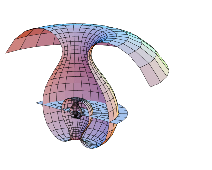
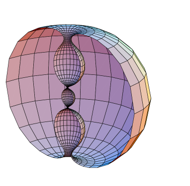
Figure 17. A discrete minimal surface of revolution in $\mathbb{H}^{3}$ (in two copies of the upper-half space model – one above the central plane, and one below), and a discrete minimal surface of revolution in $\mathbb{S}^{3}$ (where $\mathbb{S}^{3}$ has been stereographically projected to $\mathbb{R}^{3}$).

9.10. Discrete CMC surfaces of revolution

We take $Q$ as in (8.3). Let us first make the following assumption about the vertices of the discrete surface, implying we have a discrete surface of revolution:

$$\text{Assumption 1:}\;\;\mathfrak{f}_{(m,n)}=r_{m}(c_{n}i+s_{n}j)+h_{m}k\;,$$

where $c_{n}=\cos(2\pi\theta_{n}/N)$, $s_{n}=\sin(2\pi\theta_{n}/N)$ and $r_{m},h_{m}\in\mathbb{R}$, with $N$ a natural number and $\theta_{n}\in\mathbb{R}$.

The cross ratio for the quadrilateral with vertices coming from $(m,n)$, $(m+1,n)$, $(m+1,n+1)$ and $(m,n+1)$ is

$$q=q_{m,n}=\frac{-dh_{m,m+1}^{2}-dr_{m,m+1}^{2}}{4r_{m}r_{m+1}\sin^{2}(\pi d\theta_{n,n+1}/N)}\;,$$

where $dr_{m,m+1}=r_{m+1}-r_{m}$, $dh_{m,m+1}=h_{m+1}-h_{m}$ and $d\theta_{n,n+1}=\theta_{n+1}-\theta_{n}$. So we can take

$$a_{(m,n),(m+1,n)}=-\alpha\frac{dh_{m,m+1}^{2}+dr_{m,m+1}^{2}}{r_{m}r_{m+1}}\;,$$

$$a_{(m,n),(m,n+1)}=4\alpha\sin^{2}(\pi d\theta_{n,n+1}/N)$$

for any choice of $\alpha\in\mathbb{R}\setminus\{0\}$. Because $d\mathfrak{f}_{pq}^{*}d\mathfrak{f}_{pq}=a_{pq}$, we have

$$d\mathfrak{f}^{*}_{pq}=\pm\frac{\alpha}{r_{p}r_{q}}d\mathfrak{f}_{pq}\;,$$

where ”$+$” is used for $m$-edges and ”$-$” for $n$-edges. The $m$-edges are those between $\mathfrak{f}_{(m,n)}$ and $\mathfrak{f}_{(m+1,n)}$, and the $n$-edges are those between $\mathfrak{f}_{(m,n)}$ and $\mathfrak{f}_{(m,n+1)}$.

We then have

$$\tau_{pq}=\pm\frac{\alpha}{r_{p}r_{q}}\begin{pmatrix}\mathfrak{f}_{p}d\mathfrak{f}_{pq}&-\mathfrak{f}_{p}d\mathfrak{f}_{pq}\mathfrak{f}_{q}\\ d\mathfrak{f}_{pq}&-d\mathfrak{f}_{pq}\mathfrak{f}_{q}\end{pmatrix}\;.$$

Now assume $\mathfrak{f}$ is a discrete CMC surface, that is:

$$\text{Assumption 2:}\;\;\mathfrak{f}\;\text{has a linear conserved quantity}\;\;Q+\lambda Z\;.$$

Then, by Corollary 9.37, we have

$$Z_{p}=\begin{pmatrix}n_{p}+H_{p}\mathfrak{f}_{p}&-\mathfrak{f}_{p}n_{p}-n_{p}\mathfrak{f}_{p}-H_{p}\mathfrak{f}_{p}^{2}\\ H_{p}&-n_{p}-H_{p}\mathfrak{f}_{p}\end{pmatrix}\;.$$

Definition 9.45.

We say that the surface of revolution $\mathfrak{f}_{m,n}$ has a constant hyperbolic speed parametrization if the cross ratio $q_{m,n}$ is a constant (i.e. indep of $m$ and $n$).

We now restrict to the case in the above definition:

$$\text{Assumption 3:}\;\;\mathfrak{f}\;\text{is a constant hyperbolic speed parametrization}\;.$$

This third assumption is not so essential for the arguments here, but we include it as it is geometrically natural.

The last two equations in Lemma 9.31 now give the four equations

$$d\mathfrak{f}_{pq}n_{q}+n_{p}d\mathfrak{f}_{pq}=0\;,$$

$$H_{q}=H_{p}+(\kappa\mathfrak{f}_{p}d\mathfrak{f}_{pq}+\kappa d\mathfrak{f}_{pq}\mathfrak{f}_{q})\cdot\frac{\pm\alpha}{r_{p}r_{q}}\;,$$

$$n_{q}+H_{q}\mathfrak{f}_{q}=n_{p}+H_{p}\mathfrak{f}_{p}+(d\mathfrak{f}_{pq}+\kappa\mathfrak{f}_{p}d\mathfrak{f}_{pq}\mathfrak{f}_{q})\cdot\frac{\pm\alpha}{r_{p}r_{q}}\;,$$

$$\mathfrak{f}_{q}n_{q}+n_{q}\mathfrak{f}_{q}+H_{q}\mathfrak{f}_{q}^{2}=\mathfrak{f}_{p}n_{p}+n_{p}\mathfrak{f}_{p}+H_{p}\mathfrak{f}_{p}^{2}+(d\mathfrak{f}_{pq}\mathfrak{f}_{q}+\mathfrak{f}_{p}d\mathfrak{f}_{pq})\cdot\frac{\pm\alpha}{r_{p}r_{q}}\;.$$

We now assume that $n_{p}$, and hence the conserved quantity as well, has the same rotation symmetry as the surface itself:

$$\text{Assumption 4:}\;\;n_{p}=\rho_{p}(c_{n}i+s_{n}j)+\eta_{p}k\;\;\text{and}\;\;\rho_{p},\eta_{p}\in\mathbb{R}\;\text{depend only on}\;m\;.$$

The fact that $||Z_{p}||^{2}$ is constant implies $|n_{p}|^{2}$ is constant, and thus $\rho_{p}^{2}+\eta_{p}^{2}$ is also constant. We have the following further facts:

$$\mathfrak{f}_{p}n_{p}+n_{p}\mathfrak{f}_{p}+H_{p}\mathfrak{f}_{p}^{2}=-2(r_{p}\rho_{p}+h_{p}\eta_{p})-H_{p}(r_{p}^{2}+h_{p}^{2})\;,$$

and when $p=(m,n)$ and $q=(m,n+1)$, we have

$$\mathfrak{f}_{p}d\mathfrak{f}_{pq}+d\mathfrak{f}_{pq}\mathfrak{f}_{q}=0\;,\;\;\;d\mathfrak{f}_{pq}+\kappa\mathfrak{f}_{p}d\mathfrak{f}_{pq}\mathfrak{f}_{q}=r_{p}(1+\kappa(r_{p}^{2}+h_{p}^{2}))(dc_{n,n+1}i+ds_{n,n+1}j)$$

for $dc_{n,n+1}=c_{n+1}-c_{n}$ and $ds_{n,n+1}=s_{n+1}-s_{n}$. When $p=(m,n)$ and $q=(m+1,n)$, we have

$$\mathfrak{f}_{p}d\mathfrak{f}_{pq}+d\mathfrak{f}_{pq}\mathfrak{f}_{q}=r_{m}^{2}+h_{m}^{2}-r_{m+1}^{2}-h_{m+1}^{2}$$

and

$$d\mathfrak{f}_{pq}+\kappa\mathfrak{f}_{p}d\mathfrak{f}_{pq}\mathfrak{f}_{q}=(dr_{m,m+1}+\kappa(r_{m+1}(r_{m}^{2}+h_{m}^{2})-r_{m}(r_{m+1}^{2}+h_{m+1}^{2})))(c_{n}i+s_{n}j)+$$

$$+(dh_{m,m+1}+\kappa(h_{m+1}(r_{m}^{2}+h_{m}^{2})-h_{m}(r_{m+1}^{2}+h_{m+1}^{2})))k\;.$$

Now the full list of equations becomes:

1. $\rho_{m}^{2}+\eta_{m}^{2}$ is constant, where we now denote $\rho_{p}$ and $\eta_{p}$ by $\rho_{m}$ and $\eta_{m}$, respectively,

2. $H_{p}$ depends only on $m$,

3. $\rho_{m}+H_{m}r_{m}=-\alpha r_{m}^{-1}(1+\kappa(r_{m}^{2}+h_{m}^{2}))$,

4. $(\rho_{m+1}+\rho_{m})dr_{m,m+1}+(\eta_{m+1}+\eta_{m})dh_{m,m+1}=0$,

5. $dr_{m,m+1}d\eta_{m,m+1}-dh_{m,m+1}d\rho_{m,m+1}=0$,

6. $H_{m+1}-H_{m}=\alpha\kappa r_{m}^{-1}r_{m+1}^{-1}(r_{m}^{2}+h_{m}^{2}-r_{m+1}^{2}-h_{m+1}^{2})$,

7. $d\rho_{m,m+1}+H_{m+1}r_{m+1}-H_{m}r_{m}=\alpha r_{m}^{-1}r_{m+1}^{-1}(dr_{m,m+1}+\kappa(r_{m+1}(r_{m}^{2}+h_{m}^{2})-r_{m}(r_{m+1}^{2}+h_{m+1}^{2})))$,

8. $d\eta_{m,m+1}+H_{m+1}h_{m+1}-H_{m}h_{m}=\alpha r_{m}^{-1}r_{m+1}^{-1}(dh_{m,m+1}+\kappa(h_{m+1}(r_{m}^{2}+h_{m}^{2})-h_{m}(r_{m+1}^{2}+h_{m+1}^{2})))$,

9. $2(r_{m}\rho_{m}+h_{m}\eta_{m}-r_{m+1}\rho_{m+1}-h_{m+1}\eta_{m+1})+H_{m}(r_{m}^{2}+h_{m}^{2})-H_{m+1}(r_{m+1}^{2}+h_{m+1}^{2})=\alpha r_{m}^{-1}r_{m+1}^{-1}(r_{m}^{2}+h_{m}^{2}-r_{m+1}^{2}-h_{m+1}^{2})$.

The first condition above should follow from the other equations, and we can just assume the second condition. We then have the system

(9.41) $$P\cdot\begin{pmatrix}H_{m}\\ H_{m+1}\\ \eta_{m}\\ \eta_{m+1}\\ \rho_{m}\\ \rho_{m+1}\\ H_{\kappa}\\ 1\end{pmatrix}=\begin{pmatrix}0\\ 0\\ 0\\ 0\\ 0\\ 0\\ 0\\ 0\end{pmatrix}\;,$$

$$P=\begin{pmatrix}r_{m}^{2}&0&0&0&r_{m}&0&0&A\\ 0&r_{m+1}^{2}&0&0&0&r_{m+1}&0&B\\ 0&0&dh_{m,m+1}&dh_{m,m+1}&dr_{m,m+1}&dr_{m,m+1}&0&0\\ 0&0&-dr_{m,m+1}&dr_{m,m+1}&dh_{m,m+1}&-dh_{m,m+1}&0&0\\ -1&1&0&0&0&0&0&\kappa C\\ -r_{m}&r_{m+1}&0&0&-1&1&0&D\\ -h_{m}&h_{m+1}&-1&1&0&0&0&E\\ r_{m}^{2}+h_{m}^{2}&-r_{m+1}^{2}-h_{m+1}^{2}&2h_{m}&-2h_{m+1}&2r_{m}&-2r_{m+1}&0&C\end{pmatrix}\;,$$

where

$$A=\alpha(1+\kappa(r_{m}^{2}+h_{m}^{2}))\;,$$

$$B=\alpha(1+\kappa(r_{m+1}^{2}+h_{m+1}^{2}))\;,$$

$$C=\alpha r_{m}^{-1}r_{m+1}^{-1}(r_{m+1}^{2}+h_{m+1}^{2}-r_{m}^{2}-h_{m}^{2})\;,$$

$$D=-\alpha r_{m}^{-1}r_{m+1}^{-1}(dr_{m,m+1}+\kappa(r_{m+1}(r_{m}^{2}+h_{m}^{2})-r_{m}(r_{m+1}^{2}+h_{m+1}^{2})))\;,$$

$$E=-\alpha r_{m}^{-1}r_{m+1}^{-1}(dh_{m,m+1}+\kappa(h_{m+1}(r_{m}^{2}+h_{m}^{2})-h_{m}(r_{m+1}^{2}+h_{m+1}^{2})))\;.$$

The fifth and eighth rows of the product on the left-hand side of (9.41) being zero implies that

$$H_{m+1}-H_{m}=2\kappa(r_{m}\rho_{m}+h_{m}\eta_{m}-r_{m+1}\rho_{m+1}-h_{m+1}\eta_{m+1})+$$

$$+H_{m}(r_{m}^{2}+h_{m}^{2})\kappa-H_{m+1}(r_{m+1}^{2}+h_{m+1}^{2})\kappa\;,$$

and so

$$2H_{\kappa}:=H_{m+1}(1+\kappa(r_{m+1}^{2}+h_{m+1}^{2}))+2\kappa(r_{m+1}\rho_{m+1}+h_{m+1}\eta_{m+1})=$$

$$=H_{m}(1+\kappa(r_{m}^{2}+h_{m}^{2}))+2\kappa(r_{m}\rho_{m}+h_{m}\eta_{m})$$

is constant.

We can then choose the constant $\alpha$ so that $\eta_{m}^{2}+\rho_{m}^{2}=1$, and then start with some initial conditions and propagate through values of $m$ via (9.41) to produce the vertex data for a discrete CMC surface of revolution.

Figure 18. Discrete profile curves for discrete CMC surfaces of revolution. The meanings of these graphics are explained in Example 9.46.

Example 9.46.

In Figure 18, we show discrete CMC surfaces of revolution. The first two curves are profile curves for discrete nonminimal CMC surfaces of revolution in $\mathbb{R}^{3}$, the first being unduloidal and the second nodoidal. (For each of these two curves, the axis of rotation producing the surface is a vertical line drawn to the left of the curve, and is not shown in the figure.) The third picture shows the profile curve for a discrete CMC surface of revolution in $\mathbb{S}^{3}$, where $\mathbb{S}^{3}$ is stereographically projected to $\mathbb{R}^{3}$, and the circle shown is a geodesic of $\mathbb{S}^{3}$ that is also the axis of the surface – and furthermore, this example has a periodicity that causes it to close on itself and form a torus. Half of this surface in $\mathbb{S}^{3}$ is shown on the right-hand side of Figure 17 as well, under a different stereographic projection to $\mathbb{R}^{3}$. The final two pictures in Figure 18 show profile curves for discrete CMC surfaces of revolution in $\mathbb{H}^{3}$. These surfaces, with $H>1$ and $H=1$ respectively, are shown in the Poincare model, and the first is unduloidal while the second looks similar to a smooth embedded catenoid cousin. (For these two curves, the corresponding axis of revolution is the vertical line between the uppermost and lowermost points of the circle shown, and this circle lies in the boundary sphere at infinity of $\mathbb{H}^{3}$.) Also, on the left-hand side of Figure 17, we see a minimal surface that lies in both copies of $M_{-1}=\mathbb{H}^{3}\cup\mathbb{H}^{3}$, and the horizontal plane shown there is the virtual boundary at infinity of two copies of the halfspace model for $\mathbb{H}^{3}$. This example was first known in [27], because the notion of discrete CMC for this case was not defined before then.

10. Discrete spacelike CMC surfaces in $\mathbb{R}^{2,1}$

In Chapter 7, we looked at smooth maximal surfaces in Minkowski $3$-space. In this chapter, we consider one way to define discrete versions of them, and more generally, to define discrete spacelike CMC surfaces in $\mathbb{R}^{2,1}$. We start by reviewing the smooth case.

10.1. Smooth CMC surfaces in $\mathbb{R}^{3}$ and $\mathbb{R}^{2,1}$, without quaternions

Consider a smooth surface

$$x(u,v)=(x_{1}(u,v),x_{2}(u,v),x_{3}(u,v))$$

in $\mathbb{R}^{3}$ or $\mathbb{R}^{2,1}$, with unit normal $n$. Suppose the surface is spacelike, in the case of $\mathbb{R}^{2,1}$. Also, suppose that the coordinates $u,v$ are isothermic. Conformality implies the first fundamental form is

$$I=\begin{pmatrix}E&0\\ 0&E\end{pmatrix}$$

with $E=\langle x_{u},x_{u}\rangle$, where $\langle\cdot,\cdot\rangle$ denotes the inner product associated with $\mathbb{R}^{3}$ or $\mathbb{R}^{2,1}$. Then the second fundamental form is

$$II=\begin{pmatrix}\langle n,x_{uu}\rangle&\langle n,x_{vu}\rangle\\ \langle n,x_{uv}\rangle&\langle n,x_{vv}\rangle\end{pmatrix}=\begin{pmatrix}b_{11}&b_{12}\\ b_{21}&b_{22}\end{pmatrix}\;,$$

and having isothermic coordinates implies $n_{u}=-k_{1}x_{u}$ and $n_{v}=-k_{2}x_{v}$, where $k_{1}$ and $k_{2}$ are the principal curvatures, and so

$$II=\begin{pmatrix}k_{1}E&0\\ 0&k_{2}E\end{pmatrix}\;.$$

The Hopf differential function is, with $z=u+iv$,

$$\hat{Q}=\langle n,x_{zz}\rangle=\frac{1}{4}\langle n,x_{uu}-x_{vv}-2ix_{uv}\rangle=\frac{1}{4}\langle n,x_{uu}-x_{vv}\rangle$$

$$=\frac{1}{4}(b_{11}-b_{22})=\frac{E}{4}(k_{1}-k_{2})\;.$$

If the mean curvature $H$ is constant, then Corollary 8.22 and the second equation in (7.2) imply $\hat{Q}_{\bar{z}}=0$, so $\hat{Q}=(E/4)(k_{1}-k_{2})\in\mathbb{R}$ is constant.

Lemma 10.1.

If $x$ is isothermic in $\mathbb{R}^{3}$ or $\mathbb{R}^{2,1}$ with isothermic coordinates $u,v$, then $x^{*}$ exists, solving $dx^{*}=-\frac{x_{u}}{E}du+\frac{x_{v}}{E}dv$.

Proof.

This was already proven in the case of $\mathbb{R}^{3}$ in Lemma 8.15, so let us be brief here: We want to show ”$d^{2}x^{*}=0$”, i.e.

$$d(-\frac{x_{u}}{E}du+\frac{x_{v}}{E}dv)=\;0,$$

i.e. $2x_{uv}E-x_{u}E_{v}-x_{v}E_{u}=0$. We can see this by noting that $b_{12}=0$ implies $x_{uv}=Ax_{u}+Bx_{v}$ for some reals $A$ and $B$, and that $\langle x_{u},x_{v}\rangle=0$. ∎

The $x^{*}$ in Lemma 10.1 is the same as the $x^{*}$ in Definition 8.17, but scaled by a factor of $1/4$. This is a non-essential change.

Proposition 10.2.

Let $x$ be an isothermic immersion in $\mathbb{R}^{3}$ or $\mathbb{R}^{2,1}$, with $x^{*}$ as in the previous lemma. Then $x$ is CMC $H$ if and only if $dx^{*}=h(Hdx+dn)$ for some constant $h$.

Proof.

Let us again be brief, because the $\mathbb{R}^{3}$ case was already dealt with in Remark 8.19:

$$-\frac{x_{u}}{E}du+\frac{x_{v}}{E}dv=h(Hdx+dn)\;,\;\;\;h\;\,\text{constant}$$

is equivalent to

$$k_{1}+k_{2}=2H\;,\;\;\text{and}\;\;h=2E^{-1}(k_{1}-k_{2})^{-1}\;\text{is constant}\;.$$

The first of these is clearly true, and $h$ is constant if and only if the Hopf differential function $\hat{Q}$ is constant, which is true if and only if $x$ is CMC. ∎

Corollary 10.3.

An isothermic immersion $x$ in $\mathbb{R}^{3}$ or $\mathbb{R}^{2,1}$ is CMC if and only if

$$-\frac{x_{u}}{E}du+\frac{x_{v}}{E}dv=h(Hdx+dn)$$

for some real constants $h$ and $H$.

10.2. Discrete isothermic CMC surfaces in $\mathbb{R}^{3}$, without quaternions

Let $\mathfrak{f}$ be a discrete isothermic surface in $\text{Im}H\approx\mathbb{R}^{3}$ as in Chapter 9, with cross ratio factorizing function $a_{pq}$. Starting with the equation

$$d\mathfrak{f}_{pq}^{*}=a_{pq}\frac{-d\mathfrak{f}_{pq}}{|d\mathfrak{f}_{pq}|^{2}}$$

for the Christoffel transformation, we have the following lemma, which follows from Corollary 9.36:

Lemma 10.4.

A discrete isothermic surface $\mathfrak{f}$ in $\mathbb{R}^{3}$ is CMC if and only if there exist constants $h,H\in\mathbb{R}$ and $n_{p}$ with $|n_{p}|^{2}=1$ and $d\mathfrak{f}_{pq}n_{q}+n_{p}d\mathfrak{f}_{pq}=0$ so that

$$h(dn_{pq}+Hd\mathfrak{f}_{pq})=\frac{-a_{pq}d\mathfrak{f}_{pq}}{|d\mathfrak{f}_{pq}|^{2}}\;.$$

However, $d\mathfrak{f}_{pq}n_{q}+n_{p}d\mathfrak{f}_{pq}=0$ is still a quaternionic equation. But this equation is equivalent to the pair of equations $d\mathfrak{f}_{pq}\wedge n_{q}+n_{p}\wedge d\mathfrak{f}_{pq}=0$ and $\langle d\mathfrak{f}_{pq},n_{p}+n_{q}\rangle_{\mathbb{R}^{3}}=0$. Then we can restate the previous lemma, without any use of quaternions, as:

Theorem 10.5.

A discrete isothermic surface $\mathfrak{f}$ in $\mathbb{R}^{3}$ is CMC if and only if there exist constants $h,H\in\mathbb{R}$ and vectors $n_{p}$ so that

• $|n_{p}|^{2}=1$,

• $d\mathfrak{f}_{pq}\wedge n_{q}+n_{p}\wedge d\mathfrak{f}_{pq}=0$,

• $\langle d\mathfrak{f}_{pq},n_{p}+n_{q}\rangle_{\mathbb{R}^{3}}=0$, and

• $h(dn_{pq}+Hd\mathfrak{f}_{pq})=\frac{-a_{pq}d\mathfrak{f}_{pq}}{|d\mathfrak{f}_{pq}|^{2}}$.

Not all four items in the above theorem are independent of each other. For example, the second item follows from the fourth item, because the second item is just telling us that $d\mathfrak{f}_{pq}$ is parallel to $dn_{pq}$.

10.3. Discrete CMC surfaces in $\mathbb{R}^{2,1}$

We now propose possible definitions for discrete isothermic surfaces and discrete spacelike CMC surfaces in $\mathbb{R}^{2,1}$.

Let $\mathfrak{f}$ be a map from a domain in $\mathbb{Z}^{2}$ to $\mathbb{R}^{2,1}$. Let $p=(m,n)$, $q=(m+1,n)$, $r=(m+1,n+1)$ and $s=(m,n+1)$ be four vertices in the domain of $\mathfrak{f}$, for some $m,n\in\mathbb{Z}$. Let $\mathfrak{f}_{p}$, $\mathfrak{f}_{q}$, $\mathfrak{f}_{r}$ and $\mathfrak{f}_{s}$ be the images of $p$, $q$, $r$ and $s$ under $\mathfrak{f}$.

To define the cross ratio factorizing function $a_{pq}$ in the case of $\mathbb{R}^{2,1}$, we need to define some analogue of the cross ratio, call it $q=q_{pqrs}$. Then we can define the $a_{pq}$ in the usual way.

We now consider how to define the cross ratio on quadrilaterals. We could consider quadrilaterals in spacelike planes, without rotating those planes to horizontal. However, in the argument below we choose to rotate the planes to horizontal, so that the metric will be exactly the Euclidean metric that is so familiar to us.

We assume that the points $\mathfrak{f}_{p},\mathfrak{f}_{q},\mathfrak{f}_{r},\mathfrak{f}_{s}$ lie in a ”circle” in a spacelike plane of $\mathbb{R}^{2,1}$. In general, such a circle is

$$\left\{\left.\begin{pmatrix}\cos\beta&\sin\beta&0\\ -\sin\beta&\cos\beta&0\\ 0&0&1\end{pmatrix}\begin{pmatrix}\cosh\gamma&0&\sinh\gamma\\ 0&1&0\\ \sinh\gamma&0&\cosh\gamma\end{pmatrix}\begin{pmatrix}\rho\cos\theta\\ \rho\sin\theta\\ 0\end{pmatrix}+\begin{pmatrix}x_{0}\\ y_{0}\\ z_{0}\end{pmatrix}\,\right|\,\theta\in[0,2\pi)\right\}\;,$$

where $x_{0},y_{0},z_{0},\rho,\gamma,\beta$ are all real constants. By a rigid motion of $\mathbb{R}^{2,1}$, we can move this circle to the horizontal circle

$$\{(\rho\cos\theta,\rho\sin\theta,0)\,|\,\theta\in[0,2\pi)\}\;.$$

Then the points $\mathfrak{f}_{p},\mathfrak{f}_{q},\mathfrak{f}_{r},\mathfrak{f}_{s}$ are moved to points $(\rho\cos\theta_{*},\rho\sin\theta_{*},0)$ for $*=p,q,r,s$, respectively.

Then we can compute the cross ratio in the usual way for the space $\mathbb{R}^{3}$ (that is, we can replace the metric for $\mathbb{R}^{2,1}$ with the metric for $\mathbb{R}^{3}$ and then compute the cross ratio, which is allowed because the circle is now horizontal in $\mathbb{R}^{2,1}$):

$$q_{pqrs}=\sin(\frac{\theta_{p}-\theta_{q}}{2})\csc(\frac{\theta_{q}-\theta_{r}}{2})\sin(\frac{\theta_{r}-\theta_{s}}{2})\csc(\frac{\theta_{s}-\theta_{p}}{2})\;.$$

Remark 10.6.

This $q_{pqrs}$ is invariant under isometries of $\mathbb{R}^{2,1}$ (by definition), but is not Möbius invariant (unlike the case of $\mathbb{R}^{3}$).

Once the $q_{qprs}$ are defined, then the $a_{pq}$ can be defined by

$$q_{pqrs}=a_{pq}/a_{ps}\;,$$

and then we could use the same equations as for the $\mathbb{R}^{3}$ case, that is, the equations in Definition 9.5, to determine when the surface is discrete isothermic, with spacelike quadrilaterals.

Then, after restricting to discrete isothermic surfaces, we could define discrete spacelike CMC surfaces in $\mathbb{R}^{2,1}$ by imitating the equations from the case of discrete CMC surfaces in $\mathbb{R}^{3}$, as found in Theorem 10.5. This is justified by looking at smooth CMC surfaces in $\mathbb{R}^{3}$ and $\mathbb{R}^{2,1}$, which have exactly the same equations – only the ambient metric changes, see Corollary 10.3.

So the equations we want for defining a discrete spacelike CMC surface in $\mathbb{R}^{2,1}$ are as follows: there exist $h,H\in\mathbb{R}$ and normals $n_{p}$ so that

1. $\langle n_{p},n_{p}\rangle_{\mathbb{R}^{2,1}}=-1$,

2. $d\mathfrak{f}_{pq}\wedge n_{q}+n_{p}\wedge d\mathfrak{f}_{pq}=0$,

3. $\langle d\mathfrak{f}_{pq},n_{p}+n_{q}\rangle_{\mathbb{R}^{2,1}}=0$, and

4. $h(dn_{pq}+Hd\mathfrak{f}_{pq})=\frac{-a_{pq}d\mathfrak{f}_{pq}}{|d\mathfrak{f}_{pq}|^{2}}$,

where here $\langle\cdot,\cdot\rangle_{\mathbb{R}^{2,1}}$ represents the $\mathbb{R}^{2,1}$ inner product, and $\wedge$ is the $\mathbb{R}^{2,1}$ cross product, and $|\cdot|$ is the $\mathbb{R}^{2,1}$ norm.

11. Polynomial conserved quantities and Darboux transforms

11.1. Polynomial conserved quantities

Equation (9.33) can be extended to define discrete isothermic surfaces $\mathfrak{f}$ with polynomial conserved quantities, as follows:

Definition 11.1.

$$P=Q+\lambda P_{1}+\lambda^{2}P_{2}+...+\lambda^{n-1}P_{n-1}+\lambda^{n}Z$$

is a polynomial conserved quantity if

(11.1) $$(I+\lambda\tau_{pq})P_{q}=P_{p}(I+\lambda\tau_{pq})\;,$$

where $Q$, $Z$ and the $P_{j}$ are maps from the lattice domain to $\mathbb{R}^{4,1}$.

We sometimes write $Z$ as $P_{n}$ as well. If such a polynomial conserved quantity exists, we say that $\mathfrak{f}$ is a special surface of type $n$, and the above Equation (11.1) is equivalent to

(11.2) $$T^{\lambda}_{p}P_{p}(T^{\lambda}_{p})^{-1}$$

being constant with respect to the vertices $p$.

Equation (11.1) can be restated as $\Gamma_{pq}^{\lambda}\cdot P_{q}=P_{p}$, i.e. $P$ is a parallel section, i.e. $P$ is conserved by the connection $\Gamma_{pq}^{\lambda}$, so we can call it a ”conserved quantity”.

11.2. Polynomial conserved quantities for smooth surfaces

Before further exploring discrete surfaces with polynomial conserved quantities, let us consider the case of smooth surfaces. Definition 8.23 and Equation (8.12) can be extended to define smooth surfaces with polynomial conserved quantities

$$P=Q+\lambda P_{1}+\lambda^{2}P_{2}+...+\lambda^{n-1}P_{n-1}+\lambda^{n}Z\;,$$

where $Q$, $Z$ and the $P_{j}$ are maps from the domain of definition of $x=x(u,v)$ to $\mathbb{R}^{4,1}$, as follows:

Definition 11.2.

$P$ is a polynomial conserved quantity of type $n$ if

(11.3) $$dP=\lambda P\tau-\lambda\tau P\;.$$

We now state a result about the polynomial conserved quantities of Darboux transforms of smooth surfaces (recall that Darboux transformations were defined in Definition 8.49):

Lemma 11.3.

If the initial isothermic surface $x=x(u,v)$ has a polynomial conserved quantity of order $n$, then any Darboux transform $\hat{x}=\hat{x}(u,v)$ has a polynomial conserved quantity of order at most $n+1$.

Proof.

Let $X$ be a lift of the initial surface $x$ with Calapso transformation $T$ and polynomial conserved quantity $P$ of order $n$. Then $TPT^{-1}$ is constant. Let $\hat{X}$ be a lift of the Darboux transform $\hat{x}$ of $x$, i.e. $T\hat{X}T^{-1}$ is constant in $PL^{4}$ for some particular choice of $\lambda$, and let us refer to that choice of $\lambda$ as $\lambda=\mu$. (From now on we take $\mu$ to be that fixed value, and $\lambda$ will denote a free real parameter.) We define

$$A=I-\frac{\lambda}{\mu}\frac{X\hat{X}}{X\hat{X}+\hat{X}X}$$

(since $X\hat{X}+\hat{X}X$ is a scalar multiple of the identity, we regard it as a scalar in the denominator here), and we can check that

$$A^{-1}=\frac{1}{(\mu-\lambda)(X\hat{X}+\hat{X}X)}(\mu X\hat{X}+(\mu-\lambda)\hat{X}X)\;,$$

which follows immediately from the property $X^{2}=\hat{X}^{2}=0$.

Since we are free to rescale $X$ and $\hat{X}$, let us rescale them so that

$$X=\begin{pmatrix}x&-x^{2}\\ 1&-x\end{pmatrix}\;,\;\;\;\hat{X}=\frac{1}{\delta^{2}}\begin{pmatrix}\hat{x}&-\hat{x}^{2}\\ 1&-\hat{x}\end{pmatrix}\;,$$

where $\delta:=\hat{x}-x$. Then

$$X\hat{X}=\frac{1}{\delta^{2}}\begin{pmatrix}x\delta&-x\delta\hat{x}\\ \delta&-\delta\hat{x}\end{pmatrix}\;,\;\;\;\hat{X}X=\frac{1}{\delta^{2}}\begin{pmatrix}-\hat{x}\delta&\hat{x}\delta x\\ -\delta&\delta x\end{pmatrix}\;,$$

and also

$$X\hat{X}+\hat{X}X=-I\;,\;\;\;x\delta\hat{x}=\hat{x}\delta x\;.$$

We also have that the logarithmic derivatives $\tau$ and $\hat{\tau}$ of Calapso transformations of $x$ and $\hat{x}$ satisfy

$$\tau(\partial_{u})=\begin{pmatrix}xx_{u}^{-1}&-xx_{u}^{-1}x\\ x_{u}^{-1}&-x_{u}^{-1}x\end{pmatrix}\;,\;\;\;\tau(\partial_{v})=-\begin{pmatrix}xx_{v}^{-1}&-xx_{v}^{-1}x\\ x_{v}^{-1}&-x_{v}^{-1}x\end{pmatrix}\;,$$

$$\hat{\tau}(\partial_{u})=\begin{pmatrix}\hat{x}\hat{x}_{u}^{-1}&-\hat{x}\hat{x}_{u}^{-1}\hat{x}\\ \hat{x}_{u}^{-1}&-\hat{x}_{u}^{-1}\hat{x}\end{pmatrix}\;,\;\;\;\hat{\tau}(\partial_{v})=-\begin{pmatrix}\hat{x}\hat{x}_{v}^{-1}&-\hat{x}\hat{x}_{v}^{-1}\hat{x}\\ \hat{x}_{v}^{-1}&-\hat{x}_{v}^{-1}\hat{x}\end{pmatrix}\;.$$

Furthermore, by Equation (8.24), we have

(11.4) $$\hat{x}_{u}=\mu\delta x_{u}^{-1}\delta\;,\;\;\;\hat{x}_{v}=-\mu\delta x_{v}^{-1}\delta\;.$$

Next we should show that $d(TA)=TA\cdot\lambda\hat{\tau}$, so $\hat{T}=TA$ solves $\hat{T}^{-1}d\hat{T}=\lambda\hat{\tau}$. That is, we wish to show that

$$A^{-1}\lambda\tau(\partial_{u})A+A^{-1}dA-\lambda\hat{\tau}(\partial_{u})=$$

$$\frac{\mu\lambda}{\mu-\lambda}\begin{pmatrix}xx_{u}^{-1}&-xx_{u}^{-1}x\\ x_{u}^{-1}&-x_{u}^{-1}x\end{pmatrix}-\lambda\begin{pmatrix}\hat{x}\hat{x}_{u}^{-1}&-\hat{x}\hat{x}_{u}^{-1}\hat{x}\\ \hat{x}_{u}^{-1}&-\hat{x}_{u}^{-1}\hat{x}\end{pmatrix}-\frac{\lambda(\delta\delta_{u}+\delta_{u}\delta)}{(\mu-\lambda)\delta^{4}}\begin{pmatrix}x\delta&-x\delta\hat{x}\\ \delta&-\delta\hat{x}\end{pmatrix}+$$

$$\frac{\lambda}{(\mu-\lambda)\delta^{2}}\begin{pmatrix}x_{u}\delta+x\delta_{u}&-x_{u}\delta\hat{x}-x\delta_{u}\hat{x}-x\delta\hat{x}_{u}\\ \delta_{u}&-\delta_{u}\hat{x}-\delta\hat{x}_{u}\end{pmatrix}+\frac{\lambda^{2}}{\mu(\mu-\lambda)\delta^{4}}\begin{pmatrix}-\hat{x}\delta x_{u}\delta&\hat{x}\delta x_{u}\delta\hat{x}\\ -\delta x_{u}\delta&\delta x_{u}\delta\hat{x}\end{pmatrix}$$

is zero, and also $A^{-1}\lambda\tau(\partial_{v})A+A^{-1}dA-\lambda\hat{\tau}(\partial_{v})=0$, and this follows from the first equation in (11.4).

Then we define

$$\hat{P}=\mu(\mu-\lambda)A^{-1}PA\;,$$

and we can show that $\hat{T}\hat{P}\hat{T}^{-1}$ is constant, as follows: $d(\hat{T}\hat{P}\hat{T}^{-1})=\mu(\mu-\lambda)d(TA\cdot A^{-1}PA\cdot A^{-1}T^{-1})=\mu(\mu-\lambda)d(TPT^{-1})=0$.

It is now clear that $\hat{P}$ is a polynomial conserved quantity of degree at most $n+2$. To show that the degree is actually at most $n+1$, it suffices to show that $P_{n}$ is perpendicular to $X$, and so $XP_{n}X=0$. We omit an argument for this, but note that the analogous argument for the case of discrete surfaces can be found in detail below. ∎

Remark 11.4.

The Darboux transform in Lemma 11.3 is a Baecklund transform exactly when it is of type at most $n$. See Remarks 8.52 and 8.53. See also Definition 11.28 and Lemma 11.30 (discrete case).

For an isothermic surface with a polynomial conserved quantity of order $n$, we define a complementary surface as follows: take a value $\lambda_{0}$ of $\lambda$ so that

$$||P(\lambda_{0})||^{2}=||Q+\lambda_{0}P_{1}+\lambda^{2}_{0}P_{2}+...+\lambda^{n-1}_{0}P_{n-1}+\lambda^{n}_{0}Z||^{2}=0$$

and define the complementary surface to be $P(\lambda_{0})$. This will be a Baecklund transformation, so will be of type at most $n$. We say more about this in Section 11.6.

Complementary surfaces can be of type $n$. But if a Baecklund transform is of type $n-1$ (Darboux transforms must be of type at least $n-1$, as seen in Lemma 11.22), then it must be a complementary surface, by Lemma 4.10 of [27]. Examples of type $n-1$ Baecklund transforms can come from CMC $1$ surfaces in $\mathbb{H}^{3}$ and minimal surfaces in $\mathbb{R}^{3}$. In fact, we have the following lemma:

Lemma 11.5.

In the case $n=1$ (i.e. CMC surfaces), CMC $\pm\sqrt{-\kappa}$ surfaces in $M_{\kappa}$ are the only cases where a type $n-1=0$ Baecklund transform can exist. In particular, if such a Baecklund transform exists, then $\kappa\leq 0$.

Proof.

When the linear conserved quantity is normalized, we have

$$||\lambda Z+Q||^{2}=\lambda^{2}-2H\lambda-\kappa\;,$$

and the discriminant is

$$2\sqrt{H^{2}+\kappa}\;.$$

When a type $0$ Baecklund transform exists, we have a higher order zero of $\lambda^{2}-2H\lambda-\kappa$ (by Lemma 4.10 in [27]), so $H^{2}+\kappa=0$, i.e. $H^{2}=-\kappa$. (See [27] for further details.) ∎

Remark 11.6.

Take a smooth surface and apply two Darboux transformations given by using $\lambda$ and $\mu$, respectively. Then apply a Darboux transformations to each of those, but now using $\mu$ for the case of the surface first made using $\lambda$ and using $\lambda$ for the case of the surface first made using $\mu$. By a permutability theorem, this second pair of Darboux transformations is just one single surface. Fixing one point on the original surface and looking at the other three corresponding points on the four (actually only three) transformed surfaces, one has a quadrilateral with cross ratio equal to $\lambda/\mu$. One can keep repeating this procedure to make more quadrilaterals. This will result in a discrete surface starting from a single point on the original smooth surface, and comprized of corresponding points on the transformed surfaces (one point for each transformed surface). Because the cross ratios take the form $\lambda/\mu$, this discrete surface is discrete isothermic.

11.3. Darboux transforms for discrete surfaces

The Darboux transforms of discrete surfaces have similar enveloping properties to the case of smooth surfaces. In the discrete case, the eight vertices of two corresponding quadrilaterals (one on the original surface and the corresponding one on the Darboux transform) all lie in one sphere. (This can be seen from the upcoming Lemmas 11.9 and 11.11.)

Assume $\mathfrak{f}$ is a discrete isothermic surface, and that $F$ is a lift of $\mathfrak{f}$. We have the Christoffel transformation $T^{\lambda}$ satisfying

$$T_{q}^{\lambda}=T_{p}^{\lambda}(I+\lambda\tau_{pq})\;.$$

Definition 11.7.

$\hat{F}$ gives a Darboux transform $\hat{\mathfrak{f}}$ of $\mathfrak{f}$ if

(11.5) $$T^{\mu}_{p}\hat{F}_{p}(T^{\mu}_{p})^{-1}$$

is constant in $PL^{4}$ with respect to vertices $p$, for some value $\mu$.

When the term $T^{\mu}_{p}\hat{F}_{p}(T^{\mu}_{p})^{-1}$ in Equation (11.5) is set to a constant, we have what is sometimes called Darboux’s linear system.

In this definition, $\hat{\mathfrak{f}}$ is a Darboux transformation if $T^{\mu}\hat{F}(T^{\mu})^{-1}$ is constant. Here ”constant” means in the projectivized sense. That is, there exists an $r_{pq}\in\mathbb{R}$ such that $T_{p}^{\mu}\hat{F}_{p}(T_{p}^{\mu})^{-1}=r_{pq}\cdot T_{q}^{\mu}\hat{F}_{q}(T_{q}^{\mu})^{-1}$.

Once a choice of $T$ is made, it is possible to choose $\hat{F}$ so that $r_{pq}=1$ on all edges, but then $\hat{F}$ might not be a Moutard lift.

Just like in the smooth case, where we obtained the Riccati equation (8.24), we have:

Lemma 11.8.

Definition 11.7 is equivalent to

(11.6) $$d\hat{\mathfrak{f}}_{pq}=\mu(\hat{\mathfrak{f}}-\mathfrak{f})_{p}df^{*}_{pq}(\hat{\mathfrak{f}}-\mathfrak{f})_{q}\;.$$

Proof.

We prove just one direction here. The other direction can be proven by an argument analogous to the one in the proof of Lemma 8.50, and we leave that to the reader.

$T_{q}^{\mu}\hat{F}_{q}(T_{q}^{\mu})^{-1}$ being parallel to $T_{p}^{\mu}\hat{F}_{p}(T_{p}^{\mu})^{-1}$ is equivalent to the following four equations:

$$1+\mu d\mathfrak{f}_{pq}^{*}d\mathcal{D}_{q}=r(1-\mu d\mathcal{D}_{p}d\mathfrak{f}^{*}_{pq})\;,$$

$$\hat{\mathfrak{f}}_{q}+\mu\mathfrak{f}_{p}d\mathfrak{f}_{pq}^{*}d\mathcal{D}_{q}=r(\hat{\mathfrak{f}}_{p}-\mu\hat{\mathfrak{f}}_{p}d\mathcal{D}_{p}d\mathfrak{f}^{*}_{pq})\;,$$

$$\hat{\mathfrak{f}}_{q}+\mu d\mathfrak{f}_{pq}^{*}d\mathcal{D}_{q}\hat{\mathfrak{f}}_{q}=r(\hat{\mathfrak{f}}_{p}-\mu d\mathcal{D}_{p}d\mathfrak{f}^{*}_{pq}\mathfrak{f}_{q})\;,$$

$$(\hat{\mathfrak{f}}_{q}+\mu\mathfrak{f}_{p}d\mathfrak{f}_{pq}^{*}d\mathcal{D}_{q})\hat{\mathfrak{f}}_{q}=r\hat{\mathfrak{f}}_{p}(\hat{\mathfrak{f}}_{p}-\mu d\mathcal{D}_{p}d\mathfrak{f}^{*}_{pq}\mathfrak{f}_{q})\;,$$

for some real $r$, where $d\mathcal{D}:=\hat{\mathfrak{f}}-\mathfrak{f}$. Defining $r$ by the first of the four equations, we have

$$(1-\mu d\mathcal{D}_{p}d\mathfrak{f}^{*}_{pq})(\hat{\mathfrak{f}}_{q}+\mu\mathfrak{f}_{p}d\mathfrak{f}^{*}_{pq}d\mathcal{D}_{q})\hat{\mathfrak{f}}_{q}=$$

$$(1+\mu d\mathfrak{f}^{*}_{pq}d\mathcal{D}_{q})\hat{\mathfrak{f}}_{p}(1-\mu d\mathcal{D}_{p}d\mathfrak{f}^{*}_{pq})\hat{\mathfrak{f}}_{q}=$$

$$(1-\mu d\mathcal{D}_{p}d\mathfrak{f}^{*}_{pq})\hat{\mathfrak{f}}_{p}(1+\mu d\mathfrak{f}^{*}_{pq}d\mathcal{D}_{q})\hat{\mathfrak{f}}_{q}=$$

$$(1+\mu d\mathfrak{f}^{*}_{pq}d\mathcal{D}_{q})\hat{\mathfrak{f}}_{p}(\hat{\mathfrak{f}}_{p}-\mu d\mathcal{D}_{p}d\mathfrak{f}^{*}_{pq}\mathfrak{f}_{q})\;.$$

In particular,

$$\hat{\mathfrak{f}}_{q}+\mu\mathfrak{f}_{p}d\mathfrak{f}^{*}_{pq}d\mathcal{D}_{q}=\hat{\mathfrak{f}}_{p}+\mu\hat{\mathfrak{f}}_{p}d\mathfrak{f}^{*}_{pq}d\mathcal{D}_{q}\;,$$

$$\hat{\mathfrak{f}}_{q}-\mu d\mathcal{D}_{p}d\mathfrak{f}^{*}_{pq}\hat{\mathfrak{f}}_{q}=\hat{\mathfrak{f}}_{p}-\mu d\mathcal{D}_{p}d\mathfrak{f}^{*}_{pq}\mathfrak{f}_{q}\;.$$

Summing these last two equations gives Equation (11.6). ∎

Lemma 11.9.

If $\hat{\mathfrak{f}}$ is a Darboux transform of $\mathfrak{f}$, then for adjacent $p$ and $q$, the four points $\mathfrak{f}_{p}$, $\mathfrak{f}_{q}$, $\hat{\mathfrak{f}}_{q}$ and $\hat{\mathfrak{f}}_{p}$ are concircular.

Proof.

Because $\hat{\mathfrak{f}}$ is a Darboux transformation, by (11.6) we have

$$1=\mu(\hat{\mathfrak{f}}_{p}-\mathfrak{f}_{p})d\mathfrak{f}_{pq}^{*}(\hat{\mathfrak{f}}_{q}-\mathfrak{f}_{q})(d\hat{\mathfrak{f}}_{pq})^{-1}$$

for some $\mu\in\mathbb{R}$. So

$$(\hat{\mathfrak{f}}_{p}-\mathfrak{f}_{p})(\mathfrak{f}_{q}-\mathfrak{f}_{p})^{-1}(\hat{\mathfrak{f}}_{q}-\mathfrak{f}_{q})(\hat{\mathfrak{f}}_{q}-\hat{\mathfrak{f}}_{p})^{-1}\in\mathbb{R}\;,$$

so the cross ratio of $\mathfrak{f}_{p}$, $\mathfrak{f}_{q}$, $\hat{\mathfrak{f}}_{q}$ and $\hat{\mathfrak{f}}_{p}$ is real. ∎

Lemma 11.10.

If $\mathfrak{f}^{*}$ is both a Christoffel and a Darboux transform, then $|\mathfrak{f}-\mathfrak{f}^{*}|$ is constant.

Proof.

The previous lemma implies that $\mathfrak{f}_{p}$, $\mathfrak{f}_{q}$, $\mathfrak{f}_{q}^{*}$ and $\mathfrak{f}_{p}^{*}$ are concircular. Because $\mathfrak{f}^{*}$ is a Christoffel transform, $\mathfrak{f}_{q}-\mathfrak{f}_{p}$ and $\mathfrak{f}_{q}^{*}-\mathfrak{f}_{p}^{*}$ are parallel. ∎

Lemma 11.11.

A Darboux transform $\hat{\mathfrak{f}}$ of $\mathfrak{f}$ has the same cross ratios as $\mathfrak{f}$.

Proof.

Note that $p$ and $q$ can be switched in Equation (11.6), which can be seen just by conjugating that equation, so we have

$$(\hat{\mathfrak{f}}-\mathfrak{f})_{p}df^{*}_{pq}(\hat{\mathfrak{f}}-\mathfrak{f})_{q}=(\hat{\mathfrak{f}}-\mathfrak{f})_{q}df^{*}_{pq}(\hat{\mathfrak{f}}-\mathfrak{f})_{p}\;.$$

Then

$$\hat{q}=d\hat{\mathfrak{f}}_{pq}(d\hat{\mathfrak{f}}_{qr})^{-1}d\hat{\mathfrak{f}}_{rs}(d\hat{\mathfrak{f}}_{sp})^{-1}=$$

$$(\hat{\mathfrak{f}}-\mathfrak{f})_{p}df^{*}_{pq}(\hat{\mathfrak{f}}-\mathfrak{f})_{q}((\hat{\mathfrak{f}}-\mathfrak{f})_{q}df^{*}_{qr}(\hat{\mathfrak{f}}-\mathfrak{f})_{r})^{-1}(\hat{\mathfrak{f}}-\mathfrak{f})_{r}df^{*}_{rs}(\hat{\mathfrak{f}}-\mathfrak{f})_{s}((\hat{\mathfrak{f}}-\mathfrak{f})_{s}df^{*}_{sp}(\hat{\mathfrak{f}}-\mathfrak{f})_{p})^{-1}=$$

$$(\hat{\mathfrak{f}}-\mathfrak{f})_{p}df^{*}_{pq}(\hat{\mathfrak{f}}-\mathfrak{f})_{q}((\hat{\mathfrak{f}}-\mathfrak{f})_{r}df^{*}_{qr}(\hat{\mathfrak{f}}-\mathfrak{f})_{q})^{-1}(\hat{\mathfrak{f}}-\mathfrak{f})_{r}df^{*}_{rs}(\hat{\mathfrak{f}}-\mathfrak{f})_{s}((\hat{\mathfrak{f}}-\mathfrak{f})_{p}df^{*}_{sp}(\hat{\mathfrak{f}}-\mathfrak{f})_{s})^{-1}=$$

$$(\hat{\mathfrak{f}}-\mathfrak{f})_{p}df^{*}_{pq}(df^{*}_{qr})^{-1}df^{*}_{rs}df^{*}_{sp}(\hat{\mathfrak{f}}-\mathfrak{f})_{p}^{-1}=q^{*}\;.$$

Since $q^{*}=q$, by Lemma 9.20, the proof is completed. ∎

Justification for the following definition can be found in [20], [71], [72] and [73]:

Definition 11.12.

Let $\mathfrak{f}$ be a discrete isothermic surface in $\mathbb{R}^{3}$. The $\mathfrak{f}$ is CMC in the old sense if there exists a Christoffel transformation that is also a Darboux transformation.

Note that Christoffel transformations are defined only up to translation and scaling.

Lemma 11.13.

If $\mathfrak{f}$ is CMC in the old sense, then $\mathfrak{f}$ has a linear conserved quantity (for $\mathbb{R}^{3}$).

Proof.

By assumption, there exists an $\mathfrak{f}^{*}$ such that $a_{pq}=d\mathfrak{f}_{pq}d\mathfrak{f}_{pq}^{*}$ and there exists a $\mu\in\mathbb{R}$ such that

(11.7) $$d\mathfrak{f}^{*}_{pq}=\mu(\mathfrak{f}^{*}-\mathfrak{f})_{p}d\mathfrak{f}^{*}_{pq}(\mathfrak{f}^{*}-\mathfrak{f})_{q}\;.$$

Set $n_{p}=s\cdot(\mathfrak{f}^{*}-\mathfrak{f})_{p}$ for some constant $s\in\mathbb{R}$. For simplicity, we assume $\mu>0$, and leave the case $\mu<0$ to the reader.

Lemma 11.10 implies $|n_{p}|^{2}$ is constant. Since $|\mathfrak{f}^{*}_{p}-\mathfrak{f}_{p}|^{2}$ is constant, Equation (11.7) implies

(11.8) $$\mu^{-2}=(\mathfrak{f}^{*}_{p}-\mathfrak{f}_{p})^{4}$$

for all vertices $p$. Take $Q$ as in (8.3) with $\kappa=0$, and set

$$Z=\begin{pmatrix}H\mathfrak{f}+n&-\mathfrak{f}n-n\mathfrak{f}-H\mathfrak{f}^{2}\\ 1&-H\mathfrak{f}-n\end{pmatrix}\;.$$

The goal is to find values for the real constants $s$ and $H$ so that

(11.9) $$dZ=Q\tau-\tau Q$$

and

(11.10) $$\tau Z_{q}=Z_{p}\tau\;.$$

If we take $H=1$, then Equation (11.10) holds if and only if $d\mathfrak{f}_{pq}n_{q}+n_{p}d\mathfrak{f}_{pq}=0$, and this follows from $(\mathfrak{f}_{p}^{*}-\mathfrak{f}_{p})^{2}=(\mathfrak{f}^{*}_{q}-\mathfrak{f}_{q})^{2}$ and the fact that $d\mathfrak{f}_{pq}^{*}$ is parallel to $d\mathfrak{f}_{pq}$. Equation (11.9) holds if and only if

(11.11) $$d\mathfrak{f}^{*}_{pq}=Hd\mathfrak{f}_{pq}+dn_{pq}$$

and

(11.12) $$\mathfrak{f}_{p}n_{p}+n_{p}\mathfrak{f}_{p}-\mathfrak{f}_{q}n_{q}-n_{q}\mathfrak{f}_{q}+H\mathfrak{f}_{p}^{2}-H\mathfrak{f}_{q}^{2}=-d\mathfrak{f}^{*}_{pq}\mathfrak{f}_{q}-\mathfrak{f}_{p}d\mathfrak{f}^{*}_{pq}$$

both hold. Equation (11.11) holds if $H=s=1$. Now assume that $H=s=1$. Then Equation (11.12) is equivalent to

$$(\mathfrak{f}^{*}-\mathfrak{f})_{p}d\mathfrak{f}_{pq}+d\mathfrak{f}_{pq}(\mathfrak{f}^{*}-\mathfrak{f})_{q}=0\;,$$

which in turn is equivalent to

$$(\mathfrak{f}^{*}-\mathfrak{f})_{p}d\mathfrak{f}^{*}_{pq}(\mathfrak{f}^{*}-\mathfrak{f})_{q}\cdot\frac{1}{(\mathfrak{f}^{*}-\mathfrak{f})^{2}}=-d\mathfrak{f}^{*}_{pq}\;,$$

and this last equation is the same as Equation (11.7) by (11.8) and the facts that $(\hat{\mathfrak{f}}-\mathfrak{f})^{2}<0$ and $\mu>0$. This completes the proof. ∎

Although the constant $H$ becomes $1$ in the above proof, this does not necessarily mean that $H$ is the mean curvature of the CMC surface $\mathfrak{f}$, because the linear conserved quantity might not be normalized so that $-Z^{2}$ takes the value needed to make $H$ the mean curvature.

Lemma 11.14.

If $\mathfrak{f}$ has a linear conserved quantity $Q+\lambda Z$ for $\mathbb{R}^{3}$ (i.e. $Q^{2}=0$) so that $\langle Z,Q\rangle\neq 0$, then $\mathfrak{f}$ is CMC in $\mathbb{R}^{3}$ in the old sense.

Proof.

We can assume the constant term $Q$ in the linear conserved quantity is as in (8.3) with $\kappa=0$. Then Corollary 9.36 implies that there exists a constant $H\in\mathbb{R}\setminus\{0\}$, and an $n_{p}\in\text{Im}H$ with $|n_{p}|^{2}$ constant, such that

$$d\mathfrak{f}^{*}_{pq}=d(H\mathfrak{f}+n)_{pq}\;,\;\;\;d\mathfrak{f}_{pq}n_{q}+n_{p}d\mathfrak{f}_{pq}=0\;.$$

The goal is to find constants $\mu$ and $\alpha$ in $\mathbb{R}$, and a constant $b\in\text{Im}H$ so that

$$\alpha d\mathfrak{f}^{*}_{pq}=\mu(\alpha\mathfrak{f}^{*}+b-\mathfrak{f})_{p}d\mathfrak{f}_{pq}^{*}(\alpha\mathfrak{f}^{*}+b-\mathfrak{f})_{q}\;.$$

Here $\hat{\mathfrak{f}}=\alpha\mathfrak{f}^{*}+b$, and without loss of generality we can take $\mathfrak{f}^{*}=H\mathfrak{f}+n$.

Take $b=0$ and $\alpha=H^{-1}$. Then the goal becomes to find $\mu$ such that $H^{-1}d\mathfrak{f}^{*}_{pq}=\mu H^{-1}n_{p}d\mathfrak{f}^{*}_{pq}H^{-1}n_{q}$, and $\mu=-H/n^{2}$ will work. ∎

With respect to Lemma 11.14, we can treat the case $\langle Z,Q\rangle=0$ separately, and we leave this to the reader. This will lead to the equivalence of discrete minimal surfaces as defined here via linear conserved quantities, and discrete minimal surfaces as previously defined (see [20], [71], [72], [73]), like this:

Definition 11.15.

$\mathfrak{f}$ is a discrete minimal surface in $\mathbb{R}^{3}$ in the old sense if the Christoffel transform $\mathfrak{f}^{*}$ takes values in a sphere.

Now let us turn our attention to a discrete version of Lemma 11.3. Suppose that the discrete isothermic surface $\mathfrak{f}$ has a polynomial conserved quantity $P$ of order $n$. Let $\hat{\mathfrak{f}}$ be a Darboux transform of $\mathfrak{f}$ determined by the value $\mu\in\mathbb{R}$. ($\lambda$ and $\mu$ play the same roles here as they did in the proof of Lemma 11.3.) Consider a Christoffel transformation $\hat{T}^{\lambda}$ of $\hat{\mathfrak{f}}$ satisfying

$$\hat{T}_{q}^{\lambda}=\hat{T}_{p}^{\lambda}(1+\lambda\hat{\tau}_{pq})\;.$$

Let $F$ and $\hat{F}$ be lifts into $L^{4}$ of $\mathfrak{f}$ and $\hat{\mathfrak{f}}$, respectively. We define

$$A=A_{p}:=I-\frac{\lambda}{\mu}\frac{F_{p}\hat{F}_{p}}{F_{p}\hat{F}_{p}+\hat{F}_{p}F_{p}}$$

for each vertex $p$. We want to show

$$(T^{\lambda}A)_{q}=(T^{\lambda}A)_{p}(I+\lambda\hat{\tau}_{pq})\;,$$

so that we can take $\hat{T}^{\lambda}=T^{\lambda}A$, i.e. we want

$$(I+\lambda\tau_{pq})A_{q}=A_{p}(I+\lambda\hat{\tau}_{pq})\;,$$

i.e.

$$(I+\lambda\tau_{pq})(I-\frac{\lambda}{\mu}\frac{F_{q}\hat{F}_{q}}{F_{q}\hat{F}_{q}+\hat{F}_{q}F_{q}})=(I-\frac{\lambda}{\mu}\frac{F_{p}\hat{F}_{p}}{F_{p}\hat{F}_{p}+\hat{F}_{p}F_{p}})(I+\lambda\hat{\tau}_{pq})\;.$$

We can choose $F$ and $\hat{F}$ so that $F_{p}$, $F_{q}$, $\hat{F}_{q}$ and $\hat{F}_{p}$ are a Moutard lift of the concircular quadrilateral with vertices $\mathfrak{f}_{p}$, $\mathfrak{f}_{q}$, $\hat{\mathfrak{f}}_{q}$ and $\hat{\mathfrak{f}}_{p}$, satisfying the equivalents of (9.7) and (9.12). We can also let $1/\mu$ take the role of the cross ratio factor $a_{\mathfrak{f}_{p}\hat{\mathfrak{f}}_{p}}=a_{\mathfrak{f}_{q}\hat{\mathfrak{f}}_{q}}$ on the edges $\mathfrak{f}_{p}\hat{\mathfrak{f}}_{p}$ and $\mathfrak{f}_{q}\hat{\mathfrak{f}}_{q}$. Then the above equation is equivalent to

$$(F_{q}-\hat{F}_{p})\hat{F}_{q}+F_{p}(F_{q}-\hat{F}_{p})=0\;.$$

Then, by the definition of Moutard lifts (Definition 9.9), this is equivalent to

$$(\hat{F}_{q}-F_{p})\hat{F}_{q}+F_{p}(\hat{F}_{q}-F_{p})=0\;,$$

and this final equation is obviously true.

It is then easily checked that

$$A_{p}^{-1}=\frac{1}{(\mu-\lambda)(F_{p}\hat{F}_{p}+\hat{F}_{p}F_{p})}(\mu F_{p}\hat{F}_{p}+(\mu-\lambda)\hat{F}_{p}F_{p})\;,$$

so $(\mu-\lambda)A^{-1}_{p}$ is linear in $\lambda$. Noting that $A_{p}$ itself is also linear in $\lambda$, we have that

$$\hat{P}:=\mu(\mu-\lambda)A^{-1}PA$$

is a polynomial in $\lambda$ of degree at most $n+2$. Note that $T^{\lambda}P(T^{\lambda})^{-1}$ is constant. Also,

$$\hat{T}^{\lambda}\hat{P}(\hat{T}^{\lambda})^{-1}=\mu(\mu-\lambda)T^{\lambda}A\cdot A^{-1}PA\cdot(T^{\lambda}A)^{-1}=\mu(\mu-\lambda)T^{\lambda}P(T^{\lambda})^{-1}\;,$$

so $\hat{T}^{\lambda}\hat{P}(\hat{T}^{\lambda})^{-1}$ is constant. Thus $\hat{P}$ is a polynomial conserved quantity of type at most $n+2$ for the Darboux transform $\hat{\mathfrak{f}}$.

We will see in Corollary 11.20 below that $FP_{n}F=0$, so $\hat{F}FP_{n}F\hat{F}=0$, which implies that the top term of $\hat{P}$ is zero, so $\hat{P}$ is of type at most $n+1$. This proves the following theorem (analogous to Lemma 11.3 for the smooth case):

Theorem 11.16.

A Darboux transform of a discrete special surface of type $n$ is a discrete special surface of type at most $n+1$.

We now give some results, with the aim of obtaining Corollary 11.20.

Lemma 11.17.

If $P$ is a polynomial conserved quantity of a discrete isothermic surface $\mathfrak{f}$, and if $F$ is a lift of $\mathfrak{f}$, then $F_{p}dP_{pq}F_{q}=0$ for all edges $pq$.

Proof.

By Equation (11.1), we have

$$0=F_{p}((1+\lambda\tau_{pq})P_{q}-P_{p}(1+\lambda\tau_{pq}))F_{q}=F_{p}(P_{q}-P_{p})F_{q}\;,$$

because $F_{p}\tau_{pq}=\tau_{pq}F_{q}=0$. ∎

Corollary 11.18.

If $P$ is a polynomial conserved quantity of $\mathfrak{f}$, and if $F$ is a lift of $\mathfrak{f}$, then

(11.13) $$dP_{pq}=\frac{\lambda a_{pq}}{\langle F_{p},F_{q}\rangle}(\langle P_{q},F_{q}\rangle F_{p}-\langle P_{p},F_{p}\rangle F_{q})$$

for all edges $pq$.

Proof.

Because Equation (11.13) is not affected by the choice of lift $F$, we may assume $F$ is Moutard, and (9.7) and (9.12) hold. First note that $F_{p}F_{q}\neq 0$ if $\mathfrak{f}_{p}\neq\mathfrak{f}_{q}$. Secondly, note that if $\mathcal{S}\in\mathbb{R}^{4,1}\setminus\{0\}$ is perpendicular to both $F_{p}$ and $F_{q}$, then $\mathcal{S}$ is spacelike and $\mathcal{S}^{2}$ is a negative real scalar times $I$.

Suppose further that $F_{p}\mathcal{S}F_{q}=0$, then

$$0=\mathcal{S}F_{p}\mathcal{S}F_{q}=-\mathcal{S}^{2}F_{p}F_{q}\;,$$

which gives a contradiction. Therefore Lemma 11.17 implies

$$dP_{pq}=\alpha F_{p}-\beta F_{q}$$

for some reals $\alpha,\beta$. Now consider the following computation:

$$(F_{p}P_{q}+P_{q}F_{p})F_{p}=F_{p}P_{q}F_{p}=F_{p}(I+\lambda\tau_{pq})P_{q}F_{p}=F_{p}P_{p}(I+\lambda\tau_{pq})F_{p}=$$

$$F_{p}P_{p}((1-\lambda a_{pq})\cdot I-\lambda\tau_{qp})F_{p}=(1-\lambda a_{pq})(F_{p}P_{p}+P_{p}F_{p})F_{p}\;.$$

Thus

$$F_{p}(P_{q}-P_{p})F_{p}=-\lambda a_{pq}F_{p}P_{p}F_{p}$$

and then

$$\beta\langle F_{p},F_{q}\rangle F_{p}=\lambda a_{pq}\langle F_{p},P_{p}\rangle F_{p}\;.$$

Thus

$$\beta=\frac{\lambda a_{pq}\langle F_{p},P_{p}\rangle}{\langle F_{p},F_{q}\rangle}\;.$$

We can derive $\alpha$ similarly. ∎

Lemma 11.19.

$P_{n}\perp F$.

Proof.

Looking at the equation for $dP_{pq}$ in Corollary 11.18, there is no $\lambda^{n+1}$ term on the left, so the $\lambda^{n+1}$ term on the right must be zero. This means

$$\langle P_{n,q},F_{q}\rangle F_{p}=\langle P_{n,p},F_{p}\rangle F_{q}\;.$$

Since $F_{p}$ and $F_{q}$ are not parallel, it follows that

$$\langle P_{n,q},F_{q}\rangle=\langle P_{n,p},F_{p}\rangle=0\;.$$

So $\langle P_{n,p},F_{p}\rangle=0$ for all vertices $p$. ∎

Corollary 11.20.

$FP_{n}F=0$.

Proof.

Lemma 11.19 gives $FP_{n}+P_{n}F=0$, which implies $0=FP_{n}F+P_{n}F^{2}=FP_{n}F$. ∎

We also have the following stronger version of Corollary 11.18, proven in [27]:

Corollary 11.21.

The polynomial conserved quantity $P$ satisfies

$$dP_{pq}=\frac{\lambda a_{pq}}{\langle F_{p},F_{q}\rangle}\{\langle P_{q},F_{q}\rangle F_{p}-\langle P_{p},F_{p}\rangle F_{q}\}$$

$$=\frac{\lambda a_{pq}}{(1-\lambda a_{pq})\langle F_{p},F_{q}\rangle}\{\langle P_{p},F_{q}\rangle F_{p}-\langle P_{q},F_{p}\rangle F_{q}\}\;.$$

The next lemma follows from the following symmetry: If $\hat{\mathfrak{f}}$ is a Darboux transform of $\mathfrak{f}$, then $\mathfrak{f}$ is also a Darboux transform of $\hat{\mathfrak{f}}$. So if the order of the polynomial conserved quantity can only go up by at most one, then also it can only go down by at most one.

Lemma 11.22.

A Darboux transformation of a special surface of type $n$ is special of type at least $n-1$.

Proof.

The proof of Lemma 11.9 implies (11.6) is equivalent to

(11.14) $$1=\mu a_{pq}(\hat{\mathfrak{f}}_{p}-\mathfrak{f}_{p})(\mathfrak{f}_{q}-\mathfrak{f}_{p})^{-1}(\hat{\mathfrak{f}}_{q}-\mathfrak{f}_{q})(\hat{\mathfrak{f}}_{q}-\hat{\mathfrak{f}}_{p})^{-1}\;,$$

so we know this equation (11.14) holds. We wish to show the equation that results when $\mathfrak{f}$ and $\hat{\mathfrak{f}}$ are switched also holds, i.e. that

(11.15) $$1=\hat{\mu}\hat{a}_{pq}(\mathfrak{f}_{p}-\hat{\mathfrak{f}}_{p})(\hat{\mathfrak{f}}_{q}-\hat{\mathfrak{f}}_{p})^{-1}(\mathfrak{f}_{q}-\hat{\mathfrak{f}}_{q})(\mathfrak{f}_{q}-\mathfrak{f}_{p})^{-1}$$

holds. But the equivalence of (11.14) and (11.15) follows from $a_{pq}=\hat{a}_{pq}$ (Lemma 11.11) and Lemma 8.37, when taking $\hat{\mu}=\mu$. Now Theorem 11.16 implies the lemma. ∎

11.4. More on Calapso transformations

Because the Calapso transformation in (11.2) is constant, and Calapso transformations give isometries of $\mathbb{R}^{4,1}$ (for each fixed value of $T$), we have that $||P_{p}||^{2}$ is independent of $p$. With this, it is not difficult to prove the following lemma about order $n$ polynomial conserved quantities $P$ of discrete isothermic surfaces $\mathfrak{f}$. Let $F\in PL^{4}$ be a lift of $\mathfrak{f}$.

Lemma 11.23.

The following hold:

1. $||Z||^{2}$ and $||Q||^{2}$ are constant. (Lemmas 9.31 and 9.33 when $n=1$)

2. $dP_{pq}=\frac{\lambda a_{pq}}{\langle F_{p},F_{q}\rangle}\{\langle P_{q},F_{q}\rangle F_{p}-\langle P_{p},F_{p}\rangle F_{q}\}$. (Lemma 11.18)

3. $Z_{p}\perp F_{p}$ for all $p$. (Lemma 9.40 when $n=1$)

4. $||Z||^{2}\geq 0$, and $||Z||^{2}=0$ if and only if $Z$ and $F$ are parallel. (Corollary 8.28 in the case of smooth surfaces, when $n=1$)

5. $S_{pq}:=Z_{p}+a_{pq}\frac{\langle P_{n-1,q},F_{q}\rangle}{\langle F_{p},F_{q}\rangle}F_{p}=Z_{q}+a_{pq}\frac{\langle P_{n-1,p},F_{p}\rangle}{\langle F_{p},F_{q}\rangle}F_{q}$. (the curvature sphere)

6. If $P$ is linear, then $\langle Q,Z\rangle$ is constant as well. (Corollary 9.36 when the ambient space is $\mathbb{R}^{3}$)

7. When $||Z||^{2}>0$, $S_{pq}$ gives a sphere via (8.9) containing both $\mathfrak{f}_{p}$ and $\mathfrak{f}_{q}$.

Next we prove the following lemma:

Lemma 11.24.

If a discrete isothermic surface $\mathfrak{f}$ has a linear conserved quantity $P=Q+\lambda Z$ and lies in a connected space form (this rules out two copies of $\mathbb{H}^{3}$), then $||Z||^{2}=0$ implies the cross ratios of $\mathfrak{f}$ are positive. In particular, the quadrilaterals are not embedded.

Proof.

Let $M_{\kappa}$ be the connected space form, which we may assume is produced by a $Q$ as in (8.3). Take the lift $F$ of $\mathfrak{f}$ so that $F\in M_{\kappa}$. Because $||Z||^{2}=0$, there exists a real-valued function $r$ so that $Z=rF$ (by part (4) of Lemma 11.23). Then $d(rF)=Q\tau-\tau Q$ gives the three equations

$$\frac{2r_{q}}{1-\kappa\mathfrak{f}_{q}^{2}}-\frac{2r_{p}}{1-\kappa\mathfrak{f}_{p}^{2}}=\kappa(\mathfrak{f}_{p}d\mathfrak{f}_{pq}^{*}+d\mathfrak{f}_{pq}^{*}\mathfrak{f}_{q})\;,$$

$$\frac{2r_{q}\mathfrak{f}_{q}^{2}}{1-\kappa\mathfrak{f}_{q}^{2}}-\frac{2r_{p}\mathfrak{f}_{p}^{2}}{1-\kappa\mathfrak{f}_{p}^{2}}=d\mathfrak{f}_{pq}^{*}\mathfrak{f}_{q}+\mathfrak{f}_{p}d\mathfrak{f}_{pq}^{*}\;,$$

$$\frac{2r_{q}\mathfrak{f}_{q}}{1-\kappa\mathfrak{f}_{q}^{2}}-\frac{2r_{p}\mathfrak{f}_{p}}{1-\kappa\mathfrak{f}_{p}^{2}}=d\mathfrak{f}_{pq}^{*}+\kappa\mathfrak{f}_{p}d\mathfrak{f}_{pq}^{*}\mathfrak{f}_{q}\;.$$

The first and second of these equations imply that $r$ is constant (i.e. $r_{p}=r_{q}$).

If $\kappa=0$, the third equation gives $a_{pq}=d\mathfrak{f}_{pq}d\mathfrak{f}_{pq}^{*}=2rd\mathfrak{f}_{pq}^{2}$, so all the $a_{pq}$ have the same sign, and thus the cross ratios are positive.

If $\kappa\neq 0$, then

$$\kappa\frac{2r\mathfrak{f}_{p}\mathfrak{f}_{q}^{2}}{1-\kappa\mathfrak{f}_{q}^{2}}-\kappa\frac{2r\mathfrak{f}_{p}\mathfrak{f}_{p}^{2}}{1-\kappa\mathfrak{f}_{p}^{2}}=\kappa(\mathfrak{f}_{p}d\mathfrak{f}_{pq}^{*}\mathfrak{f}_{q}+\mathfrak{f}_{p}^{2}d\mathfrak{f}_{pq}^{*})\;,$$

and the third of the above three equations gives

$$2rd\mathfrak{f}_{pq}=d\mathfrak{f}_{pq}^{*}(1-\kappa\mathfrak{f}_{p}^{2})(1-\kappa\mathfrak{f}_{q}^{2})\;.$$

Note that $1-\kappa\mathfrak{f}^{2}$ never changes sign, since $\mathfrak{f}$ stays in the connected $3$-dimensional space form $M_{\kappa}$, so all the $a_{pq}$ have the same sign. ∎

Example 11.25.

The situation in Lemma 11.24 does indeed occur. Consider the following simple example: Let the domain of $\mathfrak{f}$ be $\mathbb{Z}^{2}$, and

$$f_{m,n}=j\;,\;\;\;\text{when}\;\;m\equiv n\equiv 0\;\;(\text{mod}\;2)\;,$$

$$f_{m,n}=i+j\;,\;\;\;\text{when}\;\;m\equiv 1,n\equiv 0\;\;(\text{mod}\;2)\;,$$

$$f_{m,n}=0\;,\;\;\;\text{when}\;\;m\equiv n\equiv 1\;\;(\text{mod}\;2)\;,$$

$$f_{m,n}=i\;,\;\;\;\text{when}\;\;m\equiv 0,n\equiv 1\;\;(\text{mod}\;2)\;.$$

All cross ratios are $1/2>0$. We can take all cross ratio factors on vertical edges to be $a_{(m,n)(m,n+1)}=2$ and on all horizontal edges to be $a_{(m,n)(m+1,n)}=1$. Setting

$$Z=Z_{m,n}=-\begin{pmatrix}\mathfrak{f}_{m,n}&-\mathfrak{f}_{m,n}^{2}\\ 1&-\mathfrak{f}_{m,n}\end{pmatrix}\;,\;\;\;Q=\begin{pmatrix}0&1\\ 0&0\end{pmatrix}\;,$$

then $P=Q+\lambda Z$ is a linear conserved quantity of $\mathfrak{f}$, the ambient space is $\mathbb{R}^{3}$, and $||Z||^{2}=0$. Lemma 11.24 now implies all quadrilaterals are not embedded, which is also immediately clear from the definition of $\mathfrak{f}$.

Lemma 11.26.

Suppose $\mathfrak{f}$ is a discrete isothermic surface with a conserved quantity $P$ of order $n$. Let $T_{p}^{\mu}$ denote a Calapso transformation satisfying $T_{q}^{\mu}=T_{p}^{\mu}(I+\mu\tau_{pq})$. Then the Calapso transform $\mathfrak{f}_{p}^{\mu}$ with lift $F_{p}^{\mu}=T_{p}^{\mu}F_{p}(T_{p}^{\mu})^{-1}$ also has a polynomial conserved quantity of order $n$, defined by

$$P_{p}^{\mu}=T_{p}^{\mu}(P_{p}(\lambda+\mu))(T_{p}^{\mu})^{-1}\;,$$

where $P(\lambda+\mu)$ denotes $P|_{\lambda\to\lambda+\mu}$.

Proof.

$$dP^{\mu}_{pq}+\lambda\tau^{\mu}_{pq}P^{\mu}_{q}-P^{\mu}_{p}\lambda\tau^{\mu}_{pq}=$$

$$T_{q}^{\mu}P_{q}(\lambda+\mu)(T_{q}^{\mu})^{-1}-T_{p}^{\mu}P_{p}(\lambda+\mu)(T_{p}^{\mu})^{-1}+$$

$$+\lambda T_{p}^{\mu}\tau_{pq}P_{q}(\lambda+\mu)(T_{q}^{\mu})^{-1}-\lambda T_{p}^{\mu}P_{p}(\lambda+\mu)\tau_{pq}(T_{q}^{\mu})^{-1}\;,$$

by Equation (9.19). So then

$$dP^{\mu}_{pq}+\lambda\tau^{\mu}_{pq}P^{\mu}_{q}-P^{\mu}_{p}\lambda\tau^{\mu}_{pq}=$$

$$T_{q}^{\mu}P_{q}(\lambda+\mu)(T_{q}^{\mu})^{-1}-T_{p}^{\mu}P_{p}(\lambda+\mu)(T_{p}^{\mu})^{-1}-T_{p}^{\mu}[P_{q}(\lambda+\mu)-P_{p}(\lambda+\mu)+$$

$$+\mu\tau_{pq}P_{q}(\lambda+\mu)-\mu P_{p}(\lambda+\mu)\tau_{pq}](T_{q}^{\mu})^{-1}=$$

$$T_{p}^{\mu}[\mu\tau_{pq}P_{q}(\lambda+\mu)-P_{p}(\lambda+\mu)\mu\tau_{pq}-\mu\tau_{pq}P_{q}(\lambda+\mu)+\mu P_{p}(\lambda+\mu)\tau_{pq}](T_{q}^{\mu})^{-1}=0\;.$$

∎

Note that the corresponding result for the case of smooth surfaces of the above lemma, in the case $n=1$, implies that the Calapso transformations and Lawson transformations of smooth CMC surfaces are the same. We say more about this in Remark 11.27 just below.

Remark 11.27.

Now we remark about the Lawson correspondence for smooth surfaces $x$ with linear conserved quantities $P=Q+\lambda Z$. First we note that, for a smooth surface $x$ with lift $X$ in the light cone $L^{4}$, we have, for the Calapso transformation $X^{\lambda}:=TXT^{-1}$,

$$dX^{\mu}=d(T^{\mu}X(T^{\mu})^{-1})=T^{\mu}(dX+\mu\tau X-X\mu\tau)(T^{\mu})^{-1}=T^{\mu}dX(T^{\mu})^{-1}$$

(note that $\tau X=X\tau=0$), and we similarly have, for the linear conserved quantity $P^{\mu}=Q^{\mu}+\lambda Z^{\mu}$ of the Calapso transform,

$$dZ^{\mu}=T^{\mu}(dZ+\mu\tau Z-Z\mu\tau)(T^{\mu})^{-1}=T^{\mu}dZ(T^{\mu})^{-1}\;,$$

by considering the version of Lemma 11.26 for smooth surfaces, and noting that $Z\tau-\tau Z=0$.

Let us consider for a moment how to derive the version of Lemma 11.26 for smooth surfaces. For the smooth case as well, we have the corresponding properties $T^{\mu+\lambda}=T^{\lambda,\mu}T^{\lambda}$ (like we saw in Lemma 9.25 in the case of discrete surfaces) and $\tau^{\mu}=T^{\mu}\tau(T^{\mu})^{-1}$ (like Equation (9.19) for the case of discrete surfaces) for the smooth surface $x^{\mu}$ with lift $X^{\mu}=T^{\mu}X(T^{\mu})^{-1}$. When $x$ is CMC in some space form, we have a linear conserved quantity $P=Q+\lambda Z$, and by (8.22),

$$d(T^{\mu+\lambda}P(\mu+\lambda)(T^{\mu+\lambda})^{-1})=0\;,$$

so

$$d(T^{\mu,\lambda}(T^{\mu}P(\mu+\lambda)(T^{\mu})^{-1})(T^{\mu,\lambda})^{-1})=0\;,$$

and so $P^{\mu}(\lambda)=T^{\mu}P(\lambda+\mu)(T^{\mu})^{-1}$ is a linear conserved quantity for $x^{\mu}$. We have just derived the version of Lemma 11.26 for smooth surfaces (stated only for the case $n=1$ here).

Thus $x^{\mu}$ is CMC in the space form determined by the constant term $Q^{\mu}$ in $P^{\mu}$. Note that

$$P^{\mu}(\lambda)=\lambda Z^{\mu}+Q^{\mu}=(\lambda+\mu)T^{\mu}Z(T^{\mu})^{-1}+T^{\mu}Q(T^{\mu})^{-1}=$$

$$=\lambda T^{\mu}Z(T^{\mu})^{-1}+T^{\mu}(\mu Z+Q)(T^{\mu})^{-1}\;.$$

Now,

$$||dX^{\mu}||^{2}=||T^{\mu}dX(T^{\mu})^{-1}||^{2}=||dX||^{2}\;,$$

so the metrics of $x$ and $x^{\mu}$ are the same. Also,

$$-\langle dX^{\mu},dZ^{\mu}\rangle=-\langle T^{\mu}dX(T^{\mu})^{-1},T^{\mu}dZ(T^{\mu})^{-1}\rangle=-\langle dX,dZ\rangle\;,$$

so the Hopf differentials of $x$ and $x^{\mu}$ are the same. Also, assuming we have normalized $P$ properly, the mean curvatures $H$ and $H^{\mu}$ of $x$ and $x^{\mu}$ are related by

$$H^{\mu}=-\langle T^{\mu}Z(T^{\mu})^{-1},T^{\mu}(\mu Z+Q)(T^{\mu})^{-1}\rangle=-\mu+H\;.$$

We conclude that $x\to x^{\mu}$ is the Lawson correspondence, with the surface $x$ in the space form determined by $Q$, and the surface $x^{\mu}$ in the space form determined by $Q^{\mu}$.

11.5. Baecklund transforms

Definition 11.28.

If the Darboux transform $\hat{\mathfrak{f}}$ (with any lift $\hat{F}$) of a discrete special surface $\mathfrak{f}$ of type $n$ satisfies

$$P(\mu)\perp\hat{F}\;,$$

then we say that $\hat{\mathfrak{f}}$ is a Baecklund transform of $\mathfrak{f}$.

In this case, it follows that $\hat{\mathfrak{f}}$ is also a special surface of type at most $n$, i.e. not of type $n+1$, as we will now see. (This definition is also related to Remark 8.53.)

Lemma 11.29.

If a polynomial conserved quantity $P=P(\lambda)$ satisfies $P(\mu)=0$ for some $\mu\in\mathbb{R}$, then there exists a polynomial conserved quantity of order one less.

Proof.

$P(\mu)=0$ implies $\tilde{P}(\lambda)=\frac{1}{\lambda-\mu}\cdot P(\lambda)$ is still a polynomial. Then $T_{p}^{\lambda}P_{p}(\lambda)(T_{p}^{\lambda})^{-1}$ is constant with respect to $p$, and so $T_{p}^{\lambda}\tilde{P}_{p}(\lambda)(T_{p}^{\lambda})^{-1}$ is too. Also, $\text{ord}\tilde{P}=(\text{ord}P)-1$. ∎

The following lemma justifies the statement we made in Remark 11.4.

Lemma 11.30.

For a Darboux transform $\hat{\mathfrak{f}}$ of a type $n$ discrete special surface $\mathfrak{f}$ determined by the value $\lambda=\mu$, if $P(\mu)\perp\hat{\mathfrak{f}}$, then $\hat{\mathfrak{f}}$ is of type at most $n$.

Proof.

As in the proof of Theorem 11.16,

$$\hat{P}=\frac{\mu}{F\hat{F}+\hat{F}F}\{(\mu F\hat{F}+(\mu-\lambda)\hat{F}F)P(I-\frac{\lambda}{\mu}\frac{F\hat{F}}{F\hat{F}+\hat{F}F})\}\;,$$

so

$$\hat{P}(\mu)=\frac{\mu}{F\hat{F}+\hat{F}F}\{\mu F(\hat{F}P(\mu))(I-\frac{F\hat{F}}{F\hat{F}+\hat{F}F})\}=$$

$$\hat{P}(\mu)=\frac{\mu}{F\hat{F}+\hat{F}F}\{\mu F(-P(\mu)\hat{F})\frac{\hat{F}F}{F\hat{F}+\hat{F}F})\}=0\;,$$

since $\hat{F}^{2}=0$. Then Lemma 11.29 proves the result. ∎

Lemma 11.31.

If $P(\mu)_{p}\perp\hat{F}_{p}$ for one value of $p$, then this holds also for any other value of $p$.

Proof.

We suppose $P(\mu)_{p}\perp\hat{F}_{p}$ holds at one particular $p$, and then show that $P(\mu)_{q}\perp\hat{F}_{q}$ holds for any adjacent $q$. The relation

$$\hat{F}_{p}P(\mu)_{p}=-P(\mu)_{p}\hat{F}_{p}$$

implies that

$$-P(\mu)_{p}(T_{p}^{\mu})^{-1}T_{q}^{\mu}\hat{F}_{q}(T_{q}^{\mu})^{-1}T_{p}^{\mu}=(T_{p}^{\mu})^{-1}T_{q}^{\mu}\hat{F}_{q}(T_{q}^{\mu})^{-1}T_{p}^{\mu}P(\mu)_{p}\;,$$

and so

$$-P(\mu)_{p}(I+\mu\tau_{pq})\hat{F}_{q}=(I+\mu\tau_{pq})\hat{F}_{q}(I+\mu\tau_{pq})^{-1}P(\mu)_{p}(I+\mu\tau_{pq})\;.$$

Therefore $-P(\mu)_{q}\hat{F}_{q}=\hat{F}_{q}P(\mu)_{q}$, and $\hat{F}_{q}\perp P(\mu)_{q}$. ∎

11.6. Complementary surfaces

As promised in Section 11.2, we say more about complementary surfaces here.

If $P$ is a polynomial conserved quantity of order $n$, then $||P(\mu)||^{2}$ has at most $2n$ zeros $\mu_{1},...,\mu_{2n}$. We can choose $\hat{F}=P(\mu_{j})$ to get another surface, for some $j\in\{1,...,2n\}$, because $P(\mu_{j})$ lies in the light cone $L^{4}$. (Clearly, choices of $\mu$ for which $P(\mu)$ is not in the light cone cannot be allowed.) Then $T^{\mu_{j}}\hat{F}(T^{\mu_{j}})^{-1}=T^{\mu_{j}}P(\mu_{j})(T^{\mu_{j}})^{-1}$ is constant, by the definition of a conserved quantity, and thus $\hat{F}$ gives a Darboux transform. Furthermore,

$$\langle\hat{F},P(\mu_{j})\rangle=||P(\mu_{j})||^{2}=0\;,$$

and so in fact we have a Baecklund transform.

Definition 11.32.

We call the Baecklund transform given by $\hat{F}=P(\mu_{j})$ a complementary surface of $\mathfrak{f}$.

11.7. The spaces in which Darboux transformations live

In this section, we include some comments about the ambient spaces that Darboux and Baecklund transformations lie in. The comments here are less than perfectly organized, and more thorough arguments can be found in [27].

Let $\mathfrak{f}$ be an isothermic discrete surface with normalized linear conserved quantity $P=Q+\lambda Z$, $||Z||^{2}=1$, and let $\hat{\mathfrak{f}}$ be a Darboux transform of $\mathfrak{f}$. To shorten notation, define $\mathcal{B}=F\hat{F}+\hat{F}F$. Then, as in the proof of Theorem 11.16, the conserved quantity for $\hat{\mathfrak{f}}$ is

$$\hat{P}=\mu\mathcal{B}^{-1}(\mu\mathcal{B}-\lambda\hat{F}F)P\mu^{-1}\mathcal{B}^{-1}(\mu\mathcal{B}-\lambda F\hat{F})=\lambda^{2}\hat{Z}+\lambda\hat{P}_{1}+\hat{Q}\;,$$

where

$$\hat{Q}=\mu^{2}Q\;,\;\;\;\hat{P}_{1}=\mu^{2}Z-\mu\mathcal{B}^{-1}(\hat{F}FQ+QF\hat{F})$$

and

$$\hat{Z}=\mathcal{B}^{-2}\hat{F}FQF\hat{F}-\mu\mathcal{B}^{-1}(\hat{F}FZ+ZF\hat{F})\;.$$

Using $F^{2}=\hat{F}^{2}=0$, and that $FZF=0$ implies $FZ\hat{F}FQF=\mathcal{B}FZQF$ and $FQF\hat{F}ZF=\mathcal{B}FQZF$ and $FZ\hat{F}F=\mathcal{B}FZ$ and $F\hat{F}ZF=\mathcal{B}ZF$, we have $\hat{Z}^{2}=\mu^{2}Z^{2}$. Thus, when we normalize $\hat{P}$ so that the leading coefficient has squared norm $+1$, the constant term will become $\mu\cdot Q$, so $\mathfrak{f}$ and $\hat{\mathfrak{f}}$ do not live in the same space form, in general, but at least the sectional curvatures of the two space forms (i.e. the two quadrics) containing $\mathfrak{f}$ and $\hat{\mathfrak{f}}$ have the same sign. However, it does not really matter that they are not in the same space form, as Darboux transforms are a notion most naturally considered for ambient spaces with just a conformal structure, not with a Riemannian structure (and the two quadrics do have a common conformal structure).

In the case that the Darboux transform is actually a Baecklund transform with linear conserved quantity $\tilde{Q}+\lambda\tilde{Z}$, let us suppose that

(11.16) $$\hat{P}=\lambda s(\lambda\tilde{Z}+\tilde{Q})+t(\lambda\tilde{Z}+\tilde{Q})$$

for some constants $s$ and $t$. Hence $\hat{Z}=s\tilde{Z}$, and so

$$\tilde{Z}^{2}=(\mu/s)^{2}Z^{2}\;.$$

Also, $\tilde{Q}=t^{-1}\hat{Q}=t^{-1}\mu^{2}Q$. Then $\hat{P}_{1}=s\tilde{Q}+t\tilde{Z}$ implies

$$\mu^{2}Z-\mu\mathcal{B}^{-1}(\hat{F}FQ+QF\hat{F})=st^{-1}\mu^{2}Q+ts^{-1}(\mathcal{B}^{-2}\hat{F}FQF\hat{F}-\mu\mathcal{B}^{-1}(\hat{F}FZ+ZF\hat{F}))\;.$$

Multiplying this on both the left and the right by $F$, we get

$$-\mu\mathcal{B}^{-1}(F\hat{F}FQF+FQF\hat{F}F)=st^{-1}\mu^{2}FQF+ts^{-1}(\mathcal{B}^{-2}F\hat{F}FQF\hat{F}F)\;.$$

So

$$(2\mu+st^{-1}\mu^{2}+ts^{-1})(FQF)=0\;.$$

Since $FQ=\mathcal{G}I-QF$ for some nonzero real scalar $\mathcal{G}$, we have $FQF=\mathcal{G}F\neq 0$, so

$$(\sqrt{|st^{-1}\mu^{2}|}\pm\sqrt{|ts^{-1}|})^{2}=0\;.$$

So in fact $\sqrt{|st^{-1}\mu^{2}|}-\sqrt{|ts^{-1}|}=0$, and it follows that $s^{2}\mu^{2}=t^{2}$. Thus $\tilde{Z}^{2}=t^{2}s^{-4}Z^{2}$ and $\tilde{Q}=ts^{-2}Q$, so when we normalize $\lambda\tilde{Z}+\tilde{Q}$, $\tilde{Q}$ is changed back to the original $Q$. The conclusion is that a Baecklund transform lies in the same space form as the original surface, when using normalized conserved quantities, and when assuming (11.16). In fact, this conclusion is true even without assuming (11.16), see Theorem 4.5 in [27].

We gave the arguments here assuming $\mathfrak{f}$ has a linear conserved quantity, but the corresponding results and arguments hold in the case that $\mathfrak{f}$ has a polynomial conserved quantity as well.

11.8. Envelopes

Definition 11.33.

Let $\mathfrak{f}$ be a discrete isothermic surface with domain $\Sigma\subset\mathbb{Z}^{2}$ and lift $F:\Sigma\to L^{4}$. We say that $\mathfrak{f}$ envelops the discrete sphere congruence $Z:\Sigma\to\mathbb{R}^{4,1}$, $Z_{p}$ spacelike for all $p\in\Sigma$, if

1. $\mathfrak{f}_{p}\perp Z_{p}$ for all $p\in\Sigma$ (incidence),

2. $Z_{p}\equiv Z_{q}$ mod $\text{span}\{F_{p},F_{q}\}$ for all edges $pq$ with $p,q\in\Sigma$ (touching).

Remark 11.34.

The top-term coefficient $Z$ of a polynomial conserved quantity of $\mathfrak{f}$ is an example of a sphere congruence of $\mathfrak{f}$, by parts (3) and (5) of Lemma 11.23.

Remark 11.35.

Although $Z_{p}$ itself is a single sphere, it determines a pencil of spheres $Z_{p}+sF_{p}$ for $s\in\mathbb{R}$.

Suppose that $\mathfrak{f}$ is a discrete isothermic surface with lift $F$ that envelopes a sphere congruence $Z$, and let $\hat{f}$ with lift $\hat{F}$ be a Darboux transform of $\mathfrak{f}$. Let $\hat{Z}_{p}=Z_{p}+s_{p}F_{p}$ be spheres in the pencils produced by $Z$ so that $\hat{Z}_{p}$ has incidence with $\hat{f}_{p}$, i.e. $\langle\hat{F}_{p},\hat{Z}_{p}\rangle=0$. Let $c_{p}$ be the circle containing both $\mathfrak{f}_{p}$ and $\hat{\mathfrak{f}}_{p}$ that is perpendicular to $\hat{Z}_{p}$.

Now, $\mathfrak{f}$ (resp. $\hat{\mathfrak{f}}$) envelops $Z$ (resp. $\hat{Z}$) if and only if there exists a circle $c_{pq}$ (resp. $\hat{c}_{pq}$) tangent to both $c_{p}$ and $c_{q}$ for all edges $pq$. (This follows from the second enumerated item in Definition 11.33, which implies there is a sphere common to both the pencil produced by $Z_{p}$ (resp. $\hat{Z}_{p}$) and the pencil produced by $Z_{q}$ (resp. $\hat{Z}_{q}$).) In particular, $c_{pq}$ exists, because $\mathfrak{f}$ envelops $Z$. We then have:

Lemma 11.36.

$\hat{\mathfrak{f}}$ envelops $\hat{Z}$.

Proof.

Consider the circle through the four points $\mathfrak{f}_{p}$, $\mathfrak{f}_{q}$, $\hat{\mathfrak{f}}_{q}$ and $\hat{\mathfrak{f}}_{p}$, the circular arc of $c_{p}$ from $\mathfrak{f}_{p}$ and $\hat{\mathfrak{f}}_{p}$, the circular arc of $c_{q}$ from $\mathfrak{f}_{q}$ and $\hat{\mathfrak{f}}_{q}$, and the circular arc of $c_{pq}$ from $\mathfrak{f}_{p}$ and $\mathfrak{f}_{q}$. Geometric considerations show that all four circles lie in one sphere (in fact, by applying a Möbius transformation, we could assume they all lie in a Euclidean $2$-plane), and so there exists an arc of a circle $\hat{c}_{pq}$ from $\hat{\mathfrak{f}}_{p}$ to $\hat{\mathfrak{f}}_{q}$ tangent to both $c_{p}$ and $c_{q}$. So $\hat{\mathfrak{f}}$ envelops $\hat{Z}$. ∎

12. Discrete minimal surfaces in $\mathbb{R}^{3}$ and discrete CMC $1$ surfaces in $\mathbb{H}^{3}$

We have already given definitions of discrete minimal surfaces in $\mathbb{R}^{3}$ and discrete CMC $1$ surfaces in $\mathbb{H}^{3}$ in Chapter 9. However, in this chapter we describe the ways these particular surfaces were first defined in the literature, without using conserved quantities. These ways are more directly related to the Weierstrass and Bryant representations for smooth minimal surfaces in $\mathbb{R}^{3}$ and smooth CMC $1$ surfaces in $\mathbb{H}^{3}$. They also provide us with a clear reason to describe discrete holomorphic functions, which are essential to those first definitions.

12.1. Discrete holomorphic functions

Let $g$ be a map from the lattice $\mathbb{Z}^{2}$ (or a subdomain of $\mathbb{Z}^{2}$) to $\mathbb{C}$. Then $g$ is a discrete holomorphic function if the cross ratios of $g$ satisfy

$$(g_{q}-g_{p})(g_{r}-g_{q})^{-1}(g_{s}-g_{r})(g_{p}-g_{s})^{-1}=\frac{a_{pq}}{a_{ps}}\;,$$

with $a_{pq}=a_{rs}\in\mathbb{R}$ and $a_{ps}=a_{qr}\in\mathbb{R}$, for all quadrilaterals, with vertices $p=(m,n),q=(m+1,n),r=(m+1,n+1),s=(m,n+1)\in\mathbb{Z}^{2}$ in the domain of $g$.

Throughout this chapter, $a_{pq}$ will denote the cross ratio factorizing function of $g$.

Remark 12.1.

Note that this definition of discrete holomorphic functions is the same as the definition of those discrete isothermic surfaces that lie in a plane.

Remark 12.2.

The above definition of discrete holomorphic functions is in the ”broad” sense. The definition in the ”narrow” sense would be that $\tfrac{a_{pq}}{a_{ps}}$ is identically $-1$.

Remark 12.3.

If one takes a discrete derivative or discrete integral of a discrete holomorphic function, one will not get another discrete holomorphic function, in general.

Letting $(m,n)$ denote an arbitrary point in the domain of $g$, examples of discrete holomorphic functions $g$ are

1. $g_{m,n}=c(m+in)$ for $m,n\in\mathbb{Z}$ and $c$ a complex constant,

2. $g_{m,n}=e^{c(m+in)}$ for $m,n\in\mathbb{Z}$ and $c$ a real or pure imaginary constant,

3. Möbius and Darboux transformations of any of the above examples,

4. discrete versions of $z^{\gamma}$ and $\log z$, as in Example 12.4 below.

Example 12.4.

For $\alpha\in(0,2)\in\mathbb{R}$, the following discrete holomorphic function is a discrete version of $g=z^{\alpha}$, in the narrow sense. It is defined by the recursion

$$\alpha\cdot g_{m,n}=2m\frac{(g_{m+1,n}-g_{m,n})(g_{m,n}-g_{m-1,n})}{g_{m+1,n}-g_{m-1,n}}+2n\frac{(g_{m,n+1}-g_{m,n})(g_{m,n}-g_{m,n-1})}{g_{m,n+1}-g_{m,n-1}}\;.$$

We start with

$$g_{0,0}=0\;,\;\;\;g_{1,0}=1\;,\;\;\;g_{0,1}=i^{\alpha}\;.$$

We can use this recursion to propagate along the positive axes $\{g_{m,0}\}$ and $\{g_{0,n}\}$ with $m,n>0$. We can then compute general $g_{m,n}$, $m,n>0$, by using that the cross ratio is always $-1$. It turns out that the $g_{m,n}$ then automatically satisfy the above recursion relation for all $m$ and $n$. Also, Agafonov [2] showed that these power functions are embedded in a wedge, and there is also a discrete version of $\log z$. Furthermore, Agafonov showed that these $g$ are Schramm circle packings [157].

Remark 12.5.

Here is an example of a function that is holomorphic in the sense here, but is not holomorphic in Schramm’s sense [157]:

$$g_{0,0}=0\;,\;\;g_{1,0}=1\;,\;\;g_{2,0}=2+r\;,$$

$$g_{0,1}=i\;,\;\;g_{1,1}=1+i\;,\;\;g_{2,1}=2+r+i\;,$$

$$g_{0,2}=2i\;,\;\;g_{1,2}=1+2i\;,\;\;g_{2,2}=2+r+2i\;,$$

for any fixed $r>0$. In fact, Schramm’s circle patterns are a special case of the definition for discrete holomorphic functions that we use here. (If one includes both centers of circles and intersection points of circles, then Schramm’s circle packings give discrete holomorphic functions.) The definition here (unlike Schramm’s definition) is loose, in the sense that it allows the following flexibility: Take a discrete holomorphic function $g_{m,n}$ in the sense here with cross ratios identically $-1$. Fix $g_{m,n}$ where $m+n$ is odd, as defined by this function. Then change the value of $g_{0,0}$ freely, and then one can find new values for all $g_{m,n}$ where $m+n$ is even (and $(m,n)\neq(0,0)$) so that the cross ratios are all still $-1$.

12.2. Smooth minimal surfaces in $\mathbb{R}^{3}$

We can always take a smooth CMC surface to have isothermic coordinates $z=u+iv$, $u,v\in\mathbb{R}$ (away from umbilic points), and then the Hopf differential becomes $rdz^{2}$ for some real constant $r$. Rescaling the coordinate $z$ by a constant real factor, we may assume $r=1$. So now assume we have an isothermic minimal surface with Hopf differential function $Q=1$. Then

$$\frac{Qdz^{2}}{dg}=\frac{dz}{g^{\prime}}\;,$$

where $g$ is the stereographic projection of the Gauss map to the complex plane, and $g^{\prime}=dg/dz$. The map $g$ taking $z$ in the domain of the immersion (of the surface) to $\mathbb{C}$ is holomorphic. Because we are avoiding umbilics, we have $g^{\prime}\neq 0$. We are only concerned with local behavior of the surface, so we ignore the possiblity that $g$ has poles or other singularities. Then the Weierstrass representation is (with $\sqrt{-1}$ regarded as lying in the complex plane, unlike the quaternion $i$)

$$x=\mbox{Re}\int_{z_{0}}^{z}(2g,1-g^{2},\sqrt{-1}+\sqrt{-1}g^{2})\frac{dz}{g^{\prime}}\;.$$

Associating $(1,0,0)$, $(0,1,0)$ and $(0,0,1)$ with the quaternions $i$, $j$ and $k$, respectively, we have the partial derivatives as in the following lemma:

Lemma 12.6.

$$x_{u}=(i-gj)j\frac{1}{g_{u}}(i-gj)\;,$$

$$x_{v}=(i-gj)j\frac{-1}{g_{v}}(i-gj)\;.$$

Proof.

This proof uses the holomorphicity of $g$, and uses identification of the imaginary complex number $\sqrt{-1}$ with the imaginary quaternion $i$.

Because $g$ is holomorphic, we have $\sqrt{-1}g_{u}=g_{v}$ and $g^{\prime}(=g_{z})=g_{u}=-\sqrt{-1}g_{v}$.

Then,

$$x=\frac{1}{2}\left(\int(2g,1-g^{2},\sqrt{-1}(1+g^{2}))\frac{dz}{g^{\prime}}+\int(2\bar{g},1-\bar{g}^{2},-\sqrt{-1}(1+\bar{g}^{2}))\frac{d\bar{z}}{\overline{g^{\prime}}}\right)\;,$$

so

$$x_{u}=\frac{1}{2}\left(\frac{2g}{g^{\prime}}+\frac{2\bar{g}}{\overline{g^{\prime}}},\frac{1-g^{2}}{g^{\prime}}+\frac{1-\bar{g}^{2}}{\overline{g^{\prime}}},\frac{\sqrt{-1}(1+g^{2})}{g^{\prime}}-\frac{\sqrt{-1}(1+\bar{g}^{2})}{\overline{g^{\prime}}}\right)=$$

$$\left(\frac{g}{g^{\prime}}+\frac{\bar{g}}{\overline{g^{\prime}}}\right)i+\frac{1}{2}\left(\frac{1-g^{2}}{g^{\prime}}+\frac{1-\bar{g}^{2}}{\overline{g^{\prime}}}\right)j+\frac{1}{2}\left(\frac{1+g^{2}}{g^{\prime}}-\frac{1+\bar{g}^{2}}{\overline{g^{\prime}}}\right)i\cdot k=$$

$$\left(\frac{g}{g^{\prime}}+\frac{\bar{g}}{\overline{g^{\prime}}}\right)i+\frac{1}{2}\left(\frac{1-g^{2}}{g^{\prime}}+\frac{1-\bar{g}^{2}}{\overline{g^{\prime}}}-\frac{1+g^{2}}{g^{\prime}}+\frac{1+\bar{g}^{2}}{\overline{g^{\prime}}}\right)j=$$

$$\left(\frac{g}{g^{\prime}}+\frac{\bar{g}}{\overline{g^{\prime}}}\right)i+\left(\frac{1}{\overline{g^{\prime}}}-\frac{g^{2}}{g^{\prime}}\right)j=\frac{g}{g^{\prime}}i-i\frac{\bar{g}}{\overline{g^{\prime}}}k^{2}+\frac{1}{\overline{g^{\prime}}}j-\frac{g^{2}}{g^{\prime}}j=$$

$$\left(\frac{-i}{\overline{g^{\prime}}}k+\frac{g}{g^{\prime}}i\right)(1+gk)=(k+g)\frac{i}{g^{\prime}}(1+igj)=$$

$$(i-gj)j\frac{1}{g^{\prime}}(i-gj)=(i-gj)j\frac{1}{g_{u}}(i-gj)\;.$$

Similarly, we have

$$x_{v}=\frac{i}{2}\left(\frac{2g}{g^{\prime}}-\frac{2\bar{g}}{\overline{g^{\prime}}},\frac{1-g^{2}}{g^{\prime}}-\frac{1-\bar{g}^{2}}{\overline{g^{\prime}}},\frac{\sqrt{-1}(1+g^{2})}{g^{\prime}}+\frac{\sqrt{-1}(1+\bar{g}^{2})}{\overline{g^{\prime}}}\right)=$$

$$-\left(\frac{g}{g^{\prime}}-\frac{\bar{g}}{\overline{g^{\prime}}}\right)+\frac{1}{2}\left(\frac{1-g^{2}}{g^{\prime}}-\frac{1-\bar{g}^{2}}{\overline{g^{\prime}}}\right)k-\frac{1}{2}\left(\frac{1+g^{2}}{g^{\prime}}+\frac{1+\bar{g}^{2}}{\overline{g^{\prime}}}\right)k=$$

$$\left(-\frac{g}{g^{\prime}}+\frac{\bar{g}}{\overline{g^{\prime}}}\right)+\frac{1}{2}\left(\frac{1-g^{2}}{g^{\prime}}-\frac{1-\bar{g}^{2}}{\overline{g^{\prime}}}-\frac{1+g^{2}}{g^{\prime}}-\frac{1+\bar{g}^{2}}{\overline{g^{\prime}}}\right)k=$$

$$\left(-\frac{g}{g^{\prime}}+\frac{\bar{g}}{\overline{g^{\prime}}}\right)+\left(-\frac{1}{\overline{g^{\prime}}}-\frac{g^{2}}{g^{\prime}}\right)k=\left(\frac{g}{g^{\prime}}j-\frac{\bar{g}}{\overline{g^{\prime}}}j-\frac{1}{\overline{g^{\prime}}}i-\frac{g^{2}}{g^{\prime}}i\right)j=$$

$$\left(\frac{1}{\overline{g^{\prime}}}-i\frac{g}{g^{\prime}}j\right)(-i-\bar{g}j)j=(i-gj)\frac{-i}{\overline{g^{\prime}}}j(i-gj)=$$

$$(i-gj)j\frac{i}{g^{\prime}}(i-gj)=(i-gj)j\frac{-1}{g_{v}}(i-gj)\;.$$

∎

12.3. Discrete minimal surfaces in $\mathbb{R}^{3}$

The smooth case above suggests that the definition for discrete minimal surfaces should be

$$\mathfrak{f}_{q}-\mathfrak{f}_{p}=(i-g_{p}j)j\frac{a_{pq}}{g_{q}-g_{p}}(i-g_{q}j)\;,$$

where the map $g$ from a domain in $\mathbb{Z}^{2}$ to $\mathbb{C}$ is a discrete holomorphic function. Here $p=(m,n)$ and $q$ is either $(m+1,n)$ or $(m,n+1)$. As in the smooth case, we avoid ”umbilics”, so

$$g_{q}-g_{p}\neq 0\;.$$

Taking this as the definition (see [20] and [71]), we have the following two examples:

Example 12.7.

The discrete holomorphic function $c(m+in)$ for $c$ a complex constant will produce a minimal surface called a discrete Enneper surface, and graphics for this surface can be seen in [20].

Example 12.8.

The discrete holomorphic function $e^{c_{1}m+ic_{2}n}$ for choices of real constants $c_{1}$ and $c_{2}$ so that the cross ratio is identically $-1$ will produce a minimal surface called a discrete catenoid, and graphics for this surface also can be seen in [20]. See also Figure 4 in this text.

12.4. Smooth CMC $1$ surfaces in $\mathbb{H}^{3}$

We can now similarly describe smooth and discrete CMC $1$ surfaces in $\mathbb{H}^{3}$. Construction of smooth isothermic CMC $1$ surfaces starts with the Bryant equation ($g$ is an arbitrary holomorphic function such that $g^{\prime}\neq 0$)

$$dF=F\begin{pmatrix}g&-g^{2}\\ 1&-g\end{pmatrix}\frac{dz}{g^{\prime}}$$

with solution $F\in\text{SL}_{2}\mathbb{C}$, and the surface is then

$$F\cdot\bar{F}^{t}\in\mathbb{H}^{3}\;.$$

Here, hyperbolic $3$-space is

$$\mathbb{H}^{3}=\{(x_{0},x_{1},x_{2},x_{3})\in\mathbb{R}^{3,1}\,|\,x_{0}>0,x_{0}^{2}-x_{1}^{2}-x_{2}^{2}-x_{3}^{2}=1\}=$$

$$\left\{\begin{pmatrix}x_{0}+x_{3}&x_{1}+ix_{2}\\ x_{1}-ix_{2}&x_{0}-x_{3}\end{pmatrix}\right\}=\{X\cdot\bar{X}^{t}\,|\,X\in\text{SL}_{2}\mathbb{C}\}\;.$$

Example 12.9.

Take any constant $q\in\mathbb{C}\setminus\{0\}$. Then $g=qz$ gives

$$F=q^{-1/2}\begin{pmatrix}\cosh(z)&q\sinh(z)-qz\cosh(z)\\ \sinh(z)&q\cosh(z)-qz\sinh(z)&\end{pmatrix}\;,$$

and $F\bar{F}^{t}$ gives a CMC $1$ Enneper cousin in $\mathbb{H}^{3}$.

Example 12.10.

To make CMC $1$ surfaces of revolution, called catenoid cousins, one can use $g=e^{\mu z}$ for $\mu$ either real or purely imaginary.

12.5. Discrete CMC $1$ surfaces in $\mathbb{H}^{3}$

Following [71], the discrete version of the Bryant equation becomes

(12.1) $$F_{q}-F_{p}=F_{p}\begin{pmatrix}g_{p}&-g_{p}g_{q}\\ 1&-g_{q}\end{pmatrix}\frac{\lambda a_{pq}}{g_{q}-g_{p}}\;,\;\;\;\det F\in\mathbb{R}\;,$$

and $g$ is again a discrete holomorphic function with $q_{q}-q_{p}\neq 0$. Now the formula in [71] for the surface is different: it is obtained using the $\mathbb{R}^{4,1}$ lightcone model by setting

$$\begin{pmatrix}a\\ b\end{pmatrix}=\begin{pmatrix}0&1\\ j&0\end{pmatrix}F_{p}\begin{pmatrix}i\\ j\end{pmatrix}$$

and then taking the vertices of the surface as

$$\mathfrak{f}_{p}=r_{p}\begin{pmatrix}-b\bar{a}&a\bar{a}\\ b\bar{b}&-a\bar{b}\end{pmatrix}\in\mathbb{H}^{3}\subset L^{4}\subset\mathbb{R}^{4,1}\;,\;\;\;r_{p}\in\mathbb{R}\setminus\{0\}\;.$$

Here $\mathbb{H}^{3}$ lies in the $4$-dimensional light cone $L^{4}$ in the following way, like in Chapter 8:

$$\mathbb{H}^{3}=\left\{X\in L^{4}\,\left|\,X\cdot\begin{pmatrix}-i&0\\ 0&i\end{pmatrix}+\begin{pmatrix}-i&0\\ 0&i\end{pmatrix}\cdot X=2I\right.\right\}\;.$$

Note that because the entries of $F$ are complex, not quaternionic, it follows that $b\bar{a}$ is purely imaginary quaternionic, so $\mathfrak{f}_{p}$ really does lie in $\mathbb{R}^{4,1}$, and thus in $L^{4}$. The scalar $r_{p}$ is chosen so that $\mathfrak{f}_{p}\in\mathbb{H}^{3}$.

One can check that $\mathfrak{f}_{p}$ will be of the form

$$r\begin{pmatrix}-(\bar{A}C+\bar{B}D)j+i(AD-BC)&C\bar{C}+D\bar{D}\\ A\bar{A}+B\bar{B}&j(A\bar{C}+B\bar{D})-i(AD-BC)\end{pmatrix}\;,$$

where

$$F=\begin{pmatrix}A&B\\ C&D\end{pmatrix}\;.$$

For $\mathfrak{f}_{p}$ to lie in $\mathbb{H}^{3}$, we should take

$$r=\frac{1}{AD-BC}\;.$$

This means that the coefficient of the $i$ term in the diagonal entries will be simply $\pm 1$. So we can view the surface as lieing in the $4$-dimensional space $\mathbb{R}^{3,1}$, by simply dropping the $x_{1}$ part off of (this sum of matrices was seen at the beginning of Chapter 8)

$$x_{1}\begin{pmatrix}i&0\\ 0&-i\end{pmatrix}+x_{2}\begin{pmatrix}j&0\\ 0&-j\end{pmatrix}+x_{3}\begin{pmatrix}k&0\\ 0&-k\end{pmatrix}+x_{4}\begin{pmatrix}0&1\\ -1&0\end{pmatrix}+x_{0}\begin{pmatrix}0&1\\ 1&0\end{pmatrix}\;.$$

Now, the projection into the Poincare ball model is

$$(x_{2},x_{3},x_{4},x_{0})\to\frac{(x_{2},x_{3},x_{4})}{1+x_{0}}=$$

(12.2) $$\frac{(\text{Re}(-\bar{A}C-\bar{B}D),\text{Im}(-\bar{A}C-\bar{B}D),\tfrac{1}{2}(-A\bar{A}-B\bar{B}+C\bar{C}+D\bar{D}))}{AD-BC+\tfrac{1}{2}(A\bar{A}+B\bar{B}+C\bar{C}+D\bar{D})}\;.$$

On the other hand, if we simply look at

$$\frac{1}{AD-BC}F\bar{F}^{t}=\frac{1}{AD-BC}\begin{pmatrix}A\bar{A}+B\bar{B}&A\bar{C}+B\bar{D}\\ C\bar{A}+D\bar{B}&C\bar{C}+D\bar{D}\end{pmatrix}=$$

$$\begin{pmatrix}y_{0}+y_{3}&y_{1}+\sqrt{-1}y_{2}\\ y_{1}-\sqrt{-1}y_{2}&y_{0}-y_{3}\end{pmatrix}\;,$$

and then project to the Poincare ball, we have

$$\frac{(y_{1},y_{2},y_{3})}{1+y_{0}}=$$

(12.3) $$\frac{(\text{Re}(A\bar{C}+B\bar{D}),\text{Im}(A\bar{C}+B\bar{D}),\tfrac{1}{2}(A\bar{A}+B\bar{B}-C\bar{C}-D\bar{D}))}{AD-BC+\tfrac{1}{2}(A\bar{A}+B\bar{B}+C\bar{C}+D\bar{D})}\;.$$

Note that (12.2) and (12.3) are essentially the same, up to a rigid motion of $\mathbb{H}^{3}$. Thus we have proven:

Theorem 12.11.

([78]) The discrete CMC 1 surface $\mathfrak{f}$ in $\mathbb{H}^{3}$ given by $F$ solving (12.1) is

$$\mathfrak{f}=\frac{1}{\det F}F\bar{F}^{t}\;,$$

up to a rigid motion of $\mathbb{H}^{3}$.

We can now make specific examples by choosing discrete holomorphic functions $g_{m,n}$. For example, we can construct discrete versions of the smooth CMC $1$ Enneper cousins and catenoid cousins by using discrete versions of $g=qz$ and $g=e^{\mu z}$, $\mu\in(\mathbb{R}\cup\sqrt{-1}\mathbb{R})\setminus\{0\}$, respectively.

Remark 12.12.

Recently, there has been research on a notion of discrete surfaces called $s$-isothermic surfaces, and we comment briefly on this here. One can ”bend” Schramm’s circle packings to get surfaces, by changing half of the circles (in a checkered pattern) into spheres. This leads to the notion of discrete $s$-isothermic minimal surfaces.

We can define discrete $s$-CMC surfaces in this way: an $s$-isothermic surface is $s$-CMC if it has a Christoffel transform that is also a Darboux transform. (See Definition 11.12.)

For more on $s$-isothermic surfaces, see [15] and [22].

References

- [1] U. Abresch, Constant mean curvature tori in terms of elliptic functions, J. Reine Angew. Math. 374 (1987), 169–192.
- [2] S. I. Agafonov, Discrete Riccati equation, hypergeometric functions and circle patterns of Schramm type, Glasgow Math. J. 47A (2005), 1–16.
- [3] R. Aiyama, K. Akutagawa, Kenmotsu-Bryant type representation formulas for constant mean curvature surfaces in and , Ann. Global Anal. Geom. 17 (1999), 49–75.
- [4] A. D. Alexandrov, Uniqueness theorems for surfaces in the large I, Vestnik Leningrad Univ. Math. 11 (1956), 5-17.
- [5] V. I. Arnold, Mathematical Methods of Classical Mechanics, Second Edition, Graduate Texts in Mathematics, Springer-Verlag (1989).
- [6] by same author, Ordinary Differential Equations, M.I.T. Press (1973).
- [7] J. L. Barbosa and M. do Carmo, Stability of hypersurfaces with constant mean curvature, Math. Z. 185, 339-353 (1984).
- [8] L. Barbosa, M. do Carmo and J. Eschenburg, Stability of hypersurfaces of constant mean curvature in Riemannian manifolds, Math. Z. 197 (1988), 123–138.
- [9] M. Bergvelt and M. A. Guest, Actions of loop groups on harmonic maps, Trans A.M.S. 326 (1991), 861–886.
- [10] W. Blaschke, Vorlesungen uber Differentialgeometrie, Volumes I-III, Verlag von Julius Springer, Berlin (1923, 1924).
- [11] A. I. Bobenko, Constant mean curvature surfaces and integrable equations, Russian Math. Surveys 46:4, 1–45 (1991).
- [12] by same author, All constant mean curvature tori in , , in terms of theta - functions, Math. Ann., 290 (1991), 209–245.
- [13] by same author, Surfaces in terms of by matrices. Old and new integrable cases, Harmonic maps and integrable systems, 83–127, Aspects Math., E23, Vieweg, Braunschweig, 1994.
- [14] by same author, Discrete conformal maps and surfaces, Symmetry and integrability of difference equations, Cambridge Univ. Press, London Math. Soc. Lect. Note Series 255 (1999), 97-108.
- [15] A. I. Bobenko, T. Hoffmann and B. A. Springborn, Minimal surfaces from circle patterns: geometry from combinatorics, Ann. of Math. 164 (2006), 231-264.
- [16] A. I. Bobenko and A. Its, The Painleve III equation and the Iwasawa decomposition, Manuscripta Math. 87, 369–377 (1995).
- [17] A. I. Bobenko, D. Matthes and Y. B. Suris, Discrete and smooth orthogonal systems: -approximation, Internat. Math. Research Notices 45 (2003), 2415-2459.
- [18] A. I. Bobenko, C. Mercat and Y. B. Suris, Linear and nonlinear theories of discrete analytic functions. Integrable structure and isomonodromic Green’s function, J. Reine und Angew. Math. 583 (2005), 117-161.
- [19] A. Bobenko and U. Pinkall, Discretization of surfaces and integrable systems, Oxford Lecture Ser. Math. Appl., 16, Oxford Univ. Press (1999), 3–58.
- [20] A. Bobenko and U. Pinkall, Discrete isothermic surfaces, J. Reine Angew. Math., 475 (1996), 187–208.
- [21] A. I. Bobenko and B. A. Springborn, A discrete Laplace-Beltrami operator for simplicial surfaces, Discrete and Computational Geometry 38 (2007), 740-756.
- [22] A. Bobenko and Y. Suris, Discrete differential geometry, integrable structure, Graduate Textbooks in Mathematics 98, A.M.S., 2008.
- [23] D. Brander, W. Rossman and N. Schmitt, Holomorphic representation of constant mean curvature surfaces in Minkowski space: consequences of non-compactness in loop group methods, to appear in Adv. Math., arXiv:0804.1596v2.
- [24] R. Bryant, Surfaces of mean curvature one in hyperbolic -space, Asterisque 154-155 (1987), 321–347.
- [25] F. E. Burstall, Isothermic surfaces: conformal geometry, Clifford algebras and integrable systems, Integrable systems, Geometry and Topology, AMS/IP Stud. Adv. Math. 36 (2006), 1-82.
- [26] F. E. Burstall and D. Calderbank, Conformal submanifold geometry, in preparation.
- [27] F. E. Burstall, U. Hertrich-Jeromin, W. Rossman and S. Santos, Discrete surfaces of constant mean curvature, preprint, arXiv:0804.2707v1.
- [28] F. E. Burstall and F. Pedit, Harmonic maps via Adler-Kostant-Symes theory, Harmonic maps and integrable systems, 221–272, Aspects Math., E23, Vieweg, Braunschweig, 1994.
- [29] by same author, Dressing orbits of harmonic maps, Duke Math. J. 80 (1995), 353–382.
- [30] F. Burstall, F. Pedit and U. Pinkall, Schwarzian derivatives and flows of surfaces, Contemp. Math. 308 (2002), 39–61.
- [31] E. Calabi, Examples of Bernstein problems for some non-linear equations, Proc. Symp. Pure Math. 15 (1970) 223-230.
- [32] M. do Carmo, Differential geometry of curves and surfaces, Prentice Hall, 1976.
- [33] by same author, Riemannian geometry, Birkhäuser, 1992.
- [34] M. P. do Carmo, H. B. Lawson, On Alexandrov-Berstein theorems in hyperbolic space, Duke Math. J. 50(4) (1983), 995–1003.
- [35] S-Y Cheng and S-T Yau, Maximal space-like hypersurfaces in the Lorentz-Minkowski spaces, Annals of Math. 104 (1976), 407-419.
- [36] S. S. Chern. Minimal submanifolds in a Riemannian manifold, Dept. of Math. Technical Report 19, Lawrence, Kansas: Univ. of Kansas 1968.
- [37] J. Choe, Index, vision number and stability of complete minimal surfaces, Arch. Rat. Mech. Anal. 109 (1990), 195–212.
- [38] by same author, On the existence of higher dimensional Enneper’s surface, Comment. Math. Helvet. 71 (1996), 556-569.
- [39] E. A. Coddington, N. Levinson, Theory of Ordinary Differential Equations, McGraw-Hill, 1955.
- [40] B. Daniel, Flux for Bryant surfaces and applications to embedded ends of finite total curvature, Illinois J. Math. 47 (2003), 667-698.
- [41] J. Dorfmeister, Generalized Weierstrass Representations of Surfaces, Surveys on Geometry and Integrable Systems, Adv. Stud. Pure Math. 51 (2008).
- [42] J. Dorfmeister and M. Kilian, Dressing preserving the fundamental group, Diff. Geom. Appl. 23 (2005), 176-204.
- [43] J. Dorfmeister and S.-P. Kobayashi, Coarse classification of constant mean curvature cylinders, Trans. Amer. Math. Soc. 359 (2007), 2483-2500.
- [44] J. Dorfmeister, S.-P. Kobayashi and F. Pedit, Complex surfaces of constant mean curvature fibered by minimal surfaces, Hokkaido Math. J. 39 (2010), 1-55.
- [45] J. Dorfmeister, S.-P. Kobayashi and M. Schuster, Delaunay surfaces, in preparation.
- [46] J. Dorfmeister, J. Inoguchi and M. Toda, Weierstrass-type representation of timelike surfaces with constant mean curvature in Minkowski -space, Differential Geometry and Integrable Systems, Contemporary Mathematics A.M.S. 308 (2002), 77-100.
- [47] J. Dorfmeister, F. Pedit and H. Wu, Weierstrass type representation of harmonic maps into symmetric spaces, Comm. Anal. Geom. 6(4) (1998), 633–668.
- [48] J. Dorfmeister and I. Sterling, Finite type Lorentz harmonic maps and the method of Symes, Diff. Geom. Appl. 17 (2002), no. 1,43–53.
- [49] J. Dorfmeister and H. Wu, Constant mean curvature surfaces and loop groups, J. Reine Angew. Math. 440 (1993), 1–47.
- [50] by same author, Construction of constant mean curvature -noids from holomorphic potentials, Math. Zeit. 258 (2008), 773-803.
- [51] R. Sa Earp and H. Rosenberg, Some remarks on surfaces of prescribed mean curvature, Differential Geometry, Pitman Monographs and Surverys in Pure and Applied Mathematics, 52 (1991), 123–148.
- [52] R. Sa Earp and E. Toubiana, Meromorphic data for mean curvature one surfaces in hyperbolic space, Tohoku Math. J. 56 (2004), 27-64.
- [53] H. M. Farkas and I. Kra, Riemann Surfaces, Second Edition, Graduate Texts in Mathematics 71, Springer (1992).
- [54] R. Finn, Eight remarkable properties of capillary surfaces, Math. Intelligencer 24 (2002), no. 3, 21–33.
- [55] by same author, Capillary surface interfaces, Notices Amer. Math. Soc. 46 (1999), no. 7, 770–781.
- [56] by same author, Capillary surfaces: a partly historical survey, Symposia Mathematica, Vol. XXX (Cortona, 1988), 45–71, Sympos. Math., XXX, Academic Press, London, 1989.
- [57] by same author, Equilibrium capillary surfaces, Grundlehren der Mathematischen Wissenschaften 284, Springer-Verlag, New York, 1986.
- [58] W. Fischer and E. Koch, On -periodic minimal surfaces with noncubic symmetry, Zeitschrift fur Kristallographie 183 (1988), 129-152.
- [59] S. Fujimori, S.-P. Kobayashi and W. Rossman, Loop group methods for constant mean curvature surfaces, Rokko Lecture Series 17 (2005).
- [60] S. Fujimori, W. Rossman, M. Umehara, K. Yamada and S-D. Yang, Spacelike mean curvature one surfaces in de Sitter space, to appear in Comm. Anal. Geom., arXiv:0706.0973v1.
- [61] by same author, New maximal surfaces in Minkowski 3-space with arbitrary genus and their cousins in de Sitter 3-space, Results Math. 56 (2009), 41-82.
- [62] S. Fujimori, K. Saji, M. Umehara and K. Yamada, Singularities of maximal surfaces, Math. Zeit. 259 (2008), 827-848.
- [63] J. A. Gálvez, A. Martínez and F. Milán, Flat surfaces in hyperbolic -space, Math. Ann. 316 (2000), 419-435.
- [64] by same author, Complete linear Weingarten surfaces of Bryant type, a Plateau problem at infinity, Trans. A.M.S. 356 (2004), 3405-3428.
- [65] by same author, Flat surfaces in , Ann. Global Anal. Geom. 20 (2001), 243–251.
- [66] D. Gilbarg and N. S. Trudinger, Elliptic Partial Differential Equations of Second Order, Second Edition, Grundlehren der mathematischen Wissenschaften 224, A Series of Comprehensive Studies in Mathematics, Springer-Verlag, revised third printing (1998).
- [67] A. Gray, Modern differential geometry of curves and surfaces with Mathematica, Second edition, CRC Press, Boca Raton, FL, 1998.
- [68] F. Hélein, Constant mean curvature surfaces, harmonic maps and integrable systems, Lectures in Mathematics, ETH Zürich, Birkhäuser, 2001.
- [69] F. Hélein and P. Romon, Weierstrass representation of Lagrangian surfaces in four dimensional space using spinors and quaternions, Comm. Math. Helvet. 75 (2000), 668-680.
- [70] S. Helgason, Differential Geometry, Lie Groups, and Symmetric Spaces, Academic Press, Inc., 1978.
- [71] U. Hertrich-Jeromin, Transformations of discrete isothermic nets and discrete cmc- surfaces in hyperbolic space, Manusc. Math. 102 (2000), 465-486.
- [72] U. Hertrich-Jeromin, Introduction to Möbius differential geometry, London Mathematical Society Lecture Note Series 300, 2003.
- [73] U. Hertrich-Jeromin, T. Hoffmann and U. Pinkall, A discrete version of the Darboux transform for isothermic surfaces, Oxf. Lect. Ser. Math. Appl. 16 (1999), 59-81.
- [74] U. Hertrich-Jeromin and F. Pedit, Remarks on the Darboux transform of isothermic surfaces, Doc. Math. J. DMV 2 (1997), 313-333.
- [75] L. R. Hitt and I. M. Roussos, Computer Graphics of Helicoidal Surfaces with Constant Mean Curvature, An. Acad. Bras. Ci. 63(3), 211-228 (1991)
- [76] D. Hoffman and W. H. Meeks III, Minimal surfaces based on the catenoid, Amer. Math. Monthly 97(8) (1990), 702-730.
- [77] T. Hoffmann, Discrete differential geometry of curves and surfaces, COE Lecture Note Vol. 18: Kyushu University, 2009.
- [78] T. Hoffmann, W. Rossman, T. Sasaki, M. Yoshida, Discrete flat surfaces and linear Weingarten surfaces in hyperbolic -space, preprint, arXiv:0912.4972v1.
- [79] H. Hopf, Differential geometry in the large, Lect. Notes in Math. 1000, Springer, Berlin (1983).
- [80] J. Inoguchi, Spacelike surfaces and harmonic maps, in preparation.
- [81] by same author, Integrable surfaces and their discretisation (in Japanese), RIMS Series 1170 (2000), 9-22.
- [82] by same author, Kikagaku iroiro (in Japanese), publisher: Nihonhyouronsha, 2007.
- [83] by same author, Kyokusen to Soliton (in Japanese), publisher: Asakura shoten, series: Hirakareta Suugaku 4, 2010.
- [84] by same author, Timelike surfaces of constant mean curvature in Minkowski -space, Tokyo J. Math. 21 (1998), 141-152.
- [85] by same author, Darboux transformations on timelike constant mean curvature surfaces, J. Geom. Phys. 32 (1999), 57-78.
- [86] J. Inoguchi and M. Toda, Timelike minimal surfaces via loop groups, Acta Appl. Math. 83 (2004), 313-355.
- [87] N. Kapouleas, Compact constant mean curvature surfaces in Euclidean three space, J. Diff. Geom., 33, 1991, 683–715.
- [88] by same author, Constant mean curvature surfaces constructed by fusing Wente tori, Invent. Math. 119 (1995), 443–518.
- [89] H. Karcher, Hyperbolic Constant Mean Curvature One Surfaces with Compact Fundamental Domains, Global theory of minimal surfaces, Proc. Clay Math. Inst. 2005, 311-323.
- [90] P. Kellersch, Eine Verallgemeinerung der Iwasawa Zerlegung in Loop Gruppen Ph. D. Thesis, Technische Universität München (1999).
- [91] K. Kenmotsu, Surfaces with constant mean curvature, Translations of Mathematical Monographs 221, 2003.
- [92] M. Kilian, S.-P. Kobayashi, W. Rossman and N. Schmitt, Unitarization of monodromy representations and constant mean curvature trinoids in 3-dimensional space forms, J. London Math. Soc. 75 (2007), 563-581.
- [93] M. Kilian, N. Schmitt and I. Sterling, Dressing CMC -noids, Math. Zeit. 246 (2004), 501-519.
- [94] Y-W Kim and S-D Yang, A family of maximal surfaces in Lorentz-Minkowski three-space, Proc. A.M.S. 134(11) (2006), 3379-3390.
- [95] Y. Kinoshita and W. Rossman, Isothermicity of discrete surfaces in the Euclidean and Minkowski -spaces, OCAMI publications 3, 2010.
- [96] O. Kobayashi, Maximal surfaces in the -dimensional Minkowski space , Tokyo J. Math. 6, no. 2 (1983), 297–309.
- [97] S. Kobayashi, K. Nomizu, Foundations of differential geometry, Vol. I–II, Interscience Publishers 1963, 1969.
- [98] T. Koike, T. Sasaki and M. Yoshida, Asymptotic behavior of the hyperbolic Schwarz map at irregular singular points, to appear in Funkcialaj Ekvacioj.
- [99] M. Koiso, The stability and the vision number of surfaces with constant mean curvature, Bulletin Kyoto Univ. Education Ser. B 92 (1998), 1-11.
- [100] M. Kokubu, W. Rossman, K. Saji, M. Umehara and K. Yamada, Singularities of flat fronts in hyperbolic -space, Pacific J. Math. 221 (2005), 303-351.
- [101] M. Kokubu, W. Rossman, M. Umehara and K. Yamada, Flat fronts in hyperbolic -space and their caustics, J. Math. Soc. Japan 59 (2007), no. 1, 265–299.
- [102] M. Kokubu, W. Rossman, M. Umehara and K. Yamada, Asymptotic behavior of flat fronts in hyperbolic -space, J. Math. Soc. Japan 61 (2009), 799-852.
- [103] M. Kokubu and M. Umehara, Orientability of linear Weingarten surfaces, spacelike CMC-1 surfaces and maximal surfaces, preprint, arXiv:0907.2284v1.
- [104] M. Kokubu, M. Umehara and K. Yamada, Flat fronts in hyperbolic -space, Pacific J. Math. 216 (2004), 149-175.
- [105] B. G. Konopelchenko and I. A. Taimanov, Generalized Weierstrass formulae, soliton equations and Willmore surfaces I. tori of revolution and the mKdv equation, preprint, arXiv:dg-ga/9506011.
- [106] N. Korevaar, R. Kusner and B. Solomon, The structure of complete embedded surfaces with constant mean curvature, J. Diff. Geom. 30 (1989), 465–503.
- [107] N. Korevaar, R. Kusner, W. Meeks, and B. Solomon, Constant mean curvature surfaces in hyperbolic space, American J. Math. 114, 1–43 (1992).
- [108] I. M. Kričever, An analogue of the d’Alembert formula for the equations of a principal chiral field and the sine-Gordon equation, Soviet Math. Dokl. 22, 79–84 (1980).
- [109] R. Kusner, R. Mazzeo and D. Pollack, The moduli space of complete embedded constant mean curvature surfaces, Geom. Funct. Anal. 6, 120–137 (1996).
- [110] R. Kusner and N. Schmitt, The spinor representation of minimal surfaces, preprint (1995).
- [111] R. Langevin and H. Rosenberg, A maximum principle at infinity for minimal surfaces and applications, Duke Math. J., vol 57, (1988), 819–828.
- [112] H. B. Lawson Jr., Lectures on minimal submanifolds, Vol. I, Second edition, Publish or Perish, Inc., Wilmington, Del., 1980.
- [113] K. Leschke and P. Romon, Darboux transforms and spectral curves of Hamiltonian stationary Lagrangian tori, preprint, arXiv:math.DG/0806.1848.
- [114] G. Levitt and H. Rosenberg, Symmetry of constant mean curvature hypersurfaces in hyperbolic space, Duke Math. J., vol. 52. (1985), 53–59.
- [115] L. L. de Lima, V. F. de Sousa Neto and W. Rossman, Lower bounds for index of Wente tori, Hiroshima Math. J. 31(2) (2001), 183-199.
- [116] S. Markvorsen, Minimal webs in Riemannian manifolds, Geom Dedicata 133 (2008), 7-34.
- [117] N. Matsuura, Kyokumen no sabunka (in Japanese), Rikkyo Lecture Note No. 8, 2005.
- [118] R. Mazzeo and F. Pacard, Constant mean curvature surfaces with Delaunay ends, Comm. Anal. Geom. 9, No. 1, 169–237 (2001).
- [119] by same author, Bifurcating nodoids, Topology and geometry, Contemp. Math., vol. 314, Amer. Math. Soc., 2002, pp. 169–186.
- [120] R. Mazzeo, F. Pacard and D. Pollack, Connected sums of constant mean curvature surfaces in Euclidean space, J. Reine. Angew. Math. 536 (2001), 115-165.
- [121] by same author, The conformal theory of Alexandrov embedded constant mean curvature surfaces in , Global theory of minimal surfaces, Proc. Clay Math. Inst. 2005, 525-559.
- [122] C. McCune, Rational minimal surfaces, Quart. J. Math. 52 (2001), 329-254.
- [123] C. McCune, M. Umehara, An analogue of the UP-iteration for constant mean curvature one surfaces in hyperbolic 3-space, Diff. Geom. Appl. 20 (2004), 197-207.
- [124] I. McIntosh, Harmonic tori and their spectral data, Adv. Stud. Pure Math. 51, Surveys on geometry and integrable systems, 2008.
- [125] L. V. McNertney, One-parameter families of surfaces with constant curvature in Lorentz -space, PhD thesis, Brown Univ. (1980).
- [126] W. H. Meeks III, The topology and geometry of embedded surfaces of constant mean curvature, J. Diff. Geom. 27 (1988), 539-552.
- [127] M. Melko and I. Sterling, Integrable systems, harmonic maps and the classical theory of surfaces, Aspects Math., 21, Vieweg (1994), 129–144.
- [128] C. Mercat, Discrete Riemann surfaces, Handbook of Teichmuller Theory, Vol 1, IRMA Lectures in Mathematics and Theoretical Physics 11, Europian Mathematical Society (2007), 541-575.
- [129] J. C. C. Nitsche, Lectures on minimal surfaces, Vol. 1, Cambridge University Press, Cambridge, 1989.
- [130] B. O’Neill, Semi-Riemannian Geometry with Application to Relativity, Pure and Applied Mathematics, vol. 130, Academic Press, 1983.
- [131] R. Osserman, A survey of minimal surfaces, Second edition, Dover Publications, Inc., New York, 1986.
- [132] F. Pacard and F. A. Pimentel, Attaching handles to constant-mean-curvature-1 surfaces in hyperbolic 3-space, J. Inst. Math. Jussieu 3 (2004), 421-459.
- [133] R. S. Palais, Seminar on the Atiyah-Singer Index Theorem, Ann. Math. Studies 57, Princeton University Press (1965).
- [134] U. Pinkall and K. Polthier, Computing discrete minimal surfaces and their conjugates, Experim. Math. 2(1) (1993), 15–36.
- [135] U. Pinkall and I. Sterling, On the classification of constant mean curvature tori, Annals of Math. 130, 407–451 (1989).
- [136] K. Polthier, Unstable periodic discrete minimal surfaces, Nonlinear Partial Diff. Equations, Editors: S. Hildebrandt and H. Karcher, Springer-Verlag 2002, 127-143.
- [137] K. Polthier and W. Rossman, Discrete Constant Mean Curvature Surfaces and their Index, J. Reine. Angew. Math. 549 (2002), 47-77.
- [138] H. Pottmann, A. Asperl, M. Hoffer and A. Kilian, Architectural Geometry, Bentley Inst. Press (2007).
- [139] A. Pressley and G. Segal, Loop Groups, Oxford Mathematical Monographs, Oxford University Press 1986.
- [140] M. Protter and H. Weinberger, Maximum Principles in Differential Equations, Springer-Verlag New York, 1984.
- [141] J. Ratzkin, An end-to-end gluing construction for surfaces of constant mean curvature, doctoral thesis, University of Washington (2001).
- [142] P. Roitman, Flat surfaces in hyperbolic -space as normal surfaces to a congruence of geodesics, Tohoku Math. J. 59 (2007), 21-37.
- [143] W. Rossman, The first bifurcation point for Delaunay nodoids, J. Exp. Math. 14:3 (2005), 331-342.
- [144] W. Rossman, M. Umehara and K. Yamada, Irreducible constant mean curvature surfaces in hyperbolic space with positive genus, Tohoku J. Math. 49 (1997), 449-484.
- [145] by same author, Period Problems for Mean Curvature 1 Surfaces in (with application to surfaces of low total curvature), Adv. Stud. Pure Math. 51 (2008), Surveys on Geometry and Integrable Systems, 335-387.
- [146] K. Saji, M. Umehara and K. Yamada, The geometry of fronts, Ann. of Math. 169 (2009), 491-529.
- [147] by same author, Behavior of corank one singular points on wave fronts, Kyushu J. Math. 62 (2008), 259-280.
- [148] by same author, The duality between singular points and inflection points on wave fronts, to appear in Osaka J. Math., arXiv:0902.0649.
- [149] by same author, The intrinsic duality of wave fronts, preprint, arXiv:0910.3456.
- [150] S. Santos, Special isothermic surfaces of type , Doctoral Thesis, Bath University, 2007.
- [151] T. Sasaki and M. Yoshida, Hyperbolic Schwarz maps of the Airy and the confluent hypergeometric differential equations and their asymptotic behaviors, J. Math. Sci. Univ. Tokyo 15 (2008), 195-218.
- [152] by same author, Singularities of flat fronts and their caustics, and an example arising from the hyperbolic Schwarz map of a hypergeometric equation, Results Math. 56 (2009), 369-385.
- [153] T. Sasaki, K. Yamada and M. Yoshida, Derived Schwarz maps of the hypergeometric differential equation and a parallel family of flat fronts, Int. J. Math. 19 (2008), 847-863.
- [154] N. Schmitt, CMCLab, http://www.gang.umass.edu/software or http://tmugs.math.metro-u.ac.jp/.
- [155] by same author, Constant mean curvature trinoids, preprint, arXiv:math/0403036.
- [156] R. Schoen, Uniqueness, symmetry, and embeddedness of minimal surfaces, J. Diff. Geom. 18 (1983), 791–809 (1984).
- [157] O. Schramm, Circle packings with the combinatorics of the square grid, Duke Math J. 86(2) (1997), 347–389.
- [158] A. da Silveira, Stability of complete noncompact surfaces with constant mean curvature, Math. Ann. 277 (1987), 629–638.
- [159] M. Spivak, A comprehensive introduction to differential geometry, Vols. I–V, Second edition, Publish or Perish, Wilmington, Del., 1979.
- [160] J. Spruck, The elliptic sinh-Gordon equation and the construction of toroidal soap bubbles, Lect. Notes in Math. 1340, Springer, Berlin (1988), 275–301.
- [161] M. Timmreck, U. Pinkall and D. Ferus, Constant mean curvature planes with inner rotational symmetry in Euclidean -space, Math. Z. 215 (1994), 561–568.
- [162] K. Toyama, Self-Parallel Constant Mean Curvature Surfaces, Electronic Geometry Model No. 2002.03.003 (2002).
- [163] M. Umehara and K. Yamada, Complete surfaces of constant mean curvature- in the hyperbolic -space, Annals of Math. 137 (1993), 611–638.
- [164] by same author, Maximal surfaces with singularities in Minkowski space, Hokkaido Math. J. 35 (2006), 13-40.
- [165] by same author, Kyokusen to kyokumen, bibun kikagaku teki na apuro-chi- (in Japanese), Publisher: Shokabo, 4rth edition, 2006.
- [166] H. Urakawa, A discrete analogue of the harmonic morphisn and Green kernel comparison theorems, Glasgow Math. J. 42 (2000), 319-334.
- [167] H. Urakawa, Laplacian no kika to yuugen yousohou (in Japanese), publisher: Asakurashouten, 2009.
- [168] R. Walter, Explicit examples to the -problem of Heinz Hopf, Geom. Dedicata 23 (1987), 187–213.
- [169] F. W. Warner, Foundations of Differentiable Manifolds and Lie Groups, Graduate Texts in Mathematics, Springer-Verlag (1983).
- [170] H. C. Wente, Counterexample to a conjecture of H.Hopf, Pac. J. Math., 121 (1986), 193–243.
- [171] G. Wilson, Infinite-dimensional Lie groups and algebraic geometry in soliton theory, New developments in the theory and application of solitons. Philos. Trans. Roy. Soc. London Ser. A 315 (1985), no. 1533, 393–404.
- [172] W. Wunderlich, Zur Differenzengeometrie der Flachen konstanter negativer Krummung, Osterreich. Akad. Wiss. Math.-Nat. Kl. S.-B. IIa., 160 (1951), 39–77.