Frozen Gaussian approximation for general linear strictly hyperbolic system: formulation and Eulerian methods

Abstract.

The frozen Gaussian approximation, proposed in [Lu and Yang, [LuYang:CMS]], is an efficient computational tool for high frequency wave propagation. We continue in this paper the development of frozen Gaussian approximation. The frozen Gaussian approximation is extended to general linear strictly hyperbolic systems. Eulerian methods based on frozen Gaussian approximation are developed to overcome the divergence problem of Lagrangian methods. The proposed Eulerian methods can also be used for the Herman-Kluk propagator in quantum mechanics. Numerical examples verify the performance of the proposed methods.

1. Introduction

This is the second of a series of papers on frozen Gaussian approximation for computing high frequency wave propagation. In the previous paper [LuYang:CMS], we proposed frozen Gaussian approximation for linear scalar wave equation with high frequency initial condition. It provides a valid approximate solution both in the presence of caustics and when the solution to wave propagation spreads. The frozen Gaussian approximation is based on asymptotic analysis in the phase space, and has better asymptotic accuracy than the Gaussian beam method [Po:82]. The numerical algorithm based on frozen Gaussian approximation was proposed in [LuYang:CMS] within the Lagrangian framework.

In the current paper, we provide an efficient methodology for computing high frequency wave propagation for general systems with smooth coefficients. On the one hand, we generalize the frozen Gaussian approximation to general linear strictly hyperbolic systems; on the other hand, we develop numerical methods based on the Eulerian formulation of frozen Gaussian approximation. The Eulerian methods solve the problem of divergence of particle trajectories in the Lagrangian method.

Computation of wave propagation arises from many applications, for example seismology and electromagnetic radiation, where wave dynamics are governed by hyperbolic equations. Direct numerical discretization of hyperbolic system is formidably expensive when waves are highly oscillatory. In conventional approaches, the mesh size of discretization has to be comparable to wavelength or even smaller, while the domain of computation is determined by medium size. Disparity between the scales of wave length and medium size requires a huge number of grid points in each dimension. This makes computation extremely expensive. To bypass these difficulties of conventional approaches, numerical methods based on asymptotic analysis were developed, for example geometric optics and the Gaussian beam method. These methods are based on asymptotic analysis in the physical space, and solve an eikonal equation for the phase function $S$ and a transport equation for the density $\rho$,

(1.1) $$\partial_{t}S+H(\boldsymbol{x},\nabla_{\boldsymbol{x}}S)=0,$$

(1.2) $$\partial_{t}\rho+\nabla_{\boldsymbol{x}}\cdot\bigl{(}\rho\nabla_{\boldsymbol{p}}H\bigr{)}=0,$$

where $H(\boldsymbol{x},\boldsymbol{p})$ is the Hamiltonian function. The asymptotic expansion of geometric optics breaks down at caustics where the nonlinear eikonal equation (1.1) develops singularities. The Gaussian beam method replaces the real phase function $S$ in geometric optics with a complex one, which makes asymptotic solution valid at caustics [Ra:82]. However, as discussed in [LuYang:CMS], the construction of the Gaussian beam solution relies on Taylor expansion around beam center, therefore it loses accuracy when the beam spreads so that the width becomes large.

Our previous work [LuYang:CMS] made use of fixed-width Gaussian functions and carried out asymptotic analysis on phase plane to approximate the solution of high frequency wave propagation. It not only overcomes the shortcoming of the Gaussian beam method when beams spread, but also improves asymptotic accuracy. The numerical method given in [LuYang:CMS] was of Lagrangian type, which may lose accuracy when particle trajectories are torn far way from each other after long time propagation. This divergence problem is of course a typical shortcoming of Lagrangian methods. One natural way to resolve it is to use Eulerian methods where numerical computation is done on fixed mesh grids. In the literature of high frequency wave computation, many Eulerian methods have been developed, for example wave front methods and moment-based methods reviewed in [EnRu:03], level set methods in geometric optics reviewed in [Ru:07] and the Eulerian Gaussian beam methods [LeQiBu:07, LeQi:09, JiWuYa:08, JiWuYa:10, JiWuYaHu:10, JiWuYa:11, LiRa:09, LiRa:10]. The underlying idea of these methods is to augment either geometric optics or the Gaussian beam method by numerical procedures based on partial differential equations. In this paper, we propose Eulerian methods which augment frozen Gaussian approximation by numerical algorithms based on the Liouville equations, which is solved locally on the phase space. The proposed methods resolve the divergence problem in the Lagrangian method of frozen Gaussian approximation. As a byproduct, these Eulerian methods can be also applied to the Herman-Kluk propagator [HeKl:84] in quantum mechanics.

The rest of the paper is organized as follows. In Section 2, we extend frozen Gaussian approximation (FGA) to general linear strictly hyperbolic systems. In Section 3, we discuss the application of FGA for high frequency wave propagation, emphasizing on the choices of parameters and discretization when the characteristic wave frequency is specified in initial conditions. The Eulerian formulation of frozen Gaussian approximation (EFGA) is introduced in Section 4. Two efficient numerical methods are proposed: Eulerian method and semi-Lagrangian method. Numerical results are shown in Section 5. We conclude with some remarks in Section 6.

2. Frozen Gaussian approximation for general linear strictly hyperbolic systems

We consider an $M\times M$ linear hyperbolic system in $d$ dimensional space,

(2.1) $$\partial_{t}\boldsymbol{u}+\sum_{l=1}^{d}A_{l}(\boldsymbol{x})\partial_{x_{l}}\boldsymbol{u}=0,$$

where $\boldsymbol{u}=(u_{1},\ldots,u_{M})^{\mathrm{T}}:\mathbb{R}^{d}\to\mathbb{R}^{M}$ and $A_{l}:\mathbb{R}^{d}\to\mathbb{R}^{M\times M},\,1\leq l\leq d$ are smooth $M\times M$ matrix valued functions in $\boldsymbol{x}$. We assume that the system is strictly hyperbolic, i.e., for any $\boldsymbol{p}\in\mathbb{R}^{d}\backslash\{0\}$ and any $\boldsymbol{q}\in\mathbb{R}^{d}$, the matrix $\sum_{l=1}^{d}p_{l}A_{l}(\boldsymbol{q})$ has $M$ distinguished eigenvalues, denoted as $\{H_{m}(\boldsymbol{q},\boldsymbol{p})\}_{m=1}^{M}$. We denote by $\boldsymbol{L}_{m}(\boldsymbol{q},\boldsymbol{p})$ and $\boldsymbol{R}_{m}(\boldsymbol{q},\boldsymbol{p})$ the corresponding left and right eigenvectors,

(2.2) $$\sum_{l=1}^{d}p_{l}\boldsymbol{L}_{m}^{\mathrm{T}}(\boldsymbol{q},\boldsymbol{p})A_{l}(\boldsymbol{q})=H_{m}(\boldsymbol{q},\boldsymbol{p})\boldsymbol{L}_{m}^{\mathrm{T}}(\boldsymbol{q},\boldsymbol{p}),$$

(2.3) $$\sum_{l=1}^{d}p_{l}A_{l}(\boldsymbol{q})\boldsymbol{R}_{m}(\boldsymbol{q},\boldsymbol{p})=H_{m}(\boldsymbol{q},\boldsymbol{p})\boldsymbol{R}_{m}(\boldsymbol{q},\boldsymbol{p}),$$

with the normalization

$$\boldsymbol{L}_{m}^{\mathrm{T}}(\boldsymbol{q},\boldsymbol{p})\boldsymbol{R}_{n}(\boldsymbol{q},\boldsymbol{p})=\delta_{mn},$$

where $\delta_{mn}$ is the Kronecker delta function. As a result of the smoothness of $A_{l}$, the eigenvalues $H_{m}$ and eigenvectors $\boldsymbol{L}_{m}$, $\boldsymbol{R}_{m}$ depend smoothly on $(\boldsymbol{q},\boldsymbol{p})$. The method as presented requires only minor changes to be extended to hyperbolic system with eigenvalues of constant multiplicity; we will not go into details.

2.1. Formulation

In frozen Gaussian approximation, to the leading order, the solution of the system (2.1) is approximated by the integral representation,

(2.4) $$\boldsymbol{u}^{\mathrm{FGA}}(t,\boldsymbol{x})=\frac{1}{(2\pi\varepsilon)^{3d/2}}\sum_{m=1}^{M}\int\boldsymbol{a}_{m}(t,\boldsymbol{q},\boldsymbol{p})e^{\imath\Phi_{m}/\varepsilon}v_{m,0}(\boldsymbol{y},\boldsymbol{q},\boldsymbol{p})\,\mathrm{d}\boldsymbol{y}\,\mathrm{d}\boldsymbol{p}\,\mathrm{d}\boldsymbol{q},$$

where $v_{m,0}(\boldsymbol{y},\boldsymbol{q},\boldsymbol{p})=\boldsymbol{L}_{m}^{\mathrm{T}}(\boldsymbol{q},\boldsymbol{p})\boldsymbol{u}_{0}(\boldsymbol{y})$ and $\imath=\sqrt{-1}$ is the imaginary unit. Here we denote by $\boldsymbol{u}_{0}$ the initial condition of (2.1).

In (2.4), the phase function $\Phi_{m}$ is given by

(2.5) $$\Phi_{m}(t,\boldsymbol{x},\boldsymbol{y},\boldsymbol{q},\boldsymbol{p})=S_{m}(t,\boldsymbol{q},\boldsymbol{p})+\frac{\imath}{2}\lvert\boldsymbol{x}-\boldsymbol{Q}_{m}\rvert^{2}+\boldsymbol{P}_{m}\cdot(\boldsymbol{x}-\boldsymbol{Q}_{m})\\ +\frac{\imath}{2}\lvert\boldsymbol{y}-\boldsymbol{q}\rvert^{2}-\boldsymbol{p}\cdot(\boldsymbol{y}-\boldsymbol{q}).$$

Here $(\boldsymbol{Q}_{m},\boldsymbol{P}_{m})$ are viewed as functions of $t,\boldsymbol{q}$, and $\boldsymbol{p}$. Given $(\boldsymbol{q},\boldsymbol{p})$ as parameters, the evolution of $(\boldsymbol{Q}_{m}(t,\boldsymbol{q},\boldsymbol{p}),\boldsymbol{P}_{m}(t,\boldsymbol{q},\boldsymbol{p}))$ is given by the Hamiltonian flow with Hamiltonian function $H_{m}$,

(2.6) $$\begin{cases}\displaystyle\frac{\,\mathrm{d}\boldsymbol{Q}_{m}}{\,\mathrm{d}t}=\partial_{\boldsymbol{P}_{m}}H_{m}(\boldsymbol{Q}_{m},\boldsymbol{P}_{m}),\\[10.00002pt] \displaystyle\frac{\,\mathrm{d}\boldsymbol{P}_{m}}{\,\mathrm{d}t}=-\partial_{\boldsymbol{Q}_{m}}H_{m}(\boldsymbol{Q}_{m},\boldsymbol{P}_{m}),\end{cases}$$

with initial conditions

(2.7) $$\boldsymbol{Q}_{m}(0,\boldsymbol{q},\boldsymbol{p})=\boldsymbol{q},\quad\text{and}\quad\boldsymbol{P}_{m}(0,\boldsymbol{q},\boldsymbol{p})=\boldsymbol{p}.$$

The action function $S_{m}(t,\boldsymbol{q},\boldsymbol{p})$, also viewed as functions of $(t,\boldsymbol{q},\boldsymbol{p})$, satisfies

(2.8) $$\frac{\,\mathrm{d}S_{m}}{\,\mathrm{d}t}=\boldsymbol{P}_{m}\cdot\partial_{\boldsymbol{P}_{m}}H_{m}(\boldsymbol{Q}_{m},\boldsymbol{P}_{m})-H_{m}(\boldsymbol{Q}_{m},\boldsymbol{P}_{m}),$$

with initial condition

(2.9) $$S_{m}(t,\boldsymbol{q},\boldsymbol{p})=0.$$

The amplitude $\boldsymbol{a}_{m}$ is given by $\boldsymbol{a}_{m}(t,\boldsymbol{q},\boldsymbol{p})=\sigma_{m}(t,\boldsymbol{q},\boldsymbol{p})\boldsymbol{R}_{m}(\boldsymbol{Q}_{m},\boldsymbol{P}_{m})$, where $\sigma_{m}$ is determined by evolution equation (after dropping the subscript $m$ for clarity and simplicity),

(2.10) $$\frac{\,\mathrm{d}\sigma}{\,\mathrm{d}t}+\sigma\boldsymbol{L}^{\mathrm{T}}(\partial_{\boldsymbol{P}}H\cdot\partial_{\boldsymbol{Q}}\boldsymbol{R}-\partial_{\boldsymbol{Q}}H\cdot\partial_{\boldsymbol{P}}\boldsymbol{R})+\sigma(\partial_{z_{k}}\boldsymbol{L})^{\mathrm{T}}\boldsymbol{F}_{j}Z_{jk}^{-1}\\ +\sigma\partial_{z_{n}}Q_{j}Z_{kn}^{-1}\boldsymbol{L}^{\mathrm{T}}\bigl{(}-\partial_{Q_{j}}A_{k}+\frac{\imath}{2}P_{l}\partial_{Q_{j}}\partial_{Q_{k}}A_{l}\bigr{)}\boldsymbol{R}=0,$$

with initial condition

(2.11) $$\sigma(0,\boldsymbol{q},\boldsymbol{p})=2^{d/2}.$$

In (2.10), we have used Einstein’s summation convention and the short hand notations

(2.12) $$\boldsymbol{F}_{j}=-\Bigl{(}(A_{j}-\partial_{P_{j}}H)+\imath(\partial_{Q_{j}}H-P_{l}\partial_{Q_{j}}A_{l})\Bigr{)}\boldsymbol{R},$$

(2.13) $$\partial_{\boldsymbol{z}}=\partial_{\boldsymbol{q}}-\imath\partial_{\boldsymbol{p}},\qquad Z=\partial_{\boldsymbol{z}}(\boldsymbol{Q}+\imath\boldsymbol{P}).$$

2.2. Asymptotic derivation

We justify the formulation of frozen Gaussian approximation by asymptotics. We start with the following ansatz for the solution to (2.1) with the initial datum $\boldsymbol{u}_{0}$,

(2.14) $$\boldsymbol{u}(t,\boldsymbol{x})=\frac{1}{(2\pi\varepsilon)^{3d/2}}\sum_{m=1}^{M}\int(\boldsymbol{a}_{m,0}(t,\boldsymbol{q},\boldsymbol{p})\\ +\varepsilon\boldsymbol{a}_{m,1}(t,\boldsymbol{q},\boldsymbol{p}))e^{\imath\Phi_{m}/\varepsilon}v_{m,0}(\boldsymbol{y},\boldsymbol{q},\boldsymbol{p})\,\mathrm{d}\boldsymbol{y}\,\mathrm{d}\boldsymbol{p}\,\mathrm{d}\boldsymbol{q},$$

where $v_{m,0}(\boldsymbol{y},\boldsymbol{q},\boldsymbol{p})=\boldsymbol{L}_{m}^{\mathrm{T}}(\boldsymbol{q},\boldsymbol{p})\boldsymbol{u}_{0}(\boldsymbol{y})$, the phase function $\Phi_{m}$ is given in (2.5), and $(\boldsymbol{Q}_{m},\boldsymbol{P}_{m})$ follows the Hamiltonian flow (2.6).

We first state some lemmas that will be used later. The following lemma is essentially the same as that of Lemma 3.1 in [LuYang:CMS], and also the standard wave packet decomposition in disguise (see for example [Fo:89]). Hence the proof will be omitted.

Lemma 2.1.

For $\boldsymbol{u}\in L^{2}(\mathbb{R}^{d})$, it holds

(2.15) $$\boldsymbol{u}(\boldsymbol{x})=\frac{1}{(2\pi\varepsilon)^{3d/2}}\int_{\mathbb{R}^{3d}}2^{d/2}e^{\frac{\imath}{\varepsilon}\Phi(0,\boldsymbol{x},\boldsymbol{y},\boldsymbol{q},\boldsymbol{p})}\boldsymbol{u}(\boldsymbol{y})\,\mathrm{d}\boldsymbol{y}\,\mathrm{d}\boldsymbol{p}\,\mathrm{d}\boldsymbol{q},$$

where

(2.16) $$\Phi(0,\boldsymbol{x},\boldsymbol{y},\boldsymbol{q},\boldsymbol{p})=\frac{\imath}{2}\lvert\boldsymbol{x}-\boldsymbol{q}\rvert^{2}+\boldsymbol{p}\cdot(\boldsymbol{x}-\boldsymbol{q})\\ +\frac{\imath}{2}\lvert\boldsymbol{y}-\boldsymbol{q}\rvert^{2}-\boldsymbol{p}\cdot(\boldsymbol{y}-\boldsymbol{q}).$$

Lemma 2.2 plays an important role in frozen Gaussian approximation. A similar observation in the case of the Schrödinger equation was first noted by Kay [Ka:06] in asymptotic derivation of the Herman-Kluk propagator [HeKl:84] in quantum mechanics. This observation was made precise in the work of Swart and Rousse [SwRo:09] for the rigorous analysis of the Herman-Kluk propagator. Our previous work [LuYang:CMS] extended it to linear wave equations. It is also true in the current case of general linear strictly hyperbolic systems. We omit the subscript $m$ in the statement and proof of the lemma.

Lemma 2.2.

For any vector valued function $\boldsymbol{b}(\boldsymbol{y},\boldsymbol{q},\boldsymbol{p})$ and matrix valued function $G(\boldsymbol{y},\boldsymbol{q},\boldsymbol{p})$ in Schwartz class viewed as functions of $(\boldsymbol{y},\boldsymbol{q},\boldsymbol{p})$, we have

(2.17) $$\boldsymbol{b}(\boldsymbol{y},\boldsymbol{q},\boldsymbol{p})\cdot(\boldsymbol{x}-\boldsymbol{Q})\sim-\varepsilon\partial_{z_{k}}(b_{j}Z_{jk}^{-1}),$$

and

(2.18) $$(\boldsymbol{x}-\boldsymbol{Q})\cdot G(\boldsymbol{y},\boldsymbol{q},\boldsymbol{p})(\boldsymbol{x}-\boldsymbol{Q})\sim\varepsilon(\partial_{z_{n}}Q_{j})G_{jk}Z_{kn}^{-1}+\varepsilon^{2}\partial_{z_{r}}\bigl{(}\partial_{z_{n}}(G_{jk}Z_{kn}^{-1}u)Z_{jr}^{-1}\bigr{)},$$

where Einstein’s summation convention has been used.

Moreover, for multi-index $\alpha$ that $\lvert\alpha\rvert\geq 3$,

(2.19) $$(\boldsymbol{x}-\boldsymbol{Q})^{\alpha}\sim\mathcal{O}(\varepsilon^{\lvert\alpha\rvert-1}).$$

Here we use the notation $f\sim g$ to mean that

(2.20) $$\int_{\mathbb{R}^{3d}}fe^{\frac{\imath}{\varepsilon}\Phi}\,\mathrm{d}\boldsymbol{y}\,\mathrm{d}\boldsymbol{p}\,\mathrm{d}\boldsymbol{q}=\int_{\mathbb{R}^{3d}}ge^{\frac{\imath}{\varepsilon}\Phi}\,\mathrm{d}\boldsymbol{y}\,\mathrm{d}\boldsymbol{p}\,\mathrm{d}\boldsymbol{q}.$$

Proof.

Observe that at $t=0$,

$$\partial_{\boldsymbol{q}}S-(\partial_{\boldsymbol{q}}\boldsymbol{Q})\boldsymbol{P}+\boldsymbol{p}=0,\qquad\partial_{\boldsymbol{p}}S-(\partial_{\boldsymbol{p}}\boldsymbol{Q})\boldsymbol{P}=0.$$

Using (2.6) and (2.8), we have

$$\partial_{t}\bigl{(}\partial_{\boldsymbol{q}}S-(\partial_{\boldsymbol{q}}\boldsymbol{Q})\boldsymbol{P}+\boldsymbol{p}\bigr{)} =\partial_{\boldsymbol{q}}\left(\partial_{t}S\right)-\partial_{\boldsymbol{q}}\left(\partial_{t}\boldsymbol{Q}\right)\boldsymbol{P}-(\partial_{\boldsymbol{q}}\boldsymbol{Q})\partial_{t}\boldsymbol{P}$$

$$=\partial_{\boldsymbol{q}}(\boldsymbol{P}\cdot\partial_{\boldsymbol{P}}H-H)-\bigl{(}\partial_{\boldsymbol{q}}(\partial_{\boldsymbol{P}}H)\bigr{)}\boldsymbol{P}+(\partial_{\boldsymbol{q}}\boldsymbol{Q})\partial_{\boldsymbol{Q}}H$$

$$=(\partial_{\boldsymbol{q}}\boldsymbol{P})\partial_{\boldsymbol{P}}H-(\partial_{\boldsymbol{q}}\boldsymbol{Q}\partial_{\boldsymbol{Q}}+\partial_{\boldsymbol{q}}\boldsymbol{P}\partial_{\boldsymbol{P}})H+(\partial_{\boldsymbol{q}}\boldsymbol{Q})\partial_{\boldsymbol{Q}}H$$

$$=0.$$

Analogously we have $\displaystyle\partial_{t}\bigl{(}\partial_{\boldsymbol{p}}S-(\partial_{\boldsymbol{p}}\boldsymbol{Q})\boldsymbol{P}\bigr{)}=0$. Therefore for all $t>0$,

(2.21) $$\partial_{\boldsymbol{q}}S-(\partial_{\boldsymbol{q}}\boldsymbol{Q})\boldsymbol{P}+\boldsymbol{p}=0,\qquad\partial_{\boldsymbol{p}}S-(\partial_{\boldsymbol{p}}\boldsymbol{Q})\boldsymbol{P}=0.$$

Then straightforward calculations yield

$$\partial_{\boldsymbol{q}}\Phi=(\partial_{\boldsymbol{q}}\boldsymbol{P}-\imath\partial_{\boldsymbol{q}}\boldsymbol{Q})(\boldsymbol{x}-\boldsymbol{Q})-\imath(\boldsymbol{y}-\boldsymbol{q}),$$

$$\partial_{\boldsymbol{p}}\Phi=(\partial_{\boldsymbol{p}}\boldsymbol{P}-\imath\partial_{\boldsymbol{p}}\boldsymbol{Q})(\boldsymbol{x}-\boldsymbol{Q})-(\boldsymbol{y}-\boldsymbol{q}),$$

which implies that

(2.22) $$\imath\partial_{\boldsymbol{z}}\Phi=Z(\boldsymbol{x}-\boldsymbol{Q}),$$

where $\partial_{\boldsymbol{z}}$ and $Z$ are defined in (2.13). The invertibility of $Z$ follows the same argument in [LuYang:CMS]*Lemma 3.2, hence we omit the details here.

Using (2.22), one has

$$\int_{\mathbb{R}^{3d}}\boldsymbol{b}\cdot(\boldsymbol{x}-\boldsymbol{Q})e^{\frac{\imath}{\varepsilon}\Phi}\,\mathrm{d}\boldsymbol{y}\,\mathrm{d}\boldsymbol{p}\,\mathrm{d}\boldsymbol{q} =\varepsilon\int_{\mathbb{R}^{3d}}{b}_{j}Z^{-1}_{jk}\left(\frac{\imath}{\varepsilon}\partial_{z_{k}}\Phi\right)e^{\frac{\imath}{\varepsilon}\Phi}\,\mathrm{d}\boldsymbol{y}\,\mathrm{d}\boldsymbol{p}\,\mathrm{d}\boldsymbol{q}$$

$$=-\varepsilon\int_{\mathbb{R}^{3d}}\Bigl{(}\partial_{z_{k}}\big{(}{b}_{j}Z^{-1}_{jk}\big{)}\Bigr{)}e^{\frac{\imath}{\varepsilon}\Phi}\,\mathrm{d}\boldsymbol{y}\,\mathrm{d}\boldsymbol{p}\,\mathrm{d}\boldsymbol{q},$$

where the last equality is obtained from integration by parts. This proves (2.17).

Making use of (2.17) twice produces (2.18)

$$(\boldsymbol{x}-\boldsymbol{Q})\cdot G(\boldsymbol{x}-\boldsymbol{Q}) =(x-Q)_{j}G_{jk}(x-Q)_{k}$$

$$\sim-\varepsilon\partial_{z_{n}}\bigl{(}(x-Q)_{j}G_{jk}Z^{-1}_{kn}\bigr{)}$$

$$=\varepsilon(\partial_{z_{n}}Q_{j})G_{jk}Z_{kn}^{-1}-\varepsilon(x-Q)_{j}\partial_{z_{n}}(G_{jk}Z^{-1}_{kn})$$

$$\sim\varepsilon(\partial_{z_{n}}Q_{j})G_{jk}Z_{kn}^{-1}+\varepsilon^{2}\partial_{z_{r}}\bigl{(}\partial_{z_{n}}(G_{jk}Z_{kn}^{-1})Z_{jr}^{-1}\bigr{)}.$$

By induction it is easy to see that (2.19) is true.

∎

2.2.1. Initial value decomposition

We first check (2.4) gives the right initial value at time $t=0$. Obviously it means to take, in (2.14),

$$\boldsymbol{a}_{m,0}(0,\boldsymbol{q},\boldsymbol{p})=2^{d/2}\boldsymbol{R}_{m}(\boldsymbol{q},\boldsymbol{p})\quad\hbox{and}\quad\boldsymbol{a}_{m,1}(0,\boldsymbol{q},\boldsymbol{p})=0.$$

We then have

$$\boldsymbol{u}(0,\boldsymbol{x})=\frac{1}{(2\pi\varepsilon)^{3d/2}}\sum_{m=1}^{M}\int 2^{d/2}\boldsymbol{R}_{m}(\boldsymbol{q},\boldsymbol{p})\boldsymbol{L}_{m}^{\mathrm{T}}(\boldsymbol{q},\boldsymbol{p})e^{i\Phi(0,\boldsymbol{x},\boldsymbol{y},\boldsymbol{q},\boldsymbol{p})/\varepsilon}\boldsymbol{u}_{0}(\boldsymbol{y})\,\mathrm{d}\boldsymbol{y}\,\mathrm{d}\boldsymbol{p}\,\mathrm{d}\boldsymbol{q},$$

where $\Phi(0,\boldsymbol{x},\boldsymbol{y},\boldsymbol{q},\boldsymbol{p})$ is given in (2.16).

By the normalization of $\boldsymbol{L}_{m},\ \boldsymbol{R}_{m},\ m=1,\ldots,M$, we have

$$\sum_{m=1}^{M}\boldsymbol{R}_{m}(\boldsymbol{q},\boldsymbol{p})\boldsymbol{L}_{m}^{\mathrm{T}}(\boldsymbol{q},\boldsymbol{p})=I_{M},$$

where $I_{M}$ is the $M\times M$ identity matrix. Hence

$$\boldsymbol{u}(0,\boldsymbol{x})=\frac{1}{(2\pi\varepsilon)^{3d/2}}\int 2^{d/2}e^{i\Phi(0,\boldsymbol{x},\boldsymbol{y},\boldsymbol{q},\boldsymbol{p})/\varepsilon}\boldsymbol{u}_{0}(\boldsymbol{y})\,\mathrm{d}\boldsymbol{y}\,\mathrm{d}\boldsymbol{p}\,\mathrm{d}\boldsymbol{q}=\boldsymbol{u}_{0}(\boldsymbol{x}).$$

The last equality follows from Lemma 2.1. Therefore the initial condition is reproduced by (2.4) at $t=0$.

2.2.2. Evolution equation

We derive the evolution equation (2.10) for $\sigma_{m}$ in this subsection. Since the system under consideration is linear, we only need to consider one branch. For ease of notation, we suppress the subscript $m$ in this section.

Taking derivatives of $\Phi$ with respect to $t$ and $\boldsymbol{x}$ produces

$$\partial_{t}\Phi=\partial_{t}S-\boldsymbol{P}\cdot\partial_{t}\boldsymbol{Q}+(\boldsymbol{x}-\boldsymbol{Q})\cdot(\partial_{t}\boldsymbol{P}-\imath\partial_{t}\boldsymbol{Q}),$$

and

$$\partial_{x_{l}}\Phi=\imath(x_{l}-Q_{l})+P_{l}.$$

Therefore the derivatives of ansatz (2.14) can be calculated as

$$\partial_{t}\boldsymbol{u} =\int\Bigl{(}\partial_{t}\boldsymbol{a}_{0}+\varepsilon\partial_{t}\boldsymbol{a}_{1}+\frac{\imath}{\varepsilon}\partial_{t}\Phi(\boldsymbol{a}_{0}+\varepsilon\boldsymbol{a}_{1})\Bigr{)}e^{\imath\Phi/\varepsilon}{v}_{0}(\boldsymbol{y},\boldsymbol{q},\boldsymbol{p})\,\mathrm{d}\boldsymbol{y}\,\mathrm{d}\boldsymbol{p}\,\mathrm{d}\boldsymbol{q}$$

$$=\int\Bigl{(}\frac{\imath}{\varepsilon}(\partial_{t}S-\boldsymbol{P}\cdot\partial_{t}\boldsymbol{Q})\boldsymbol{a}_{0}+\bigl{(}\partial_{t}\boldsymbol{a}_{0}+\imath(\partial_{t}S-\boldsymbol{P}\cdot\partial_{t}\boldsymbol{Q})\boldsymbol{a}_{1}$$

$$\hskip 60.00009pt+\frac{\imath}{\varepsilon}(\boldsymbol{x}-\boldsymbol{Q})\cdot(\partial_{t}\boldsymbol{P}-\imath\partial_{t}\boldsymbol{Q})\boldsymbol{a}_{0}\bigr{)}\Bigr{)}e^{\imath\Phi/\varepsilon}{v}_{0}(\boldsymbol{y},\boldsymbol{q},\boldsymbol{p})\,\mathrm{d}\boldsymbol{y}\,\mathrm{d}\boldsymbol{p}\,\mathrm{d}\boldsymbol{q}+\mathcal{O}(\varepsilon),$$

and

$$\partial_{x_{l}}\boldsymbol{u} =\int(\boldsymbol{a}_{0}+\varepsilon\boldsymbol{a}_{1})\frac{\imath}{\varepsilon}\partial_{x_{l}}\Phi e^{\imath\Phi/\varepsilon}{v}_{0}(\boldsymbol{y},\boldsymbol{q},\boldsymbol{p})\,\mathrm{d}\boldsymbol{y}\,\mathrm{d}\boldsymbol{p}\,\mathrm{d}\boldsymbol{q}$$

$$=\int\Bigl{(}\frac{\imath}{\varepsilon}P_{l}\boldsymbol{a}_{0}+\bigl{(}-\frac{1}{\varepsilon}(x_{l}-Q_{l})\boldsymbol{a}_{0}+\imath P_{l}\boldsymbol{a}_{1}\bigr{)}\Bigr{)}e^{\imath\Phi/\varepsilon}{v}_{0}(\boldsymbol{y},\boldsymbol{q},\boldsymbol{p})\,\mathrm{d}\boldsymbol{y}\,\mathrm{d}\boldsymbol{p}\,\mathrm{d}\boldsymbol{q}+\mathcal{O}(\varepsilon)$$

Taylor expansion of $A_{l}(\boldsymbol{x})$ around $A_{l}(\boldsymbol{Q})$ gives

$$A_{l}(\boldsymbol{x})=A_{l}(\boldsymbol{Q})+(x_{j}-Q_{j})\partial_{Q_{j}}A_{l}(\boldsymbol{Q})+\frac{1}{2}(x_{j}-Q_{j})(x_{k}-Q_{k})\partial_{Q_{j}}\partial_{Q_{k}}A_{l}(\boldsymbol{Q})+\mathcal{O}(\boldsymbol{x}-\boldsymbol{Q})^{3}.$$

Substituting the above expressions into equation (2.1) and matching orders in $\varepsilon$ yield the leading order equation,

(2.23) $$\int\Bigl{(}\partial_{t}S-\boldsymbol{P}\cdot\partial_{t}\boldsymbol{Q}+\sum_{l=1}^{d}P_{l}A_{l}\Bigr{)}\boldsymbol{a}_{0}e^{\imath\Phi/\varepsilon}{v}_{0}(\boldsymbol{y},\boldsymbol{q},\boldsymbol{p})\,\mathrm{d}\boldsymbol{y}\,\mathrm{d}\boldsymbol{p}\,\mathrm{d}\boldsymbol{q}=0.$$

Define the action function $S$ to satisfy

(2.24) $$\partial_{t}S-\boldsymbol{P}\cdot\partial_{t}\boldsymbol{Q}=-H(\boldsymbol{Q},\boldsymbol{P}),$$

or equivalently

(2.25) $$S(t,\boldsymbol{q},\boldsymbol{p})=\int_{0}^{t}\boldsymbol{P}\cdot\partial_{t}\boldsymbol{Q}-H(\boldsymbol{Q},\boldsymbol{P})\,\mathrm{d}s,$$

where $\boldsymbol{P}$, $\boldsymbol{Q}$ and $\partial_{t}\boldsymbol{Q}$ in the integrand are evaluated at $(s,\boldsymbol{q},\boldsymbol{p})$. If we take

(2.26) $$\boldsymbol{a}_{0}(t,\boldsymbol{q},\boldsymbol{p})=\sigma(t,\boldsymbol{q},\boldsymbol{p})\boldsymbol{R}(\boldsymbol{Q},\boldsymbol{P}),$$

then by the definition of $\boldsymbol{R}(\boldsymbol{Q},\boldsymbol{P})$ in (2.3),

$$\Bigl{(}\partial_{t}S-\boldsymbol{P}\cdot\partial_{t}\boldsymbol{Q}+\sum_{l=1}^{d}P_{l}A_{l}\Bigr{)}\boldsymbol{R}(\boldsymbol{Q},\boldsymbol{P})=\Bigl{(}\partial_{t}S-\boldsymbol{P}\cdot\partial_{t}\boldsymbol{Q}+H(\boldsymbol{Q},\boldsymbol{P})\Bigr{)}\boldsymbol{R}(\boldsymbol{Q},\boldsymbol{P})=0.$$

To determine $\sigma$, we investigate the next order equation,

(2.27) $$\int\biggl{(} \imath\Bigl{(}\partial_{t}S-\boldsymbol{P}\cdot\partial_{t}\boldsymbol{Q}+P_{l}A_{l}\Bigr{)}\boldsymbol{a}_{1}+\partial_{t}\boldsymbol{a}_{0}$$

$$+\frac{1}{\varepsilon}(x_{j}-Q_{j})\Bigl{(}\imath(\partial_{t}P_{j}-\imath\partial_{t}Q_{j})\boldsymbol{a}_{0}-A_{j}\boldsymbol{a}_{0}+\imath P_{l}\partial_{Q_{j}}A_{l}\boldsymbol{a}_{0}\Bigr{)}$$

$$+\frac{1}{\varepsilon}(x_{j}-Q_{j})(x_{k}-Q_{k})\Bigl{(}-\partial_{Q_{j}}A_{k}\boldsymbol{a}_{0}+\frac{\imath}{2}P_{l}\partial_{Q_{j}}\partial_{Q_{k}}A_{l}\boldsymbol{a}_{0}\Bigr{)}\biggr{)}$$

$$\hskip 160.00024pt\times e^{i\Phi/\varepsilon}v_{0}\,\mathrm{d}\boldsymbol{y}\,\mathrm{d}\boldsymbol{p}\,\mathrm{d}\boldsymbol{q}=0,$$

where we interpret the terms quadratic in $\boldsymbol{x}-\boldsymbol{Q}$ in the above expression by only keeping the $\mathcal{O}(\varepsilon)$ term arising from Lemma 2.2.

Solvability condition for $\boldsymbol{a}_{1}$ and Lemma 2.2 give the equation of $\boldsymbol{a}_{0}$,

(2.28) $$\boldsymbol{L}(\boldsymbol{Q},\boldsymbol{P})^{\mathrm{T}}\biggl{(} \partial_{t}\boldsymbol{a}_{0}{v}_{0}(\boldsymbol{y},\boldsymbol{q},\boldsymbol{p})$$

$$-\partial_{z_{k}}\Bigl{(}\bigl{(}(\imath\partial_{t}P_{j}+\partial_{t}Q_{j})\boldsymbol{a}_{0}-A_{j}\boldsymbol{a}_{0}+\imath P_{l}\partial_{Q_{j}}A_{l}\boldsymbol{a}_{0}\bigr{)}Z_{jk}^{-1}{v}_{0}(\boldsymbol{y},\boldsymbol{q},\boldsymbol{p})\Bigr{)}$$

$$+\partial_{z_{n}}Q_{j}\bigl{(}-\partial_{Q_{j}}A_{k}\boldsymbol{a}_{0}+\frac{\imath}{2}P_{l}\partial_{Q_{j}}\partial_{Q_{k}}A_{l}\boldsymbol{a}_{0}\bigr{)}Z_{kn}^{-1}{v}_{0}(\boldsymbol{y},\boldsymbol{q},\boldsymbol{p})\biggr{)}=0.$$

We next expand and simplify the above equation. For the first term, easy calculations yield

$$\boldsymbol{L}(\boldsymbol{Q},\boldsymbol{P})^{\mathrm{T}}\partial_{t}\boldsymbol{a}_{0}=\partial_{t}\sigma+\sigma\boldsymbol{L}^{\mathrm{T}}(\partial_{\boldsymbol{P}}H\cdot\partial_{\boldsymbol{Q}}\boldsymbol{R}-\partial_{\boldsymbol{Q}}H\cdot\partial_{\boldsymbol{P}}\boldsymbol{R}).$$

To simplify the second term in (2.28), we notice that by the definition (2.3),

$$\sum_{l=1}^{d}P_{l}A_{l}(\boldsymbol{Q})\boldsymbol{R}(\boldsymbol{Q},\boldsymbol{P})=H(\boldsymbol{Q},\boldsymbol{P})\boldsymbol{R}(\boldsymbol{Q},\boldsymbol{P}).$$

Differentiating the above equation with respect to $\boldsymbol{P}$ and $\boldsymbol{Q}$ gives

$$A_{l}(\boldsymbol{Q})\boldsymbol{R}(\boldsymbol{Q},\boldsymbol{P})+P_{j}A_{j}(\boldsymbol{Q})\partial_{P_{l}}\boldsymbol{R}(\boldsymbol{Q},\boldsymbol{P})$$

$$\hskip 60.00009pt=\partial_{P_{l}}H(\boldsymbol{Q},\boldsymbol{P})\boldsymbol{R}(\boldsymbol{Q},\boldsymbol{P})+H(\boldsymbol{Q},\boldsymbol{P})\partial_{P_{l}}\boldsymbol{R}(\boldsymbol{Q},\boldsymbol{P}),$$

and

$$P_{j}\partial_{Q_{l}}A_{j}(\boldsymbol{Q})\boldsymbol{R}(\boldsymbol{Q},\boldsymbol{P})+P_{j}A_{j}(\boldsymbol{Q})\partial_{Q_{l}}\boldsymbol{R}(\boldsymbol{Q},\boldsymbol{P})$$

$$\hskip 60.00009pt=\partial_{Q_{l}}H(\boldsymbol{Q},\boldsymbol{P})\boldsymbol{R}(\boldsymbol{Q},\boldsymbol{P})+H(\boldsymbol{Q},\boldsymbol{P})\partial_{Q_{l}}\boldsymbol{R}(\boldsymbol{Q},\boldsymbol{P}).$$

Taking inner product with $\boldsymbol{L}(\boldsymbol{Q},\boldsymbol{P})$ on the left produces

(2.29) $$\boldsymbol{L}^{\mathrm{T}}(\boldsymbol{Q},\boldsymbol{P})\bigl{(}A_{l}(\boldsymbol{Q})-\partial_{P_{l}}H(\boldsymbol{Q},\boldsymbol{P})\bigr{)}\boldsymbol{R}(\boldsymbol{Q},\boldsymbol{P})=0,$$

(2.30) $$\boldsymbol{L}^{\mathrm{T}}(\boldsymbol{Q},\boldsymbol{P})\bigl{(}P_{j}\partial_{Q_{l}}A_{j}(\boldsymbol{Q})-\partial_{Q_{l}}H(\boldsymbol{Q},\boldsymbol{P})\bigr{)}\boldsymbol{R}(\boldsymbol{Q},\boldsymbol{P})=0.$$

Recall the short hand notation

$$\boldsymbol{F}_{j} =(\imath\partial_{t}P_{j}+\partial_{t}Q_{j})\boldsymbol{R}-A_{j}\boldsymbol{R}+\imath P_{l}\partial_{Q_{j}}A_{l}\boldsymbol{R}$$

$$=-\Bigl{(}(A_{j}-\partial_{P_{j}}H)+\imath(\partial_{Q_{j}}H-P_{l}\partial_{Q_{j}}A_{l})\Bigr{)}\boldsymbol{R}.$$

Using (2.29) and (2.30), it is clear that for any $j=1,\ldots,d$,

$$\boldsymbol{L}^{\mathrm{T}}(\boldsymbol{Q},\boldsymbol{P})\boldsymbol{F}_{j}=0.$$

Hence,

$$\boldsymbol{L}^{\mathrm{T}}(\boldsymbol{Q},\boldsymbol{P})\partial_{z_{k}}(\sigma\boldsymbol{F}_{j}Z_{jk}^{-1}{v}_{0}(\boldsymbol{y},\boldsymbol{q},\boldsymbol{p})) =\sigma\boldsymbol{L}^{\mathrm{T}}(\boldsymbol{Q},\boldsymbol{P})\partial_{z_{k}}(\boldsymbol{F}_{j})Z_{jk}^{-1}{v}_{0}(\boldsymbol{y},\boldsymbol{q},\boldsymbol{p})$$

$$\qquad+\boldsymbol{L}^{\mathrm{T}}(\boldsymbol{Q},\boldsymbol{P})\boldsymbol{F}_{j}\partial_{z_{k}}\bigl{(}\sigma Z_{jk}^{-1}{v}_{0}(\boldsymbol{y},\boldsymbol{q},\boldsymbol{p})\bigr{)}$$

$$=-\sigma(\partial_{z_{k}}\boldsymbol{L})^{\mathrm{T}}(\boldsymbol{Q},\boldsymbol{P})\boldsymbol{F}_{j}Z_{jk}^{-1}{v}_{0}(\boldsymbol{y},\boldsymbol{q},\boldsymbol{p}).$$

Therefore, (2.28) can be rewritten as

$$\partial_{t}\sigma+\sigma\boldsymbol{L}^{\mathrm{T}}(\partial_{\boldsymbol{P}}H\cdot\partial_{\boldsymbol{Q}}\boldsymbol{R}-\partial_{\boldsymbol{Q}}H\cdot\partial_{\boldsymbol{P}}\boldsymbol{R})+\sigma(\partial_{z_{k}}\boldsymbol{L})^{\mathrm{T}}\boldsymbol{F}_{j}Z_{jk}^{-1}\\ +\sigma\partial_{z_{n}}Q_{j}Z_{kn}^{-1}\boldsymbol{L}^{\mathrm{T}}\bigl{(}-\partial_{Q_{j}}A_{k}+\frac{\imath}{2}P_{l}\partial_{Q_{j}}\partial_{Q_{k}}A_{l}\bigr{)}\boldsymbol{R}=0,$$

which is just the evolution equation (2.10).

2.3. Examples

We apply the general results to some specific systems. For a given system, once the eigenvalues and eigenfunctions are determined, it is straightforward to obtain the initial value decomposition and evolution equation for $\sigma$. We illustrate this by two examples.

2.3.1. Scalar wave equation in one dimension

Consider the 1D scalar wave equation

(2.31) $$\partial_{t}^{2}u-c^{2}(x)\partial_{x}^{2}u=0,$$

where $c(x)>0$ is the (local) wave speed. Define $r=\partial_{t}u$ and $s=\partial_{x}u$, and transform (2.31) into the system

(2.32) $$\begin{cases}\partial_{t}r-c(x)^{2}\partial_{x}s=0,\\ \partial_{t}s-\partial_{x}r=0.\end{cases}$$

It can be rewritten as

$$\partial_{t}\begin{pmatrix}r\\ s\end{pmatrix}+A\partial_{x}\begin{pmatrix}r\\ s\end{pmatrix}=0,$$

where $A$ is given by

$$A=\begin{pmatrix}0&-c(x)^{2}\\ -1&0\end{pmatrix}.$$

The eigenvalues of $A$ are given by

$$H_{\pm}(q,p)=\pm c(q)\lvert p\rvert.$$

Hence the $2\times 2$ system (2.32) is strictly hyperbolic. The corresponding right and left eigenvectors are

$$\boldsymbol{R}_{\pm}(q,p)=\begin{pmatrix}c(q)\lvert p\rvert\\ \mp p\end{pmatrix},\quad\boldsymbol{L}_{\pm}(q,p)=\frac{1}{2}\begin{pmatrix}1/(\lvert p\rvert c(q))\\ \mp 1/p\end{pmatrix}.$$

By (2.10), the evolution equations are given by

$$\partial_{t}\sigma_{\pm}=\pm\frac{\sigma_{\pm}}{2}\frac{P_{\pm}}{\lvert P_{\pm}\rvert}c^{\prime}(Q_{\pm})\pm\frac{\sigma_{\pm}}{2}Z_{\pm}^{-1}\partial_{z}Q_{\pm}\Bigl{(}2\frac{P_{\pm}}{\lvert P_{\pm}\rvert}c^{\prime}(Q_{\pm})-\imath\lvert P_{\pm}\rvert c^{\prime\prime}(Q_{\pm})\Bigr{)}.$$

This agrees with the evolution equations given in [LuYang:CMS] in one dimensional case, where the amplitude was denoted as $a$ instead of $\sigma$.

In (2.4), the initial value decomposition is taken as

$$v_{0,\pm}(y,q,p)=\frac{1}{2}\Bigl{(}\frac{1}{\lvert p\rvert c(q)}\partial_{t}u(0,y)\mp\frac{1}{p}\partial_{y}u(0,y)\Bigr{)}.$$

If the initial value to the wave equation takes the WKB form, i.e.,

$$\begin{cases}u_{0}(x)=A_{0}(x)e^{\frac{\imath}{\varepsilon}S_{0}(x)},\\ \partial_{t}u_{0}(x)=\frac{1}{\varepsilon}B_{0}(x)e^{\frac{\imath}{\varepsilon}S_{0}(x)},\end{cases}$$

then

$$v_{0,\pm}(y,q,p)=\frac{1}{2\varepsilon}\Bigl{(}\frac{B_{0}(y)}{\lvert p\rvert c(q)}e^{\imath S_{0}(y)/\varepsilon}\mp\frac{1}{p}\big{(}\imath A_{0}(y)S_{0}^{\prime}(y)+\varepsilon A_{0}^{\prime}(y)\big{)}e^{\imath S_{0}(y)/\varepsilon}\Bigr{)}.$$

Remark.

The choices of $\boldsymbol{R}$ and $\boldsymbol{L}$ are not unique. The above choice is made in order to match the results in [LuYang:CMS]. If different normalization is chosen for $\boldsymbol{R}$, the results of initial value decomposition and evolution equations can be different.

2.3.2. Acoustic wave equation in two dimension

We next consider the acoustic wave equation in two dimension,

(2.33) $$\begin{cases}\partial_{t}\boldsymbol{V}+\nabla\Pi=0,\\ \partial_{t}\Pi+c^{2}(\boldsymbol{x})\nabla\cdot\boldsymbol{V}=0,\end{cases}$$

where $\boldsymbol{V}$ is velocity and $\Pi$ is pressure. Define $\boldsymbol{u}=(V_{1},V_{2},\Pi)^{\mathrm{T}}$, and we can rewrite (2.33) as a $3\times 3$ linear hyperbolic system,

$$\partial_{t}\boldsymbol{u}+A_{1}(\boldsymbol{x})\partial_{x_{1}}\boldsymbol{u}+A_{2}(\boldsymbol{x})\partial_{x_{2}}\boldsymbol{u}=0,$$

where

$$A_{1}=\begin{pmatrix}0&0&1\\ 0&0&0\\ c(\boldsymbol{x})^{2}&0&0\end{pmatrix},\quad A_{2}=\begin{pmatrix}0&0&0\\ 0&0&1\\ 0&c(\boldsymbol{x})^{2}&0\end{pmatrix}.$$

Then the eigenfunctions in (2.2)-(2.3) are given by

$$H_{1}(\boldsymbol{q},\boldsymbol{p})=0,\quad H_{\pm}(\boldsymbol{q},\boldsymbol{p})=\pm c(\boldsymbol{q})\lvert\boldsymbol{p}\rvert,$$

where we have used the subscripts $\pm$ instead of number subscripts. This implies the system is strictly hyperbolic, and the corresponding eigenvectors are

$$\boldsymbol{R}_{1}(\boldsymbol{q},\boldsymbol{p})=\begin{pmatrix}p_{2}\\ -p_{1}\\ 0\end{pmatrix},\quad\boldsymbol{R}_{\pm}(\boldsymbol{q},\boldsymbol{p})=\begin{pmatrix}\pm p_{1}\\ \pm p_{2}\\ c(\boldsymbol{q})\lvert\boldsymbol{p}\rvert\end{pmatrix},$$

$$\boldsymbol{L}_{1}(\boldsymbol{q},\boldsymbol{p})=\frac{1}{\lvert\boldsymbol{p}\rvert^{2}}\begin{pmatrix}p_{2}\\ -p_{1}\\ 0\end{pmatrix},\quad\boldsymbol{L}_{\pm}(\boldsymbol{q},\boldsymbol{p})=\frac{1}{2}\begin{pmatrix}\pm p_{1}/\lvert\boldsymbol{p}\rvert^{2}\\ \pm p_{2}/\lvert\boldsymbol{p}\rvert^{2}\\ 1/(c(\boldsymbol{q})\lvert\boldsymbol{p}\rvert)\end{pmatrix}.$$

In (2.4), the initial value decomposition is taken as

$$v_{0,1}(\boldsymbol{y},\boldsymbol{q},\boldsymbol{p})=\frac{1}{\lvert\boldsymbol{p}\rvert^{2}}\big{(}p_{2}V_{1}^{0}(\boldsymbol{y})-p_{1}V_{2}^{0}(\boldsymbol{y})\big{)},$$

and

$$v_{0,\pm}(\boldsymbol{y},\boldsymbol{q},\boldsymbol{p})=\frac{1}{2\lvert\boldsymbol{p}\rvert^{2}}\Bigl{(}\pm p_{1}V_{1}^{0}(\boldsymbol{y})\pm p_{2}V_{2}^{0}(\boldsymbol{y})+\frac{\lvert\boldsymbol{p}\rvert}{c(\boldsymbol{q})}\Pi^{0}(\boldsymbol{y})\Bigr{)},$$

where $\boldsymbol{u}_{0}=(V_{1}^{0},V_{2}^{0},\Pi^{0})^{\mathrm{T}}$ is the initial condition.

The evolution equation (2.10) of $\sigma$ can be simplified as, after straightforward but lengthy calculations,

$$\frac{\,\mathrm{d}\sigma_{1}}{\,\mathrm{d}t}=0,$$

and

$$\frac{\,\mathrm{d}\sigma_{\pm}}{\,\mathrm{d}t}= \pm\frac{\sigma_{\pm}}{2}\Bigl{(}\frac{\boldsymbol{P}_{\pm}}{\lvert\boldsymbol{P}_{\pm}\rvert}\cdot\partial_{\boldsymbol{Q}_{\pm}}c-\frac{\imath c}{\lvert\boldsymbol{P}_{\pm}\rvert}\Bigr{)}$$

$$\pm\frac{\sigma_{\pm}}{2}\operatorname{tr}\biggl{(}Z_{\pm}^{-1}\partial_{\boldsymbol{z}}\boldsymbol{Q}_{\pm}\Bigl{(}2\frac{\boldsymbol{P}_{\pm}}{\lvert\boldsymbol{P}_{\pm}\rvert}\otimes\partial_{\boldsymbol{Q}_{\pm}}c$$

$$\hskip 60.00009pt-\frac{\imath c}{\lvert\boldsymbol{P}_{\pm}\rvert}\Bigl{(}\frac{\boldsymbol{P}_{\pm}\otimes\boldsymbol{P}_{\pm}}{\lvert\boldsymbol{P}_{\pm}\rvert^{2}}-I\Bigr{)}-\imath\lvert\boldsymbol{P}_{\pm}\rvert\partial_{\boldsymbol{Q}_{\pm}}^{2}c\Bigr{)}\biggr{)}.$$

We note that the solution associated with the first branch ($H_{1}=0$) does not involve in time, since the Hamiltonian flow (2.6) is $\boldsymbol{Q}_{1}(t)\equiv\boldsymbol{q},\ \boldsymbol{P}_{1}(t)\equiv\boldsymbol{p}$ and $\sigma_{1}$ stays constant.

3. High frequency wave propagation

The frozen Gaussian approximation (FGA) formulated in Section 2 approximates the propagation operator of hyperbolic system. The approximation is useful especially in the case of high frequency wave propagation, where the small parameter $\varepsilon$ should be chosen according to the initial condition.

We rewrite the frozen Gaussian approximation (2.4) as

(3.1) $$\boldsymbol{u}(t,\boldsymbol{x}) =\frac{1}{(2\pi\varepsilon)^{3d/2}}\sum_{m=1}^{M}\int\boldsymbol{a}_{0,m}(t,\boldsymbol{q},\boldsymbol{p})e^{\imath\Phi_{m}/\varepsilon}\boldsymbol{L}_{m}^{\mathrm{T}}(\boldsymbol{q},\boldsymbol{p})\boldsymbol{u}_{0}(\boldsymbol{y})\,\mathrm{d}\boldsymbol{y}\,\mathrm{d}\boldsymbol{p}\,\mathrm{d}\boldsymbol{q}$$

$$=\frac{1}{(2\pi\varepsilon)^{3d/2}}\sum_{m=1}^{M}\int\boldsymbol{a}_{0,m}(t,\boldsymbol{q},\boldsymbol{p})e^{\imath(S_{m}+\imath\lvert\boldsymbol{x}-\boldsymbol{Q}_{m}\rvert^{2}/2+\boldsymbol{P}_{m}\cdot(\boldsymbol{x}-\boldsymbol{Q}_{m}))/\varepsilon}$$

$$\hskip 100.00015pt\times\boldsymbol{L}_{m}^{\mathrm{T}}(\boldsymbol{q},\boldsymbol{p})\boldsymbol{\psi}_{0}(\boldsymbol{q},\boldsymbol{p})\,\mathrm{d}\boldsymbol{p}\,\mathrm{d}\boldsymbol{q},$$

with $\boldsymbol{\psi}_{0}(\boldsymbol{q},\boldsymbol{p})$ given by

(3.2) $$\boldsymbol{\psi}_{0}(\boldsymbol{q},\boldsymbol{p})=\int e^{-\lvert\boldsymbol{y}-\boldsymbol{q}\rvert^{2}/(2\varepsilon)-\imath\boldsymbol{p}\cdot(\boldsymbol{y}-\boldsymbol{q})/\varepsilon}\boldsymbol{u}_{0}(\boldsymbol{y})\,\mathrm{d}\boldsymbol{y}.$$

This implies that the initial condition is first transformed to be on the $(\boldsymbol{q},\boldsymbol{p})$ phase plane by taking inner product with Gaussian functions, then one evolves the centers $(\boldsymbol{Q}_{m},\boldsymbol{P}_{m})$ and weights $\sigma_{m}$ of these Gaussian functions by (2.6) and (2.10). At final time $t$, the solution is approximated by superpositions of these Gaussian functions. We address two issues appearing in numerical algorithms of FGA: one is to estimate the mesh size of $(\boldsymbol{q},\boldsymbol{p})$ in the discretization of (3.1); the other is to discuss the choice of small parameter $\varepsilon$ when the initial condition takes the form

(3.3) $$\boldsymbol{u}(0,\boldsymbol{x})=\boldsymbol{A}_{0}(\boldsymbol{x})e^{\imath S_{0}(\boldsymbol{x})/\eta},$$

where $\boldsymbol{A}_{0}$ and $S_{0}$ are smooth and compact support functions. The parameter $\eta$ characterizes the frequency of the initial wave. Small $\eta$ indicates high frequency waves.

3.1. Mesh size of $(\boldsymbol{q},\boldsymbol{p})$

Taking derivatives of (3.2) with respect to $\boldsymbol{p}$ and $\boldsymbol{q}$ produces

(3.4) $$\partial_{\boldsymbol{p}}\boldsymbol{\psi}_{0}(\boldsymbol{q},\boldsymbol{p}) =-\frac{\imath}{\varepsilon}\boldsymbol{\varphi}(\boldsymbol{q},\boldsymbol{p});$$

(3.5) $$\partial_{\boldsymbol{q}}\boldsymbol{\psi}_{0}(\boldsymbol{q},\boldsymbol{p}) =\frac{1}{\varepsilon}\boldsymbol{\varphi}(\boldsymbol{q},\boldsymbol{p})+\frac{\imath}{\varepsilon}\boldsymbol{p}\otimes\boldsymbol{\psi}_{0}(\boldsymbol{q},\boldsymbol{p}),$$

where

$$\boldsymbol{\varphi}(\boldsymbol{q},\boldsymbol{p})=\int(\boldsymbol{y}-\boldsymbol{q})\otimes e^{-\lvert\boldsymbol{y}-\boldsymbol{q}\rvert^{2}/(2\varepsilon)-\imath\boldsymbol{p}\cdot(\boldsymbol{y}-\boldsymbol{q})/\varepsilon}\boldsymbol{u}_{0}(\boldsymbol{y})\,\mathrm{d}\boldsymbol{y}.$$

Denote the integrand in (3.1) as, where we drop the subscript $m$ without loss of generality,

(3.6) $$\boldsymbol{\Lambda}(t,\boldsymbol{x},\boldsymbol{q},\boldsymbol{p})=\boldsymbol{a}_{0}(t,\boldsymbol{q},\boldsymbol{p})e^{\imath(S+\imath\lvert\boldsymbol{x}-\boldsymbol{Q}\rvert^{2}/2+\boldsymbol{P}\cdot(\boldsymbol{x}-\boldsymbol{Q}))/\varepsilon}\boldsymbol{L}^{\mathrm{T}}(\boldsymbol{q},\boldsymbol{p})\boldsymbol{\psi}_{0}(\boldsymbol{q},\boldsymbol{p}).$$

Taking derivatives of (3.6) with respect to $\boldsymbol{p}$ and $\boldsymbol{q}$ yields

$$\partial_{\boldsymbol{p}}\boldsymbol{\Lambda} =\partial_{\boldsymbol{p}}\boldsymbol{a}\boldsymbol{L}^{\mathrm{T}}\boldsymbol{\psi}_{0}e^{\imath(S+\imath\lvert\boldsymbol{x}-\boldsymbol{Q}\rvert^{2}/2+\boldsymbol{P}\cdot(\boldsymbol{x}-\boldsymbol{Q}))/\varepsilon}$$

$$+\biggl{(}\frac{\imath}{\varepsilon}\bigl{(}\partial_{\boldsymbol{p}}S+\imath\partial_{\boldsymbol{p}}\boldsymbol{Q}\cdot(\boldsymbol{Q}-\boldsymbol{x})+\partial_{\boldsymbol{p}}\boldsymbol{P}\cdot(\boldsymbol{x}-\boldsymbol{Q})-\partial_{\boldsymbol{p}}\boldsymbol{Q}\cdot\boldsymbol{P}\bigr{)}\boldsymbol{L}\cdot\boldsymbol{\psi}_{0}$$

$$\hskip 60.00009pt+\partial_{\boldsymbol{p}}\boldsymbol{L}\cdot\boldsymbol{\psi}_{0}-\frac{\imath}{\varepsilon}\boldsymbol{\varphi}\cdot\boldsymbol{L}\biggr{)}\otimes\boldsymbol{a}e^{\imath(S+\imath\lvert\boldsymbol{x}-\boldsymbol{Q}\rvert^{2}/2+\boldsymbol{P}\cdot(\boldsymbol{x}-\boldsymbol{Q}))/\varepsilon},$$

and

$$\partial_{\boldsymbol{q}}\boldsymbol{\Lambda} =\partial_{\boldsymbol{q}}\boldsymbol{a}\boldsymbol{L}^{\mathrm{T}}\boldsymbol{\psi}_{0}e^{\imath(S+\imath\lvert\boldsymbol{x}-\boldsymbol{Q}\rvert^{2}/2+\boldsymbol{P}\cdot(\boldsymbol{x}-\boldsymbol{Q}))/\varepsilon}$$

$$+\biggl{(}\frac{\imath}{\varepsilon}\bigl{(}\partial_{\boldsymbol{q}}S+\imath\partial_{\boldsymbol{q}}\boldsymbol{Q}\cdot(\boldsymbol{Q}-\boldsymbol{x})+\partial_{\boldsymbol{q}}\boldsymbol{P}\cdot(\boldsymbol{x}-\boldsymbol{Q})-\partial_{\boldsymbol{q}}\boldsymbol{Q}\cdot\boldsymbol{P}\bigr{)}\boldsymbol{L}\cdot\boldsymbol{\psi}_{0}$$

$$\hskip 30.00005pt+\partial_{\boldsymbol{q}}\boldsymbol{L}\cdot\boldsymbol{\psi}_{0}+\frac{1}{\varepsilon}\boldsymbol{\varphi}\cdot\boldsymbol{L}+\frac{\imath}{\varepsilon}\boldsymbol{p}\boldsymbol{L}\cdot\boldsymbol{\psi}_{0}\biggr{)}\otimes\boldsymbol{a}e^{\imath(S+\imath\lvert\boldsymbol{x}-\boldsymbol{Q}\rvert^{2}/2+\boldsymbol{P}\cdot(\boldsymbol{x}-\boldsymbol{Q}))/\varepsilon}.$$

By (2.21) in the proof of Lemma 2.2, we can simplify the above expressions of derivatives as

$$\partial_{\boldsymbol{p}}\boldsymbol{\Lambda} =\partial_{\boldsymbol{p}}\boldsymbol{a}\boldsymbol{L}^{\mathrm{T}}\boldsymbol{\psi}_{0}e^{\imath(S+\imath\lvert\boldsymbol{x}-\boldsymbol{Q}\rvert^{2}/2+\boldsymbol{P}\cdot(\boldsymbol{x}-\boldsymbol{Q}))/\varepsilon}$$

$$+\biggl{(}\frac{\imath}{\varepsilon}(\partial_{\boldsymbol{p}}\boldsymbol{P}-\imath\partial_{\boldsymbol{p}}\boldsymbol{Q})\cdot(\boldsymbol{x}-\boldsymbol{Q})\boldsymbol{L}\cdot\boldsymbol{\psi}_{0}$$

$$\hskip 60.00009pt+\partial_{\boldsymbol{p}}\boldsymbol{L}\cdot\boldsymbol{\psi}_{0}-\frac{\imath}{\varepsilon}\boldsymbol{\varphi}\cdot\boldsymbol{L}\biggr{)}\otimes\boldsymbol{a}e^{\imath(S+\imath\lvert\boldsymbol{x}-\boldsymbol{Q}\rvert^{2}/2+\boldsymbol{P}\cdot(\boldsymbol{x}-\boldsymbol{Q}))/\varepsilon},$$

and

$$\partial_{\boldsymbol{q}}\boldsymbol{\Lambda} =\partial_{\boldsymbol{q}}\boldsymbol{a}\boldsymbol{L}^{\mathrm{T}}\boldsymbol{\psi}_{0}e^{\imath(S+\imath\lvert\boldsymbol{x}-\boldsymbol{Q}\rvert^{2}/2+\boldsymbol{P}\cdot(\boldsymbol{x}-\boldsymbol{Q}))/\varepsilon}$$

$$+\biggl{(}\frac{\imath}{\varepsilon}(\partial_{\boldsymbol{q}}\boldsymbol{P}-\imath\partial_{\boldsymbol{q}}\boldsymbol{Q})\cdot(\boldsymbol{x}-\boldsymbol{Q})\boldsymbol{L}\cdot\boldsymbol{\psi}_{0}$$

$$\hskip 30.00005pt+\partial_{\boldsymbol{q}}\boldsymbol{L}\cdot\boldsymbol{\psi}_{0}+\frac{1}{\varepsilon}\boldsymbol{\varphi}\cdot\boldsymbol{L}\biggr{)}\otimes\boldsymbol{a}e^{\imath(S+\imath\lvert\boldsymbol{x}-\boldsymbol{Q}\rvert^{2}/2+\boldsymbol{P}\cdot(\boldsymbol{x}-\boldsymbol{Q}))/\varepsilon}.$$

Keeping only the highest order terms gives

$$\partial_{\boldsymbol{p}}\boldsymbol{\Lambda} =\biggl{(}\frac{\imath}{\varepsilon}(\partial_{\boldsymbol{p}}\boldsymbol{P}-\imath\partial_{\boldsymbol{p}}\boldsymbol{Q})\cdot(\boldsymbol{x}-\boldsymbol{Q})\boldsymbol{L}\cdot\boldsymbol{\psi}_{0}-\frac{\imath}{\varepsilon}\boldsymbol{\varphi}\cdot\boldsymbol{L}\biggr{)}\otimes\boldsymbol{a}$$

$$\hskip 40.00006pt\times e^{\imath(S+\imath\lvert\boldsymbol{x}-\boldsymbol{Q}\rvert^{2}/2+\boldsymbol{P}\cdot(\boldsymbol{x}-\boldsymbol{Q}))/\varepsilon}+\mathcal{O}(1),$$

and

$$\partial_{\boldsymbol{q}}\boldsymbol{\Lambda} =\biggl{(}\frac{\imath}{\varepsilon}\bigl{(}(\partial_{\boldsymbol{q}}\boldsymbol{P}-\imath\partial_{\boldsymbol{q}}\boldsymbol{Q})\cdot(\boldsymbol{x}-\boldsymbol{Q})\boldsymbol{L}\cdot\boldsymbol{\psi}_{0}+\frac{1}{\varepsilon}\boldsymbol{\varphi}\cdot\boldsymbol{L}\biggr{)}\otimes\boldsymbol{a}$$

$$\hskip 40.00006pt\times e^{\imath(S+\imath\lvert\boldsymbol{x}-\boldsymbol{Q}\rvert^{2}/2+\boldsymbol{P}\cdot(\boldsymbol{x}-\boldsymbol{Q}))/\varepsilon}+\mathcal{O}(1).$$

Notice that $(\boldsymbol{x}-\boldsymbol{Q})$ and $(\boldsymbol{y}-\boldsymbol{q})$ is $\mathcal{O}(\varepsilon^{1/2})$ due to the Gaussian factor, therefore both derivatives are $\mathcal{O}(\varepsilon^{-1/2})$, while the function $\boldsymbol{\Lambda}$ is $\mathcal{O}(1)$. As a result, in order to get an accurate discretization of the integral (3.1), one has to take the mesh size in $\boldsymbol{q}$ and $\boldsymbol{p}$ to be at least $\mathcal{O}(\varepsilon^{1/2})$.

3.2. Choice of parameter $\varepsilon$

While the original hyperbolic system lives in physical domain, FGA works on phase plane, hence the dimensionality is doubled. The cost of numerical algorithm based on FGA can be estimated by the number of mesh points used on phase plane. This means we need to find the region where $\boldsymbol{\psi}_{0}(\boldsymbol{q},\boldsymbol{p})$ makes a significant contribution. In this subsection we investigate the effect of $\varepsilon$ on the size of region under the consideration of the high frequency initial condition (3.3).

Substitute the initial condition (3.3) into (3.2), we have

$$\boldsymbol{\psi}_{0}(\boldsymbol{q},\boldsymbol{p})=\int e^{-\lvert\boldsymbol{y}-\boldsymbol{q}\rvert^{2}/(2\varepsilon)-\imath\boldsymbol{p}\cdot(\boldsymbol{y}-\boldsymbol{q})/\varepsilon+\imath S_{0}(\boldsymbol{y})/\eta}\boldsymbol{A}_{0}(\boldsymbol{y})\,\mathrm{d}\boldsymbol{y}.$$

We will choose $\varepsilon$ comparable to $\eta$ and discuss the effects of increasing or decreasing $\varepsilon$. Let $r=\varepsilon/\eta$, then

$$\boldsymbol{\psi}_{0}(\boldsymbol{q},\boldsymbol{p})=\int e^{-\lvert\boldsymbol{y}-\boldsymbol{q}\rvert^{2}/(2\varepsilon)}e^{\imath(-\boldsymbol{p}\cdot(\boldsymbol{y}-\boldsymbol{q})+rS_{0}(\boldsymbol{y}))/\varepsilon}\boldsymbol{A}_{0}(\boldsymbol{y})\,\mathrm{d}\boldsymbol{y}.$$

Taylor expansion gives

$$S_{0}(\boldsymbol{y})=S_{0}(\boldsymbol{q})+\nabla S_{0}(\boldsymbol{q})\cdot(\boldsymbol{y}-\boldsymbol{q})+\frac{1}{2}\nabla^{2}S_{0}(\boldsymbol{q}+\theta(\boldsymbol{y}-\boldsymbol{q})):(\boldsymbol{y}-\boldsymbol{q})^{2},$$

where $\theta\in[0,1]$ depends on $\boldsymbol{y}$. Define

$$R_{0}(\boldsymbol{y},\boldsymbol{q})=S_{0}(\boldsymbol{y})-S_{0}(\boldsymbol{q})-\nabla S_{0}(\boldsymbol{q})\cdot(\boldsymbol{y}-\boldsymbol{q}),$$

then we have

$$\boldsymbol{\psi}_{0}(\boldsymbol{q},\boldsymbol{p}) =e^{\imath rS_{0}(\boldsymbol{q})/\varepsilon}\int e^{-\lvert\boldsymbol{y}-\boldsymbol{q}\rvert^{2}/(2\varepsilon)}e^{\imath(-\boldsymbol{p}+r\nabla S_{0}(\boldsymbol{q}))\cdot(\boldsymbol{y}-\boldsymbol{q})/\varepsilon}e^{\imath R_{0}(\boldsymbol{y},\boldsymbol{q})/\varepsilon}\boldsymbol{A}_{0}(\boldsymbol{y})\,\mathrm{d}\boldsymbol{y}$$

$$=\sqrt{\varepsilon}e^{\imath rS_{0}(\boldsymbol{q})/\varepsilon}\int e^{-\lvert\boldsymbol{y}\rvert^{2}/2}e^{\imath(-\boldsymbol{p}+r\nabla S_{0}(\boldsymbol{q}))\cdot\boldsymbol{y}/\varepsilon^{1/2}}$$

$$\hskip 100.00015pt\times e^{\imath R_{0}(\boldsymbol{q}+\sqrt{\varepsilon}\boldsymbol{y},\boldsymbol{q})/\varepsilon}\boldsymbol{A}_{0}(\boldsymbol{q}+\sqrt{\varepsilon}\boldsymbol{y})\,\mathrm{d}\boldsymbol{y}.$$

Define

$$\boldsymbol{f}_{\boldsymbol{q}}(\boldsymbol{y})=e^{-\lvert\boldsymbol{y}\rvert^{2}/2}e^{\imath R_{0}(\boldsymbol{q}+\sqrt{\varepsilon}\boldsymbol{y},\boldsymbol{q})/\varepsilon}\boldsymbol{A}_{0}(\boldsymbol{q}+\sqrt{\varepsilon}\boldsymbol{y}).$$

By the definition of $R_{0}$, it is clear that the derivative of $\boldsymbol{f}_{\boldsymbol{q}}$ with respect to $\boldsymbol{y}$ is bounded independent of $\varepsilon$. Therefore, by

(3.7) $$\boldsymbol{\psi}_{0}(\boldsymbol{q},\boldsymbol{p})=\sqrt{\varepsilon}e^{irS_{0}(\boldsymbol{q})/\varepsilon}\widehat{\boldsymbol{f}}_{\boldsymbol{q}}(\varepsilon^{-1/2}(\boldsymbol{p}-r\nabla S_{0}(\boldsymbol{q}))),$$

standard integration by parts argument yields

(3.8) $$\lvert\boldsymbol{\psi}_{0}(\boldsymbol{q},\boldsymbol{p})\rvert\leq\frac{C}{\lvert\boldsymbol{p}-r\nabla S_{0}(\boldsymbol{q})\rvert^{N}}\varepsilon^{(N+1)/2},$$

for any positive integer $N$. In (3.7), $\widehat{\boldsymbol{f}}_{\boldsymbol{q}}$ means the Fourier transform of $\boldsymbol{f_{q}}$, and (3.8) is actually the decay rate of the Fourier transform.

The equation (3.8) implies $\boldsymbol{\psi}_{0}(\boldsymbol{q},\boldsymbol{p})$ makes significant contributions only when $\lvert\boldsymbol{p}-r\nabla S_{0}(\boldsymbol{q})\rvert$ is $\mathcal{O}(\varepsilon^{1/2})$. Therefore one only needs to consider the region where $\boldsymbol{p}$ is localized around $r\nabla S_{0}(\boldsymbol{q})$. If one takes the mesh size of $\boldsymbol{p}$ as $\mathcal{O}(\varepsilon^{1/2})$, then the number of mesh points in $\boldsymbol{p}$ given $\boldsymbol{q}$ is a constant. The total number of $(\boldsymbol{q},\boldsymbol{p})$ points to be considered is $\mathcal{O}(\varepsilon^{-d/2})\sim\mathcal{O}(\eta^{-d/2})$. Therefore while smaller $\varepsilon$ gives better asymptotic accuracy, it requires more computation cost. This is a trade-off between cost and performance.

It is seen that FGA is suitable for computing high frequency wave propagation when $\varepsilon$ is taken comparable to $\eta$, which is the reciprocal of the characteristic frequency of initial wave field. We remark that, in a follow-up work [LuYang:CPAM], we establish rigorous analysis on the accuracy of FGA for high frequency wave propagation for general linear strictly hyperbolic system.

4. Eulerian Frozen Gaussian approximation

In this section we introduce Eulerian frozen Gaussian approximation (EFGA) for computation of linear strictly hyperbolic system. We first describe Eulerian formulation, followed by numerical algorithms based on the Eulerian formulation. These Eulerian methods can also be applied for computation of the Herman-Kluk propagator [HeKl:84] in quantum mechanics, which is discussed in the last subsection.

4.1. Eulerian formulation

The formulation of EFGA is given by

(4.1) $$\boldsymbol{u}^{\mathrm{EFGA}}(t,\boldsymbol{x})=\frac{1}{(2\pi\varepsilon)^{3d/2}}\sum_{m=1}^{M}\int{\sigma}_{m}(t,\boldsymbol{Q},\boldsymbol{P})\boldsymbol{R}_{m}(\boldsymbol{Q},\boldsymbol{P})e^{\imath\Theta_{m}/\varepsilon}\,\mathrm{d}\boldsymbol{P}\,\mathrm{d}\boldsymbol{Q},$$

where the phase function $\Theta_{m}$ is

(4.2) $$\Theta_{m}(t,\boldsymbol{x},\boldsymbol{Q},\boldsymbol{P})=S_{m}(t,\boldsymbol{Q},\boldsymbol{P})+\boldsymbol{P}\cdot(\boldsymbol{x}-\boldsymbol{Q})+\frac{\imath}{2}\lvert\boldsymbol{x}-\boldsymbol{Q}\rvert^{2}.$$

Define the Liouville operator

$$\mathcal{L}_{m}=\partial_{t}+\partial_{\boldsymbol{P}}H_{m}\cdot\partial_{\boldsymbol{Q}}-\partial_{\boldsymbol{Q}}H_{m}\cdot\partial_{\boldsymbol{P}}.$$

The evolution of $S_{m}(t,\boldsymbol{Q},\boldsymbol{P})$ satisfies

(4.3) $$\mathcal{L}_{m}S_{m}=\boldsymbol{P}\cdot\partial_{\boldsymbol{P}}H_{m}-H_{m},$$

with initial condition $S_{m}(0,\boldsymbol{Q},\boldsymbol{P})=0$.

To get the evolution of $\sigma_{m}$, we define the auxiliary functions

$$\boldsymbol{\phi}_{m}(t,\boldsymbol{Q},\boldsymbol{P})=(\phi_{m,1},\cdots,\phi_{m,d}),$$

given by

(4.4) $$\mathcal{L}_{m}\boldsymbol{\phi}_{m}=0,$$

with initial condition

(4.5) $$\boldsymbol{\phi}_{m}(0,\boldsymbol{Q},\boldsymbol{P})=\boldsymbol{P}+\imath\boldsymbol{Q}.$$

Once $\boldsymbol{\phi}_{m}$ is determined, the evolution of $\sigma_{m}(t,\boldsymbol{Q},\boldsymbol{P})$ is given by (where we have omitted the subscript $m$ for simplicity of notation)

(4.6) $$\mathcal{L}\sigma= -\sigma\boldsymbol{L}^{\mathrm{T}}(\partial_{\boldsymbol{P}}H\cdot\partial_{\boldsymbol{Q}}\boldsymbol{R}-\partial_{\boldsymbol{Q}}H\cdot\partial_{\boldsymbol{P}}\boldsymbol{R})$$

$$-\sigma(\partial_{\boldsymbol{P}}\phi_{k}\cdot\partial_{\boldsymbol{Q}}\boldsymbol{L}-\partial_{\boldsymbol{Q}}\phi_{k}\cdot\partial_{\boldsymbol{P}}\boldsymbol{L})^{\mathrm{T}}\boldsymbol{F}_{j}Z_{jk}^{-1}$$

$$\qquad\qquad-\sigma\partial_{P_{j}}\phi_{n}Z_{kn}^{-1}\boldsymbol{L}^{\mathrm{T}}\bigl{(}-\partial_{Q_{j}}A_{k}+\frac{\imath}{2}P_{l}\partial_{Q_{j}}\partial_{Q_{k}}A_{l}\bigr{)}\boldsymbol{R},$$

with initial condition

(4.7) $$\sigma_{m}(0,\boldsymbol{Q},\boldsymbol{P})=2^{d/2}\int v_{m,0}(\boldsymbol{y},\boldsymbol{Q},\boldsymbol{P})\exp\bigg{(}\frac{\imath}{\varepsilon}\big{(}-\boldsymbol{P}\cdot(\boldsymbol{y}-\boldsymbol{Q})+\frac{\imath}{2}\lvert\boldsymbol{y}-\boldsymbol{Q}\rvert^{2}\big{)}\bigg{)}\,\mathrm{d}\boldsymbol{y},$$

where $v_{m,0}(\boldsymbol{y},\boldsymbol{Q},\boldsymbol{P})=\boldsymbol{L}_{m}^{\mathrm{T}}(\boldsymbol{Q},\boldsymbol{P})\boldsymbol{u}_{0}(\boldsymbol{y})$. In (4.6), we have used the shorthand notations,

(4.8) $$Z=\bigl{(}\partial_{\boldsymbol{P}}\boldsymbol{\phi}\bigr{)}^{\mathrm{T}}-\imath\bigl{(}\partial_{\boldsymbol{Q}}\boldsymbol{\phi}\bigr{)}^{\mathrm{T}},$$

(4.9) $$\boldsymbol{F}_{j}=-\Bigl{(}(A_{j}-\partial_{P_{j}}H)+\imath(\partial_{Q_{j}}H-P_{l}\partial_{Q_{j}}A_{l})\Bigr{)}\boldsymbol{R}.$$

4.2. Derivation

Under the change of variable,

(4.10) $$\eta_{m}:\quad\begin{array}[]{ccc}\mathbb{R}^{d}\times\mathbb{R}^{d}&\longrightarrow&\mathbb{R}^{d}\times\mathbb{R}^{d}\\ (\boldsymbol{q},\boldsymbol{p})&\longrightarrow&(\boldsymbol{Q},\boldsymbol{P})\end{array},$$

where $\eta_{m}$ is the Hamiltonian flow given by (2.6)-(2.7), the FGA formulation (2.4) can be rewritten as

$$\boldsymbol{u}^{\mathrm{EFGA}}(t,\boldsymbol{x})=\frac{1}{(2\pi\varepsilon)^{3d/2}}\sum_{m=1}^{M}\int\boldsymbol{a}_{m}(t,\boldsymbol{Q},\boldsymbol{P})e^{\imath\Phi_{m}/\varepsilon}v_{m,0}(\boldsymbol{y},\boldsymbol{q}_{m},\boldsymbol{p}_{m})\,\mathrm{d}\boldsymbol{y}\,\mathrm{d}\boldsymbol{P}\,\mathrm{d}\boldsymbol{Q},$$

where $(\boldsymbol{q}_{m},\boldsymbol{p}_{m})=\eta^{-1}_{m}\bigl{(}\boldsymbol{Q},\boldsymbol{P}\bigr{)}$ and we have used the fact that the Jacobian of $\eta_{m}$ equals to $1$ due to symplecticity of the Hamiltonian flow.

The phase function $\Phi_{m}$ is given by

(4.11) $$\Phi_{m}(t,\boldsymbol{x},\boldsymbol{y},\boldsymbol{Q},\boldsymbol{P})=S_{m}(t,\boldsymbol{Q},\boldsymbol{P})+\frac{\imath}{2}\lvert\boldsymbol{x}-\boldsymbol{Q}\rvert^{2}+\boldsymbol{P}\cdot(\boldsymbol{x}-\boldsymbol{Q})\\ +\frac{\imath}{2}\lvert\boldsymbol{y}-\boldsymbol{q}_{m}\rvert^{2}-\boldsymbol{p}_{m}\cdot(\boldsymbol{y}-\boldsymbol{q}_{m}).$$

Remark.

In the Lagrangian formulation of FGA, solution of each branch starts at the same $(\boldsymbol{q},\boldsymbol{p})$, so that $(\boldsymbol{q},\boldsymbol{p})$ is independent of $m$ while $(\boldsymbol{Q},\boldsymbol{P})$ given by (2.6) depends on $m$; in the Eulerian formulation of FGA, solution of each branch ends at the same $(\boldsymbol{Q},\boldsymbol{P})$, therefore $(\boldsymbol{Q},\boldsymbol{P})$ is independent of $m$ while $(\boldsymbol{q},\boldsymbol{p})$ given by $\eta^{-1}_{m}$ depends on $m$.

What remains is to derive evolution equations of $\boldsymbol{a}_{m}$ and $S_{m}$ in terms of Eulerian coordinates $(\boldsymbol{Q},\boldsymbol{P})$. The easy observation is to change time derivative in Lagrangian coordinate to the Liouville operator in Eulerian coordinate by chain rule and (2.6),

$$\frac{\,\mathrm{d}}{\,\mathrm{d}t}\longrightarrow\mathcal{L}_{m}=\partial_{t}+\partial_{\boldsymbol{P}}H_{m}\cdot\partial_{\boldsymbol{Q}}-\partial_{\boldsymbol{Q}}H_{m}\cdot\partial_{\boldsymbol{P}},$$

which, together with (2.8), implies (4.3).

The difficult part is, in the evolution equation (2.10) for $\boldsymbol{a}_{m}$, there are terms containing Lagrangian derivatives with respect to $\boldsymbol{q}$ and $\boldsymbol{p}$. To replace them in Eulerian coordinate, one needs the following theorem, where we omit the subscript $m$ for simplicity.

Theorem 4.1.

Assume $\boldsymbol{\phi}(t,\boldsymbol{Q},\boldsymbol{P})=(\phi_{1},\cdots,\phi_{d})$ is the solution to

(4.12) $$\partial_{t}\boldsymbol{\phi}+\partial_{\boldsymbol{P}}H\cdot\partial_{\boldsymbol{Q}}\boldsymbol{\phi}-\partial_{\boldsymbol{Q}}H\cdot\partial_{\boldsymbol{P}}\boldsymbol{\phi}=0,$$

with initial condition

(4.13) $$\boldsymbol{\phi}(0,\boldsymbol{Q},\boldsymbol{P})=\boldsymbol{P}+\imath\boldsymbol{Q}.$$

Denote

$$X=\partial_{\boldsymbol{z}}\boldsymbol{Q},\qquad Y=\partial_{\boldsymbol{z}}\boldsymbol{P},$$

where $\partial_{\boldsymbol{z}}\boldsymbol{Q}$ and $\partial_{\boldsymbol{z}}\boldsymbol{P}$ are given in Lagrangian coordinate, then

(4.14) $$X=\big{(}\partial_{\boldsymbol{P}}\boldsymbol{\phi}\big{)}^{\mathrm{T}},\quad Y=-\big{(}\partial_{\boldsymbol{Q}}\boldsymbol{\phi}\big{)}^{\mathrm{T}},$$

in Eulerian coordinate.

Proof.

Differentiating (2.6) with respect to $\boldsymbol{z}$ produces

(4.15) $$\begin{cases}&\displaystyle\frac{\,\mathrm{d}X}{\,\mathrm{d}t}=X\frac{\partial^{2}H}{\partial\boldsymbol{Q}\partial\boldsymbol{P}}+Y\frac{\partial^{2}H}{\partial\boldsymbol{P}^{2}},\\[10.00002pt] &\displaystyle\frac{\,\mathrm{d}Y}{\,\mathrm{d}t}=-X\frac{\partial^{2}H}{\partial\boldsymbol{Q}^{2}}-Y\frac{\partial^{2}H}{\partial\boldsymbol{P}\partial\boldsymbol{Q}},\end{cases}$$

which are the equations for $X$ and $Y$ in Lagrangian coordinate.

Therefore $X$ and $Y$ satisfy, in Eulerian coordinate,

(4.16) $$\begin{cases}&\displaystyle\mathcal{L}X=X\frac{\partial^{2}H}{\partial\boldsymbol{Q}\partial\boldsymbol{P}}+Y\frac{\partial^{2}H}{\partial\boldsymbol{P}^{2}},\\[10.00002pt] &\displaystyle\mathcal{L}Y=-X\frac{\partial^{2}H}{\partial\boldsymbol{Q}^{2}}-Y\frac{\partial^{2}H}{\partial\boldsymbol{P}\partial\boldsymbol{Q}}.\end{cases}$$

Differentiating (4.12) with respect to $\boldsymbol{P}$ and $\boldsymbol{Q}$ yields

(4.17) $$\begin{cases}&\displaystyle\mathcal{L}\big{(}\partial_{\boldsymbol{P}}\boldsymbol{\phi}\big{)}=-\frac{\partial^{2}H}{\partial\boldsymbol{P}^{2}}\partial_{\boldsymbol{Q}}\boldsymbol{\phi}+\frac{\partial^{2}H}{\partial\boldsymbol{P}\partial\boldsymbol{Q}}\partial_{\boldsymbol{P}}\boldsymbol{\phi},\\[10.00002pt] &\displaystyle\mathcal{L}\big{(}\partial_{\boldsymbol{Q}}\boldsymbol{\phi}\big{)}=-\frac{\partial^{2}H}{\partial\boldsymbol{Q}\partial\boldsymbol{P}}\partial_{\boldsymbol{Q}}\boldsymbol{\phi}+\frac{\partial^{2}H}{\partial\boldsymbol{Q}^{2}}\partial_{\boldsymbol{P}}\boldsymbol{\phi}.\end{cases}$$

Comparing (4.16) with (4.17), one can see that $X$ and $Y$ satisfy the same the Liouville equations as $\big{(}\partial_{\boldsymbol{P}}\boldsymbol{\phi}\big{)}^{\mathrm{T}}$ and $-\big{(}\partial_{\boldsymbol{Q}}\boldsymbol{\phi}\big{)}^{\mathrm{T}}$. Moreover, (4.13) implies that $X$ and $Y$ have the same initial conditions as $\big{(}\partial_{\boldsymbol{P}}\boldsymbol{\phi}\big{)}^{\mathrm{T}}$ and $-\big{(}\partial_{\boldsymbol{Q}}\boldsymbol{\phi}\big{)}^{\mathrm{T}}$. Since the Liouville equation is linear, we have in Eulerian coordinate,

$$X=\big{(}\partial_{\boldsymbol{P}}\boldsymbol{\phi}\big{)}^{\mathrm{T}},\quad Y=-\big{(}\partial_{\boldsymbol{Q}}\boldsymbol{\phi}\big{)}^{\mathrm{T}}.$$

∎

Remark.

We observe that (4.15) is equivalent to the dynamic ray tracing equations in Gaussian beam method [Po:82]. Therefore Theorem 4.1 can be applied in computing Hessian functions in Eulerian Gaussian beam methods, which is essentially the approach used in [JiWuYaHu:10, JiWuYa:08, JiWuYa:10, JiWuYa:11].

Hence (2.10) and (4.14) imply (4.6).

Rewrite $\Phi_{m}$ in (4.11) as

$$\Phi_{m}=\Theta_{m}+\frac{\imath}{2}\lvert\boldsymbol{y}-\boldsymbol{q}_{m}\rvert^{2}-\boldsymbol{p}_{m}\cdot(\boldsymbol{y}-\boldsymbol{q}_{m}),$$

where $\Theta_{m}$ is given by (4.2). Since $\boldsymbol{q}$ and $\boldsymbol{p}$ are parameters in (2.10), the initial condition (4.7) is obtained by combining the term

$$\int v_{m,0}(\boldsymbol{y},\boldsymbol{q},\boldsymbol{p})e^{-\frac{\imath}{\varepsilon}\boldsymbol{p}_{m}\cdot(\boldsymbol{y}-\boldsymbol{q}_{m})-\frac{1}{2\varepsilon}\lvert\boldsymbol{y}-\boldsymbol{q}_{m}\rvert^{2}}\,\mathrm{d}\boldsymbol{y}$$

with the initial condition (2.11).

4.3. Algorithm

We introduce two numerical algorithms based on the Eulerian formulation: Eulerian method and semi-Lagrangian method. Let us first describe the meshes needed in these algorithms.

4.3.1. Numerical meshes

1. Discrete meshes of $\boldsymbol{Q}$ and $\boldsymbol{P}$ for solving the Liouville equations.

   Denote $\boldsymbol{\delta Q}=(\delta Q_{1},\cdots,\delta Q_{d})$ and $\boldsymbol{\delta P}=(\delta P_{1},\cdots,\delta P_{d})$ as the mesh size. Suppose $\boldsymbol{Q}^{0}=(Q^{0}_{1},\cdots,Q^{0}_{d})$ is the starting point, then the mesh grids $\boldsymbol{Q^{k}}$, $\boldsymbol{k}=(k_{1},\cdots,k_{d})$, are defined as

   $$\boldsymbol{Q^{k}}=\bigl{(}Q^{0}_{1}+(k_{1}-1)\delta Q_{1},\cdots,Q^{0}_{d}+(k_{d}-1)\delta Q_{d}\bigr{)},$$

   where $k_{j}=1,\cdots,N_{q}$ for each $j\in\{1,\cdots,d\}$.

   The mesh grids $\boldsymbol{P^{\ell}}$, $\boldsymbol{\ell}=(\ell_{1},\cdots,\ell_{d})$, are defined as

   $$\boldsymbol{P^{\ell}}=\bigl{(}P^{0}_{1}+(\ell_{1}-1)\delta P_{1},\cdots,P^{0}_{d}+(\ell_{d}-1)\delta P_{d}\bigr{)},$$

   where $\ell_{j}=1,\cdots,N_{p}$ for each $j\in\{1,\cdots,d\}$ and $\boldsymbol{P}^{0}=(P^{0}_{1},\cdots,P^{0}_{d})$ is the starting point.

2. Discrete mesh of $\boldsymbol{y}$ for evaluating the initial condition in (4.7). $\boldsymbol{\delta y}=(\delta y_{1},\cdots,\delta y_{d})$ is the mesh size. Denote $\boldsymbol{y}^{0}=(y^{0}_{1},\cdots,y^{0}_{d})$ as the starting point. The mesh grids $\boldsymbol{y^{m}}$ are, $\boldsymbol{m}=(m_{1},\cdots,m_{d})$,

   $$\boldsymbol{y^{m}}=\bigl{(}y^{0}_{1}+(m_{1}-1)\delta y_{1},\cdots,y^{0}_{d}+(m_{d}-1)\delta y_{d}\bigr{)},$$

   where $m_{j}=1,\cdots,N_{y}$ for each $j\in\{1,\cdots,d\}$.

3. Discrete mesh of $\boldsymbol{x}$ for reconstructing the final solution. $\boldsymbol{\delta x}=(\delta x_{1},\cdots,\delta x_{d})$ is the mesh size. Denote $\boldsymbol{x}^{0}=(x^{0}_{1},\cdots,x^{0}_{d})$ as the starting point. The mesh grids $\boldsymbol{x^{n}}$ are, $\boldsymbol{n}=(n_{1},\cdots,n_{d})$,

   $$\boldsymbol{x^{n}}=\bigl{(}x^{0}_{1}+(n_{1}-1)\delta x_{1},\cdots,x^{0}_{d}+(n_{d}-1)\delta x_{d}\bigr{)},$$

   where $n_{j}=1,\cdots,N_{x}$ for each $j\in\{1,\cdots,d\}$.

4.3.2. Eulerian method

With the prepared meshes, the Eulerian frozen Gaussian approximation algorithm is given as follows.

• Compute $\boldsymbol{L}_{m}(\boldsymbol{Q^{k}},\boldsymbol{P^{\ell}})$ and $\boldsymbol{R}_{m}(\boldsymbol{Q^{k}},\boldsymbol{P^{\ell}})$ by solving the eigenvalue problems (2.2)-(2.3).

• Compute the initial condition (4.7) at $(\boldsymbol{Q^{k}},\boldsymbol{P^{\ell}})$,

  (4.18) $$\sigma_{m}(0,\boldsymbol{Q^{k}},\boldsymbol{P^{\ell}})=2^{d/2}\sum_{\boldsymbol{m}}e^{\frac{\imath}{\varepsilon}(-\boldsymbol{P^{\ell}}\cdot(\boldsymbol{y^{m}}-\boldsymbol{Q^{k}})+\frac{\imath}{2}\lvert\boldsymbol{y^{m}}-\boldsymbol{Q^{k}}\rvert^{2})}\\ \times v_{m,0}(\boldsymbol{y^{m}},\boldsymbol{Q^{k}},\boldsymbol{P^{\ell}})r_{\theta}(\lvert\boldsymbol{y^{m}}-\boldsymbol{Q^{k}}\rvert)\delta y_{1}\cdots\delta y_{d},$$

  where $r_{\theta}$ is a cutoff function such that $r_{\theta}=1$ in the ball of radius $\theta>0$ centered at origin and $r_{\theta}=0$ outside the ball.

• Solve (4.3), (4.4) and (4.6) by finite difference/volume/element methods, for example, standard upwind scheme with van Leer flux limiter ([Le:92]). Denote the numerical solutions as $S_{m}^{\boldsymbol{k,\ell}}$ and $\sigma_{m}^{\boldsymbol{k,\ell}}$.

• Reconstruct the solution by (4.1),

  (4.19) $$\boldsymbol{u}^{\mathrm{EFGA}}(t,\boldsymbol{x^{n}}) =\sum_{m=1}^{M}\sum_{\boldsymbol{k,\ell}}\biggl{(}\frac{\sigma_{m}^{\boldsymbol{k,\ell}}}{(2\pi\varepsilon)^{3d/2}}e^{\frac{\imath}{\varepsilon}\big{(}S_{m}^{\boldsymbol{k,\ell}}+\boldsymbol{P^{\ell}}\cdot(\boldsymbol{x}^{\boldsymbol{n}}-\boldsymbol{Q^{k}})\big{)}-\frac{1}{2\varepsilon}\lvert\boldsymbol{x}^{\boldsymbol{n}}-\boldsymbol{Q^{k}}\rvert^{2}}\biggr{)}$$

  $$\qquad\times\boldsymbol{R}_{m}(\boldsymbol{Q^{k}},\boldsymbol{P^{\ell}})r_{\theta}(\lvert\boldsymbol{x}^{\boldsymbol{n}}-\boldsymbol{Q^{k}}\rvert)\delta Q_{1}\cdots\delta Q_{d}\delta P_{1}\cdots\delta P_{d}.$$

Note that a naive implementation of the above method will result in numerical methods on the phase plane, and hence doubles the dimensionality. A more efficient way is to implement this method locally on the phase plane, when initial conditions have localization properties. This local solver strategy is important to make Eulerian methods efficient, and we detail the algorithm below.

If one considers WKB initial condition for linear strictly hyperbolic system (2.1),

(4.20) $$\boldsymbol{u}(0,\boldsymbol{x})=\boldsymbol{a}_{0}(\boldsymbol{x})e^{\frac{\imath}{\varepsilon}S_{0}(\boldsymbol{x})},$$

then the initial condition (4.7) is localized in momentum space around the submanifold $\boldsymbol{P}=\nabla_{\boldsymbol{Q}}S_{0}(\boldsymbol{Q})$ as discussed in Section 3.2. A one-dimensional example is given in Figure 1. This localization property allows efficient local implementation of the Eulerian method. One possible and simple strategy is based on indicator functions. The idea is similar to the moving mesh algorithm [HaGoHa:91].

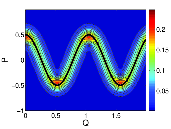
Figure 1. An illustration of the localization of $\sigma(0,Q,P)$ in one dimension for $v_{0}(y)=\frac{\sqrt{2}}{2}\exp\left(\imath\frac{\sin(6y)}{12\varepsilon}\right)$, $\varepsilon=1/128$; the black solid curve is $P=\cos(6Q)/2$.

Define indicator functions $\kappa_{m}$, $m=1,\cdots,M$, which satisfy

(4.21) $$\mathcal{L}_{m}\kappa_{m}=0,$$

with initial condition

(4.22) $$\kappa_{m}(0,\boldsymbol{Q},\boldsymbol{P})=\left\{\begin{array}[]{ll}1&\quad\hbox{if}\;\sigma_{m}(0,\boldsymbol{Q},\boldsymbol{P})\neq 0,\\ 0&\quad\hbox{otherwise}.\end{array}\right.$$

Then in Step 3 of the algorithm, when solving (4.3), (4.4) and (4.6) one only needs to update function values on those $(\boldsymbol{Q^{k}},\boldsymbol{P^{\ell}})$ where $\kappa_{m}$ is nonzero.

Remark.

1. In setting up the meshes, we assume that initial condition either has compact support or decays sufficiently fast to zero as $\boldsymbol{x}\rightarrow\infty$ so that we only need finite number of mesh points in space.

2. The role of the truncation function $r_{\theta}$ is to save computational cost, since although Gaussian function is not localized, it decays quickly away from the center. In practice we take $\theta=\mathcal{O}(\sqrt{\varepsilon})$, the same order as the width of each Gaussian, when evaluate (4.7) and (4.1) numerically.

3. There are two types of errors present in the method. The first type comes from the asymptotic approximation to strictly hyperbolic system. This error can not be reduced unless one includes higher order asymptotic corrections. The other type is the numerical error which comes from two sources: one is from solving the Liouville equations numerically; the other is from the discrete approximation of integrals (4.7) and (4.1). It can be reduced by either taking small mesh size and time step or using higher order numerical methods.

4. Step $2$ and $4$ can be expedited by making use of discrete fast Gaussian transform, as in [QiYi:app1, QiYi:app2].

4.3.3. Semi-Lagrangian method

Alternatively, one can also use semi-Lagrangian method. This is a type of Lagrangian method based on the Liouville equations (4.3), (4.4) and (4.6), which can be viewed as a local implementation of Eulerian method on an adaptive mesh. Different from the meshes of Eulerian method in Section 4.3.1, the meshes of $(\boldsymbol{Q},\boldsymbol{P})$ in semi-Lagrangian method is determined adaptively from initial conditions, while the meshes of $\boldsymbol{y}$ and $\boldsymbol{x}$ are still the same.

The underlying idea is to first lay down uniform mesh grids of $(\boldsymbol{Q},\boldsymbol{P})$, evolve the grids to time $t$ according to Hamiltonian flow (denoted by $(\boldsymbol{Q}^{t},\boldsymbol{P}^{t})$); then set up uniform mesh grids of $(\boldsymbol{Q},\boldsymbol{P})$ at time $t$ based on $(\boldsymbol{Q}^{t},\boldsymbol{P}^{t})$ and use method of characteristics to compute the solutions to the Liouville equations. The difference from Eulerian method is that it solves the Liouville equations by numerical integrators for ODE instead of numerical schemes for PDE. The detailed algorithm is given as follows, where we only focus on computation of one eigenvalue branch and omit the subscript $m$ for simplicity and clarity.

• Choose initial uniform mesh grids $(\boldsymbol{Q}^{\boldsymbol{s},0},\boldsymbol{P}^{\boldsymbol{r},0})$ where $\sigma(0,\boldsymbol{Q}^{\boldsymbol{s},0},\boldsymbol{P}^{\boldsymbol{r},0})$ is nonzero. Solve time-forward Hamiltonian flow

  $$\begin{cases}\displaystyle\frac{\,\mathrm{d}\boldsymbol{Q}}{\,\mathrm{d}t}=\partial_{\boldsymbol{P}}H(\boldsymbol{Q},\boldsymbol{P}),\\[10.00002pt] \displaystyle\frac{\,\mathrm{d}\boldsymbol{P}}{\,\mathrm{d}t}=-\partial_{\boldsymbol{Q}}H(\boldsymbol{Q},\boldsymbol{P}),\end{cases}$$

  with initial conditions

  $$\boldsymbol{Q}(0,\boldsymbol{Q}^{\boldsymbol{s},0},\boldsymbol{P}^{\boldsymbol{r},0})=\boldsymbol{Q}^{\boldsymbol{s},0},\quad\text{and}\quad\boldsymbol{P}(0,\boldsymbol{Q}^{\boldsymbol{s},0},\boldsymbol{P}^{\boldsymbol{r},0})=\boldsymbol{P}^{\boldsymbol{r},0}.$$

  Denote $\big{(}\boldsymbol{Q}^{\boldsymbol{s},t},\boldsymbol{P}^{\boldsymbol{r},t}\big{)}=\big{(}\boldsymbol{Q}(t,\boldsymbol{Q}^{\boldsymbol{s},0},\boldsymbol{P}^{\boldsymbol{r},0}),\boldsymbol{P}(t,\boldsymbol{Q}^{\boldsymbol{s},0},\boldsymbol{P}^{\boldsymbol{r},0})\big{)}$.

• Choose uniform mesh grids $(\boldsymbol{Q^{k}},\boldsymbol{P^{\ell}})$ so that all the points $\big{(}\boldsymbol{Q}^{\boldsymbol{s},t},\boldsymbol{P}^{\boldsymbol{r},t}\big{)}$ lie in mesh cells. Solve time-backward Hamiltonian flow

  $$\begin{cases}\displaystyle\frac{\,\mathrm{d}\boldsymbol{Q}}{\,\mathrm{d}t}=-\partial_{\boldsymbol{P}}H(\boldsymbol{P},\boldsymbol{Q}),\\[10.00002pt] \displaystyle\frac{\,\mathrm{d}\boldsymbol{P}}{\,\mathrm{d}t}=\partial_{\boldsymbol{Q}}H(\boldsymbol{P},\boldsymbol{Q}),\end{cases}$$

  with initial conditions

  $$\boldsymbol{Q}(0,\boldsymbol{Q^{k}},\boldsymbol{P^{\ell}})=\boldsymbol{Q^{k}},\quad\text{and}\quad\boldsymbol{P}(0,\boldsymbol{Q^{k}},\boldsymbol{P^{\ell}})=\boldsymbol{P^{\ell}}.$$

  In the meantime, solve time-backward equation

  $$\frac{\,\mathrm{d}\widetilde{S}}{\,\mathrm{d}t}=-\boldsymbol{P}\cdot\partial_{\boldsymbol{P}}H+H,$$

  with initial condition $\widetilde{S}(0,\boldsymbol{Q^{k}},\boldsymbol{P^{\ell}})=0$, then

  $$S(t,\boldsymbol{Q^{k}},\boldsymbol{P^{\ell}})=-\widetilde{S}(t,\boldsymbol{Q^{k}},\boldsymbol{P^{\ell}}).$$

  Denote $\big{(}\boldsymbol{q^{k}},\boldsymbol{p^{\ell}}\big{)}=\big{(}\boldsymbol{Q}(t,\boldsymbol{Q^{k}},\boldsymbol{P^{\ell}}),\boldsymbol{P}(t,\boldsymbol{Q^{k}},\boldsymbol{P^{\ell}})\big{)}$, then

  $$\boldsymbol{\phi}(t,\boldsymbol{Q^{k}},\boldsymbol{P^{\ell}})=\boldsymbol{p^{\ell}}+\imath\boldsymbol{q^{k}}.$$

• Solve time-forward equation

  $$\frac{\,\mathrm{d}\widetilde{\sigma}}{\,\mathrm{d}t}+\widetilde{\sigma}\boldsymbol{L}^{\mathrm{T}}(\partial_{\boldsymbol{P}}H\cdot\partial_{\boldsymbol{Q}}\boldsymbol{R}-\partial_{\boldsymbol{Q}}H\cdot\partial_{\boldsymbol{P}}\boldsymbol{R})+\widetilde{\sigma}(\partial_{z_{k}}\boldsymbol{L})^{\mathrm{T}}\boldsymbol{F}_{j}Z_{jk}^{-1}\\ +\widetilde{\sigma}\partial_{z_{n}}Q_{j}Z_{kn}^{-1}\boldsymbol{L}^{\mathrm{T}}\bigl{(}-\partial_{Q_{j}}A_{k}+\frac{\imath}{2}P_{l}\partial_{Q_{j}}\partial_{Q_{k}}A_{l}\bigr{)}\boldsymbol{R}=0,$$

  where

  $$\boldsymbol{F}_{j}=-\Bigl{(}(A_{j}-\partial_{P_{j}}H)+\imath(\partial_{Q_{j}}H-P_{l}\partial_{Q_{j}}A_{l})\Bigr{)}\boldsymbol{R},$$

  with initial condition

  $$\widetilde{\sigma}(0,\boldsymbol{q^{k}},\boldsymbol{p^{\ell}})=2^{d/2}\int v_{0}(\boldsymbol{y},\boldsymbol{q^{k}},\boldsymbol{p^{\ell}})\\ \times\exp\bigg{(}\frac{\imath}{\varepsilon}\big{(}-\boldsymbol{p^{\ell}}\cdot(\boldsymbol{y}-\boldsymbol{q^{k}})+\frac{\imath}{2}\lvert\boldsymbol{y}-\boldsymbol{q^{k}}\rvert^{2}\big{)}\bigg{)}\,\mathrm{d}\boldsymbol{y}.$$

  Then $\sigma(t,\boldsymbol{Q^{k}},\boldsymbol{P^{\ell}})=\widetilde{\sigma}(t,\boldsymbol{q^{k}},\boldsymbol{p^{\ell}})$.

• Reconstruct the solution by

  $$\boldsymbol{u}^{\mathrm{SLFGA}}(t,\boldsymbol{x^{n}}) =\sum_{\boldsymbol{k,\ell}}\biggl{(}\frac{\sigma^{\boldsymbol{k,\ell}}}{(2\pi\varepsilon)^{3d/2}}e^{\frac{\imath}{\varepsilon}\big{(}S^{\boldsymbol{k,\ell}}+\boldsymbol{P}^{\boldsymbol{\ell}}\cdot(\boldsymbol{x}^{\boldsymbol{n}}-\boldsymbol{Q^{k}})\big{)}-\frac{1}{2\varepsilon}\lvert\boldsymbol{x}^{\boldsymbol{n}}-\boldsymbol{Q^{k}}\rvert^{2}}\biggr{)}$$

  $$\qquad\times\boldsymbol{R}(\boldsymbol{Q^{k}},\boldsymbol{P^{\ell}})r_{\theta}(\lvert\boldsymbol{x}^{\boldsymbol{n}}-\boldsymbol{Q^{k}}\rvert)\delta Q_{1}\cdots\delta Q_{d}\delta P_{1}\cdots\delta P_{d},$$

  where $\boldsymbol{R}$ the right eigenfunction in (2.3).

Remark.

In Step 3 one needs to compute $Z=\partial_{\boldsymbol{z}}(\boldsymbol{Q}+\imath\boldsymbol{P})$. Since $(\boldsymbol{q^{k}},\boldsymbol{p^{\ell}})$ is not a uniform mesh grid, it can lose accuracy by using divided difference to compute $\partial_{\boldsymbol{z}}\boldsymbol{Q}$ and $\partial_{\boldsymbol{z}}\boldsymbol{P}$. To resolve this problem, one can solve (4.15) to get $\partial_{\boldsymbol{z}}\boldsymbol{Q}$ and $\partial_{\boldsymbol{z}}\boldsymbol{P}$ instead.

4.4. Eulerian method for the Herman-Kluk propagator of the Schrödinger equation

The Eulerian method introduced in Section 4.1 can be also applied to computation of the Herman-Kluk propagator in quantum mechanics.

The rescaled linear Schrödinger equation is given by

(4.23) $$i\varepsilon\frac{\partial\Psi^{\varepsilon}}{\partial t}=-\frac{\varepsilon^{2}}{2}\Delta\Psi^{\varepsilon}+U(\boldsymbol{x})\Psi^{\varepsilon},\quad\boldsymbol{x}\in\mathbb{R}^{d}\,,$$

where $\Psi^{\varepsilon}(t,\boldsymbol{x})$ is the wave function, $U(\boldsymbol{x})$ is the potential and $\varepsilon$ is the re-scaled Plank constant that describes the ratio between quantum time/space scale and the macroscopic time/space scale. This scaling corresponds to the semiclassical regime.

We briefly describe the formulation of the Herman-Kluk propagator [HeKl:84] below. One can see that it is similar to the frozen Gaussian approximation. In fact, the frozen Gaussian approximation introduced in [LuYang:CMS] is motivated by the ideas of the Herman-Kluk propagator. We remark that semiclassical approximation underlying the Herman-Kluk propagator has been recently rigorously analyzed by Swart and Rousse [SwRo:09] and Robert [Ro:09].

Using the Herman-Kluk propagator, the solution to the Schrödinger equation is approximated by

(4.24) $$\Psi^{\varepsilon}_{\mathrm{HK}}(t,\boldsymbol{x})=\frac{1}{(2\pi\varepsilon)^{3d/2}}\int a(t,\boldsymbol{q},\boldsymbol{p})e^{\imath\Phi(t,\boldsymbol{x},\boldsymbol{y},\boldsymbol{q},\boldsymbol{p})/\varepsilon}\Psi_{0}^{\varepsilon}(\boldsymbol{y})\,\mathrm{d}\boldsymbol{y}\,\mathrm{d}\boldsymbol{p}\,\mathrm{d}\boldsymbol{q},$$

where $\Psi_{0}^{\varepsilon}$ is the initial condition of (4.23). Here the phase function $\Phi$ is given by

(4.25) $$\Phi(t,\boldsymbol{x},\boldsymbol{y},\boldsymbol{q},\boldsymbol{p})=S(t,\boldsymbol{q},\boldsymbol{p})+\frac{\imath}{2}\lvert\boldsymbol{x}-\boldsymbol{Q}\rvert^{2}+\boldsymbol{P}\cdot(\boldsymbol{x}-\boldsymbol{Q})\\ +\frac{\imath}{2}\lvert\boldsymbol{y}-\boldsymbol{q}\rvert^{2}-\boldsymbol{p}\cdot(\boldsymbol{y}-\boldsymbol{q}).$$

The evolution of $(\boldsymbol{Q},\boldsymbol{P})$ satisfies

(4.26) $$\begin{cases}\displaystyle\frac{\,\mathrm{d}\boldsymbol{Q}}{\,\mathrm{d}t}=\boldsymbol{P},\\[10.00002pt] \displaystyle\frac{\,\mathrm{d}\boldsymbol{P}}{\,\mathrm{d}t}=-\partial_{\boldsymbol{Q}}U,\end{cases}$$

with initial conditions

(4.27) $$\boldsymbol{Q}(0,\boldsymbol{q},\boldsymbol{p})=\boldsymbol{q},\quad\text{and}\quad\boldsymbol{P}(0,\boldsymbol{q},\boldsymbol{p})=\boldsymbol{p}.$$

The action function $S(t,\boldsymbol{q},\boldsymbol{p})$ satisfies

(4.28) $$\frac{\,\mathrm{d}S}{\,\mathrm{d}t}=\frac{\lvert\boldsymbol{P}\rvert^{2}}{2}-U(\boldsymbol{Q}),$$

with initial condition $S(0,\boldsymbol{q},\boldsymbol{p})=0$. The evolution of ${a}(t,\boldsymbol{q},\boldsymbol{p})$ satisfies

(4.29) $$\frac{\,\mathrm{d}a}{\,\mathrm{d}t}=\frac{1}{2}a\operatorname{tr}\bigg{(}Z^{-1}\big{(}\partial_{\boldsymbol{z}}\boldsymbol{P}-\imath\partial_{\boldsymbol{z}}\boldsymbol{Q}\partial_{\boldsymbol{Q}}^{2}U\big{)}\bigg{)},$$

with initial condition ${a}(0,\boldsymbol{q},\boldsymbol{p})=2^{d/2}$.

It is easy to see that (4.26) and (4.28) are the same as (2.6) and (2.8) if one takes $H_{m}(\boldsymbol{Q},\boldsymbol{P})={\lvert\boldsymbol{P}\rvert^{2}}/{2}+U(\boldsymbol{Q})$. The difference lies in the amplitude evolution equation (4.29). But it does not raise any difficulty for Eulerian formulation. One can still write down Eulerian formulation based on Theorem 4.1,

(4.30) $${\Psi}^{\varepsilon}_{\mathrm{EHK}}(t,\boldsymbol{x})=\frac{1}{(2\pi\varepsilon)^{3d/2}}\int{a}(t,\boldsymbol{Q},\boldsymbol{P})e^{\imath\Theta/\varepsilon}J^{-1}\,\mathrm{d}\boldsymbol{P}\,\mathrm{d}\boldsymbol{Q},$$

where the phase function $\Theta$ is

(4.31) $$\Theta(t,\boldsymbol{x},\boldsymbol{Q},\boldsymbol{P})=S(t,\boldsymbol{Q},\boldsymbol{P})+\boldsymbol{P}\cdot(\boldsymbol{x}-\boldsymbol{Q})+\frac{\imath}{2}\lvert\boldsymbol{x}-\boldsymbol{Q}\rvert^{2}.$$

Define the Liouville operator

$$\mathcal{L}=\partial_{t}+\boldsymbol{P}\cdot\partial_{\boldsymbol{Q}}-\partial_{\boldsymbol{Q}}U\cdot\partial_{\boldsymbol{P}}.$$

Then the evolution of $S(t,\boldsymbol{Q},\boldsymbol{P})$ satisfies

(4.32) $$\mathcal{L}S=\frac{\lvert\boldsymbol{P}\rvert^{2}}{2}-U(\boldsymbol{Q}),$$

with initial condition $S(0,\boldsymbol{Q},\boldsymbol{P})=0$. We introduce the auxiliary function $\boldsymbol{\phi}(t,\boldsymbol{Q},\boldsymbol{P})$, which satisfies

(4.33) $$\mathcal{L}\boldsymbol{\phi}=0,$$

with initial condition

(4.34) $$\boldsymbol{\phi}(0,\boldsymbol{Q},\boldsymbol{P})=\boldsymbol{P}+\imath\boldsymbol{Q}.$$

With $\boldsymbol{\phi}$ determined, the evolution of $a(t,\boldsymbol{Q},\boldsymbol{P})$ satisfies

(4.35) $$\mathcal{L}a=-\frac{1}{2}a\operatorname{tr}\bigg{(}Z^{-1}\big{(}(\partial_{\boldsymbol{Q}}\boldsymbol{\phi})^{\mathrm{T}}+\imath(\partial_{\boldsymbol{P}}\boldsymbol{\phi})^{\mathrm{T}}\partial_{\boldsymbol{Q}}^{2}U\big{)}\bigg{)},$$

where

(4.36) $$Z=\bigl{(}\partial_{\boldsymbol{P}}\boldsymbol{\phi}\bigr{)}^{\mathrm{T}}-\imath\bigl{(}\partial_{\boldsymbol{Q}}\boldsymbol{\phi}\bigr{)}^{\mathrm{T}}.$$

The initial condition of (4.35) is prepared as

(4.37) $$a(0,\boldsymbol{Q},\boldsymbol{P})=2^{d/2}\int\Psi^{\varepsilon}_{0}(\boldsymbol{y})\exp\bigg{(}\frac{\imath}{\varepsilon}\big{(}-\boldsymbol{P}\cdot(\boldsymbol{y}-\boldsymbol{Q})+\frac{\imath}{2}\lvert\boldsymbol{y}-\boldsymbol{Q}\rvert^{2}\big{)}\bigg{)}\,\mathrm{d}\boldsymbol{y}.$$

Therefore the numerical methods discussed in section 4.3 can also be applied to the Herman-Kluk propagator.

5. Numerical examples

In this section, we present four numerical examples to show the performance of Eulerian frozen Gaussian approximation (EFGA) and also Eulerian methods for the Herman-Kluk propagator. Two of the examples correspond to EFGA of wave propagation discussed in Section 2.3, and the other corresponds to the Schrödinger equation discussed in Section 4.4. We consider WKB initial conditions, and use the Eulerian method with local indicator to compute wave propagation, and use the semi-Lagrangian method for the Herman-Kluk propagator of the Schrödinger equation.

5.1. Wave propagation

Example 5.1 (One-dimensional scalar wave equation).

$$\partial_{t}^{2}u-c(x)^{2}\partial_{x}^{2}u=0.$$

The wave speed is $c(x)=x^{2}$. The initial conditions are

$$u_{0}=\exp\bigl{(}-100(x-0.5)^{2}\bigr{)}\exp\left(\frac{\imath x}{\varepsilon}\right),$$

$$\partial_{t}u_{0}=-\frac{\imath x^{2}}{\varepsilon}\exp\bigl{(}-100(x-0.5)^{2}\bigr{)}\exp\left(\frac{\imath x}{\varepsilon}\right).$$

The final time is $T=0.8$. We plot the real part of the wave field obtained by EFGA compared with the true solution in Figure 2 for $\varepsilon=1/64,\;1/128,\;1/256$. As one can see, the span of the solution reaches $2$ roughly at $T=0.8$, although it starts with only $0.5$ approximately. Apparently the wave spreads quickly in this example. Table 1 shows the $\ell^{\infty}$ and $\ell^{2}$ errors of the EFGA solution. The convergence orders in $\varepsilon$ of $\ell^{\infty}$ and $\ell^{2}$ norms are $1.02$ and $1.20$ separately for EFGA, which confirms the asymptotic accuracy. The true solution is computed by the finite difference method using the mesh size of $N_{x}=49152$ and the time step of $N_{t}=524288$ for domain $[0,6]$. We take $N_{t}=1024$, $\delta q=\delta p=\delta y=1/128$ and $\delta x=1/2048$ in EFGA.

Table 1. Example 5.1, the $\ell^{\infty}$ and $\ell^{2}$ errors for EFGA.

$\varepsilon$	${1}/{2^{6}}$	${1}/{2^{7}}$	${1}/{2^{8}}$
$\lVert u-u^{\mathrm{EFGA}}\rVert_{\ell^{\infty}}$	$1.46\times 10^{-1}$	$6.39\times 10^{-2}$	$3.52\times 10^{-2}$
$\lVert u-u^{\mathrm{EFGA}}\rVert_{\ell^{2}}$	$4.81\times 10^{-2}$	$2.39\times 10^{-2}$	$9.11\times 10^{-3}$

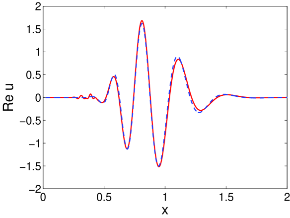
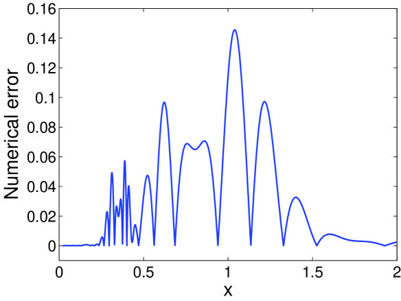
(a) $\varepsilon=\frac{1}{64}$
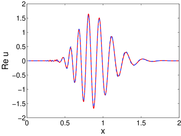
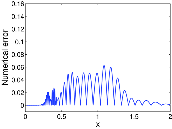
(b) $\varepsilon=\frac{1}{128}$
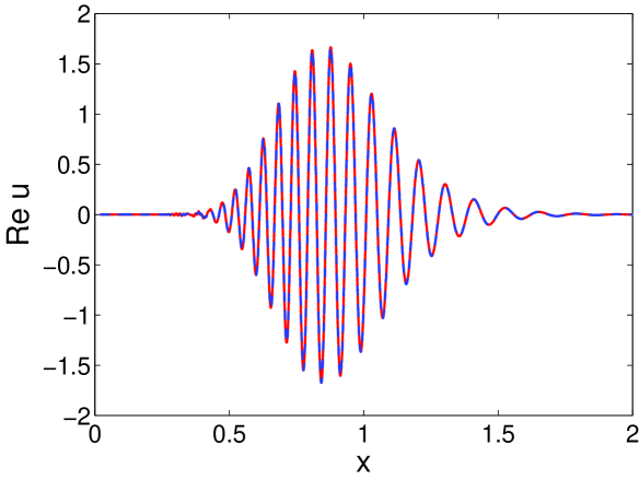
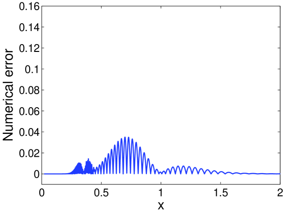
(c) $\varepsilon=\frac{1}{256}$

Figure 2. Example 5.1, the comparison of the true solution (solid line) and the solution by EFGA (dash line). Left: the real part of wave field; right: the errors between them.

Example 5.2 (Two-dimensional acoustic wave equations).

$$\begin{cases}\partial_{t}\boldsymbol{V}+\nabla\Pi=0;\\ \partial_{t}\Pi+c^{2}(\boldsymbol{x})\nabla\cdot\boldsymbol{V}=0,\end{cases}$$

where $\boldsymbol{V}=(V_{1},V_{2})$, $\boldsymbol{x}=(x_{1},x_{2})$ and $c(\boldsymbol{x})=1$. The initial conditions are

$$\Pi_{0}=\sqrt{1+\sin^{2}(4x_{2})/16}\exp\bigl{(}-100(x_{1}^{2}+x_{2}^{2})\bigr{)}\exp\left(\frac{\imath}{\varepsilon}\big{(}-x_{1}+\cos(4x_{2})/16\big{)}\right),$$

$$V_{1,0}=-\exp\bigl{(}-100(x_{1}^{2}+x_{2}^{2})\bigr{)}\exp\left(\frac{\imath}{\varepsilon}\big{(}-x_{1}+\cos(4x_{2})/16\big{)}\right),$$

$$V_{2,0}=-\frac{\sin(4x_{2})}{4}\exp\bigl{(}-100(x_{1}^{2}+x_{2}^{2})\bigr{)}\exp\left(\frac{\imath}{\varepsilon}\big{(}-x_{1}+\cos(4x_{2})/16\big{)}\right).$$

The final time is $T=1.0$. We take $\varepsilon=1/64$. Figure 3 compares the pressure $\Pi$ of the true solution with the one by EFGA. Figure 4 compares the velocity $\boldsymbol{V}$ of the true solution with the one by EFGA. It is clear that EFGA can provide a good approximation to both the pressure and velocity for acoustic wave propagation in two dimension. The true solution is given by the spectral method using the mesh $\delta x_{1}=\delta x_{2}=1/512$ for domain $[-1.5,0.5]\times[-1,1]$. We take $\delta q_{1}=\delta q_{2}=\delta p_{1}=\delta p_{2}=\delta y_{1}=\delta y_{2}=1/32$ and $\delta x_{1}=\delta x_{2}=1/64$ in EFGA.

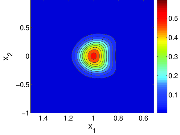
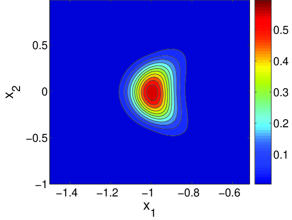
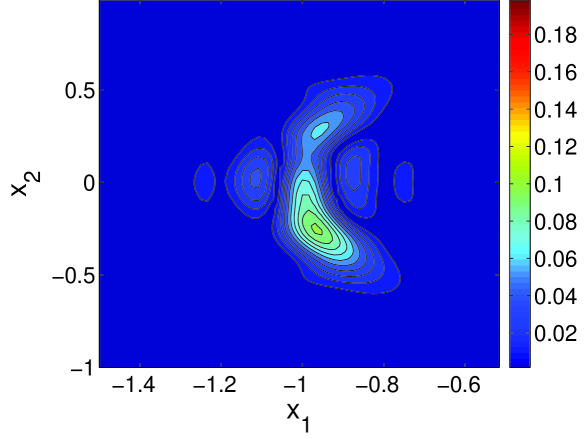
Figure 3. Example 5.2, the comparison of the true solution and the solution by EFGA. Top (left): pressure of EFGA; top (right): pressure of true solution; bottom: the error between them.

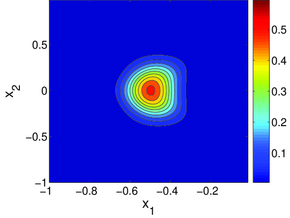
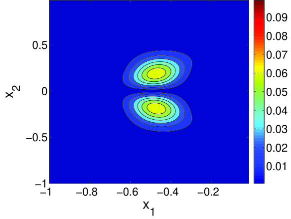
(a) Eulerian Frozen Gaussian approximation
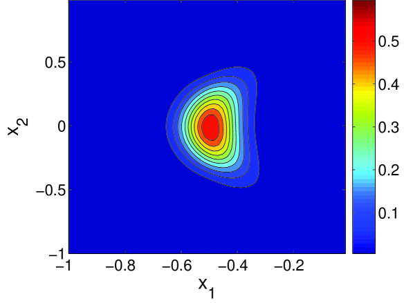
(b) True solution
(c) Errors

Figure 4. Example 5.2, the comparison of the true solution and the solution by EFGA. Left: velocity component $V_{1}$; right: velocity component $V_{2}$.

5.2. Schrödinger equation

Example 5.3 (One-dimensional Schrödinger equation).

$$i\varepsilon\frac{\partial\Psi^{\varepsilon}}{\partial t}=-\frac{\varepsilon^{2}}{2}\Delta\Psi^{\varepsilon},\quad{x}\in\mathbb{R}\,,$$

and the initial condition is

$$\Psi_{0}^{\varepsilon}=\exp\left(-\imath\frac{x}{\varepsilon}-\frac{x^{2}}{2\varepsilon}\right).$$

We use this one-dimensional Schrödinger equation with zero potential as an example to compare the performance of Lagrangian and Eulerian methods. The true solution can be given analytically,

$$\Psi^{\varepsilon}(t,x)=\frac{1}{1+t\imath}\exp\biggl{(}\frac{\imath}{\varepsilon}\Bigl{(}x-\frac{t}{2}+\frac{(t+\imath)(x-t)^{2}}{2(1+t^{2})}\Bigr{)}\biggr{)},$$

which implies the solution spreads as time increases.

We choose $\varepsilon=1/128$ and evolve the equation up to $T=10$. The mesh sizes are $\delta x=\delta y=\delta q=\delta p=1/64$. We take $N_{q}=64$ and $N_{p}=33$ in the Lagrangian method. The comparison of wave amplitudes and numerical errors are presented in Figure 5. One can see that, when the divergence of particle trajectories occurs, Eulerian method has a much better resolution than the Lagrangian method.

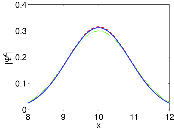
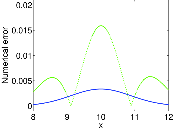
Figure 5. Example 5.3. Left: the wave amplitude comparison of the true solution (dashed line), the Lagrangian method (dots) and the Eulerian method (solid line); right: the numerical errors of the Lagrangian method (dots) and the Eulerian method (solid line).

Example 5.4 (Two-dimensional Schrödinger equation).

$$i\varepsilon\frac{\partial\Psi^{\varepsilon}}{\partial t}=-\frac{\varepsilon^{2}}{2}\Delta\Psi^{\varepsilon}+\frac{1}{2}\lvert\boldsymbol{x}\rvert^{2}\Psi^{\varepsilon},\quad\boldsymbol{x}\in\mathbb{R}^{2}\,,$$

and the initial condition is

$$\Psi_{0}^{\varepsilon}=\exp\bigl{(}-25(x_{1}^{2}+x_{2}^{2})\bigr{)}\exp\left(\frac{\imath}{2\varepsilon}\sin(x_{1})\sin(x_{2})\right).$$

This is an example of Schrödinger equation in two dimension, which describes the dynamics of electron under harmonic potential. We take $\varepsilon=1/128$. Figure 6 compares the wave amplitude of the true solution with the numerical one at time $T=0.5$ and $T=1$. This shows that Eulerian Herman-Kluk propagator has good performances in both cases of solution spreading and localizing. The true solution is given by the spectral method using the mesh $\delta x_{1}=\delta x_{2}=1/512$ for domain $[-1,1]\times[-1,1]$. In the numerical approximation, the mesh sizes are chosen to be $\delta q_{1}=\delta q_{2}=\delta p_{1}=\delta p_{2}=\delta y_{1}=\delta y_{2}=1/32$ in discretization of integrals and $\delta x_{1}=\delta x_{2}=1/32$ in reconstruction of solution.

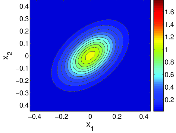
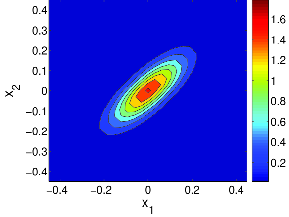
(a) Eulerian Herman-Kluk propagator
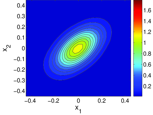
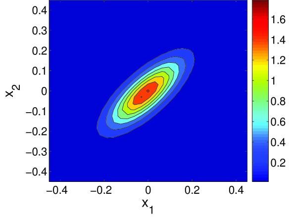
(b) True solution
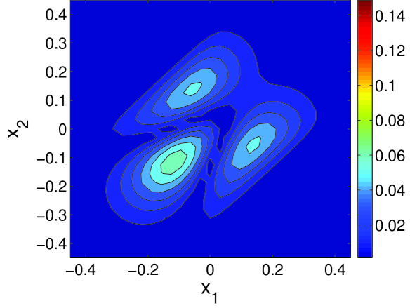
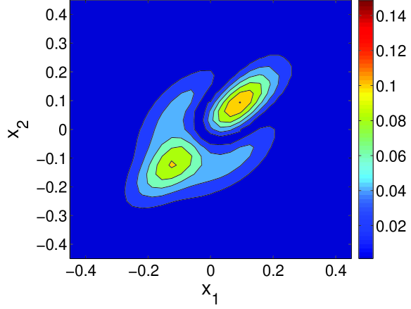
(c) Errors

Figure 6. Example 5.4, the comparison of the true solution and the solution by Eulerian Herman-Kluk propagator. Left: $T=0.5$; right: $T=1$.

6. Conclusion

We extend the formulation of frozen Gaussian approximation to general linear strictly hyperbolic system. Based on the Eulerian formulation of frozen Gaussian approximation, Eulerian methods are developed to resolve the divergence problem of the Lagrangian method. Moreover, the Eulerian methods can be also used for computing the Herman-Kluk propagator of the Schrödinger equation in quantum mechanics. The performance of the proposed methods is verified by numerical examples. This paper, together with [LuYang:CMS], provides an efficient methodology for computing high frequency wave propagation for general hyperbolic systems with smooth coefficient.