Frozen Gaussian approximation for high frequency wave propagation

Jianfeng Lu Department of Mathematics
Courant Institute of Mathematical Sciences
New York University
New York, NY 10012
email: jianfeng@cims.nyu.edu
 and  Xu Yang Program in Applied and Computational Mathematics
Princeton University
Princeton, NJ 08544
email: xuyang@math.princeton.edu
(Date: August 8, 2010. Revised : November 11, 2010)
Abstract.

We propose the frozen Gaussian approximation for computation of high frequency wave propagation. This method approximates the solution to the wave equation by an integral representation. It provides a highly efficient computational tool based on the asymptotic analysis on phase plane. Compared to geometric optics, it provides a valid solution around caustics. Compared to the Gaussian beam method, it overcomes the drawback of beam spreading. We give several numerical examples to verify that the frozen Gaussian approximation performs well in the presence of caustics and when the Gaussian beam spreads. Moreover, it is observed numerically that the frozen Gaussian approximation exhibits better accuracy than the Gaussian beam method.

Both authors are grateful to Weinan E for his inspiration and helpful suggestions and discussions that improve the presentation. J.L. would like to thank Lexing Ying for stimulating discussions and for providing preprints [QiYi:app1, QiYi:app2] before publication. Part of the work was done during J.L.’s visits to Institute of Computational Mathematics and Scientific/Engineering Computing of Chinese Academy of Sciences and Peking University, and X.Y.’s visits to Tsinghua University and Peking University. We appreciate their hospitality. We thank anonymous referees for their valuable suggestions and remarks. X.Y. was partially supported by the DOE grant DE-FG02-03ER25587, the NSF grant DMS-0708026 and the AFOSR grant FA9550-08-1-0433.

1. Introduction

We are interested in developing efficient numerical methods for high frequency wave propagation. For simplicity and clarity we take the following linear scalar wave equation to present the idea,

(1.1) t2uc2(𝒙)Δu=0,𝒙d,formulae-sequencesuperscriptsubscript𝑡2𝑢superscript𝑐2𝒙Δ𝑢0𝒙superscript𝑑\partial_{t}^{2}u-c^{2}(\boldsymbol{x})\Delta u=0,\qquad\boldsymbol{x}\in\mathbb{R}^{d},

with WKB initial conditions,

(1.2) {u0(𝒙)=A0(𝒙)eıεS0(𝒙),tu0(𝒙)=1εB0(𝒙)eıεS0(𝒙),casessubscript𝑢0𝒙subscript𝐴0𝒙superscript𝑒italic-ı𝜀subscript𝑆0𝒙otherwisesubscript𝑡subscript𝑢0𝒙1𝜀subscript𝐵0𝒙superscript𝑒italic-ı𝜀subscript𝑆0𝒙otherwise\begin{cases}u_{0}(\boldsymbol{x})=A_{0}(\boldsymbol{x})e^{\frac{\imath}{\varepsilon}S_{0}(\boldsymbol{x})},\\ \partial_{t}u_{0}(\boldsymbol{x})=\frac{1}{\varepsilon}B_{0}(\boldsymbol{x})e^{\frac{\imath}{\varepsilon}S_{0}(\boldsymbol{x})},\end{cases}

where u𝑢u is the wave field, d𝑑d is the dimensionality and ı=1italic-ı1\imath=\sqrt{-1} is the imaginary unit. We assume that the local wave speed c(𝒙)𝑐𝒙c(\boldsymbol{x}) is a smooth function. The small parameter ε1much-less-than𝜀1\varepsilon\ll 1 characterizes the high frequency nature of the wave. The proposed method can be generalized to other types of wave equations [LuYang:MMS].

Numerical computation of high frequency wave propagation is an important problem arising in many applications, such as electromagnetic radiation and scattering, seismic and acoustic waves traveling, just to name a few. It is a two-scale problem. The large length scale comes from the characteristic size of the medium, while the small length scale is the wavelength. The disparity between the two length scales makes direct numerical computations extremely hard. In order to achieve accurate results, the mesh size has to be chosen comparable to the wavelength or even smaller. On the other hand, the domain size is large so that a huge number of grid points are needed.

In order to compute efficiently high frequency wave propagation, algorithms based on asymptotic analysis have been developed. One of the most famous examples is geometric optics. In the method, it is assumed that the solution has a form of

(1.3) u(t,𝒙)=A(t,𝒙)eıS(t,𝒙)/ε.𝑢𝑡𝒙𝐴𝑡𝒙superscript𝑒italic-ı𝑆𝑡𝒙𝜀u(t,\boldsymbol{x})=A(t,\boldsymbol{x})e^{\imath S(t,\boldsymbol{x})/\varepsilon}.

To the leading order, the phase function S(t,𝒙)𝑆𝑡𝒙S(t,\boldsymbol{x}) satisfies the eikonal equation,

(1.4) |tS|2c2(𝒙)|𝒙S|2=0,superscriptsubscript𝑡𝑆2superscript𝑐2𝒙superscriptsubscript𝒙𝑆20\lvert\partial_{t}S\rvert^{2}-c^{2}(\boldsymbol{x})\lvert\nabla_{\boldsymbol{x}}S\rvert^{2}=0,

and the amplitude A(t,𝒙)𝐴𝑡𝒙A(t,\boldsymbol{x}) satisfies the transport equation,

tAc2(𝒙)𝒙StS𝒙A+(t2Sc2(𝒙)ΔS)2tSA=0.subscript𝑡𝐴superscript𝑐2𝒙subscript𝒙𝑆subscript𝑡𝑆subscript𝒙𝐴superscriptsubscript𝑡2𝑆superscript𝑐2𝒙Δ𝑆2subscript𝑡𝑆𝐴0\partial_{t}A-c^{2}(\boldsymbol{x})\frac{\nabla_{\boldsymbol{x}}S}{\partial_{t}S}\cdot\nabla_{\boldsymbol{x}}A+\frac{\bigl{(}\partial_{t}^{2}S-c^{2}(\boldsymbol{x})\Delta S\bigr{)}}{2\partial_{t}S}A=0.

The merit of geometric optics is that it only solves the macroscopic quantities S(t,𝒙)𝑆𝑡𝒙S(t,\boldsymbol{x}) and A(t,𝒙)𝐴𝑡𝒙A(t,\boldsymbol{x}) which are ε𝜀\varepsilon-independent. Computational methods based on the geometric optics are reviewed in [EnRu:03, Ru:07].

However, since the eikonal equation (1.4) is of Hamilton-Jacobi type, the solution of (1.4) becomes singular after the formation of caustics. At caustics, the approximate solution of geometric optics is invalid since the amplitude A(t,𝒙)𝐴𝑡𝒙A(t,\boldsymbol{x}) blows up. To overcome this problem, Popov introduced Gaussian beam method in [Po:82]. The single beam solution of the Gaussian beam method has a similar form to geometric optics,

u(t,𝒙)=A(t,𝒚)eıS~(t,𝒙,𝒚)/ε.𝑢𝑡𝒙𝐴𝑡𝒚superscript𝑒italic-ı~𝑆𝑡𝒙𝒚𝜀u(t,\boldsymbol{x})=A(t,\boldsymbol{y})e^{\imath\tilde{S}(t,\boldsymbol{x},\boldsymbol{y})/\varepsilon}.

The difference lies in that the Gaussian beam method uses a complex phase function,

(1.5) S~(t,𝒙,𝒚)=S(t,𝒚)+𝒑(t,𝒚)(𝒙𝒚)+12(𝒙𝒚)M(t,𝒚)(𝒙𝒚),~𝑆𝑡𝒙𝒚𝑆𝑡𝒚𝒑𝑡𝒚𝒙𝒚12𝒙𝒚𝑀𝑡𝒚𝒙𝒚\tilde{S}(t,\boldsymbol{x},\boldsymbol{y})=S(t,\boldsymbol{y})+\boldsymbol{p}(t,\boldsymbol{y})\cdot(\boldsymbol{x}-\boldsymbol{y})+\frac{1}{2}(\boldsymbol{x}-\boldsymbol{y})\cdot M(t,\boldsymbol{y})(\boldsymbol{x}-\boldsymbol{y}),

where S,𝒑d,Md×dformulae-sequence𝑆formulae-sequence𝒑superscript𝑑𝑀superscript𝑑𝑑S\in\mathbb{R},\;\boldsymbol{p}\in\mathbb{R}^{d},\;M\in\mathbb{C}^{d\times d}. The imaginary part of M𝑀M is chosen to be positive definite so that the solution decays exponentially away from 𝒙=𝒚𝒙𝒚\boldsymbol{x}=\boldsymbol{y}, where 𝒚𝒚\boldsymbol{y} is called the beam center. This makes the solution a Gaussian function, and hence the method was named the Gaussian beam method. If the initial wave is not in a form of single beam, one can approximate it by using a number of Gaussian beams. The validity of this construction at caustics was analyzed by Ralston in [Ra:82]. Recently, there have been a series of numerical studies including both the Lagrangian type [TaQiRa:07, Ta:08, MoRu:app, QiYi:app1, QiYi:app2] and the Eulerian type [LeQiBu:07, LeQi:09, JiWuYa:08, JiWuYaHu:10, JiWuYa:10, JiWuYa:11, LiRa:09, LiRa:10].

The construction of Gaussian beam approximation is based on the truncation of the Taylor expansion of S~~𝑆\tilde{S} around the beam center 𝒚𝒚\boldsymbol{y} up to the quadratic term, hence it loses accuracy when the width of the beam becomes large, i.e., when the imaginary part of M(t,𝒚)𝑀𝑡𝒚M(t,\boldsymbol{y}) in (1.5) becomes small so that the Gaussian function is not localized any more. This happens for example when the solution of the wave equation spreads (the opposite situation of forming caustics). This is a severe problem in general, as shown by examples in Section 4. One could overcome the problem of spreading of beams by doing reinitialization once in a while, see [QiYi:app1, QiYi:app2]. This increases the computational complexity especially when beams spread quickly.

Therefore a method working in both scenario of spreading and caustics is required. The main idea of the method proposed in the current work is to use Gaussian functions with fixed widths, instead of using those that might spread over time, to approximate the wave solution. That is why this type of method is called frozen Gaussian approximation (FGA). Despite its superficial similarity with the Gaussian beam method (GBM), it is different at a fundamental level. FGA is based on phase plane analysis, while GBM is based on the asymptotic solution to a wave equation with Gaussian initial data. In FGA, the solution to the wave equation is approximated by a superposition of Gaussian functions living in the phase space, and each function is not necessarily an asymptotic solution, while GBM uses Gaussian functions (named as beams) in the physical space, with each individual beam being an asymptotic solution to the wave equation. The main advantage of FGA over GBM is that the problem of beam spreading no longer exists.111Divergence is still an issue for the Lagrangian approach, one needs to work in the Eulerian framework to completely solve the problem, which is considered in [LuYang:MMS]. Besides, numerically we observe that FGA has better accuracy than GBM when keeping the same order of terms in asymptotic series. On the other hand, the solution given by FGA is asymptotically accurate around caustics where geometric optics breaks down.

Our work is motivated by the chemistry literature on the propagation of time dependent Schrödinger equation, where the spreading of solution is a common phenomenon, for example, in the dynamics of a free electron. In [He:81], Heller introduced frozen Gaussian wavepackets to deal with this issue, but it only worked for a short time propagation of order 𝒪()𝒪Planck-constant-over-2-pi\mathcal{O}(\hbar) where Planck-constant-over-2-pi\hbar is the Planck constant. To make it valid for longer time of order 𝒪(1)𝒪1\mathcal{O}(1), Herman and Kluk proposed in [HeKl:84] to change the weight of Gaussian packets by adding so-called Herman-Kluk prefactor. Integral representation and higher order approximations were developed by Kay in [Ka:94] and [Ka:06]. Recently, the semiclassical approximation underlying the method was analyzed rigorously by Swart and Rousse in [SwRo:09] and also Robert in [Ro:09]. We generalize their ideas for propagation of high frequency waves, aiming at developing an efficient computational method. We decompose waves into several branches of propagation, and each of them is approximated using Gaussian functions on phase plane. Their centers follow different Hamiltonian dynamics for different branches. Their weight functions, which are analogous to the Herman-Kluk prefactor, satisfy new evolution equations derived from asymptotic analysis.

The rest of paper is organized as follows. In Section 2, we state the formulations and numerical algorithm of the frozen Gaussian approximation. In Section 3, we provide asymptotic analysis to justify the formulations introduced in Section 2. The numerical examples are given in Section 4 to verify the accuracy and to compare the frozen Gaussian approximation (FGA) with the Gaussian beam method (GBM). In Section 5, we discuss the efficiency of FGA in comparison with GBM and higher order GBM, with some comments on the phenomenon of error cancellation, and we give some conclusive remarks in the end.

2. Formulation and algorithm

In this section we present the basic formulation and the main algorithm of the frozen Gaussian approximation (FGA), and leave the derivation to the next section.

2.1. Formulation

FGA approximates the solution to the wave equation (1.1) by the integral representation,

(2.1) uFGA(t,𝒙)superscript𝑢FGA𝑡𝒙\displaystyle u^{\mathrm{FGA}}(t,\boldsymbol{x}) =1(2πε)3d/23da+(t,𝒒,𝒑)eıεΦ+(t,𝒙,𝒚,𝒒,𝒑)u+,0(𝒚)d𝒚d𝒑d𝒒absent1superscript2𝜋𝜀3𝑑2subscriptsuperscript3𝑑subscript𝑎𝑡𝒒𝒑superscript𝑒italic-ı𝜀subscriptΦ𝑡𝒙𝒚𝒒𝒑subscript𝑢0𝒚differential-d𝒚differential-d𝒑differential-d𝒒\displaystyle=\frac{1}{(2\pi\varepsilon)^{3d/2}}\int_{\mathbb{R}^{3d}}a_{+}(t,\boldsymbol{q},\boldsymbol{p})e^{\frac{\imath}{\varepsilon}\Phi_{+}(t,\boldsymbol{x},\boldsymbol{y},\boldsymbol{q},\boldsymbol{p})}u_{+,0}(\boldsymbol{y})\,\mathrm{d}\boldsymbol{y}\,\mathrm{d}\boldsymbol{p}\,\mathrm{d}\boldsymbol{q}
+1(2πε)3d/23da(t,𝒒,𝒑)eıεΦ(t,𝒙,𝒚,𝒒,𝒑)u,0(𝒚)d𝒚d𝒑d𝒒,1superscript2𝜋𝜀3𝑑2subscriptsuperscript3𝑑subscript𝑎𝑡𝒒𝒑superscript𝑒italic-ı𝜀subscriptΦ𝑡𝒙𝒚𝒒𝒑subscript𝑢0𝒚differential-d𝒚differential-d𝒑differential-d𝒒\displaystyle+\frac{1}{(2\pi\varepsilon)^{3d/2}}\int_{\mathbb{R}^{3d}}a_{-}(t,\boldsymbol{q},\boldsymbol{p})e^{\frac{\imath}{\varepsilon}\Phi_{-}(t,\boldsymbol{x},\boldsymbol{y},\boldsymbol{q},\boldsymbol{p})}u_{-,0}(\boldsymbol{y})\,\mathrm{d}\boldsymbol{y}\,\mathrm{d}\boldsymbol{p}\,\mathrm{d}\boldsymbol{q},

where u±,0subscript𝑢plus-or-minus0u_{\pm,0} are determined by the initial value,

(2.2) u±,0(𝒙)=A±(𝒙)eıεS0(𝒙),subscript𝑢plus-or-minus0𝒙subscript𝐴plus-or-minus𝒙superscript𝑒italic-ı𝜀subscript𝑆0𝒙u_{\pm,0}(\boldsymbol{x})=A_{\pm}(\boldsymbol{x})e^{\frac{\imath}{\varepsilon}S_{0}(\boldsymbol{x})},

with

A±(𝒙)=12(A0(𝒙)±ıB0(𝒙)c(𝒙)|𝒙S0(𝒙)|).subscript𝐴plus-or-minus𝒙12plus-or-minussubscript𝐴0𝒙italic-ısubscript𝐵0𝒙𝑐𝒙subscript𝒙subscript𝑆0𝒙A_{\pm}(\boldsymbol{x})=\frac{1}{2}\biggl{(}A_{0}(\boldsymbol{x})\pm\frac{\imath B_{0}(\boldsymbol{x})}{c(\boldsymbol{x})\lvert\partial_{\boldsymbol{x}}S_{0}(\boldsymbol{x})\rvert}\biggr{)}.

The equation (2.1) implies that the solution consists of two branches (“±plus-or-minus\pm”).

In (2.1), Φ±subscriptΦplus-or-minus\Phi_{\pm} are the phase functions given by

(2.3) Φ±(t,𝒙,𝒚,𝒒,𝒑)=𝑷±(t,𝒒,𝒑)(𝒙𝑸±(t,𝒒,𝒑))𝒑(𝒚𝒒)+ı2|𝒙𝑸±(t,𝒒,𝒑)|2+ı2|𝒚𝒒|2.subscriptΦplus-or-minus𝑡𝒙𝒚𝒒𝒑subscript𝑷plus-or-minus𝑡𝒒𝒑𝒙subscript𝑸plus-or-minus𝑡𝒒𝒑𝒑𝒚𝒒italic-ı2superscript𝒙subscript𝑸plus-or-minus𝑡𝒒𝒑2italic-ı2superscript𝒚𝒒2\Phi_{\pm}(t,\boldsymbol{x},\boldsymbol{y},\boldsymbol{q},\boldsymbol{p})=\boldsymbol{P}_{\pm}(t,\boldsymbol{q},\boldsymbol{p})\cdot(\boldsymbol{x}-\boldsymbol{Q}_{\pm}(t,\boldsymbol{q},\boldsymbol{p}))-\boldsymbol{p}\cdot(\boldsymbol{y}-\boldsymbol{q})\\ +\frac{\imath}{2}\lvert\boldsymbol{x}-\boldsymbol{Q}_{\pm}(t,\boldsymbol{q},\boldsymbol{p})\rvert^{2}+\frac{\imath}{2}\lvert\boldsymbol{y}-\boldsymbol{q}\rvert^{2}.

Given 𝒒𝒒\boldsymbol{q} and 𝒑𝒑\boldsymbol{p} as parameters, the evolution of 𝑸±subscript𝑸plus-or-minus\boldsymbol{Q}_{\pm} and 𝑷±subscript𝑷plus-or-minus\boldsymbol{P}_{\pm} are given by the equation of motion corresponding to the Hamiltonian H±=±c(𝑸±)|𝑷±|subscript𝐻plus-or-minusplus-or-minus𝑐subscript𝑸plus-or-minussubscript𝑷plus-or-minusH_{\pm}=\pm c(\boldsymbol{Q}_{\pm})\lvert\boldsymbol{P}_{\pm}\rvert,

(2.4) {d𝑸±dt=𝑷±H±=±c𝑷±|𝑷±|,d𝑷±dt=𝑸±H±=𝑸±c|𝑷±|,casesdsubscript𝑸plus-or-minusd𝑡subscriptsubscript𝑷plus-or-minussubscript𝐻plus-or-minusplus-or-minus𝑐subscript𝑷plus-or-minussubscript𝑷plus-or-minusotherwisedsubscript𝑷plus-or-minusd𝑡subscriptsubscript𝑸plus-or-minussubscript𝐻plus-or-minusminus-or-plussubscriptsubscript𝑸plus-or-minus𝑐subscript𝑷plus-or-minusotherwise\begin{cases}\displaystyle\frac{\,\mathrm{d}\boldsymbol{Q}_{\pm}}{\,\mathrm{d}t}=\partial_{\boldsymbol{P}_{\pm}}H_{\pm}=\pm c\frac{\boldsymbol{P}_{\pm}}{\lvert\boldsymbol{P}_{\pm}\rvert},\\ \displaystyle\frac{\,\mathrm{d}\boldsymbol{P}_{\pm}}{\,\mathrm{d}t}=-\partial_{\boldsymbol{Q}_{\pm}}H_{\pm}=\mp\partial_{\boldsymbol{Q}_{\pm}}c\lvert\boldsymbol{P}_{\pm}\rvert,\end{cases}

with the initial conditions 𝑸±(0,𝒒,𝒑)=𝒒subscript𝑸plus-or-minus0𝒒𝒑𝒒\boldsymbol{Q}_{\pm}(0,\boldsymbol{q},\boldsymbol{p})=\boldsymbol{q} and 𝑷±(0,𝒒,𝒑)=𝒑subscript𝑷plus-or-minus0𝒒𝒑𝒑\boldsymbol{P}_{\pm}(0,\boldsymbol{q},\boldsymbol{p})=\boldsymbol{p}. The evolution equation of a±subscript𝑎plus-or-minusa_{\pm} is given by

(2.5) da±dtdsubscript𝑎plus-or-minusd𝑡\displaystyle\frac{\,\mathrm{d}a_{\pm}}{\,\mathrm{d}t} =±a±2(𝑷±|𝑷±|𝑸±c(d1)ı|𝑷±|c)absentplus-or-minussubscript𝑎plus-or-minus2subscript𝑷plus-or-minussubscript𝑷plus-or-minussubscriptsubscript𝑸plus-or-minus𝑐𝑑1italic-ısubscript𝑷plus-or-minus𝑐\displaystyle=\pm\frac{a_{\pm}}{2}\Bigl{(}\frac{\boldsymbol{P}_{\pm}}{\lvert\boldsymbol{P}_{\pm}\rvert}\cdot\partial_{\boldsymbol{Q}_{\pm}}c-\frac{(d-1)\imath}{\lvert\boldsymbol{P}_{\pm}\rvert}c\Bigr{)}
±a±2tr(Z±1𝒛𝑸±(2𝑷±|𝑷±|𝑸±c\displaystyle\pm\frac{a_{\pm}}{2}\operatorname{tr}\biggl{(}Z_{\pm}^{-1}\partial_{\boldsymbol{z}}\boldsymbol{Q}_{\pm}\Bigl{(}2\frac{\boldsymbol{P}_{\pm}}{\lvert\boldsymbol{P}_{\pm}\rvert}\otimes\partial_{\boldsymbol{Q}_{\pm}}c
ıc|𝑷±|(𝑷±𝑷±|𝑷±|2I)ı|𝑷±|𝑸±2c))\displaystyle\hskip 60.00009pt-\frac{\imath c}{\lvert\boldsymbol{P}_{\pm}\rvert}\Bigl{(}\frac{\boldsymbol{P}_{\pm}\otimes\boldsymbol{P}_{\pm}}{\lvert\boldsymbol{P}_{\pm}\rvert^{2}}-I\Bigr{)}-\imath\lvert\boldsymbol{P}_{\pm}\rvert\partial_{\boldsymbol{Q}_{\pm}}^{2}c\Bigr{)}\biggr{)}

with the initial condition,

a±(0,𝒒,𝒑)=2d/2.subscript𝑎plus-or-minus0𝒒𝒑superscript2𝑑2a_{\pm}(0,\boldsymbol{q},\boldsymbol{p})=2^{d/2}.

In (2.5), 𝑷±subscript𝑷plus-or-minus\boldsymbol{P}_{\pm} and 𝑸±subscript𝑸plus-or-minus\boldsymbol{Q}_{\pm} are evaluated at (t,𝒒,𝒑)𝑡𝒒𝒑(t,\boldsymbol{q},\boldsymbol{p}), c𝑐c and 𝑸±csubscriptsubscript𝑸plus-or-minus𝑐\partial_{\boldsymbol{Q}_{\pm}}c are evaluated at 𝑸±subscript𝑸plus-or-minus\boldsymbol{Q}_{\pm}, I𝐼I is the identity matrix, and we have introduced short hand notations

(2.6) 𝒛=𝒒ı𝒑,Z±=𝒛(𝑸±+ı𝑷±).formulae-sequencesubscript𝒛subscript𝒒italic-ısubscript𝒑subscript𝑍plus-or-minussubscript𝒛subscript𝑸plus-or-minusitalic-ısubscript𝑷plus-or-minus\partial_{\boldsymbol{z}}=\partial_{\boldsymbol{q}}-\imath\partial_{\boldsymbol{p}},\qquad Z_{\pm}=\partial_{\boldsymbol{z}}(\boldsymbol{Q}_{\pm}+\imath\boldsymbol{P}_{\pm}).

The evolution of the weight a±subscript𝑎plus-or-minusa_{\pm} is analogous to the Herman-Kluk prefactor [HeKl:84].

Remark.

1. The equation (2.5) can be reformulated as

(2.7) da±dt=±a±𝑷±|𝑷±|𝑸±c+a±2tr(Z±1dZ±dt).dsubscript𝑎plus-or-minusd𝑡plus-or-minussubscript𝑎plus-or-minussubscript𝑷plus-or-minussubscript𝑷plus-or-minussubscriptsubscript𝑸plus-or-minus𝑐subscript𝑎plus-or-minus2trsuperscriptsubscript𝑍plus-or-minus1dsubscript𝑍plus-or-minusd𝑡\frac{\,\mathrm{d}a_{\pm}}{\,\mathrm{d}t}=\pm a_{\pm}\frac{\boldsymbol{P}_{\pm}}{\lvert\boldsymbol{P}_{\pm}\rvert}\cdot\partial_{\boldsymbol{Q}_{\pm}}c+\frac{a_{\pm}}{2}\operatorname{tr}\left(Z_{\pm}^{-1}\frac{\,\mathrm{d}Z_{\pm}}{\,\mathrm{d}t}\right).

When c𝑐c is constant, (2.7) has an analytical solution a±=(detZ±)1/2subscript𝑎plus-or-minussuperscriptsubscript𝑍plus-or-minus12a_{\pm}=(\det Z_{\pm})^{1/2} with the branch of square root determined continuously in time by the initial value.

2. 𝒛𝑸±subscript𝒛subscript𝑸plus-or-minus\partial_{\boldsymbol{z}}\boldsymbol{Q}_{\pm} and 𝒛𝑷±subscript𝒛subscript𝑷plus-or-minus\partial_{\boldsymbol{z}}\boldsymbol{P}_{\pm} satisfy the following evolution equations

(2.8) d(𝒛𝑸±)dt=±𝒛𝑸±𝑸±c𝑷±|𝑷±|±c𝒛𝑷±(I|𝑷±|𝑷±𝑷±|𝑷±|3),dsubscript𝒛subscript𝑸plus-or-minusd𝑡plus-or-minusplus-or-minussubscript𝒛subscript𝑸plus-or-minussubscriptsubscript𝑸plus-or-minustensor-product𝑐subscript𝑷plus-or-minussubscript𝑷plus-or-minus𝑐subscript𝒛subscript𝑷plus-or-minus𝐼subscript𝑷plus-or-minustensor-productsubscript𝑷plus-or-minussubscript𝑷plus-or-minussuperscriptsubscript𝑷plus-or-minus3\displaystyle\frac{\,\mathrm{d}(\partial_{\boldsymbol{z}}\boldsymbol{Q}_{\pm})}{\,\mathrm{d}t}=\pm\partial_{\boldsymbol{z}}\boldsymbol{Q}_{\pm}\frac{\partial_{\boldsymbol{Q}_{\pm}}c\otimes\boldsymbol{P}_{\pm}}{\lvert\boldsymbol{P}_{\pm}\rvert}\pm c\partial_{\boldsymbol{z}}\boldsymbol{P}_{\pm}\left(\frac{I}{\lvert\boldsymbol{P}_{\pm}\rvert}-\frac{\boldsymbol{P}_{\pm}\otimes\boldsymbol{P}_{\pm}}{\lvert\boldsymbol{P}_{\pm}\rvert^{3}}\right),
(2.9) d(𝒛𝑷±)dt=𝒛𝑸±𝑸±2c|𝑷±|𝒛𝑷±𝑷±𝑸±c|𝑷±|.dsubscript𝒛subscript𝑷plus-or-minusd𝑡minus-or-plusminus-or-plussubscript𝒛subscript𝑸plus-or-minussuperscriptsubscriptsubscript𝑸plus-or-minus2𝑐subscript𝑷plus-or-minussubscript𝒛subscript𝑷plus-or-minustensor-productsubscript𝑷plus-or-minussubscriptsubscript𝑸plus-or-minus𝑐subscript𝑷plus-or-minus\displaystyle\frac{\,\mathrm{d}(\partial_{\boldsymbol{z}}\boldsymbol{P}_{\pm})}{\,\mathrm{d}t}=\mp\partial_{\boldsymbol{z}}\boldsymbol{Q}_{\pm}\partial_{\boldsymbol{Q}_{\pm}}^{2}c\lvert\boldsymbol{P}_{\pm}\rvert\mp\partial_{\boldsymbol{z}}\boldsymbol{P}_{\pm}\frac{\boldsymbol{P}_{\pm}\otimes\partial_{\boldsymbol{Q}_{\pm}}c}{\lvert\boldsymbol{P}_{\pm}\rvert}.

One can solve (2.8)-(2.9) to get 𝒛𝑸±subscript𝒛subscript𝑸plus-or-minus\partial_{\boldsymbol{z}}\boldsymbol{Q}_{\pm} and 𝒛𝑷±subscript𝒛subscript𝑷plus-or-minus\partial_{\boldsymbol{z}}\boldsymbol{P}_{\pm} in (2.5). This increases the computational cost, but avoids the errors of using divided difference to approximate derivative.

Notice that (2.1) can be rewritten as

(2.10) uFGA(t,𝒙)superscript𝑢FGA𝑡𝒙\displaystyle u^{\mathrm{FGA}}(t,\boldsymbol{x}) =2da+(2πε)3d/2ψ+eıε𝑷+(𝒙𝑸+)12ε|𝒙𝑸+|2d𝒑d𝒒absentsubscriptsuperscript2𝑑subscript𝑎superscript2𝜋𝜀3𝑑2subscript𝜓superscript𝑒italic-ı𝜀subscript𝑷𝒙subscript𝑸12𝜀superscript𝒙subscript𝑸2differential-d𝒑differential-d𝒒\displaystyle=\int_{\mathbb{R}^{2d}}\frac{a_{+}}{(2\pi\varepsilon)^{3d/2}}\psi_{+}e^{\frac{\imath}{\varepsilon}\boldsymbol{P}_{+}\cdot(\boldsymbol{x}-\boldsymbol{Q}_{+})-\frac{1}{2\varepsilon}\lvert\boldsymbol{x}-\boldsymbol{Q}_{+}\rvert^{2}}\,\mathrm{d}\boldsymbol{p}\,\mathrm{d}\boldsymbol{q}
+2da(2πε)3d/2ψeıε𝑷(𝒙𝑸)12ε|𝒙𝑸|2d𝒑d𝒒,subscriptsuperscript2𝑑subscript𝑎superscript2𝜋𝜀3𝑑2subscript𝜓superscript𝑒italic-ı𝜀subscript𝑷𝒙subscript𝑸12𝜀superscript𝒙subscript𝑸2differential-d𝒑differential-d𝒒\displaystyle+\int_{\mathbb{R}^{2d}}\frac{a_{-}}{(2\pi\varepsilon)^{3d/2}}\psi_{-}e^{\frac{\imath}{\varepsilon}\boldsymbol{P}_{-}\cdot(\boldsymbol{x}-\boldsymbol{Q}_{-})-\frac{1}{2\varepsilon}\lvert\boldsymbol{x}-\boldsymbol{Q}_{-}\rvert^{2}}\,\mathrm{d}\boldsymbol{p}\,\mathrm{d}\boldsymbol{q},

where

(2.11) ψ±(𝒒,𝒑)=du±,0(𝒚)eıε𝒑(𝒚𝒒)12ε|𝒚𝒒|2d𝒚.subscript𝜓plus-or-minus𝒒𝒑subscriptsuperscript𝑑subscript𝑢plus-or-minus0𝒚superscript𝑒italic-ı𝜀𝒑𝒚𝒒12𝜀superscript𝒚𝒒2differential-d𝒚\psi_{\pm}(\boldsymbol{q},\boldsymbol{p})=\int_{\mathbb{R}^{d}}u_{\pm,0}(\boldsymbol{y})e^{-\frac{\imath}{\varepsilon}\boldsymbol{p}\cdot(\boldsymbol{y}-\boldsymbol{q})-\frac{1}{2\varepsilon}\lvert\boldsymbol{y}-\boldsymbol{q}\rvert^{2}}\,\mathrm{d}\boldsymbol{y}.

Therefore, the method first decomposes the initial wave into several Gaussian functions in phase space, and then propagate the center of each function along the characteristic lines while keeping the width of the Gaussian fixed. This vividly explains the name frozen Gaussian approximation of this method.

The formulation above gives the leading order frozen Gaussian approximation with an error of 𝒪(ε)𝒪𝜀\mathcal{O}(\varepsilon). It is not hard to obtain higher order approximations by the asymptotics presented in Section 3. We will focus mainly on the leading order approximation in this paper and leave the higher order corrections and rigorous numerical analysis to future works.

2.2. Algorithm

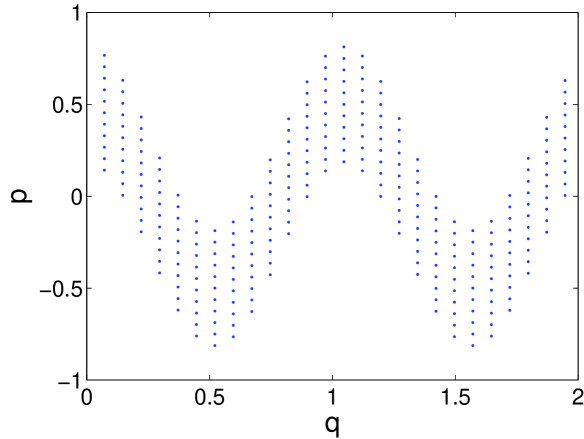
We first give a description of the overall algorithm. To construct the frozen Gaussian approximation on a mesh of 𝒙𝒙\boldsymbol{x}, one needs to compute the integral (2.10) numerically with a mesh of (𝒒,𝒑)𝒒𝒑(\boldsymbol{q},\boldsymbol{p}). This will relate to the numerical computation of (2.11) with a mesh of 𝒚𝒚\boldsymbol{y}. Hence three different meshes are needed in the algorithm. Moreover, the stationary phase approximation implies that ψ±subscript𝜓plus-or-minus\psi_{\pm} in (2.11) is localized around the submanifold 𝒑=𝒒S0(𝒒)𝒑subscript𝒒subscript𝑆0𝒒\boldsymbol{p}=\nabla_{\boldsymbol{q}}S_{0}(\boldsymbol{q}) on phase plane for WKB initial conditions (1.2) when ε𝜀\varepsilon is small. This means we only need to put the mesh grids of 𝒑𝒑\boldsymbol{p} around 𝒒S0(𝒒)subscript𝒒subscript𝑆0𝒒\nabla_{\boldsymbol{q}}S_{0}(\boldsymbol{q}) initially to get a good approximation of the initial value. A one-dimensional example is given to illustrate this localization property of ψ±subscript𝜓plus-or-minus\psi_{\pm} in Figure 1 (left). The associated mesh grids are shown in Figure 1 (right).

Refer to caption
Refer to caption
Figure 1. Left: an illustration of the localization of ψ+subscript𝜓\psi_{+} on (q,p)𝑞𝑝(q,p) domain for u+,0(y)=exp(ısin(6y)12ε)subscript𝑢0𝑦italic-ı6𝑦12𝜀u_{+,0}(y)=\exp\left(\imath\frac{\sin(6y)}{12\varepsilon}\right), ε=1/128𝜀1128\varepsilon=1/128; the black solid curve is p=cos(6q)/2𝑝6𝑞2p=\cos(6q)/2. Right: the corresponding mesh grids of (q,p)𝑞𝑝(q,p).

Next we describe in details all the meshes used in the algorithm.

  1. (1)

    Discrete mesh of (𝒒,𝒑)𝒒𝒑(\boldsymbol{q},\boldsymbol{p}) for initializing 𝑸,𝑷𝑸𝑷\boldsymbol{Q},\boldsymbol{P}. Denote 𝜹𝒒=(δq1,,δqd)𝜹𝒒𝛿subscript𝑞1𝛿subscript𝑞𝑑\boldsymbol{\delta q}=(\delta q_{1},\cdots,\delta q_{d}) and 𝜹𝒑=(δp1,,δpd)𝜹𝒑𝛿subscript𝑝1𝛿subscript𝑝𝑑\boldsymbol{\delta p}=(\delta p_{1},\cdots,\delta p_{d}) as the mesh size. Suppose 𝒒0=(q10,,qd0)superscript𝒒0subscriptsuperscript𝑞01subscriptsuperscript𝑞0𝑑\boldsymbol{q}^{0}=(q^{0}_{1},\cdots,q^{0}_{d}) is the starting point, then the mesh grids 𝒒𝒌superscript𝒒𝒌\boldsymbol{q^{k}}, 𝒌=(k1,,kd)𝒌subscript𝑘1subscript𝑘𝑑\boldsymbol{k}=(k_{1},\cdots,k_{d}), are defined as

    𝒒𝒌=(q10+(k11)δq1,,qd0+(kd1)δqd),superscript𝒒𝒌subscriptsuperscript𝑞01subscript𝑘11𝛿subscript𝑞1subscriptsuperscript𝑞0𝑑subscript𝑘𝑑1𝛿subscript𝑞𝑑\boldsymbol{q^{k}}=\bigl{(}q^{0}_{1}+(k_{1}-1)\delta q_{1},\cdots,q^{0}_{d}+(k_{d}-1)\delta q_{d}\bigr{)},

    where kj=1,,Nqsubscript𝑘𝑗1subscript𝑁𝑞k_{j}=1,\cdots,N_{q} for each j{1,,d}𝑗1𝑑j\in\{1,\cdots,d\}.

    The mesh grids 𝒑𝒌,superscript𝒑𝒌bold-ℓ\boldsymbol{p^{k,\ell}}, =(1,,d)bold-ℓsubscript1subscript𝑑\boldsymbol{\ell}=(\ell_{1},\cdots,\ell_{d}), are defined associated with the mesh grids 𝒒𝒌superscript𝒒𝒌\boldsymbol{q^{k}},

    𝒑𝒌,=(q1S0(𝒒𝒌)+1δp1,,qdS0(𝒒𝒌)+dδpd),superscript𝒑𝒌bold-ℓsubscriptsubscript𝑞1subscript𝑆0superscript𝒒𝒌subscript1𝛿subscript𝑝1subscriptsubscript𝑞𝑑subscript𝑆0superscript𝒒𝒌subscript𝑑𝛿subscript𝑝𝑑\boldsymbol{p^{k,\ell}}=\bigl{(}\partial_{q_{1}}S_{0}(\boldsymbol{q^{k}})+\ell_{1}\delta p_{1},\cdots,\partial_{q_{d}}S_{0}(\boldsymbol{q^{k}})+\ell_{d}\delta p_{d}\bigr{)},

    where j=Np,,Npsubscript𝑗subscript𝑁𝑝subscript𝑁𝑝\ell_{j}=-N_{p},\cdots,N_{p} for each j{1,,d}𝑗1𝑑j\in\{1,\cdots,d\}.

  2. (2)

    Discrete mesh of 𝒚𝒚\boldsymbol{y} for evaluating ψ±subscript𝜓plus-or-minus\psi_{\pm} in (2.11). 𝜹𝒚=(δy1,,δyd)𝜹𝒚𝛿subscript𝑦1𝛿subscript𝑦𝑑\boldsymbol{\delta y}=(\delta y_{1},\cdots,\delta y_{d}) is the mesh size. Denote 𝒚0=(y10,,yd0)superscript𝒚0subscriptsuperscript𝑦01subscriptsuperscript𝑦0𝑑\boldsymbol{y}^{0}=(y^{0}_{1},\cdots,y^{0}_{d}) as the starting point. The mesh grids 𝒚𝒎superscript𝒚𝒎\boldsymbol{y^{m}} are, 𝒎=(m1,,md)𝒎subscript𝑚1subscript𝑚𝑑\boldsymbol{m}=(m_{1},\cdots,m_{d}),

    𝒚𝒎=(y10+(m11)δy1,,yd0+(md1)δyd),superscript𝒚𝒎subscriptsuperscript𝑦01subscript𝑚11𝛿subscript𝑦1subscriptsuperscript𝑦0𝑑subscript𝑚𝑑1𝛿subscript𝑦𝑑\boldsymbol{y^{m}}=\bigl{(}y^{0}_{1}+(m_{1}-1)\delta y_{1},\cdots,y^{0}_{d}+(m_{d}-1)\delta y_{d}\bigr{)},

    where mj=1,,Nysubscript𝑚𝑗1subscript𝑁𝑦m_{j}=1,\cdots,N_{y} for each j{1,,d}𝑗1𝑑j\in\{1,\cdots,d\}.

  3. (3)

    Discrete mesh of 𝒙𝒙\boldsymbol{x} for reconstructing the final solution. 𝜹𝒙=(δx1,,δxd)𝜹𝒙𝛿subscript𝑥1𝛿subscript𝑥𝑑\boldsymbol{\delta x}=(\delta x_{1},\cdots,\delta x_{d}) is the mesh size. Denote 𝒙0=(x10,,xd0)superscript𝒙0subscriptsuperscript𝑥01subscriptsuperscript𝑥0𝑑\boldsymbol{x}^{0}=(x^{0}_{1},\cdots,x^{0}_{d}) as the starting point. The mesh grids 𝒙𝒏superscript𝒙𝒏\boldsymbol{x^{n}} are, 𝒏=(n1,,nd)𝒏subscript𝑛1subscript𝑛𝑑\boldsymbol{n}=(n_{1},\cdots,n_{d}),

    𝒙𝒏=(x10+(n11)δx1,,xd0+(nd1)δxd),superscript𝒙𝒏subscriptsuperscript𝑥01subscript𝑛11𝛿subscript𝑥1subscriptsuperscript𝑥0𝑑subscript𝑛𝑑1𝛿subscript𝑥𝑑\boldsymbol{x^{n}}=\bigl{(}x^{0}_{1}+(n_{1}-1)\delta x_{1},\cdots,x^{0}_{d}+(n_{d}-1)\delta x_{d}\bigr{)},

    where nj=1,,Nxsubscript𝑛𝑗1subscript𝑁𝑥n_{j}=1,\cdots,N_{x} for each j{1,,d}𝑗1𝑑j\in\{1,\cdots,d\}.

With the preparation of the meshes, we introduce the algorithm as follows.

  • Step 1.

    Decompose the initial conditions (1.2) into two branches of waves according to (2.2).

  • Step 2.

    Compute the weight function ψ±subscript𝜓plus-or-minus\psi_{\pm} by (2.11) for (𝑸,𝑷)𝑸𝑷(\boldsymbol{Q},\boldsymbol{P}) initialized at (𝒒𝒌,𝒑𝒌,)superscript𝒒𝒌superscript𝒑𝒌bold-ℓ(\boldsymbol{q^{k}},\boldsymbol{p^{k,\ell}}),

    (2.12) ψ±(𝒒𝒌,𝒑𝒌,)=𝒎eıε(𝒑𝒌,(𝒚𝒎𝒒𝒌)+ı2|𝒚𝒎𝒒𝒌|2)×u±,0(𝒚𝒎)rθ(|𝒚𝒎𝒒𝒌|)δy1δyd,subscript𝜓plus-or-minussuperscript𝒒𝒌superscript𝒑𝒌bold-ℓsubscript𝒎superscript𝑒italic-ı𝜀superscript𝒑𝒌bold-ℓsuperscript𝒚𝒎superscript𝒒𝒌italic-ı2superscriptsuperscript𝒚𝒎superscript𝒒𝒌2subscript𝑢plus-or-minus0superscript𝒚𝒎subscript𝑟𝜃superscript𝒚𝒎superscript𝒒𝒌𝛿subscript𝑦1𝛿subscript𝑦𝑑\psi_{\pm}(\boldsymbol{q^{k}},\boldsymbol{p^{k,\ell}})=\sum_{\boldsymbol{m}}e^{\frac{\imath}{\varepsilon}(-\boldsymbol{p^{k,\ell}}\cdot(\boldsymbol{y^{m}}-\boldsymbol{q^{k}})+\frac{\imath}{2}\lvert\boldsymbol{y^{m}}-\boldsymbol{q^{k}}\rvert^{2})}\\ \times u_{\pm,0}(\boldsymbol{y^{m}})r_{\theta}(\lvert\boldsymbol{y^{m}}-\boldsymbol{q^{k}}\rvert)\delta y_{1}\cdots\delta y_{d},

    where rθsubscript𝑟𝜃r_{\theta} is a cutoff function such that rθ=1subscript𝑟𝜃1r_{\theta}=1 in the ball of radius θ>0𝜃0\theta>0 centered at origin and rθ=0subscript𝑟𝜃0r_{\theta}=0 outside the ball.

  • Step 3.

    Solve (2.4)-(2.5) with the initial conditions

    𝑸±(0,𝒒𝒌,𝒑𝒌,)=𝒒𝒌,𝑷±(0,𝒒𝒌,𝒑𝒌,)=𝒑𝒌,,formulae-sequencesubscript𝑸plus-or-minus0superscript𝒒𝒌superscript𝒑𝒌bold-ℓsuperscript𝒒𝒌subscript𝑷plus-or-minus0superscript𝒒𝒌superscript𝒑𝒌bold-ℓsuperscript𝒑𝒌bold-ℓ\displaystyle\boldsymbol{Q}_{\pm}(0,\boldsymbol{q^{k}},\boldsymbol{p^{k,\ell}})=\boldsymbol{q^{k}},\qquad\boldsymbol{P}_{\pm}(0,\boldsymbol{q^{k}},\boldsymbol{p^{k,\ell}})=\boldsymbol{p^{k,\ell}},
    a±(0,𝒒𝒌,𝒑𝒌,)=2d/2,subscript𝑎plus-or-minus0superscript𝒒𝒌superscript𝒑𝒌bold-ℓsuperscript2𝑑2\displaystyle a_{\pm}(0,\boldsymbol{q^{k}},\boldsymbol{p^{k,\ell}})=2^{d/2},

    by standard numerical integrator for ODE, for example the fourth-order Runge-Kutta scheme. Denote the numerical solutions as (𝑸±𝒌,,𝑷±𝒌,)superscriptsubscript𝑸plus-or-minus𝒌bold-ℓsuperscriptsubscript𝑷plus-or-minus𝒌bold-ℓ(\boldsymbol{Q}_{\pm}^{\boldsymbol{k,\ell}},\boldsymbol{P}_{\pm}^{\boldsymbol{k,\ell}}) and a±𝒌,superscriptsubscript𝑎plus-or-minus𝒌bold-ℓa_{\pm}^{\boldsymbol{k,\ell}}.

  • Step 4.

    Reconstruct the solution by (2.10),

    (2.13) uFGA(t,𝒙𝒏)superscript𝑢FGA𝑡superscript𝒙𝒏\displaystyle u^{\mathrm{FGA}}(t,\boldsymbol{x^{n}}) =𝒌,(a+𝒌,rθ+(2πε)3d/2ψ+(𝒒𝒌,𝒑𝒌,)eıε𝑷+𝒌,(𝒙𝒏𝑸+𝒌,)12ε|𝒙𝒏𝑸+𝒌,|2\displaystyle=\sum_{\boldsymbol{k,\ell}}\biggl{(}\frac{a_{+}^{\boldsymbol{k,\ell}}r_{\theta}^{+}}{(2\pi\varepsilon)^{3d/2}}\psi_{+}(\boldsymbol{q^{k}},\boldsymbol{p^{k,\ell}})e^{\frac{\imath}{\varepsilon}\boldsymbol{P}^{\boldsymbol{k,\ell}}_{+}\cdot(\boldsymbol{x}^{\boldsymbol{n}}-\boldsymbol{Q}^{\boldsymbol{k,\ell}}_{+})-\frac{1}{2\varepsilon}\lvert\boldsymbol{x}^{\boldsymbol{n}}-\boldsymbol{Q}^{\boldsymbol{k,\ell}}_{+}\rvert^{2}}
    +a𝒌,rθ(2πε)3d/2ψ(𝒒𝒌,𝒑𝒌,)eıε𝑷𝒌,(𝒙𝒏𝑸𝒌,)12ε|𝒙𝒏𝑸𝒌,|2)\displaystyle\qquad+\frac{a_{-}^{\boldsymbol{k,\ell}}r_{\theta}^{-}}{(2\pi\varepsilon)^{3d/2}}\psi_{-}(\boldsymbol{q^{k}},\boldsymbol{p^{k,\ell}})e^{\frac{\imath}{\varepsilon}\boldsymbol{P}^{\boldsymbol{k,\ell}}_{-}\cdot(\boldsymbol{x}^{\boldsymbol{n}}-\boldsymbol{Q}^{\boldsymbol{k,\ell}}_{-})-\frac{1}{2\varepsilon}\lvert\boldsymbol{x}^{\boldsymbol{n}}-\boldsymbol{Q}^{\boldsymbol{k,\ell}}_{-}\rvert^{2}}\biggr{)}
    ×δq1δqdδp1δpd,absent𝛿subscript𝑞1𝛿subscript𝑞𝑑𝛿subscript𝑝1𝛿subscript𝑝𝑑\displaystyle\qquad\times\delta q_{1}\cdots\delta q_{d}\delta p_{1}\cdots\delta p_{d},

    where rθ±=rθ(|𝒙𝒏𝑸±𝒌,|)superscriptsubscript𝑟𝜃plus-or-minussubscript𝑟𝜃superscript𝒙𝒏subscriptsuperscript𝑸𝒌bold-ℓplus-or-minusr_{\theta}^{\pm}=r_{\theta}(\lvert\boldsymbol{x}^{\boldsymbol{n}}-\boldsymbol{Q}^{\boldsymbol{k,\ell}}_{\pm}\rvert).

Remark.

1. In setting up the meshes, we assume that the initial condition (1.2) either has compact support or decays sufficiently fast to zero as 𝒙𝒙\boldsymbol{x}\rightarrow\infty so that we only need finite number of mesh points in physical space.

2. The role of the truncation function rθsubscript𝑟𝜃r_{\theta} is to save computational cost, since although a Gaussian function is not localized, it decays quickly away from the center. In practice we take θ=𝒪(ε)𝜃𝒪𝜀\theta=\mathcal{O}(\sqrt{\varepsilon}), the same order as the width of each Gaussian, when we evaluate (2.12) and (2.13) numerically.

3. There are two types of errors present in the method. The first type comes from the asymptotic approximation to the wave equation. This error can not be reduced unless one includes higher order corrections. The other type is the numerical error which comes from two sources: one is from the ODE numerical integrator; the other is from the discrete approximations of integrals (2.10) and (2.11). It can be reduced by either taking small mesh size and time step or using higher order numerical methods.

4. Note that the assumption that the initial conditions are either compactly supported or decay quickly implies that the values on the boundary are zero (or close to zero). Then (2.12) and (2.13) are the trapezoidal rules to approximate (2.11) and (2.10). Notice that, due to the Gaussian factor, the integrand functions in (2.11) and (2.10) are exponentially small unless 𝒙𝑸𝒙𝑸\boldsymbol{x-Q} and 𝒚𝒒𝒚𝒒\boldsymbol{y-q} are in the order of 𝒪(ε1/2)𝒪superscript𝜀12\mathcal{O}({\varepsilon}^{1/2}), which implies their derivatives with respect to 𝒚,𝒒,𝒑𝒚𝒒𝒑\boldsymbol{y},\;\boldsymbol{q},\;\boldsymbol{p} are of the order 𝒪(ε1/2)𝒪superscript𝜀12\mathcal{O}(\varepsilon^{-1/2}). This suggests 𝜹𝒚,𝜹𝒒,𝜹𝒑𝜹𝒚𝜹𝒒𝜹𝒑\boldsymbol{\delta y},\;\boldsymbol{\delta q},\;\boldsymbol{\delta p} should be taken as the size of 𝒪(ε)𝒪𝜀\mathcal{O}(\sqrt{\varepsilon}). Hence Nysubscript𝑁𝑦N_{y} and Nqsubscript𝑁𝑞N_{q} are of order 𝒪(εd/2)𝒪superscript𝜀𝑑2\mathcal{O}(\varepsilon^{-d/2}). As illustrated in Figure 1, Npsubscript𝑁𝑝N_{p} is usually taken as 𝒪(εminjδpj)𝒪𝜀subscript𝑗𝛿subscript𝑝𝑗\mathcal{O}\left(\frac{\sqrt{\varepsilon}}{\min_{j}\;\delta p_{j}}\right), which is of order 𝒪(1)𝒪1\mathcal{O}(1). Nxsubscript𝑁𝑥N_{x} is not constrained by ε𝜀\varepsilon, and is only determined by how well represented one wants the final solution.

5. Step 222 and 444 can be expedited by making use of the discrete fast Gaussian transform, as in [QiYi:app1, QiYi:app2].

3. Asymptotic derivation

We now derive the formulation shown in Section 2 using asymptotic analysis.

We start with the following ansatz for the wave equation (1.1),

(3.1) u(t,𝒙)𝑢𝑡𝒙\displaystyle u(t,\boldsymbol{x}) =1(2πε)3d/23da+(t,𝒒,𝒑)eıεΦ+(t,𝒙,𝒚,𝒒,𝒑)u+,0(𝒚)d𝒚d𝒑d𝒒absent1superscript2𝜋𝜀3𝑑2subscriptsuperscript3𝑑subscript𝑎𝑡𝒒𝒑superscript𝑒italic-ı𝜀subscriptΦ𝑡𝒙𝒚𝒒𝒑subscript𝑢0𝒚differential-d𝒚differential-d𝒑differential-d𝒒\displaystyle=\frac{1}{(2\pi\varepsilon)^{3d/2}}\int_{\mathbb{R}^{3d}}a_{+}(t,\boldsymbol{q},\boldsymbol{p})e^{\frac{\imath}{\varepsilon}\Phi_{+}(t,\boldsymbol{x},\boldsymbol{y},\boldsymbol{q},\boldsymbol{p})}u_{+,0}(\boldsymbol{y})\,\mathrm{d}\boldsymbol{y}\,\mathrm{d}\boldsymbol{p}\,\mathrm{d}\boldsymbol{q}
+1(2πε)3d/23da(t,𝒒,𝒑)eıεΦ(t,𝒙,𝒚,𝒒,𝒑)u,0(𝒚)d𝒚d𝒑d𝒒,1superscript2𝜋𝜀3𝑑2subscriptsuperscript3𝑑subscript𝑎𝑡𝒒𝒑superscript𝑒italic-ı𝜀subscriptΦ𝑡𝒙𝒚𝒒𝒑subscript𝑢0𝒚differential-d𝒚differential-d𝒑differential-d𝒒\displaystyle+\frac{1}{(2\pi\varepsilon)^{3d/2}}\int_{\mathbb{R}^{3d}}a_{-}(t,\boldsymbol{q},\boldsymbol{p})e^{\frac{\imath}{\varepsilon}\Phi_{-}(t,\boldsymbol{x},\boldsymbol{y},\boldsymbol{q},\boldsymbol{p})}u_{-,0}(\boldsymbol{y})\,\mathrm{d}\boldsymbol{y}\,\mathrm{d}\boldsymbol{p}\,\mathrm{d}\boldsymbol{q},

where Φ±subscriptΦplus-or-minus\Phi_{\pm} are given by

(3.2) Φ±(t,𝒙,𝒚,𝒒,𝒑)=S±(t,𝒒,𝒑)+𝑷±(t,𝒒,𝒑)(𝒙𝑸±(t,𝒒,𝒑))𝒑(𝒚𝒒)+ı2|𝒙𝑸±(t,𝒒,𝒑)|2+ı2|𝒚𝒒|2.subscriptΦplus-or-minus𝑡𝒙𝒚𝒒𝒑subscript𝑆plus-or-minus𝑡𝒒𝒑subscript𝑷plus-or-minus𝑡𝒒𝒑𝒙subscript𝑸plus-or-minus𝑡𝒒𝒑𝒑𝒚𝒒italic-ı2superscript𝒙subscript𝑸plus-or-minus𝑡𝒒𝒑2italic-ı2superscript𝒚𝒒2\Phi_{\pm}(t,\boldsymbol{x},\boldsymbol{y},\boldsymbol{q},\boldsymbol{p})=S_{\pm}(t,\boldsymbol{q},\boldsymbol{p})+\boldsymbol{P}_{\pm}(t,\boldsymbol{q},\boldsymbol{p})\cdot(\boldsymbol{x}-\boldsymbol{Q}_{\pm}(t,\boldsymbol{q},\boldsymbol{p}))-\boldsymbol{p}\cdot(\boldsymbol{y}-\boldsymbol{q})\\ +\frac{\imath}{2}\lvert\boldsymbol{x}-\boldsymbol{Q}_{\pm}(t,\boldsymbol{q},\boldsymbol{p})\rvert^{2}+\frac{\imath}{2}\lvert\boldsymbol{y}-\boldsymbol{q}\rvert^{2}.

The initial conditions are taken as

(3.3) 𝑸±(0,𝒒,𝒑)=𝒒,𝑷±(0,𝒒,𝒑)=𝒑,formulae-sequencesubscript𝑸plus-or-minus0𝒒𝒑𝒒subscript𝑷plus-or-minus0𝒒𝒑𝒑\displaystyle\boldsymbol{Q}_{\pm}(0,\boldsymbol{q},\boldsymbol{p})=\boldsymbol{q},\qquad\boldsymbol{P}_{\pm}(0,\boldsymbol{q},\boldsymbol{p})=\boldsymbol{p},
S±(0,𝒒,𝒑)=0,a±(0,𝒒,𝒑)=2d/2.formulae-sequencesubscript𝑆plus-or-minus0𝒒𝒑0subscript𝑎plus-or-minus0𝒒𝒑superscript2𝑑2\displaystyle S_{\pm}(0,\boldsymbol{q},\boldsymbol{p})=0,\qquad a_{\pm}(0,\boldsymbol{q},\boldsymbol{p})=2^{d/2}.

The subscript ±plus-or-minus\pm indicates the two branches that correspond to two different Hamiltonian,

(3.4) H+(𝑸+,𝑷+)=c(𝑸+)|𝑷+|,H(𝑸,𝑷)=c(𝑸)|𝑷|.formulae-sequencesubscript𝐻subscript𝑸subscript𝑷𝑐subscript𝑸subscript𝑷subscript𝐻subscript𝑸subscript𝑷𝑐subscript𝑸subscript𝑷H_{+}(\boldsymbol{Q_{+}},\boldsymbol{P_{+}})=c(\boldsymbol{Q_{+}})\lvert\boldsymbol{P_{+}}\rvert,\qquad H_{-}(\boldsymbol{Q_{-}},\boldsymbol{P_{-}})=-c(\boldsymbol{Q_{-}})\lvert\boldsymbol{P_{-}}\rvert.

𝑷±subscript𝑷plus-or-minus\boldsymbol{P}_{\pm} and 𝑸±subscript𝑸plus-or-minus\boldsymbol{Q}_{\pm} satisfy the equation of motion given by the Hamiltonian H±subscript𝐻plus-or-minusH_{\pm}

(3.5) {t𝑸±=𝑷±H±=±c𝑷±|𝑷±|,t𝑷±=𝑸±H±=𝑸±c|𝑷±|.casessubscript𝑡subscript𝑸plus-or-minussubscriptsubscript𝑷plus-or-minussubscript𝐻plus-or-minusplus-or-minus𝑐subscript𝑷plus-or-minussubscript𝑷plus-or-minusotherwisesubscript𝑡subscript𝑷plus-or-minussubscriptsubscript𝑸plus-or-minussubscript𝐻plus-or-minusminus-or-plussubscriptsubscript𝑸plus-or-minus𝑐subscript𝑷plus-or-minusotherwise\begin{cases}\displaystyle\partial_{t}\boldsymbol{Q}_{\pm}=\partial_{\boldsymbol{P}_{\pm}}H_{\pm}=\pm c\frac{\boldsymbol{P}_{\pm}}{\lvert\boldsymbol{P}_{\pm}\rvert},\\ \displaystyle\partial_{t}\boldsymbol{P}_{\pm}=-\partial_{\boldsymbol{Q}_{\pm}}H_{\pm}=\mp\partial_{\boldsymbol{Q}_{\pm}}c\lvert\boldsymbol{P}_{\pm}\rvert.\end{cases}

By plugging (3.1) into (1.1), the leading order terms show that the evolution of S±subscript𝑆plus-or-minusS_{\pm} simply satisfies

(3.6) tS±=0.subscript𝑡subscript𝑆plus-or-minus0{\partial_{t}S_{\pm}}=0.

This implies S±(t,𝒒,𝒑)=0subscript𝑆plus-or-minus𝑡𝒒𝒑0S_{\pm}(t,\boldsymbol{q},\boldsymbol{p})=0. Hence we omit the terms S±subscript𝑆plus-or-minusS_{\pm} in Section 2 and later calculations.

Before proceeding further, let us state some lemmas that will be used.

Lemma 3.1.

For uL2(d)𝑢superscript𝐿2superscript𝑑u\in L^{2}(\mathbb{R}^{d}), it holds

(3.7) u(𝒙)=1(2πε)3d/23d2d/2eıεΦ±(0,𝒙,𝒚,𝒒,𝒑)u(𝒚)d𝒚d𝒑d𝒒.𝑢𝒙1superscript2𝜋𝜀3𝑑2subscriptsuperscript3𝑑superscript2𝑑2superscript𝑒italic-ı𝜀subscriptΦplus-or-minus0𝒙𝒚𝒒𝒑𝑢𝒚differential-d𝒚differential-d𝒑differential-d𝒒u(\boldsymbol{x})=\frac{1}{(2\pi\varepsilon)^{3d/2}}\int_{\mathbb{R}^{3d}}2^{d/2}e^{\frac{\imath}{\varepsilon}\Phi_{\pm}(0,\boldsymbol{x},\boldsymbol{y},\boldsymbol{q},\boldsymbol{p})}u(\boldsymbol{y})\,\mathrm{d}\boldsymbol{y}\,\mathrm{d}\boldsymbol{p}\,\mathrm{d}\boldsymbol{q}.
Proof.

By the initial conditions (3.3),

(3.8) Φ±(0,𝒙,𝒚,𝒒,𝒑)=𝒑(𝒙𝒒)𝒑(𝒚𝒒)+ı2|𝒙𝒒|2+ı2|𝒚𝒒|2.subscriptΦplus-or-minus0𝒙𝒚𝒒𝒑𝒑𝒙𝒒𝒑𝒚𝒒italic-ı2superscript𝒙𝒒2italic-ı2superscript𝒚𝒒2\Phi_{\pm}(0,\boldsymbol{x},\boldsymbol{y},\boldsymbol{q},\boldsymbol{p})=\boldsymbol{p}\cdot(\boldsymbol{x}-\boldsymbol{q})-\boldsymbol{p}\cdot(\boldsymbol{y}-\boldsymbol{q})+\frac{\imath}{2}\lvert\boldsymbol{x}-\boldsymbol{q}\rvert^{2}+\frac{\imath}{2}\lvert\boldsymbol{y}-\boldsymbol{q}\rvert^{2}.

Therefore, (3.7) is just the standard wave packet decomposition in disguise (see for example [Fo:89]). ∎

The proof of the following important lemma follows the one of Lemma 333 in [SwRo:09].

Lemma 3.2.

For any vector 𝐚(𝐲,𝐪,𝐩)𝐚𝐲𝐪𝐩\boldsymbol{a}(\boldsymbol{y},\boldsymbol{q},\boldsymbol{p}) and matrix M(𝐲,𝐪,𝐩)𝑀𝐲𝐪𝐩M(\boldsymbol{y},\boldsymbol{q},\boldsymbol{p}) in Schwartz class viewed as functions of (𝐲,𝐪,𝐩)𝐲𝐪𝐩(\boldsymbol{y},\boldsymbol{q},\boldsymbol{p}), we have

(3.9) 𝒂(𝒚,𝒒,𝒑)(𝒙𝑸)εzk(ajZjk1),similar-to𝒂𝒚𝒒𝒑𝒙𝑸𝜀subscriptsubscript𝑧𝑘subscript𝑎𝑗superscriptsubscript𝑍𝑗𝑘1\boldsymbol{a}(\boldsymbol{y},\boldsymbol{q},\boldsymbol{p})\cdot(\boldsymbol{x}-\boldsymbol{Q})\sim-\varepsilon\partial_{z_{k}}(a_{j}Z_{jk}^{-1}),

and

(3.10) (𝒙𝑸)M(𝒚,𝒒,𝒑)(𝒙𝑸)εzlQjMjkZkl1+ε2zm(zl(MjkZkl1)Zjm1),similar-to𝒙𝑸𝑀𝒚𝒒𝒑𝒙𝑸𝜀subscriptsubscript𝑧𝑙subscript𝑄𝑗subscript𝑀𝑗𝑘superscriptsubscript𝑍𝑘𝑙1superscript𝜀2subscriptsubscript𝑧𝑚subscriptsubscript𝑧𝑙subscript𝑀𝑗𝑘superscriptsubscript𝑍𝑘𝑙1superscriptsubscript𝑍𝑗𝑚1(\boldsymbol{x}-\boldsymbol{Q})\cdot M(\boldsymbol{y},\boldsymbol{q},\boldsymbol{p})(\boldsymbol{x}-\boldsymbol{Q})\sim\varepsilon\partial_{z_{l}}Q_{j}M_{jk}Z_{kl}^{-1}+\varepsilon^{2}\partial_{z_{m}}\bigl{(}\partial_{z_{l}}(M_{jk}Z_{kl}^{-1})Z_{jm}^{-1}\bigr{)},

where Einstein’s summation convention has been used.

Moreover, for multi-index α𝛼\alpha that |α|3𝛼3\lvert\alpha\rvert\geq 3,

(3.11) (𝒙𝑸)α𝒪(ε|α|1).similar-tosuperscript𝒙𝑸𝛼𝒪superscript𝜀𝛼1(\boldsymbol{x}-\boldsymbol{Q})^{\alpha}\sim\mathcal{O}(\varepsilon^{\lvert\alpha\rvert-1}).

Here we use the notation fgsimilar-to𝑓𝑔f\sim g to mean that

(3.12) 3dfeıεΦ±d𝒚d𝒑d𝒒=3dgeıεΦ±d𝒚d𝒑d𝒒.subscriptsuperscript3𝑑𝑓superscript𝑒italic-ı𝜀subscriptΦplus-or-minusdifferential-d𝒚differential-d𝒑differential-d𝒒subscriptsuperscript3𝑑𝑔superscript𝑒italic-ı𝜀subscriptΦplus-or-minusdifferential-d𝒚differential-d𝒑differential-d𝒒\int_{\mathbb{R}^{3d}}fe^{\frac{\imath}{\varepsilon}\Phi_{\pm}}\,\mathrm{d}\boldsymbol{y}\,\mathrm{d}\boldsymbol{p}\,\mathrm{d}\boldsymbol{q}=\int_{\mathbb{R}^{3d}}ge^{\frac{\imath}{\varepsilon}\Phi_{\pm}}\,\mathrm{d}\boldsymbol{y}\,\mathrm{d}\boldsymbol{p}\,\mathrm{d}\boldsymbol{q}.
Proof.

Since the proof is exactly the same for the cases of Φ+subscriptΦ\Phi_{+} and ΦsubscriptΦ\Phi_{-}, we omit the subscript ±plus-or-minus\pm for simplicity. As 𝒂𝒂\boldsymbol{a} and M𝑀M are in Schwartz class, all the manipulations below are justified.

Observe that at t=0𝑡0t=0,

(𝒒𝑸)𝑷+𝒑=0,(𝒑𝑸)𝑷=0.formulae-sequencesubscript𝒒𝑸𝑷𝒑0subscript𝒑𝑸𝑷0-(\partial_{\boldsymbol{q}}\boldsymbol{Q})\boldsymbol{P}+\boldsymbol{p}=0,\qquad(\partial_{\boldsymbol{p}}\boldsymbol{Q})\boldsymbol{P}=0.

Using (3.5), we have

t((𝒒𝑸)𝑷+𝒑)subscript𝑡subscript𝒒𝑸𝑷𝒑\displaystyle\partial_{t}\bigl{(}-(\partial_{\boldsymbol{q}}\boldsymbol{Q})\boldsymbol{P}+\boldsymbol{p}\bigr{)} =𝒒(t𝑸)𝑷𝒒𝑸t𝑷absentsubscript𝒒subscript𝑡𝑸𝑷subscript𝒒𝑸subscript𝑡𝑷\displaystyle=-\partial_{\boldsymbol{q}}\left(\partial_{t}\boldsymbol{Q}\right)\boldsymbol{P}-\partial_{\boldsymbol{q}}\boldsymbol{Q}\partial_{t}\boldsymbol{P}
=𝒒(c𝑷|𝑷|)𝑷+𝒒𝑸𝑸c|𝑷|absentsubscript𝒒𝑐𝑷𝑷𝑷subscript𝒒𝑸subscript𝑸𝑐𝑷\displaystyle=-\partial_{\boldsymbol{q}}\left(c\frac{\boldsymbol{P}}{\lvert\boldsymbol{P}\rvert}\right)\boldsymbol{P}+\partial_{\boldsymbol{q}}\boldsymbol{Q}\partial_{\boldsymbol{Q}}c\lvert\boldsymbol{P}\rvert
=0.absent0\displaystyle=0.

Analogously we have t((𝒑𝑸)𝑷)=0subscript𝑡subscript𝒑𝑸𝑷0\displaystyle\partial_{t}\bigl{(}(\partial_{\boldsymbol{p}}\boldsymbol{Q})\boldsymbol{P}\bigr{)}=0. Therefore for all t>0𝑡0t>0,

(𝒒𝑸)𝑷+𝒑=0,(𝒑𝑸)𝑷=0.formulae-sequencesubscript𝒒𝑸𝑷𝒑0subscript𝒑𝑸𝑷0-(\partial_{\boldsymbol{q}}\boldsymbol{Q})\boldsymbol{P}+\boldsymbol{p}=0,\qquad(\partial_{\boldsymbol{p}}\boldsymbol{Q})\boldsymbol{P}=0.

Then straightforward calculations yield

𝒒Φ=(𝒒𝑷ı𝒒𝑸)(𝒙𝑸)ı(𝒚𝒒),subscript𝒒Φsubscript𝒒𝑷italic-ısubscript𝒒𝑸𝒙𝑸italic-ı𝒚𝒒\displaystyle\partial_{\boldsymbol{q}}\Phi=(\partial_{\boldsymbol{q}}\boldsymbol{P}-\imath\partial_{\boldsymbol{q}}\boldsymbol{Q})(\boldsymbol{x}-\boldsymbol{Q})-\imath(\boldsymbol{y}-\boldsymbol{q}),
𝒑Φ=(𝒑𝑷ı𝒑𝑸)(𝒙𝑸)(𝒚𝒒),subscript𝒑Φsubscript𝒑𝑷italic-ısubscript𝒑𝑸𝒙𝑸𝒚𝒒\displaystyle\partial_{\boldsymbol{p}}\Phi=(\partial_{\boldsymbol{p}}\boldsymbol{P}-\imath\partial_{\boldsymbol{p}}\boldsymbol{Q})(\boldsymbol{x}-\boldsymbol{Q})-(\boldsymbol{y}-\boldsymbol{q}),

which implies that

(3.13) ı𝒛Φ=Z(𝒙𝑸),italic-ısubscript𝒛Φ𝑍𝒙𝑸\imath\partial_{\boldsymbol{z}}\Phi=Z(\boldsymbol{x}-\boldsymbol{Q}),

where 𝒛subscript𝒛\partial_{\boldsymbol{z}} and Z𝑍Z are defined in (2.6). Note that, Z𝑍Z can be rewritten as

Z=𝒛(𝑸+ı𝑷)=(ıII)(𝒒𝑸𝒒𝑷𝒑𝑸𝒑𝑷)(ıII),𝑍subscript𝒛𝑸italic-ı𝑷matrixitalic-ı𝐼𝐼matrixsubscript𝒒𝑸subscript𝒒𝑷subscript𝒑𝑸subscript𝒑𝑷matrixitalic-ı𝐼𝐼Z=\partial_{\boldsymbol{z}}(\boldsymbol{Q}+\imath\boldsymbol{P})=\begin{pmatrix}\imath I&I\end{pmatrix}\begin{pmatrix}\partial_{\boldsymbol{q}}\boldsymbol{Q}&\partial_{\boldsymbol{q}}\boldsymbol{P}\\ \partial_{\boldsymbol{p}}\boldsymbol{Q}&\partial_{\boldsymbol{p}}\boldsymbol{P}\end{pmatrix}\begin{pmatrix}-\imath I\\ I\end{pmatrix},

where I𝐼I stands for the d×d𝑑𝑑d\times d identity matrix. Therefore, define

F=(𝒒𝑸𝒒𝑷𝒑𝑸𝒑𝑷),𝐹matrixsubscript𝒒𝑸subscript𝒒𝑷subscript𝒑𝑸subscript𝒑𝑷F=\begin{pmatrix}\partial_{\boldsymbol{q}}\boldsymbol{Q}&\partial_{\boldsymbol{q}}\boldsymbol{P}\\ \partial_{\boldsymbol{p}}\boldsymbol{Q}&\partial_{\boldsymbol{p}}\boldsymbol{P}\end{pmatrix},

then

ZZ𝑍superscript𝑍\displaystyle ZZ^{\ast} =(ıII)F(IıIıII)FT(ıII)absentmatrixitalic-ı𝐼𝐼𝐹matrix𝐼italic-ı𝐼italic-ı𝐼𝐼superscript𝐹Tmatrixitalic-ı𝐼𝐼\displaystyle=\begin{pmatrix}\imath I&I\end{pmatrix}F\begin{pmatrix}I&-\imath I\\ \imath I&I\end{pmatrix}F^{\mathrm{T}}\begin{pmatrix}-\imath I\\ I\end{pmatrix}
=(ıII)FFT(ıII)+(ıII)F(0ıIıI0)FT(ıII)absentmatrixitalic-ı𝐼𝐼𝐹superscript𝐹Tmatrixitalic-ı𝐼𝐼matrixitalic-ı𝐼𝐼𝐹matrix0italic-ı𝐼italic-ı𝐼0superscript𝐹Tmatrixitalic-ı𝐼𝐼\displaystyle=\begin{pmatrix}\imath I&I\end{pmatrix}FF^{\mathrm{T}}\begin{pmatrix}-\imath I\\ I\end{pmatrix}+\begin{pmatrix}\imath I&I\end{pmatrix}F\begin{pmatrix}0&-\imath I\\ \imath I&0\end{pmatrix}F^{\mathrm{T}}\begin{pmatrix}-\imath I\\ I\end{pmatrix}
=(ıII)FFT(ıII)+2I.absentmatrixitalic-ı𝐼𝐼𝐹superscript𝐹Tmatrixitalic-ı𝐼𝐼2𝐼\displaystyle=\begin{pmatrix}\imath I&I\end{pmatrix}FF^{\mathrm{T}}\begin{pmatrix}-\imath I\\ I\end{pmatrix}+2I.

In the last equality, we have used the fact that

F(0ıIıI0)FT=(0ıIıI0),𝐹matrix0italic-ı𝐼italic-ı𝐼0superscript𝐹Tmatrix0italic-ı𝐼italic-ı𝐼0F\begin{pmatrix}0&-\imath I\\ \imath I&0\end{pmatrix}F^{\mathrm{T}}=\begin{pmatrix}0&-\imath I\\ \imath I&0\end{pmatrix},

due to the Hamiltonian flow structure. Therefore ZZ𝑍superscript𝑍ZZ^{\ast} is positive definite for all t𝑡t, which implies Z𝑍Z is invertible and

(3.14) (𝒙𝑸)=ıZ1𝒛Φ.𝒙𝑸italic-ısuperscript𝑍1subscript𝒛Φ(\boldsymbol{x}-\boldsymbol{Q})=\imath Z^{-1}\partial_{\boldsymbol{z}}\Phi.

Using (3.14), one has

3d𝒂(𝒙𝑸)eıεΦd𝒚d𝒑d𝒒subscriptsuperscript3𝑑𝒂𝒙𝑸superscript𝑒italic-ı𝜀Φdifferential-d𝒚differential-d𝒑differential-d𝒒\displaystyle\int_{\mathbb{R}^{3d}}\boldsymbol{a}\cdot(\boldsymbol{x}-\boldsymbol{Q})e^{\frac{\imath}{\varepsilon}\Phi}\,\mathrm{d}\boldsymbol{y}\,\mathrm{d}\boldsymbol{p}\,\mathrm{d}\boldsymbol{q} =ε3dajZjk1(ıεzkΦ)eıεΦd𝒚d𝒑d𝒒absent𝜀subscriptsuperscript3𝑑subscript𝑎𝑗subscriptsuperscript𝑍1𝑗𝑘italic-ı𝜀subscriptsubscript𝑧𝑘Φsuperscript𝑒italic-ı𝜀Φdifferential-d𝒚differential-d𝒑differential-d𝒒\displaystyle=\varepsilon\int_{\mathbb{R}^{3d}}{a}_{j}Z^{-1}_{jk}\left(\frac{\imath}{\varepsilon}\partial_{z_{k}}\Phi\right)e^{\frac{\imath}{\varepsilon}\Phi}\,\mathrm{d}\boldsymbol{y}\,\mathrm{d}\boldsymbol{p}\,\mathrm{d}\boldsymbol{q}
=ε3dzk(ajZjk1)eıεΦd𝒚d𝒑d𝒒,absent𝜀subscriptsuperscript3𝑑subscriptsubscript𝑧𝑘subscript𝑎𝑗subscriptsuperscript𝑍1𝑗𝑘superscript𝑒italic-ı𝜀Φd𝒚d𝒑d𝒒\displaystyle=-\varepsilon\int_{\mathbb{R}^{3d}}\partial_{z_{k}}\big{(}{a}_{j}Z^{-1}_{jk}\big{)}e^{\frac{\imath}{\varepsilon}\Phi}\,\mathrm{d}\boldsymbol{y}\,\mathrm{d}\boldsymbol{p}\,\mathrm{d}\boldsymbol{q},

where the last equality is obtained from integration by parts. This proves (3.9).

Making use of (3.9) twice produces (3.10)

(𝒙𝑸)M(𝒙𝑸)𝒙𝑸𝑀𝒙𝑸\displaystyle(\boldsymbol{x}-\boldsymbol{Q})\cdot M(\boldsymbol{x}-\boldsymbol{Q}) =(xQ)jMjk(xQ)kabsentsubscript𝑥𝑄𝑗subscript𝑀𝑗𝑘subscript𝑥𝑄𝑘\displaystyle=(x-Q)_{j}M_{jk}(x-Q)_{k}
εzl((xQ)jMjkZkl1)similar-toabsent𝜀subscriptsubscript𝑧𝑙subscript𝑥𝑄𝑗subscript𝑀𝑗𝑘subscriptsuperscript𝑍1𝑘𝑙\displaystyle\sim-\varepsilon\partial_{z_{l}}\bigl{(}(x-Q)_{j}M_{jk}Z^{-1}_{kl}\bigr{)}
=εzlQjMjkZkl1ε(xQ)jzl(MjkZkl1)absent𝜀subscriptsubscript𝑧𝑙subscript𝑄𝑗subscript𝑀𝑗𝑘superscriptsubscript𝑍𝑘𝑙1𝜀subscript𝑥𝑄𝑗subscriptsubscript𝑧𝑙subscript𝑀𝑗𝑘subscriptsuperscript𝑍1𝑘𝑙\displaystyle=\varepsilon\partial_{z_{l}}Q_{j}M_{jk}Z_{kl}^{-1}-\varepsilon(x-Q)_{j}\partial_{z_{l}}(M_{jk}Z^{-1}_{kl})
εzlQjMjkZkl1+ε2zm(zl(MjkZkl1)Zjm1).similar-toabsent𝜀subscriptsubscript𝑧𝑙subscript𝑄𝑗subscript𝑀𝑗𝑘superscriptsubscript𝑍𝑘𝑙1superscript𝜀2subscriptsubscript𝑧𝑚subscriptsubscript𝑧𝑙subscript𝑀𝑗𝑘superscriptsubscript𝑍𝑘𝑙1superscriptsubscript𝑍𝑗𝑚1\displaystyle\sim\varepsilon\partial_{z_{l}}Q_{j}M_{jk}Z_{kl}^{-1}+\varepsilon^{2}\partial_{z_{m}}\bigl{(}\partial_{z_{l}}(M_{jk}Z_{kl}^{-1})Z_{jm}^{-1}\bigr{)}.

By induction it is easy to see that (3.11) is true.

3.1. Initial value decomposition

By (3.2) and (3.5) we obtain that

(3.15) tΦ±subscript𝑡subscriptΦplus-or-minus\displaystyle\partial_{t}\Phi_{\pm} =𝑷±t𝑸±+(t𝑷±ıt𝑸±)(𝒙𝑸±)absentsubscript𝑷plus-or-minussubscript𝑡subscript𝑸plus-or-minussubscript𝑡subscript𝑷plus-or-minusitalic-ısubscript𝑡subscript𝑸plus-or-minus𝒙subscript𝑸plus-or-minus\displaystyle=-\boldsymbol{P}_{\pm}\cdot\partial_{t}\boldsymbol{Q}_{\pm}+(\partial_{t}\boldsymbol{P}_{\pm}-\imath\partial_{t}\boldsymbol{Q}_{\pm})\cdot(\boldsymbol{x}-\boldsymbol{Q}_{\pm})
=c|𝑷±|(𝒙𝑸±)(|𝑷±|𝑸±c+ı𝑷±|𝑷±|c),absentminus-or-plusminus-or-plus𝑐subscript𝑷plus-or-minus𝒙subscript𝑸plus-or-minussubscript𝑷plus-or-minussubscriptsubscript𝑸plus-or-minus𝑐italic-ısubscript𝑷plus-or-minussubscript𝑷plus-or-minus𝑐\displaystyle=\mp c\lvert\boldsymbol{P}_{\pm}\rvert\mp(\boldsymbol{x}-\boldsymbol{Q}_{\pm})\cdot\Bigl{(}\lvert\boldsymbol{P}_{\pm}\rvert\partial_{\boldsymbol{Q}_{\pm}}c+\imath\frac{\boldsymbol{P}_{\pm}}{\lvert\boldsymbol{P}_{\pm}\rvert}c\Bigr{)},

and in particular for t=0𝑡0t=0,

(3.16) tΦ±(0,𝒙,𝒚,𝒒,𝒑)=c|𝒑|(𝒙𝒒)(|𝒑|𝒒c+ı𝒑|𝒑|c).subscript𝑡subscriptΦplus-or-minus0𝒙𝒚𝒒𝒑minus-or-plusminus-or-plus𝑐𝒑𝒙𝒒𝒑subscript𝒒𝑐italic-ı𝒑𝒑𝑐\partial_{t}\Phi_{\pm}(0,\boldsymbol{x},\boldsymbol{y},\boldsymbol{q},\boldsymbol{p})=\mp c\lvert\boldsymbol{p}\rvert\mp(\boldsymbol{x}-\boldsymbol{q})\cdot\Bigl{(}\lvert\boldsymbol{p}\rvert\partial_{\boldsymbol{q}}c+\imath\frac{\boldsymbol{p}}{\lvert\boldsymbol{p}\rvert}c\Bigr{)}.

The ansatz (3.1) shows that

(3.17) u(0,𝒙)𝑢0𝒙\displaystyle u(0,\boldsymbol{x}) =1(2πε)3d/23da+(0,𝒒,𝒑)eıεΦ+(0,𝒙,𝒚,𝒒,𝒑)u+,0(𝒚)d𝒚d𝒑d𝒒absent1superscript2𝜋𝜀3𝑑2subscriptsuperscript3𝑑subscript𝑎0𝒒𝒑superscript𝑒italic-ı𝜀subscriptΦ0𝒙𝒚𝒒𝒑subscript𝑢0𝒚differential-d𝒚differential-d𝒑differential-d𝒒\displaystyle=\frac{1}{(2\pi\varepsilon)^{3d/2}}\int_{\mathbb{R}^{3d}}a_{+}(0,\boldsymbol{q},\boldsymbol{p})e^{\frac{\imath}{\varepsilon}\Phi_{+}(0,\boldsymbol{x},\boldsymbol{y},\boldsymbol{q},\boldsymbol{p})}u_{+,0}(\boldsymbol{y})\,\mathrm{d}\boldsymbol{y}\,\mathrm{d}\boldsymbol{p}\,\mathrm{d}\boldsymbol{q}
+1(2πε)3d/23da(0,𝒑,𝒒)eıεΦ(0,𝒙,𝒚,𝒒,𝒑)u,0(𝒚)d𝒚d𝒑d𝒒,1superscript2𝜋𝜀3𝑑2subscriptsuperscript3𝑑subscript𝑎0𝒑𝒒superscript𝑒italic-ı𝜀subscriptΦ0𝒙𝒚𝒒𝒑subscript𝑢0𝒚differential-d𝒚differential-d𝒑differential-d𝒒\displaystyle+\frac{1}{(2\pi\varepsilon)^{3d/2}}\int_{\mathbb{R}^{3d}}a_{-}(0,\boldsymbol{p},\boldsymbol{q})e^{\frac{\imath}{\varepsilon}\Phi_{-}(0,\boldsymbol{x},\boldsymbol{y},\boldsymbol{q},\boldsymbol{p})}u_{-,0}(\boldsymbol{y})\,\mathrm{d}\boldsymbol{y}\,\mathrm{d}\boldsymbol{p}\,\mathrm{d}\boldsymbol{q},

and

(3.18) tu(0,𝒙)subscript𝑡𝑢0𝒙\displaystyle\partial_{t}u(0,\boldsymbol{x}) =1(2πε)3d/23d(ta++ıa+εtΦ+)eıεΦ+(0,𝒙,𝒚,𝒒,𝒑)u+,0(𝒚)d𝒚d𝒑d𝒒absent1superscript2𝜋𝜀3𝑑2subscriptsuperscript3𝑑subscript𝑡subscript𝑎italic-ısubscript𝑎𝜀subscript𝑡subscriptΦsuperscript𝑒italic-ı𝜀subscriptΦ0𝒙𝒚𝒒𝒑subscript𝑢0𝒚differential-d𝒚differential-d𝒑differential-d𝒒\displaystyle=\frac{1}{(2\pi\varepsilon)^{3d/2}}\int_{\mathbb{R}^{3d}}\bigl{(}\partial_{t}a_{+}+\frac{\imath a_{+}}{\varepsilon}\partial_{t}\Phi_{+}\bigr{)}e^{\frac{\imath}{\varepsilon}\Phi_{+}(0,\boldsymbol{x},\boldsymbol{y},\boldsymbol{q},\boldsymbol{p})}u_{+,0}(\boldsymbol{y})\,\mathrm{d}\boldsymbol{y}\,\mathrm{d}\boldsymbol{p}\,\mathrm{d}\boldsymbol{q}
+1(2πε)3d/23d(ta+ıaεtΦ)eıεΦ(0,𝒙,𝒚,𝒒,𝒑)u,0(𝒚)d𝒚d𝒑d𝒒.1superscript2𝜋𝜀3𝑑2subscriptsuperscript3𝑑subscript𝑡subscript𝑎italic-ısubscript𝑎𝜀subscript𝑡subscriptΦsuperscript𝑒italic-ı𝜀subscriptΦ0𝒙𝒚𝒒𝒑subscript𝑢0𝒚differential-d𝒚differential-d𝒑differential-d𝒒\displaystyle+\frac{1}{(2\pi\varepsilon)^{3d/2}}\int_{\mathbb{R}^{3d}}\bigl{(}\partial_{t}a_{-}+\frac{\imath a_{-}}{\varepsilon}\partial_{t}\Phi_{-}\bigr{)}e^{\frac{\imath}{\varepsilon}\Phi_{-}(0,\boldsymbol{x},\boldsymbol{y},\boldsymbol{q},\boldsymbol{p})}u_{-,0}(\boldsymbol{y})\,\mathrm{d}\boldsymbol{y}\,\mathrm{d}\boldsymbol{p}\,\mathrm{d}\boldsymbol{q}.

We take

(3.19) a±(0,𝒒,𝒑)=2d/2,subscript𝑎plus-or-minus0𝒒𝒑superscript2𝑑2\displaystyle a_{\pm}(0,\boldsymbol{q},\boldsymbol{p})=2^{d/2},
(3.20) u+,0(𝒙)=A+(𝒙)eıεS0(𝒙),subscript𝑢0𝒙subscript𝐴𝒙superscript𝑒italic-ı𝜀subscript𝑆0𝒙\displaystyle u_{+,0}(\boldsymbol{x})=A_{+}(\boldsymbol{x})e^{\frac{\imath}{\varepsilon}S_{0}(\boldsymbol{x})},
(3.21) u,0(𝒙)=A(𝒙)eıεS0(𝒙),subscript𝑢0𝒙subscript𝐴𝒙superscript𝑒italic-ı𝜀subscript𝑆0𝒙\displaystyle u_{-,0}(\boldsymbol{x})=A_{-}(\boldsymbol{x})e^{\frac{\imath}{\varepsilon}S_{0}(\boldsymbol{x})},

with

(3.22) A±(𝒙)=12(A0(𝒙)±ıB0(𝒙)c(𝒙)|𝒙S0(𝒙)|).subscript𝐴plus-or-minus𝒙12plus-or-minussubscript𝐴0𝒙italic-ısubscript𝐵0𝒙𝑐𝒙subscript𝒙subscript𝑆0𝒙A_{\pm}(\boldsymbol{x})=\frac{1}{2}\biggl{(}A_{0}(\boldsymbol{x})\pm\frac{\imath B_{0}(\boldsymbol{x})}{c(\boldsymbol{x})\lvert\partial_{\boldsymbol{x}}S_{0}(\boldsymbol{x})\rvert}\biggr{)}.

We next show that this will approximate the initial condition to the leading order in ε𝜀\varepsilon.

Substituting (3.19)-(3.22) into (3.17) and using Lemma 3.1, we easily confirm that

u(0,𝒙)=u+,0(𝒙)+u,0(𝒙)=A0(𝒙)eıεS0(𝒙).𝑢0𝒙subscript𝑢0𝒙subscript𝑢0𝒙subscript𝐴0𝒙superscript𝑒italic-ı𝜀subscript𝑆0𝒙u(0,\boldsymbol{x})=u_{+,0}(\boldsymbol{x})+u_{-,0}(\boldsymbol{x})=A_{0}(\boldsymbol{x})e^{\frac{\imath}{\varepsilon}S_{0}(\boldsymbol{x})}.

For the initial velocity, we substitute (3.19)-(3.22) into (3.18) and keep only the leading order terms in ε𝜀\varepsilon. According to Lemma 3.2, only the term c|𝒑|minus-or-plus𝑐𝒑\mp c\lvert\boldsymbol{p}\rvert in tΦ±subscript𝑡subscriptΦplus-or-minus\partial_{t}\Phi_{\pm} will contribute to the leading order, since the other terms that contain (𝒙𝒒)𝒙𝒒(\boldsymbol{x}-\boldsymbol{q}) are 𝒪(ε)𝒪𝜀\mathcal{O}(\varepsilon). Hence,

tu(0,𝒙)=subscript𝑡𝑢0𝒙absent\displaystyle\partial_{t}u(0,\boldsymbol{x})= 2d/2(2πε)3d/23dıεc(𝒒)|𝒑|eıεΦ+(0,𝒙,𝒚,𝒒,𝒑)u+,0(𝒚)d𝒚d𝒑d𝒒superscript2𝑑2superscript2𝜋𝜀3𝑑2subscriptsuperscript3𝑑italic-ı𝜀𝑐𝒒𝒑superscript𝑒italic-ı𝜀subscriptΦ0𝒙𝒚𝒒𝒑subscript𝑢0𝒚differential-d𝒚differential-d𝒑differential-d𝒒\displaystyle-\frac{2^{d/2}}{(2\pi\varepsilon)^{3d/2}}\int_{\mathbb{R}^{3d}}\frac{\imath}{\varepsilon}c(\boldsymbol{q})\lvert\boldsymbol{p}\rvert e^{\frac{\imath}{\varepsilon}\Phi_{+}(0,\boldsymbol{x},\boldsymbol{y},\boldsymbol{q},\boldsymbol{p})}u_{+,0}(\boldsymbol{y})\,\mathrm{d}\boldsymbol{y}\,\mathrm{d}\boldsymbol{p}\,\mathrm{d}\boldsymbol{q}
+2d/2(2πε)3d/23dıεc(𝒒)|𝒑|eıεΦ(0,𝒙,𝒚,𝒒,𝒑)u,0(𝒚)d𝒚d𝒑d𝒒+𝒪(1).superscript2𝑑2superscript2𝜋𝜀3𝑑2subscriptsuperscript3𝑑italic-ı𝜀𝑐𝒒𝒑superscript𝑒italic-ı𝜀subscriptΦ0𝒙𝒚𝒒𝒑subscript𝑢0𝒚differential-d𝒚differential-d𝒑differential-d𝒒𝒪1\displaystyle+\frac{2^{d/2}}{(2\pi\varepsilon)^{3d/2}}\int_{\mathbb{R}^{3d}}\frac{\imath}{\varepsilon}c(\boldsymbol{q})\lvert\boldsymbol{p}\rvert e^{\frac{\imath}{\varepsilon}\Phi_{-}(0,\boldsymbol{x},\boldsymbol{y},\boldsymbol{q},\boldsymbol{p})}u_{-,0}(\boldsymbol{y})\,\mathrm{d}\boldsymbol{y}\,\mathrm{d}\boldsymbol{p}\,\mathrm{d}\boldsymbol{q}+\mathcal{O}(1).

Consider the integral

dc(𝒒)|𝒑|eıε𝒑(𝒚𝒒)12ε|𝒚𝒒|2A±(𝒚)eıεS0(𝒚)d𝒚=dc(𝒒)|𝒑|A±(𝒚)eıεΘ(𝒚,𝒒,𝒑)d𝒚.subscriptsuperscript𝑑𝑐𝒒𝒑superscript𝑒italic-ı𝜀𝒑𝒚𝒒12𝜀superscript𝒚𝒒2subscript𝐴plus-or-minus𝒚superscript𝑒italic-ı𝜀subscript𝑆0𝒚differential-d𝒚subscriptsuperscript𝑑𝑐𝒒𝒑subscript𝐴plus-or-minus𝒚superscript𝑒italic-ı𝜀Θ𝒚𝒒𝒑differential-d𝒚\int_{\mathbb{R}^{d}}c(\boldsymbol{q})\lvert\boldsymbol{p}\rvert e^{-\frac{\imath}{\varepsilon}\boldsymbol{p}\cdot(\boldsymbol{y}-\boldsymbol{q})-\frac{1}{2\varepsilon}\lvert\boldsymbol{y}-\boldsymbol{q}\rvert^{2}}A_{\pm}(\boldsymbol{y})e^{\frac{\imath}{\varepsilon}S_{0}(\boldsymbol{y})}\,\mathrm{d}\boldsymbol{y}=\int_{\mathbb{R}^{d}}c(\boldsymbol{q})\lvert\boldsymbol{p}\rvert A_{\pm}(\boldsymbol{y})e^{\frac{\imath}{\varepsilon}\Theta(\boldsymbol{y},\boldsymbol{q},\boldsymbol{p})}\,\mathrm{d}\boldsymbol{y}.

The phase function ΘΘ\Theta is given by

Θ(𝒚,𝒒,𝒑)=𝒑(𝒚𝒒)+ı2|𝒚𝒒|2+S0(𝒚).Θ𝒚𝒒𝒑𝒑𝒚𝒒italic-ı2superscript𝒚𝒒2subscript𝑆0𝒚\Theta(\boldsymbol{y},\boldsymbol{q},\boldsymbol{p})=-\boldsymbol{p}\cdot(\boldsymbol{y}-\boldsymbol{q})+\frac{\imath}{2}\lvert\boldsymbol{y}-\boldsymbol{q}\rvert^{2}+S_{0}(\boldsymbol{y}).

Clearly, 𝔪Θ0𝔪Θ0\mathfrak{Im}\;\Theta\geq 0 and 𝔪Θ=0𝔪Θ0\mathfrak{Im}\;\Theta=0 if and only if 𝒚=𝒒𝒚𝒒\boldsymbol{y}=\boldsymbol{q}. The derivatives of ΘΘ\Theta with respect to 𝒚𝒚\boldsymbol{y} are

𝒚Θ=𝒑+𝒚S0(𝒚)+ı(𝒚𝒒),subscript𝒚Θ𝒑subscript𝒚subscript𝑆0𝒚italic-ı𝒚𝒒\displaystyle\partial_{\boldsymbol{y}}\Theta=-\boldsymbol{p}+\partial_{\boldsymbol{y}}S_{0}(\boldsymbol{y})+\imath(\boldsymbol{y}-\boldsymbol{q}),
𝒚2Θ=𝒚2S0(𝒚)+iI.superscriptsubscript𝒚2Θsuperscriptsubscript𝒚2subscript𝑆0𝒚𝑖𝐼\displaystyle\partial_{\boldsymbol{y}}^{2}\Theta=\partial_{\boldsymbol{y}}^{2}S_{0}(\boldsymbol{y})+iI.

Hence, the first derivative vanishes only when 𝒚=𝒒𝒚𝒒\boldsymbol{y}=\boldsymbol{q} and 𝒑=𝒚S0(𝒚)𝒑subscript𝒚subscript𝑆0𝒚\boldsymbol{p}=\partial_{\boldsymbol{y}}S_{0}(\boldsymbol{y}), and det𝒚2Θ0superscriptsubscript𝒚2Θ0\det\partial_{\boldsymbol{y}}^{2}\Theta\not=0. Therefore, we can apply stationary phase approximation with complex phase (see for example [Ho:83]) to conclude, for (𝒒,𝒑)2d𝒒𝒑superscript2𝑑(\boldsymbol{q},\boldsymbol{p})\in\mathbb{R}^{2d},

dc(𝒒)|𝒑|eıε𝒑(𝒚𝒒)12ε|𝒚𝒒|2A±(𝒚)eıεS0(𝒚)d𝒚=dc(𝒚)|𝒚S0(𝒚)|eıε𝒑(𝒚𝒒)12ε|𝒚𝒒|2A±(𝒚)eıεS0(𝒚)d𝒚+𝒪(ε).subscriptsuperscript𝑑𝑐𝒒𝒑superscript𝑒italic-ı𝜀𝒑𝒚𝒒12𝜀superscript𝒚𝒒2subscript𝐴plus-or-minus𝒚superscript𝑒italic-ı𝜀subscript𝑆0𝒚differential-d𝒚subscriptsuperscript𝑑𝑐𝒚subscript𝒚subscript𝑆0𝒚superscript𝑒italic-ı𝜀𝒑𝒚𝒒12𝜀superscript𝒚𝒒2subscript𝐴plus-or-minus𝒚superscript𝑒italic-ı𝜀subscript𝑆0𝒚differential-d𝒚𝒪𝜀\int_{\mathbb{R}^{d}}c(\boldsymbol{q})\lvert\boldsymbol{p}\rvert e^{-\frac{\imath}{\varepsilon}\boldsymbol{p}\cdot(\boldsymbol{y}-\boldsymbol{q})-\frac{1}{2\varepsilon}\lvert\boldsymbol{y}-\boldsymbol{q}\rvert^{2}}A_{\pm}(\boldsymbol{y})e^{\frac{\imath}{\varepsilon}S_{0}(\boldsymbol{y})}\,\mathrm{d}\boldsymbol{y}\\ =\int_{\mathbb{R}^{d}}c(\boldsymbol{y})\lvert\partial_{\boldsymbol{y}}S_{0}(\boldsymbol{y})\rvert e^{-\frac{\imath}{\varepsilon}\boldsymbol{p}\cdot(\boldsymbol{y}-\boldsymbol{q})-\frac{1}{2\varepsilon}\lvert\boldsymbol{y}-\boldsymbol{q}\rvert^{2}}A_{\pm}(\boldsymbol{y})e^{\frac{\imath}{\varepsilon}S_{0}(\boldsymbol{y})}\,\mathrm{d}\boldsymbol{y}+\mathcal{O}(\varepsilon).

Therefore,

(3.23) tu(0,𝒙)=2d/2(2πε)3d/23dıεc(𝒚)|𝒚S0(𝒚)|eıεΦ+(0,𝒙,𝒚,𝒒,𝒑)u+,0(𝒚)d𝒚d𝒑d𝒒+2d/2(2πε)3d/23dıεc(𝒚)|𝒚S0(𝒚)|eıεΦ(0,𝒙,𝒚,𝒒,𝒑)u,0(𝒚)d𝒚d𝒑d𝒒+𝒪(1).subscript𝑡𝑢0𝒙superscript2𝑑2superscript2𝜋𝜀3𝑑2subscriptsuperscript3𝑑italic-ı𝜀𝑐𝒚subscript𝒚subscript𝑆0𝒚superscript𝑒italic-ı𝜀subscriptΦ0𝒙𝒚𝒒𝒑subscript𝑢0𝒚differential-d𝒚differential-d𝒑differential-d𝒒superscript2𝑑2superscript2𝜋𝜀3𝑑2subscriptsuperscript3𝑑italic-ı𝜀𝑐𝒚subscript𝒚subscript𝑆0𝒚superscript𝑒italic-ı𝜀subscriptΦ0𝒙𝒚𝒒𝒑subscript𝑢0𝒚differential-d𝒚differential-d𝒑differential-d𝒒𝒪1\partial_{t}u(0,\boldsymbol{x})=-\frac{2^{d/2}}{(2\pi\varepsilon)^{3d/2}}\int_{\mathbb{R}^{3d}}\frac{\imath}{\varepsilon}c(\boldsymbol{y})\lvert\partial_{\boldsymbol{y}}S_{0}(\boldsymbol{y})\rvert e^{\frac{\imath}{\varepsilon}\Phi_{+}(0,\boldsymbol{x},\boldsymbol{y},\boldsymbol{q},\boldsymbol{p})}u_{+,0}(\boldsymbol{y})\,\mathrm{d}\boldsymbol{y}\,\mathrm{d}\boldsymbol{p}\,\mathrm{d}\boldsymbol{q}\\ +\frac{2^{d/2}}{(2\pi\varepsilon)^{3d/2}}\int_{\mathbb{R}^{3d}}\frac{\imath}{\varepsilon}c(\boldsymbol{y})\lvert\partial_{\boldsymbol{y}}S_{0}(\boldsymbol{y})\rvert e^{\frac{\imath}{\varepsilon}\Phi_{-}(0,\boldsymbol{x},\boldsymbol{y},\boldsymbol{q},\boldsymbol{p})}u_{-,0}(\boldsymbol{y})\,\mathrm{d}\boldsymbol{y}\,\mathrm{d}\boldsymbol{p}\,\mathrm{d}\boldsymbol{q}+\mathcal{O}(1).

Substitute (3.22) into (3.23) and use Lemma 3.1, then

tu(0,𝒙)=1εB0(𝒙)eıεS0(𝒙),subscript𝑡𝑢0𝒙1𝜀subscript𝐵0𝒙superscript𝑒italic-ı𝜀subscript𝑆0𝒙\partial_{t}u(0,\boldsymbol{x})=\frac{1}{\varepsilon}B_{0}(\boldsymbol{x})e^{\frac{\imath}{\varepsilon}S_{0}(\boldsymbol{x})},

which agrees with (1.2).

3.2. Derivation of the evolution equation of a±subscript𝑎plus-or-minusa_{\pm}

In order to derive the evolution equation for the weight function a𝑎a, we carry out the asymptotic analysis of the wave equation (1.1) using the ansatz (3.1) in this section. As the equation (1.1) is linear, we can deal with the two branches separately. In the following, we only deal with the “++” branch that corresponds to H+subscript𝐻H_{+}, and the other is completely analogous. For simplicity, we drop the subscript “++” in the notations.

Substituting (3.1) into the equation (1.1) (keeping only the “++” branch) gives

t2u=1(2πε)3d/23d(t2a+2ıεtatΦ+ıεat2Φ1ε2a(tΦ)2)eıΦ/εu0d𝒚d𝒑d𝒒,superscriptsubscript𝑡2𝑢1superscript2𝜋𝜀3𝑑2subscriptsuperscript3𝑑superscriptsubscript𝑡2𝑎2italic-ı𝜀subscript𝑡𝑎subscript𝑡Φitalic-ı𝜀𝑎superscriptsubscript𝑡2Φ1superscript𝜀2𝑎superscriptsubscript𝑡Φ2superscript𝑒italic-ıΦ𝜀subscript𝑢0differential-d𝒚differential-d𝒑differential-d𝒒\partial_{t}^{2}u=\frac{1}{(2\pi\varepsilon)^{3d/2}}\int_{\mathbb{R}^{3d}}\Bigl{(}\partial_{t}^{2}a+2\frac{\imath}{\varepsilon}\partial_{t}a\partial_{t}\Phi+\frac{\imath}{\varepsilon}a\partial_{t}^{2}\Phi-\frac{1}{\varepsilon^{2}}a(\partial_{t}\Phi)^{2}\Bigr{)}e^{\imath\Phi/\varepsilon}u_{0}\,\mathrm{d}\boldsymbol{y}\,\mathrm{d}\boldsymbol{p}\,\mathrm{d}\boldsymbol{q},

and

Δu=1(2πε)3d/23d(ıεΔΦ1ε2(𝒙Φ𝒙Φ))aeıΦ/εu0d𝒚d𝒑d𝒒.Δ𝑢1superscript2𝜋𝜀3𝑑2subscriptsuperscript3𝑑italic-ı𝜀ΔΦ1superscript𝜀2subscript𝒙Φsubscript𝒙Φ𝑎superscript𝑒italic-ıΦ𝜀subscript𝑢0differential-d𝒚differential-d𝒑differential-d𝒒\Delta u=\frac{1}{(2\pi\varepsilon)^{3d/2}}\int_{\mathbb{R}^{3d}}\Bigl{(}\frac{\imath}{\varepsilon}\Delta\Phi-\frac{1}{\varepsilon^{2}}(\partial_{\boldsymbol{x}}\Phi\cdot\partial_{\boldsymbol{x}}\Phi)\Bigr{)}ae^{\imath\Phi/\varepsilon}u_{0}\,\mathrm{d}\boldsymbol{y}\,\mathrm{d}\boldsymbol{p}\,\mathrm{d}\boldsymbol{q}.

Squaring both sides of (3.15) yields

(3.24) (tΦ)2=c2|𝑷|2+((𝒙𝑸)(|𝑷|𝑸c+ıc𝑷|𝑷|))2+2c|𝑷|(𝒙𝑸)(|𝑷|𝑸c+ıc𝑷|𝑷|).superscriptsubscript𝑡Φ2superscript𝑐2superscript𝑷2superscript𝒙𝑸𝑷subscript𝑸𝑐italic-ı𝑐𝑷𝑷22𝑐𝑷𝒙𝑸𝑷subscript𝑸𝑐italic-ı𝑐𝑷𝑷(\partial_{t}\Phi)^{2}=c^{2}\lvert\boldsymbol{P}\rvert^{2}+\Bigl{(}(\boldsymbol{x}-\boldsymbol{Q})\cdot\Bigl{(}\lvert\boldsymbol{P}\rvert\partial_{\boldsymbol{Q}}c+\imath c\frac{\boldsymbol{P}}{\lvert\boldsymbol{P}\rvert}\Bigr{)}\Bigr{)}^{2}\\ +2c\lvert\boldsymbol{P}\rvert(\boldsymbol{x}-\boldsymbol{Q})\cdot\Bigl{(}\lvert\boldsymbol{P}\rvert\partial_{\boldsymbol{Q}}c+\imath c\frac{\boldsymbol{P}}{\lvert\boldsymbol{P}\rvert}\Bigr{)}.

Differentiating (3.15) with respect to t𝑡t, one has

(3.25) t2Φsuperscriptsubscript𝑡2Φ\displaystyle\partial_{t}^{2}\Phi =t(|𝑷|c)+t𝑸(|𝑷|𝑸c+ı𝑷|𝑷|c)absentsubscript𝑡𝑷𝑐subscript𝑡𝑸𝑷subscript𝑸𝑐italic-ı𝑷𝑷𝑐\displaystyle=-\partial_{t}(\lvert\boldsymbol{P}\rvert c)+\partial_{t}\boldsymbol{Q}\cdot\Bigl{(}\lvert\boldsymbol{P}\rvert\partial_{\boldsymbol{Q}}c+\imath\frac{\boldsymbol{P}}{\lvert\boldsymbol{P}\rvert}c\Bigr{)}
(𝒙𝑸)(𝑸c𝑷t𝑷|𝑷|+𝑸2ct𝑸|𝑷|\displaystyle-(\boldsymbol{x}-\boldsymbol{Q})\cdot\Bigl{(}\partial_{\boldsymbol{Q}}c\frac{\boldsymbol{P}\cdot\partial_{t}\boldsymbol{P}}{\lvert\boldsymbol{P}\rvert}+\partial_{\boldsymbol{Q}}^{2}c\cdot\partial_{t}\boldsymbol{Q}\lvert\boldsymbol{P}\rvert
+ıct𝑷|𝑷|ıc𝑷𝑷t𝑷|𝑷|3+ı𝑷|𝑷|𝑸ct𝑸).\displaystyle\hskip 60.00009pt+\imath c\frac{\partial_{t}\boldsymbol{P}}{\lvert\boldsymbol{P}\rvert}-\imath c\boldsymbol{P}\frac{\boldsymbol{P}\cdot\partial_{t}\boldsymbol{P}}{\lvert\boldsymbol{P}\rvert^{3}}+\imath\frac{\boldsymbol{P}}{\lvert\boldsymbol{P}\rvert}\partial_{\boldsymbol{Q}}c\cdot\partial_{t}\boldsymbol{Q}\Bigr{)}.

We simplify the last equation using (2.4),

(3.26) t2Φsuperscriptsubscript𝑡2Φ\displaystyle\partial_{t}^{2}\Phi =c𝑷𝑸c+ıc2absent𝑐𝑷subscript𝑸𝑐italic-ısuperscript𝑐2\displaystyle=c\boldsymbol{P}\cdot\partial_{\boldsymbol{Q}}c+\imath c^{2}
(𝒙𝑸)(𝑸c𝑷𝑸c+c𝑸2c𝑷\displaystyle-(\boldsymbol{x}-\boldsymbol{Q})\cdot\Bigl{(}-\partial_{\boldsymbol{Q}}c\boldsymbol{P}\cdot\partial_{\boldsymbol{Q}}c+c\partial_{\boldsymbol{Q}}^{2}c\cdot\boldsymbol{P}
ıc𝑸c+2ıc𝑷𝑷𝑸c|𝑷|2).\displaystyle\hskip 60.00009pt-\imath c\partial_{\boldsymbol{Q}}c+2\imath c\boldsymbol{P}\frac{\boldsymbol{P}\cdot\partial_{\boldsymbol{Q}}c}{\lvert\boldsymbol{P}\rvert^{2}}\Bigr{)}.

Taking derivatives with respect to 𝒙𝒙\boldsymbol{x} produces

(3.27) 𝒙Φ=𝑷+ı(𝒙𝑸),subscript𝒙Φ𝑷italic-ı𝒙𝑸\partial_{\boldsymbol{x}}\Phi=\boldsymbol{P}+\imath(\boldsymbol{x}-\boldsymbol{Q}),
(3.28) 𝒙Φ𝒙Φ=|𝑷|2+2ı𝑷(𝒙𝑸)|𝒙𝑸|2,subscript𝒙Φsubscript𝒙Φsuperscript𝑷22italic-ı𝑷𝒙𝑸superscript𝒙𝑸2\partial_{\boldsymbol{x}}\Phi\cdot\partial_{\boldsymbol{x}}\Phi=\lvert\boldsymbol{P}\rvert^{2}+2\imath\boldsymbol{P}\cdot(\boldsymbol{x}-\boldsymbol{Q})-\lvert\boldsymbol{x}-\boldsymbol{Q}\rvert^{2},

and

(3.29) ΔΦ=dı.ΔΦ𝑑italic-ı\Delta\Phi=d\imath.

We next expand c(𝒙)𝑐𝒙c(\boldsymbol{x}) around the point 𝑸𝑸\boldsymbol{Q},

(3.30) c(𝒙)=c+𝑸c(𝒙𝑸)+12(𝒙𝑸)𝑸2c(𝒙𝑸)+𝒪(|𝒙𝑸|)3,𝑐𝒙𝑐subscript𝑸𝑐𝒙𝑸12𝒙𝑸superscriptsubscript𝑸2𝑐𝒙𝑸𝒪superscript𝒙𝑸3c(\boldsymbol{x})=c+\partial_{\boldsymbol{Q}}c\cdot(\boldsymbol{x}-\boldsymbol{Q})+\frac{1}{2}(\boldsymbol{x}-\boldsymbol{Q})\cdot\partial_{\boldsymbol{Q}}^{2}c(\boldsymbol{x}-\boldsymbol{Q})+\mathcal{O}(\lvert\boldsymbol{x}-\boldsymbol{Q}\rvert)^{3},

and

(3.31) c2(𝒙)=c2+2c𝑸c(𝒙𝑸)+(𝑸c(𝒙𝑸))2+c(𝒙𝑸)𝑸2c(𝒙𝑸)+𝒪(|𝒙𝑸|)3.superscript𝑐2𝒙superscript𝑐22𝑐subscript𝑸𝑐𝒙𝑸superscriptsubscript𝑸𝑐𝒙𝑸2𝑐𝒙𝑸superscriptsubscript𝑸2𝑐𝒙𝑸𝒪superscript𝒙𝑸3c^{2}(\boldsymbol{x})=c^{2}+2c\partial_{\boldsymbol{Q}}c\cdot(\boldsymbol{x}-\boldsymbol{Q})+(\partial_{\boldsymbol{Q}}c\cdot(\boldsymbol{x}-\boldsymbol{Q}))^{2}\\ +c(\boldsymbol{x}-\boldsymbol{Q})\cdot\partial_{\boldsymbol{Q}}^{2}c(\boldsymbol{x}-\boldsymbol{Q})+\mathcal{O}(\lvert\boldsymbol{x}-\boldsymbol{Q}\rvert)^{3}.

The terms c𝑐c, 𝑸csubscript𝑸𝑐\partial_{\boldsymbol{Q}}c and 𝑸2csuperscriptsubscript𝑸2𝑐\partial_{\boldsymbol{Q}}^{2}c on the right hand sides are all evaluated at 𝑸𝑸\boldsymbol{Q}.

Substituting all the above into the wave equation (1.1) and keeping only the leading order terms give

2ıεta(c|𝑷|)u+ıεa(c𝑷𝑸c+ıc2)u2italic-ı𝜀subscript𝑡𝑎𝑐𝑷𝑢italic-ı𝜀𝑎𝑐𝑷subscript𝑸𝑐italic-ısuperscript𝑐2𝑢\displaystyle 2\frac{\imath}{\varepsilon}\partial_{t}a(-c\lvert\boldsymbol{P}\rvert)u+\frac{\imath}{\varepsilon}a(c\boldsymbol{P}\cdot\partial_{\boldsymbol{Q}}c+\imath c^{2})u
1ε2a(2c(𝒙𝑸)(|𝑷|2𝑸c+ıc𝑷)+((𝒙𝑸)(|𝑷|𝑸c+ıc𝑷/|𝑷|))2)u1superscript𝜀2𝑎2𝑐𝒙𝑸superscript𝑷2subscript𝑸𝑐italic-ı𝑐𝑷superscript𝒙𝑸𝑷subscript𝑸𝑐italic-ı𝑐𝑷𝑷2𝑢\displaystyle-\frac{1}{\varepsilon^{2}}a\Bigl{(}2c(\boldsymbol{x}-\boldsymbol{Q})\cdot(\lvert\boldsymbol{P}\rvert^{2}\partial_{\boldsymbol{Q}}c+\imath c\boldsymbol{P})+\bigl{(}(\boldsymbol{x}-\boldsymbol{Q})\cdot(\lvert\boldsymbol{P}\rvert\partial_{\boldsymbol{Q}}c+\imath c\boldsymbol{P}/\lvert\boldsymbol{P}\rvert)\bigr{)}^{2}\Bigr{)}u
c2(1εad2ıε2a𝑷(𝒙𝑸)+1ε2a|𝒙𝑸|2)usuperscript𝑐21𝜀𝑎𝑑2italic-ısuperscript𝜀2𝑎𝑷𝒙𝑸1superscript𝜀2𝑎superscript𝒙𝑸2𝑢\displaystyle-c^{2}\Bigl{(}-\frac{1}{\varepsilon}ad-\frac{2\imath}{\varepsilon^{2}}a\boldsymbol{P}\cdot(\boldsymbol{x}-\boldsymbol{Q})+\frac{1}{\varepsilon^{2}}a\lvert\boldsymbol{x}-\boldsymbol{Q}\rvert^{2}\Bigr{)}u
+2ε2ac𝑸c(𝒙𝑸)(|𝑷|2+2ı𝑷(𝒙𝑸))u2superscript𝜀2𝑎𝑐subscript𝑸𝑐𝒙𝑸superscript𝑷22italic-ı𝑷𝒙𝑸𝑢\displaystyle+\frac{2}{\varepsilon^{2}}ac\partial_{\boldsymbol{Q}}c\cdot(\boldsymbol{x}-\boldsymbol{Q})(\lvert\boldsymbol{P}\rvert^{2}+2\imath\boldsymbol{P}\cdot(\boldsymbol{x}-\boldsymbol{Q}))u
+1ε2a|𝑷|2((𝑸c(𝒙𝑸))2u+c(𝒙𝑸)𝑸2c(𝒙𝑸))u𝒪(1).similar-to1superscript𝜀2𝑎superscript𝑷2superscriptsubscript𝑸𝑐𝒙𝑸2𝑢𝑐𝒙𝑸superscriptsubscript𝑸2𝑐𝒙𝑸𝑢𝒪1\displaystyle+\frac{1}{\varepsilon^{2}}a\lvert\boldsymbol{P}\rvert^{2}\bigl{(}(\partial_{\boldsymbol{Q}}c\cdot(\boldsymbol{x}-\boldsymbol{Q}))^{2}u+c(\boldsymbol{x}-\boldsymbol{Q})\cdot\partial_{\boldsymbol{Q}}^{2}c(\boldsymbol{x}-\boldsymbol{Q})\bigr{)}u\sim\mathcal{O}(1).

After reorganizing the terms, we get

(3.32) 2ıεc|𝑷|tauıεa(c𝑷𝑸c(d1)c2ı)u1ε2a(𝒙𝑸)M(𝒙𝑸)u,similar-to2italic-ı𝜀𝑐𝑷subscript𝑡𝑎𝑢italic-ı𝜀𝑎𝑐𝑷subscript𝑸𝑐𝑑1superscript𝑐2italic-ı𝑢1superscript𝜀2𝑎𝒙𝑸𝑀𝒙𝑸𝑢2\frac{\imath}{\varepsilon}c\lvert\boldsymbol{P}\rvert\partial_{t}au\sim\frac{\imath}{\varepsilon}a(c\boldsymbol{P}\cdot\partial_{\boldsymbol{Q}}c-(d-1)c^{2}\imath)u-\frac{1}{\varepsilon^{2}}a(\boldsymbol{x}-\boldsymbol{Q})\cdot M(\boldsymbol{x}-\boldsymbol{Q})u,

where

(3.33) M=(|𝑷|𝑸cıc𝑷/|𝑷|)(|𝑷|𝑸cıc𝑷/|𝑷|)+c2I|𝑷|2𝑸c𝑸c|𝑷|2c𝑸2c.𝑀tensor-product𝑷subscript𝑸𝑐italic-ı𝑐𝑷𝑷𝑷subscript𝑸𝑐italic-ı𝑐𝑷𝑷superscript𝑐2𝐼superscript𝑷2subscript𝑸tensor-product𝑐subscript𝑸𝑐superscript𝑷2𝑐superscriptsubscript𝑸2𝑐M=(\lvert\boldsymbol{P}\rvert\partial_{\boldsymbol{Q}}c-\imath c\boldsymbol{P}/\lvert\boldsymbol{P}\rvert)\otimes(\lvert\boldsymbol{P}\rvert\partial_{\boldsymbol{Q}}c-\imath c\boldsymbol{P}/\lvert\boldsymbol{P}\rvert)+c^{2}I\\ -\lvert\boldsymbol{P}\rvert^{2}\partial_{\boldsymbol{Q}}c\otimes\partial_{\boldsymbol{Q}}c-\lvert\boldsymbol{P}\rvert^{2}c\partial_{\boldsymbol{Q}}^{2}c.

Lemma 3.2 shows that

(3.34) a(𝒙𝑸)M(𝒙𝑸)uεatr(Z1𝒛𝑸M)u+𝒪(ε2).similar-to𝑎𝒙𝑸𝑀𝒙𝑸𝑢𝜀𝑎trsuperscript𝑍1subscript𝒛𝑸𝑀𝑢𝒪superscript𝜀2a(\boldsymbol{x}-\boldsymbol{Q})\cdot M(\boldsymbol{x}-\boldsymbol{Q})u\sim\varepsilon a\operatorname{tr}(Z^{-1}\partial_{\boldsymbol{z}}\boldsymbol{Q}M)u+\mathcal{O}(\varepsilon^{2}).

Therefore, to the leading order, we obtain the evolution equation of a𝑎a,

(3.35) ta=a2(𝑷|𝑷|𝑸c(d1)ı|𝑷|c)+a2tr(Z1𝒛𝑸(2𝑷|𝑷|𝑸cıc|𝑷|(𝑷𝑷|𝑷|2I)ı|𝑷|𝑸2c)).subscript𝑡𝑎𝑎2𝑷𝑷subscript𝑸𝑐𝑑1italic-ı𝑷𝑐𝑎2trsuperscript𝑍1subscript𝒛𝑸tensor-product2𝑷𝑷subscript𝑸𝑐italic-ı𝑐𝑷tensor-product𝑷𝑷superscript𝑷2𝐼italic-ı𝑷superscriptsubscript𝑸2𝑐\partial_{t}a=\frac{a}{2}\Bigl{(}\frac{\boldsymbol{P}}{\lvert\boldsymbol{P}\rvert}\cdot\partial_{\boldsymbol{Q}}c-\frac{(d-1)\imath}{\lvert\boldsymbol{P}\rvert}c\Bigr{)}\\ +\frac{a}{2}\operatorname{tr}\biggl{(}Z^{-1}\partial_{\boldsymbol{z}}\boldsymbol{Q}\Bigl{(}2\frac{\boldsymbol{P}}{\lvert\boldsymbol{P}\rvert}\otimes\partial_{\boldsymbol{Q}}c-\frac{\imath c}{\lvert\boldsymbol{P}\rvert}\Bigl{(}\frac{\boldsymbol{P}\otimes\boldsymbol{P}}{\lvert\boldsymbol{P}\rvert^{2}}-I\Bigr{)}-\imath\lvert\boldsymbol{P}\rvert\partial_{\boldsymbol{Q}}^{2}c\Bigr{)}\biggr{)}.

Notice that

dZdt=𝒛(d𝑸dt+ıd𝑷dt)=𝒛(c𝑷|𝑷|ı𝑸c|𝑷|)d𝑍d𝑡subscript𝒛d𝑸d𝑡italic-ıd𝑷d𝑡subscript𝒛𝑐𝑷𝑷italic-ısubscript𝑸𝑐𝑷\displaystyle\frac{\,\mathrm{d}Z}{\,\mathrm{d}t}=\partial_{\boldsymbol{z}}\left(\frac{\,\mathrm{d}\boldsymbol{Q}}{\,\mathrm{d}t}+\imath\frac{\,\mathrm{d}\boldsymbol{P}}{\,\mathrm{d}t}\right)=\partial_{\boldsymbol{z}}\left(c\frac{\boldsymbol{P}}{\lvert\boldsymbol{P}\rvert}-\imath\partial_{\boldsymbol{Q}}c\lvert\boldsymbol{P}\rvert\right)
=𝒛𝑸𝑸c𝑷|𝑷|+c𝒛𝑷(I|𝑷|𝑷𝑷|𝑷|3)ı𝒛𝑸𝑸2c|𝑷|ı𝒛𝑷𝑷𝑸c|𝑷|,absentsubscript𝒛𝑸subscript𝑸tensor-product𝑐𝑷𝑷𝑐subscript𝒛𝑷𝐼𝑷tensor-product𝑷𝑷superscript𝑷3italic-ısubscript𝒛𝑸subscriptsuperscript2𝑸𝑐𝑷italic-ısubscript𝒛𝑷tensor-product𝑷subscript𝑸𝑐𝑷\displaystyle\qquad=\partial_{\boldsymbol{z}}\boldsymbol{Q}\frac{\partial_{\boldsymbol{Q}}c\otimes\boldsymbol{P}}{\lvert\boldsymbol{P}\rvert}+c\partial_{\boldsymbol{z}}\boldsymbol{P}\Bigl{(}\frac{I}{\lvert\boldsymbol{P}\rvert}-\frac{\boldsymbol{P}\otimes\boldsymbol{P}}{\lvert\boldsymbol{P}\rvert^{3}}\Bigr{)}-\imath\partial_{\boldsymbol{z}}\boldsymbol{Q}\partial^{2}_{\boldsymbol{Q}}c\lvert\boldsymbol{P}\rvert-\imath\partial_{\boldsymbol{z}}\boldsymbol{P}\frac{\boldsymbol{P}\otimes\partial_{\boldsymbol{Q}}c}{\lvert\boldsymbol{P}\rvert},

and

(d1)ı|𝑷|c=tr(Z1(𝒛𝑸+ı𝒛𝑷)ıc|𝑷|(𝑷𝑷|𝑷|2I)).𝑑1italic-ı𝑷𝑐trsuperscript𝑍1subscript𝒛𝑸italic-ısubscript𝒛𝑷italic-ı𝑐𝑷tensor-product𝑷𝑷superscript𝑷2𝐼-\frac{(d-1)\imath}{\lvert\boldsymbol{P}\rvert}c=\operatorname{tr}\bigg{(}Z^{-1}(\partial_{\boldsymbol{z}}\boldsymbol{Q}+\imath\partial_{\boldsymbol{z}}\boldsymbol{P})\frac{\imath c}{\lvert\boldsymbol{P}\rvert}\Big{(}\frac{\boldsymbol{P}\otimes\boldsymbol{P}}{\lvert\boldsymbol{P}\rvert^{2}}-I\Big{)}\bigg{)}.

By using the fact that (3.34) has a quadratic form, one has

tr(Z1𝒛𝑸𝑷|𝑷|𝑸c)=tr(Z1𝒛𝑸𝑸c|𝑷|𝑷).trsuperscript𝑍1subscript𝒛tensor-product𝑸𝑷𝑷subscript𝑸𝑐trsuperscript𝑍1subscript𝒛tensor-product𝑸subscript𝑸𝑐𝑷𝑷\operatorname{tr}\bigg{(}Z^{-1}\partial_{\boldsymbol{z}}\boldsymbol{Q}\frac{\boldsymbol{P}}{\lvert\boldsymbol{P}\rvert}\otimes\partial_{\boldsymbol{Q}}c\bigg{)}=\operatorname{tr}\bigg{(}Z^{-1}\partial_{\boldsymbol{z}}\boldsymbol{Q}\frac{\partial_{\boldsymbol{Q}}c}{\lvert\boldsymbol{P}\rvert}\otimes\boldsymbol{P}\bigg{)}.

Hence (3.35) can be reformulated as

dadt=a𝑷|𝑷|𝑸c+a2tr(Z1dZdt).d𝑎d𝑡𝑎𝑷𝑷subscript𝑸𝑐𝑎2trsuperscript𝑍1d𝑍d𝑡\frac{\,\mathrm{d}a}{\,\mathrm{d}t}=a\frac{\boldsymbol{P}}{\lvert\boldsymbol{P}\rvert}\cdot\partial_{\boldsymbol{Q}}c+\frac{a}{2}\operatorname{tr}\left(Z^{-1}\frac{\,\mathrm{d}Z}{\,\mathrm{d}t}\right).

This completes the asymptotic derivation. We remark that in the case of time dependent Schrödinger equation, the asymptotics have been made rigorous in [SwRo:09, Ro:09].

4. Numerical examples

In this section, we give both one and two dimensional numerical examples to justify the accuracy of the frozen Gaussian approximation (FGA). Without loss of generality, we only consider the wave propagation determined by the “++” branch of (2.1) which implies that B0(𝒙)=ıc(𝒙)|𝒙S0(𝒙)|A0(𝒙)subscript𝐵0𝒙italic-ı𝑐𝒙subscript𝒙subscript𝑆0𝒙subscript𝐴0𝒙B_{0}(\boldsymbol{x})=-\imath c(\boldsymbol{x})\lvert\nabla_{\boldsymbol{x}}S_{0}(\boldsymbol{x})\rvert A_{0}(\boldsymbol{x}) in (1.2).

4.1. One dimension

Using one-dimensional examples in this section, we compare FGA with the Gaussian beam method (GBM) in both the accuracy and the performance when beams spread in GBM. We denote the solution of GBM as uGBMsuperscript𝑢GBMu^{\mathrm{GBM}}, and summarize its discrete numerical formulation (only the “++” branch) as follows for readers’ convenience ([Ra:82, Ta:08, LiRa:09]),

uGBM(t,x)=j=1Ny0(12πϵ)12rθ(|xyj|)A(t,yj)×exp(ıε(S(t,yj)+ξ(t,yj)(xyj)+M(t,yj)(xyj)2/2))δy0,superscript𝑢GBM𝑡𝑥superscriptsubscript𝑗1subscript𝑁subscript𝑦0superscript12𝜋italic-ϵ12subscript𝑟𝜃𝑥subscript𝑦𝑗𝐴𝑡subscript𝑦𝑗italic-ı𝜀𝑆𝑡subscript𝑦𝑗𝜉𝑡subscript𝑦𝑗𝑥subscript𝑦𝑗𝑀𝑡subscript𝑦𝑗superscript𝑥subscript𝑦𝑗22𝛿subscript𝑦0u^{\mathrm{GBM}}(t,x)=\sum_{j=1}^{N_{y_{0}}}\left(\frac{1}{2\pi\epsilon}\right)^{\frac{1}{2}}r_{\theta}(\lvert x-y_{j}\rvert)A(t,y_{j})\\ \times\exp\left(\frac{\imath}{\varepsilon}(S(t,y_{j})+\xi(t,y_{j})(x-y_{j})+M(t,y_{j})(x-y_{j})^{2}/2)\right)\delta y_{0},

and yj,ξ,S,M,Asubscript𝑦𝑗𝜉𝑆𝑀𝐴y_{j},\;\xi,\;S,\;M,\;A satisfy

dyjdt=c(yj)ξ|ξ|,yj(0)=y0j,formulae-sequencedsubscript𝑦𝑗d𝑡𝑐subscript𝑦𝑗𝜉𝜉subscript𝑦𝑗0superscriptsubscript𝑦0𝑗\displaystyle\frac{\,\mathrm{d}y_{j}}{\,\mathrm{d}t}=c(y_{j})\frac{\xi}{\lvert\xi\rvert},\qquad y_{j}(0)=y_{0}^{j},
dξdt=yjc(yj)|ξ|,ξ(0)=yjS0(yj),formulae-sequenced𝜉d𝑡subscriptsubscript𝑦𝑗𝑐subscript𝑦𝑗𝜉𝜉0subscriptsubscript𝑦𝑗subscript𝑆0subscript𝑦𝑗\displaystyle\frac{\,\mathrm{d}\xi}{\,\mathrm{d}t}=-\partial_{y_{j}}c(y_{j})\lvert\xi\rvert,\qquad\xi(0)=\partial_{y_{j}}S_{0}(y_{j}),
dSdt=0,S(0)=S0(yj),formulae-sequenced𝑆d𝑡0𝑆0subscript𝑆0subscript𝑦𝑗\displaystyle\frac{\,\mathrm{d}S}{\,\mathrm{d}t}=0,\qquad S(0)=S_{0}(y_{j}),
dMdt=2yjc(yj)ξ|ξ|Myj2c(yj)|ξ|,M(0)=yj2S0(yj)+ı,formulae-sequenced𝑀d𝑡2subscriptsubscript𝑦𝑗𝑐subscript𝑦𝑗𝜉𝜉𝑀subscriptsuperscript2subscript𝑦𝑗𝑐subscript𝑦𝑗𝜉𝑀0superscriptsubscriptsubscript𝑦𝑗2subscript𝑆0subscript𝑦𝑗italic-ı\displaystyle\frac{\,\mathrm{d}M}{\,\mathrm{d}t}=-2\partial_{y_{j}}c(y_{j})\frac{\xi}{\lvert\xi\rvert}M-\partial^{2}_{y_{j}}c(y_{j})\lvert\xi\rvert,\qquad M(0)=\partial_{y_{j}}^{2}S_{0}(y_{j})+\imath,
dAdt=12yjc(yj)ξ|ξ|A,A(0)=A0(yj),formulae-sequenced𝐴d𝑡12subscriptsubscript𝑦𝑗𝑐subscript𝑦𝑗𝜉𝜉𝐴𝐴0subscript𝐴0subscript𝑦𝑗\displaystyle\frac{\,\mathrm{d}A}{\,\mathrm{d}t}=\frac{1}{2}\partial_{y_{j}}c(y_{j})\frac{\xi}{\lvert\xi\rvert}A,\qquad A(0)=A_{0}(y_{j}),

where rθsubscript𝑟𝜃r_{\theta} is the cutoff function, y0jsuperscriptsubscript𝑦0𝑗y_{0}^{j}’s are the equidistant mesh points, δy0𝛿subscript𝑦0\delta y_{0} is the mesh size and Ny0subscript𝑁subscript𝑦0N_{y_{0}} is the total number of the beams initially centered at y0jsuperscriptsubscript𝑦0𝑗y_{0}^{j}.

Example 4.1.

The wave speed is c(x)=x2𝑐𝑥superscript𝑥2c(x)=x^{2}. The initial conditions are

u0=exp(100(x0.5)2)exp(ıxε),subscript𝑢0100superscript𝑥0.52italic-ı𝑥𝜀\displaystyle u_{0}=\exp\bigl{(}-100(x-0.5)^{2}\bigr{)}\exp\left(\frac{\imath x}{\varepsilon}\right),
tu0=ıx2εexp(100(x0.5)2)exp(ıxε).subscript𝑡subscript𝑢0italic-ısuperscript𝑥2𝜀100superscript𝑥0.52italic-ı𝑥𝜀\displaystyle\partial_{t}u_{0}=-\frac{\imath x^{2}}{\varepsilon}\exp\bigl{(}-100(x-0.5)^{2}\bigr{)}\exp\left(\frac{\imath x}{\varepsilon}\right).

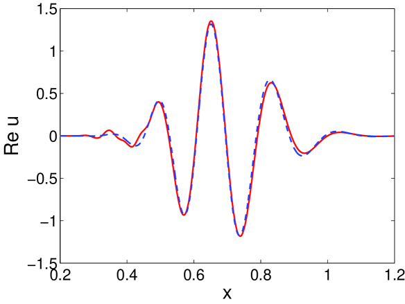
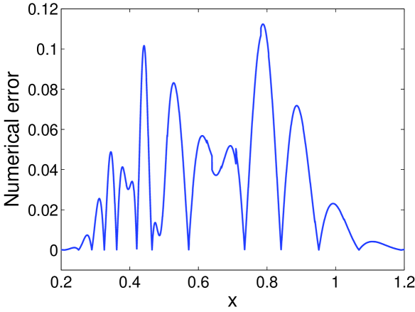
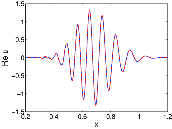
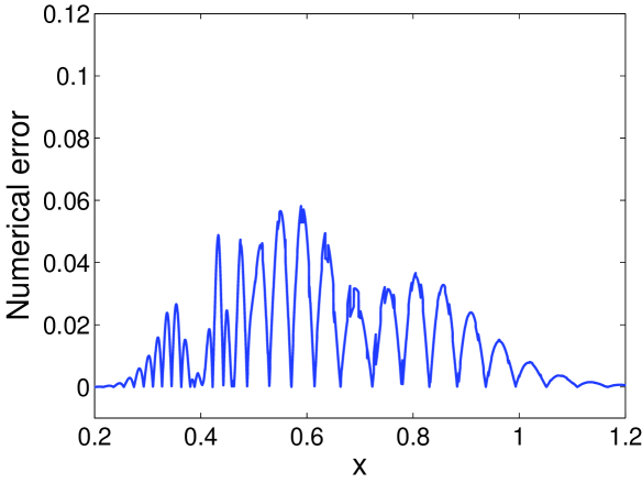
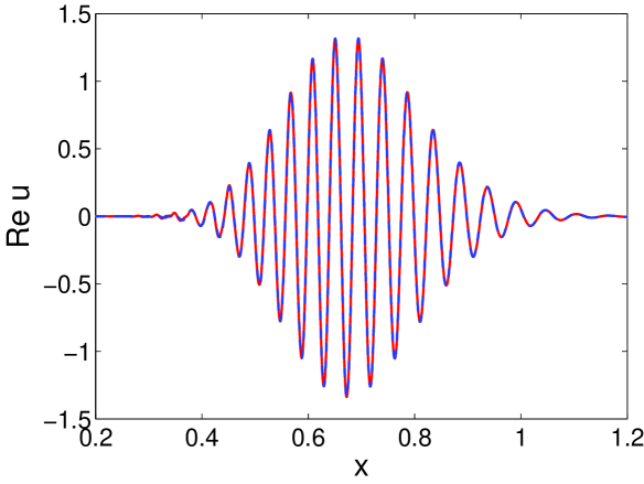
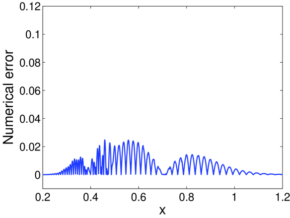
The final time is T=0.5𝑇0.5T=0.5. We plot the real part of the wave field obtained by FGA compared with the true solution in Figure 2 for ε=1/64, 1/128, 1/256𝜀16411281256\varepsilon=1/64,\;1/128,\;1/256. The true solution is computed by the finite difference method using the mesh size of δx=1/212𝛿𝑥1superscript212\delta x=1/2^{12} and the time step of δt=1/218𝛿𝑡1superscript218\delta t=1/2^{18} for domain [0,2]02[0,2]. Table 1 shows the superscript\ell^{\infty} and 2superscript2\ell^{2} errors of both the FGA solution uFGAsuperscript𝑢FGAu^{\mathrm{FGA}} and the GBM solution uGBMsuperscript𝑢GBMu^{\mathrm{GBM}}. The convergence orders in ε𝜀\varepsilon of superscript\ell^{\infty} and 2superscript2\ell^{2} norms are 1.081.081.08 and 1.171.171.17 separately for FGA, and 0.540.540.54 and 0.570.570.57 for GBM. We observe a better accuracy order of FGA than GBM.

We choose δt=1/211𝛿𝑡1superscript211\delta t=1/2^{11} for solving the ODEs and δx=1/212𝛿𝑥1superscript212\delta x=1/2^{12} to construct the final solution in both FGA and GBM. In FGA, we take δq=δp=δy=1/27,Nq=128,Np=45formulae-sequence𝛿𝑞𝛿𝑝𝛿𝑦1superscript27formulae-sequencesubscript𝑁𝑞128subscript𝑁𝑝45\delta q=\delta p=\delta y=1/2^{7},\;N_{q}=128,\;N_{p}=45 for ε=1/128, 1/256𝜀11281256\varepsilon=1/128,\;1/256 and δq=δp=δy=1/25,Nq=32,Np=33formulae-sequence𝛿𝑞𝛿𝑝𝛿𝑦1superscript25formulae-sequencesubscript𝑁𝑞32subscript𝑁𝑝33\delta q=\delta p=\delta y=1/2^{5},\;N_{q}=32,\;N_{p}=33 for ε=1/64𝜀164\varepsilon=1/64. In GBM, we take δy0=1/27,Ny0=128formulae-sequence𝛿subscript𝑦01superscript27subscript𝑁subscript𝑦0128\delta y_{0}=1/2^{7},\;N_{y_{0}}=128 for ε=1/128, 1/256𝜀11281256\varepsilon=1/128,\;1/256 and δy0=1/25,Ny0=32formulae-sequence𝛿subscript𝑦01superscript25subscript𝑁subscript𝑦032\delta y_{0}=1/2^{5},\;N_{y_{0}}=32 for ε=1/64𝜀164\varepsilon=1/64.

We remark that in this example the mesh sizes of p𝑝p and q𝑞q have been taken very small and Npsubscript𝑁𝑝N_{p} large enough to make sure that the error of FGA mostly comes from asymptotic expansion, but not from initial value decomposition, numerical integration of ODEs and so on. Such a choice of fine mesh is not necessary for the accuracy of FGA, as one can see in Example 4.3.

Table 1. Example 4.1, the superscript\ell^{\infty} and 2superscript2\ell^{2} errors for FGA and GBM.
ε𝜀\varepsilon 1/261superscript26{1}/{2^{6}} 1/271superscript27{1}/{2^{7}} 1/281superscript28{1}/{2^{8}}
uuFGAsubscriptdelimited-∥∥𝑢superscript𝑢FGAsuperscript\lVert u-u^{\mathrm{FGA}}\rVert_{\ell^{\infty}} 1.12×1011.12superscript1011.12\times 10^{-1} 6.18×1026.18superscript1026.18\times 10^{-2} 2.51×1022.51superscript1022.51\times 10^{-2}
uuFGA2subscriptdelimited-∥∥𝑢superscript𝑢FGAsuperscript2\lVert u-u^{\mathrm{FGA}}\rVert_{\ell^{2}} 6.05×1026.05superscript1026.05\times 10^{-2} 2.96×1022.96superscript1022.96\times 10^{-2} 1.19×1021.19superscript1021.19\times 10^{-2}
uuGBMsubscriptdelimited-∥∥𝑢superscript𝑢GBMsuperscript\lVert u-u^{\mathrm{GBM}}\rVert_{\ell^{\infty}} 7.15×1017.15superscript1017.15\times 10^{-1} 5.08×1015.08superscript1015.08\times 10^{-1} 3.36×1013.36superscript1013.36\times 10^{-1}
uuGBM2subscriptdelimited-∥∥𝑢superscript𝑢GBMsuperscript2\lVert u-u^{\mathrm{GBM}}\rVert_{\ell^{2}} 3.26×1013.26superscript1013.26\times 10^{-1} 2.28×1012.28superscript1012.28\times 10^{-1} 1.47×1011.47superscript1011.47\times 10^{-1}
Refer to caption
Refer to caption
(a) ε=164𝜀164\varepsilon=\frac{1}{64}
Refer to caption
Refer to caption
(b) ε=1128𝜀1128\varepsilon=\frac{1}{128}
Refer to caption
Refer to caption
(c) ε=1256𝜀1256\varepsilon=\frac{1}{256}
Figure 2. Example 4.1, the comparison of the true solution (solid line) and the solution by FGA (dashed line). Left: the real part of wave field; right: the errors between them.
Example 4.2.

The wave speed is c(x)=x2𝑐𝑥superscript𝑥2c(x)=x^{2}. The initial conditions are

u0=exp((x0.55)22ε)exp(ıxε),subscript𝑢0superscript𝑥0.5522𝜀italic-ı𝑥𝜀\displaystyle u_{0}=\exp\left(-\frac{(x-0.55)^{2}}{2\varepsilon}\right)\exp\left(\frac{\imath x}{\varepsilon}\right),
tu0=ıx2εexp((x0.55)22ε)exp(ıxε).subscript𝑡subscript𝑢0italic-ısuperscript𝑥2𝜀superscript𝑥0.5522𝜀italic-ı𝑥𝜀\displaystyle\partial_{t}u_{0}=-\frac{\imath x^{2}}{\varepsilon}\exp\left(-\frac{(x-0.55)^{2}}{2\varepsilon}\right)\exp\left(\frac{\imath x}{\varepsilon}\right).

We use this example to illustrate the performances of FGA and GBM when the beams spread in GBM. The final time is T=1.0𝑇1.0T=1.0 and ε=1/256𝜀1256\varepsilon=1/256. Remark that the initial condition is chosen as a single beam on purpose so that one can apply GBM without introducing any initial errors. The true solution is provided by the finite difference method using δx=1/211𝛿𝑥1superscript211\delta x=1/2^{11} and δt=1/217𝛿𝑡1superscript217\delta t=1/2^{17} for domain [0,4]04[0,4]. We take δq=δp=δy=1/27,Nq=128,Np=45formulae-sequence𝛿𝑞𝛿𝑝𝛿𝑦1superscript27formulae-sequencesubscript𝑁𝑞128subscript𝑁𝑝45\delta q=\delta p=\delta y=1/2^{7},\;N_{q}=128,\;N_{p}=45 in FGA to make sure that the error in the initial value decomposition of FGA is very small. The time step is δt=1/210𝛿𝑡1superscript210\delta t=1/2^{10} for solving the ODEs and the mesh size is chosen as δx=1/211𝛿𝑥1superscript211\delta x=1/2^{11} to construct the final solution in both FGA and GBM.

Figure 3 compares the amplitudes of the wave field computed by FGA and GBM, and the true solution. One can see that the beam has spread severely in GBM. The results confirm that FGA has a good performance even when the beam spreads, while GBM does not. Moreover, it does not help improving the accuracy if one uses more Gaussian beams to approximate the initial condition in GBM as shown in Figure 4, where Ny0=128subscript𝑁subscript𝑦0128N_{y_{0}}=128 beams are used initially and δy0=1/27𝛿subscript𝑦01superscript27\delta y_{0}=1/2^{7}. Remark that GBM can still give good approximation around beam center where Taylor expansion does not introduce large errors. This can be seen around x=1.2𝑥1.2x=1.2 in Figure 3.

Refer to caption
Refer to caption
Figure 3. Example 4.2, the comparison of the true solution (solid line), the solution by FGA (dashed line) and the solution by GBM (dots) for ε=1256𝜀1256\varepsilon=\frac{1}{256}. Left: the amplitude of wave field; right: the error between them (dashed line for FGA, dots for GBM).
Refer to caption
Refer to caption
Figure 4. Example 4.2, the comparison of the true solution (solid line) and the solution by GBM using multiple Gaussian initial representation (dots) for ε=1256𝜀1256\varepsilon=\frac{1}{256}. Left: the amplitude of wave field; right: the error between them.

4.2. Two dimension

Example 4.3.

The wave speed is c(x1,x2)=1𝑐subscript𝑥1subscript𝑥21c(x_{1},x_{2})=1. The initial conditions are

u0=exp(100(x12+x22))exp(ıε(x1+cos(2x2))),subscript𝑢0100superscriptsubscript𝑥12superscriptsubscript𝑥22italic-ı𝜀subscript𝑥12subscript𝑥2\displaystyle u_{0}=\exp\bigl{(}-100(x_{1}^{2}+x_{2}^{2})\bigr{)}\exp\left(\frac{\imath}{\varepsilon}(-x_{1}+\cos(2x_{2}))\right),
tu0=ıε1+4sin2(2x2)exp(100(x12+x22))exp(ıε(x1+cos(2x2))).subscript𝑡subscript𝑢0italic-ı𝜀14superscript22subscript𝑥2100superscriptsubscript𝑥12superscriptsubscript𝑥22italic-ı𝜀subscript𝑥12subscript𝑥2\displaystyle\partial_{t}u_{0}=-\frac{\imath}{\varepsilon}\sqrt{1+4\sin^{2}(2x_{2})}\exp\bigl{(}-100(x_{1}^{2}+x_{2}^{2})\bigr{)}\exp\left(\frac{\imath}{\varepsilon}(-x_{1}+\cos(2x_{2}))\right).

This example presents the cusp caustics shown in Figure 5. The final time is T=1.0𝑇1.0T=1.0. The true solution is given by the spectral method using the mesh δx1=δx2=1/512𝛿subscript𝑥1𝛿subscript𝑥21512\delta x_{1}=\delta x_{2}=1/512 for domain [1.5,0.5]×[1,1]1.50.511[-1.5,0.5]\times[-1,1]. We take δq1=δq2=δp1=δp2=δy1=δy2=1/32𝛿subscript𝑞1𝛿subscript𝑞2𝛿subscript𝑝1𝛿subscript𝑝2𝛿subscript𝑦1𝛿subscript𝑦2132\delta q_{1}=\delta q_{2}=\delta p_{1}=\delta p_{2}=\delta y_{1}=\delta y_{2}=1/32, Nq=32,Np=8formulae-sequencesubscript𝑁𝑞32subscript𝑁𝑝8N_{q}=32,\;N_{p}=8 in FGA, and use δx1=δx2=1/128𝛿subscript𝑥1𝛿subscript𝑥21128\delta x_{1}=\delta x_{2}=1/128 to reconstruct the solution. Figure 6 compares the wave amplitude of the true solution and the one by FGA for ε=1/128𝜀1128\varepsilon=1/128 and 1/25612561/256. The superscript\ell^{\infty} and 2superscript2\ell^{2} errors of the wave amplitude are 1.98×1011.98superscript1011.98\times 10^{-1} and 4.42×1024.42superscript1024.42\times 10^{-2} for ε=1/128𝜀1128\varepsilon=1/128, and 1.07×1011.07superscript1011.07\times 10^{-1} and 2.20×1022.20superscript1022.20\times 10^{-2} for ε=1/256𝜀1256\varepsilon=1/256. This shows a linear convergence in ε𝜀\varepsilon of the method.

Refer to caption
Refer to caption
Figure 5. Example 4.3, a set of the characteristic lines develops the cusp caustic.
Refer to caption
Refer to caption
(a) Frozen Gaussian approximation
Refer to caption
Refer to caption
(b) True solution
Refer to caption
Refer to caption
(c) Errors
Figure 6. Example 4.3, the comparison of the true solution and the solution by FGA. Left: wave amplitude of ε=1128𝜀1128\varepsilon=\frac{1}{128}; right: wave amplitude of ε=1256𝜀1256\varepsilon=\frac{1}{256}.

5. Discussion and Conclusion

We first briefly compare the efficiency of frozen Gaussian approximation (FGA) with the Gaussian beam method (GBM). GBM uses only one Gaussian function for each grid point in physical space, while FGA requires more Gaussians per grid point with different initial momentum to capture the behavior of focusing or spreading of the solution. However, the stationary phase approximation suggests that the number of Gaussians is only increased by a small constant multiple of the number of those used in GBM. In addition, in GBM one has to solve the Riccati equation, which is a coupled nonlinear ODE system in high dimension, to get the dynamics of the Hessian matrix for each Gaussian, while in FGA the Hessian matrix is determined initially and has no dynamics. Therefore, the overall efficiency of FGA is comparable to GBM.

Admittedly, higher order GBM gives better asymptotic accuracy, and only requires solving a constant number of additional ODEs as in FGA. The numerical cost of higher order GBM is comparable to FGA. However, higher order GBM has its drawbacks: The imaginary part of higher order (larger than two) tensor function dose not preserve positive definiteness in time evolution, which may destroy the decay property of the ansatz of higher order GBM . This is even more severe when beams spread. Moreover, the ODEs in higher order GBM are in the form of coupled nonlinear system in high dimension. It raises numerical difficulty caused by stability issues. We also note that, the numerical integration of ODEs in FGA can be easily parallelized since the Hamiltonian flow (2.4) is independent for different initial (𝒒,𝒑)𝒒𝒑(\boldsymbol{q},\boldsymbol{p}), while it is not so trivial for higher order tensors in GBM.

From the accuracy point of view, our numerical examples show that first order FGA method has asymptotic accuracy 𝒪(ε)𝒪𝜀\mathcal{O}(\varepsilon). The existing rigorous analysis ([CoRo:97, BoAkAl:09, LiRuTa:10]) proves that the k𝑘k-th order GBM has an accuracy of 𝒪(εk/2)𝒪superscript𝜀𝑘2\mathcal{O}(\varepsilon^{k/2}). Hence, at the first order, FGA has better asymptotic accuracy than GBM. We note that, however, there has been numerical evidence presenting 𝒪(ε)𝒪𝜀\mathcal{O}(\varepsilon) asymptotic accuracy order for first order GBM, for example in [JiWuYa:08, JiWuYa:11, MoRu:app, LiRuTa:10]. This phenomenon is usually attributed to error cancellation between different beams. To the best of our knowledge, the mechanism of error cancellation in GBM has not been systematically understood yet.

With the the gain of halfth order in asymptotic accuracy due to cancellation, the first order GBM has the same accuracy order as FGA (of course GBM still loses accuracy when beams spread). Remark that the gain in asymptotic accuracy order depends on the choice of norm. For example, the first order GBM has a halfth order convergence in superscript\ell^{\infty} norm, first order convergence in 2superscript2\ell^{2} norm and 3/2323/2-th order convergence in 1superscript1\ell^{1} norm in Example 111 of [JiWuYa:08]. Moreover, the error cancellation seems not to be easily observed in numerics unless ε𝜀\varepsilon is very small. For instance, the convergence order of GBM in Example 4.1 is only a bit better than 1/2121/2 for ε𝜀\varepsilon up to 1/25612561/256. While in FGA, we numerically observe the first order asymptotic accuracy in both 2superscript2\ell^{2} and superscript\ell^{\infty} norms.

Actually the accuracy of FGA can also be understood from a viewpoint of error cancellation. Note that the equalities (3.9), (3.10) and (3.11) in Lemma 3.2 play the role of determining the accuracy of FGA. In (3.9), the term 𝒙𝑸𝒙𝑸\boldsymbol{x}-\boldsymbol{Q} is of order 𝒪(ε)𝒪𝜀\mathcal{O}(\sqrt{\varepsilon}) due to the Gaussian factor, but after integration with respect to 𝒒𝒒\boldsymbol{q} and 𝒑𝒑\boldsymbol{p}, which is similar to the beam summation in GBM, it becomes 𝒪(ε)𝒪𝜀\mathcal{O}(\varepsilon). Similar improvement of order also happens in (3.10) and (3.11). Integration by parts along with (3.14) explains the mechanism of this type of error cancellation.

We conclude the paper as follows. In this work, we propose the frozen Gaussian approximation (FGA) for computation of high frequency wave propagation, motivated by the Herman-Kluk propagator in chemistry literature. This method is based on asymptotic analysis and constructs the solution using Gaussian functions with fixed widths that live on the phase plane. It not only provides an accurate asymptotic solution in the presence of caustics, but also resolves the problem in the Gaussian beam method (GBM) when beams spread. These merits are justified by numerical examples. Additionally, numerical examples also show that FGA exhibits better asymptotic accuracy than GBM. These advantages make FGA quite competitive for computing high frequency wave propagation.

For the purpose of presenting the idea simply and clearly, we only describe the method for the linear scalar wave equation using leading order approximation. The method can be generalized for solving other hyperbolic equations and systems with a character of high frequency. The higher order approximation can also be derived. Since the method is of Lagrangian type, the issue of divergence still remains, which will be resolved in an Eulerian framework. We present these results in the subsequent paper [LuYang:MMS].
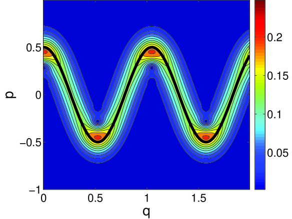
References