Effect of fractal disorder on static friction in the Tomlinson model

Abstract

We propose a modified version of the Tomlinson model for static friction between two chains of beads. We introduce disorder in terms of vacancies in the chain, and distribute the remaining beads in a scale invariant way. For this we utilize a generalized random Cantor set. We relate the static friction force, to the overlap distribution of the chains, and discuss how the distribution of the static friction force depends on the distribution of the remaining beads. For the random Cantor set we find a scaled distribution which is independent on the generation of the set.

I Introduction

Friction is a long studied phenomenon in physics bowden ; bnj ; braun . Still, the regime of validity and the microscopic origin of the empirical laws of static and dynamic friction (that goes under the name of Amontons-Coulomb) are not well established. But the advancements of technology in the last few decades has triggered both theoretical gnecco ; sang ; kajita ; capozza ; kawaguchi ; caroli2 , as well as experimental investigations in this field mate ; hirano .

Surfaces which appear smooth may contain roughness at the micrometer scale caroli as well as impurities in the contact region muser which will influence the friction properties of the materials. If we limit ourselves to the study of atomically clean surfaces, it is sufficient to consider the relative motion of the atomic layers in contact. The earliest attempt to model such a situation was carried out by Tomlinson tomlinson . Tomlinson’s model is a chain of beads, representing atoms, all of which are individually attached to a body above. The chain is dragged on a periodic potential representing a corrugated substrate (see Fig. 1 (a)). Each bead interacts with the potential, but there is no interaction among the beads. As in the Tomlinson model for dry friction (see e.g. weiss ), the surface atoms are considered to be independent oscillators capable of absorbing a finite energy and momentum. Although they are connected by the chain, the energy is assumed to get dissipated within the bulk and not transferred to the neighbouring atoms along the chain. This model has regained its importance in recent years because, in experiments using atomic force microscopy, the contact probe can be studied at an atomic level (see e.g., braun ). There are also a number of similar models using chains of beads moving over a substrate. Most notably is the Frenkel-Kontorova model fk1 , where the beads also interact with the nearest neighbors.

In this paper, we propose a modified version of the Tomlinson model. We consider a two chain version of the model, where one of the chains slides on top of the other (see Fig. 1 (b)). We study the effect of disorder in the static friction force. In particular, we introduce vacancy disorder, by removing beads, in both chains. We relate the static friction force to the measure of overlap of beads. The disorder in the chains is such that the remaining beads are distributed in a scale invariant way. For this we use a generalized version of the Cantor set. This leads to a certain kind of overlap distribution, and we compare this to other ways of distributing the beads, and discuss how this relates to the distribution of static friction force.

It may be mentioned at this point that rough surfaces have a self-affine character and therefore can be represented by self-similar fractals mandelbrot . We represent the disorder in the Tomlinson model by a generalized random Cantor set, which is one of the simplest examples of a fractal. Although the Cantor set is a purely mathematical construction, it has been studied extensively by physicist as it encapsulates the essential property of self-similarity and scale invariance.

The paper is organized in the following way: In section (II) we define the model. Then in section (III) we briefly discuss the basic definitions and useful properties of the Cantor set, which will be required in the subsequent discussions. In section (IV) we find the expressions for the static friction force distribution for Tomlinson’s model with beads distributed as random cantor sets. We conclude by summarizing the results in section (V).

II The Model

The static friction force $F_{s}$, is defined to be the minimum force needed to initiate sliding between two objects in contact. If the applied force exceeds this threshold $F>F_{s}$, the objects will move relative to each other. The presence of this force is due to a local minimum in the energy landscape of spatial configurations of the two objects. Two disordered surfaces may however have several configurations which correspond to local minima, and the static friction may have different values in the different configurations.

We consider a two chain version of Tomlinson’s model, where one chain slides on top of the other (see Fig. 1 (b)). We introduce defects in terms of vacancies (removed beads). The vacancies are introduced randomly, and are statistically identical in both chains. The spacings between the sites in the chain (either occupied by a bead or removed), are constant and equal in both chains.

The underlying chain gives rise to a substrate potential for the chain above. We assume that the interaction potential between the beads in the opposite chains are short ranged and attractive, such that the substrate potential is on the form of a series of potential wells, corresponding to the remaining beads of the chain below (see Fig. 1 (c)).

The potential energy of a configuration of this modified Tomlinson model will be determined by the sum of beads locked in potential wells. The static friction force of one bead locked in a potential well is determined by the maximum value of the derivative of the potential. We will not specify the functional form of the potential well, but we assume that the static friction force of one bead in a potential has a given value. The static friction force of a chain will therefore be directly proportional to the number of beads locked in potential wells.

If there were no disorder, the overlap would be constant and the static friction force per bead would also be constant. If, however, there is disorder in terms of vacancies, the number of locked beads (referred to as the overlap) will not be constant but will have a set of possible values. These values, and hence the static friction force, will follow a distribution.

We assume that the expected number of overlapping beads is given and investigate how the distribution vary around the expectation value. We will see that this distribution will have certain features if the beads (and the potential wells from the substrate) are distributed with a spatial correlation between them. This distribution will differ significantly from the case when the remaining beads (and the potential wells from the substrate) are distributed uniformly.

We are especially interested in the properties of the distribution when the beads are distributed with a spatial correlation which decays as a power-law in the distance between the beads, as this correspond to a fractal disorder in the chain. A binary chain (with vacant or occupied sites) is, however, not uniquely determined by the spatial correlation structure. We choose to utilize generalized random Cantor sets for the distribution of the remaining beads (see Fig. 3), as the random Cantor set has the desired correlation structure on an average (this is a result of the self-similar property of the set). Moreover the structure of the random Cantor set is simple enough to allow theoretical results for the overlap distribution.

Figure 1: (a) The Tomlinson model: A chain of beads being dragged with an applied force $F$ in a periodic potential $V(x)$. (b) a two chain version of the Tomlinson model, with defects in terms of vacancies. (c) Same as (b) with the potential from the underlying chain illustrated.

III Cantor sets

The prototype example of a fractal is the Cantor set $C$. The Cantor set is constructed by first removing the middle third of the base interval [0, 1]. From each of the remaining intervals, [0, 1/3] and [2/3, 1], a middle third is again removed. The process of removing middle thirds of the remaining intervals is continued ad infinitum. The intervals which are left after the middle third of every remaining interval have been removed $n$ times, is referred to as the Cantor set $C_{n}$, at generation $n$. $C_{n}$ becomes a true fractal as $n$ goes to infinity $\displaystyle C=\lim_{n\rightarrow\infty}C_{n}$.

There are two self-similar transformations related to the Cantor set $C$. The transformations are $S^{(1)}(x)=x/3$ and $S^{(2)}(x)=(x+2)/3$. We can describe the process of removing the middle third of every interval by the action of these transformation,

$$C_{n}=S^{(1)}(C_{n-1})\bigcup S^{(2)}(C_{n-1}).$$

And we can define $C$ to be the subset of $[0,1]$ which is invariant under the union of these two transformations. Fig. 2 illustrates the construction procedure.

Figure 2: Construction of a triadic Cantor set.

In order to investigate properties which emerge from the fractal nature of a subset of an interval, we will extend the notion of a Cantor set. We will construct a generalized Cantor set by the action of $r$ self-similar transformations on the interval [0, 1]. Let $a=\{a_{1},a_{2},...,a_{r}\}$ be a set of integers such that $1<r<s$ and $a_{i}<a_{j}$ for $i<j$. The self-similar transformations be on the following form:

$$S^{(i)}(x)=\frac{x+a_{i}-1}{s}.$$

And we will obtain the generalized Cantor set in the obvious way

$$C_{n}=\bigcup_{i}S^{(i)}(C_{n-1}).$$

The Cantor set constructed this way will consist of $r^{n}$ line elements of equal length that may or may not be connected. We identify the integers in $a$ as the positions of the remaining line elements at the first generation. The Box Counting dimension of this generalized Cantor set is given by $D_{B}=\log(r)/\log(s)$ (see e.g. falconer ), and the regular triadic Cantor set is obtained by taking $s=3$ and $a=\{1,3\}$.

The notion of a random Cantor set is ambiguous as we can randomize in several ways. We will define the random version of this generalized Cantor set analogous to Falconer’s definition of the triadic Cantor set in falconer . For each generational step, divide every remaining line element from the previous generation into $s$ elements of equal length and remove all but $r$ of them. For each line segment, and for each generation, randomize the position of the $r$ remaining intervals, but keep the number of remaining intervals fixed. The self-similar properties of this set hold only in a statistical sense.

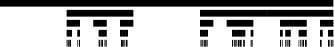
Figure 3: Construction of a random Cantor set, $s=5$ and $r=3$.

The generalized Cantor set will at generation $n$ consist of $r^{n}$ of the $s^{n}$ equal distant parts of the interval [0,1]. This enables us to represent it as a vector $(C_{n,1},C_{n,2},...,C_{n,s^{n}})$. The vector element $C_{n,i}$ represent the $i$th interval of the Cantor set such that $C_{n,i}$ takes the value 1 if the interval $[(i-1)/s,i/s]$ is contained in $C_{n}$, and the value 0 if it is removed. The vector contains therefore $s^{n}$ elements, out of which $r^{n}$ takes the value 1, and the rest takes the value 0.

The Cantor set is of measure zero. That is, the size of the Cantor set (sum of the remaining line segments), will go to zero as the generation goes to infinity. For that reason we study the Cantor set at a finite generation, at the atomic level there is, of course, no way to continue the removal procedure.

IV Overlap

IV.1 Overlap of random sets

Let us first consider the overlap of two chains with randomly placed vacancies, uniformly distributed along the chain. The overlap distribution is trivial, but we include it here as it will be instructive to compare it with the other results.

Consider two independently generated vectors $\left(X_{1},...,X_{N}\right)$, $\left(X^{\prime}_{1},...,X^{\prime}_{N}\right)$ containing $N$ binary variates representing the chain (0 represents a removed bead at a given site). Each element takes the value 1 with probability $p$. The probability of an overlap at element $i$ is therefore $\Pr(X_{i}=1,X^{\prime}_{i}=1)=p^{2}$. The overlap of the two vectors is given by $Y=\sum X_{i}X^{\prime}_{i}$. And the overlap distribution is on the form of a binomial distribution:

$$\Pr(Y=x)={N\choose x}p^{2x}(1-p^{2})^{N-x}.$$ (1)

IV.2 Overlap of random Cantor sets

In order to describe the overlap distribution for two random (independently generated) Cantor sets, $C_{n,i}$ and $C^{\prime}_{n,i}$, it is instructive to consider first the overlap of two random triadic Cantor sets ($s=3,r=2$), without a relative displacement as illustrated in Fig. 4 (a). Notice, however, that Fig. 4 also illustrates the construction of the Cantor sets. The figure does not suggest that the Cantor set is embedded in two dimensions. The overlap at generation $n$ is given by $Y_{n}=\sum C_{n,i}C^{\prime}_{n,i}$. For $n=1$ one can easily calculate, by summing up the possible outcomes, that the probability distribution of the overlap takes the following form

$$\Pr(Y_{1}=0) =0,$$

$$\Pr(Y_{1}=1) =2/3,$$

$$\Pr(Y_{1}=2) =1/3.$$

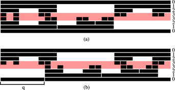
Figure 4: (Color online) The overlap of two (independently generated) random Cantor sets at generation 3 ($s=3,r=2$). The generation number of the two sets are marked on the right side. (a) shows the overlap when the sets are perfectly aligned, and (b) shows the overlap when the sets are shifted relatively by an offset $q$. The overlap size is the number of overlapping elements at the final generation of the opposite sets (in the shaded region). The number of overlapping elements are 3 for both (a) and (b).

Call $A$ the event that only one element overlap at the first generation of the construction, and $B$ the event that two elements overlap at the first generation of the construction. $A$ and $B$ are mutually exclusive events, and $P(A)+P(B)=1$. Consider the case when $(C_{n,i})$ is constructed by an iterative procedure like in Fig. 3. We can write the following relation

$$\Pr(Y_{n}=x)=\frac{2}{3}\Pr(Y_{n}=x|A)+\frac{1}{3}\Pr(Y_{n}=x|B).$$

Note that

$$\Pr(Y_{n}=x|A) =\Pr(Y_{n-1}=x),$$

$$\Pr(Y_{n}=x|B) =\sum_{i\leq x}\Pr(Y_{n-1}=x-i)\Pr(Y_{n-1}=i).$$

So we have

$$\quad\Pr(Y_{n}=x)=$$

$$\frac{2}{3}\Pr(Y_{n-1}=x)+\frac{1}{3}\sum_{i\leq x}\Pr(Y_{n-1}=x-i)\Pr(Y_{n-1}=i).$$

As $n$ grows large, we can approximate this by a continuous distribution $f_{n}(x)=\Pr(Y_{n}=x)$. The equation above translate to the following equation:

$$f_{n}(x)=\frac{2}{3}f_{n-1}(x)+\frac{1}{3}(f_{n-1}\ast f_{n-1})(x),$$ (2)

where $(a\ast b)(x)$ is the convolution $\int_{-\infty}^{\infty}a(y)b(x-y)\,\mathrm{d}y$, and $f_{n}(x)=0$ for $x<0$. The overlap difference between two consecutive generations in the limit of large $n$, should not alter the qualitative behavior of the probability distribution. We therefore assume that there is a $n$-independent distribution $f$ such that

$$f_{n}(x)=f(x/\mu^{n})/\mu^{n},$$ (3)

for a scaling variable $\mu$. This is verified by numerical calculations, with $\mu=\langle Y_{1}\rangle=r^{2}/s=4/3$ which is the expected overlap at the first generation. $f(x)$ should then obey the equation

$$f(x/\mu)/\mu=\frac{2}{3}f(x)+\frac{1}{3}(f\ast f)(x).$$ (4)

To proceed with this functional equation we can take the Fourier transform on both sides. Using the elementary properties of the Fourier transformation we get

$$\tilde{f}(k\mu)=\frac{2}{3}\tilde{f}(k)+\frac{1}{3}\tilde{f}(k)^{2}.$$

If we assume that $\tilde{f}(k)$ is analytical in the complex plane, we can expand it as $\tilde{f}(k)=\sum a_{j}k^{j}$. By matching terms we get a family of solutions

$$a_{0}=1,\,\,\,a_{1}\in\mathbb{C},\,\,\,a_{n}=\frac{1}{4\left(\mu^{n-1}-1\right)}\sum_{j=1}^{n-1}a_{j}a_{n-j},\,n>2.$$

The real part of $\tilde{f}(k)$ has to be even, and the imaginary part has to be odd to make $f(x)$ real. We therefore choose $a_{1}$ to be purely imaginary.

Note that the Fourier transform is identical to the characteristic function $\varphi(k)=\langle\exp(ikx)\rangle$ of $f(x)$. The moments of the distribution is given by the relation $\langle x^{m}\rangle=(-i)^{m}\varphi^{(m)}(0)$. The first moment of $f(x)$ is by construction one, $\langle x\rangle=1$, so we choose $a_{1}=i$. ($a_{0}=1$ is consistent with the normalization of $f(x)$.) All other moments are specified by

$$\langle x^{m}\rangle=(-i)^{m}\,m!\,a_{m},$$ (5)

and the probability distribution $f(x)$, is uniquely determined in terms of its moments.

For the general random Cantor set, defined in the previous section, we have the following results. For the overlap probability for the first generation we have

$$\Pr(Y_{1}^{(s,r)}=x)=p^{(s,r)}(x)=\frac{{r\choose x}{s-r\choose r-x}}{{s\choose r}}.$$

Analogous to the distribution in eqn. (2), we have that the overlap distribution for the general case should be of the form

$$f_{n}^{(s,r)}(x)=\sum_{j=1}^{r}p^{(s,r)}(j)\left(\underbrace{f_{n-1}^{(s,r)}\ast\dots\ast f_{n-1}^{(s,r)}}_{j-1\text{ times}}\right)(x),$$ (6)

and the $n$ invariant distribution $f^{(s,r)}(x)$ is given by

$$f^{(s,r)}(x/\mu)/\mu=\sum_{j=1}^{r}p^{(s,r)}(j)\left(\underbrace{f^{(s,r)}\ast\dots\ast f^{(s,r)}}_{j-1\text{ times}}\right)(x),$$ (7)

with $\mu=r^{2}/s$. By expanding the Fourier transform of $f^{(s,r)}(x)$ as an analytical function, we can specify the moments for the probability distribution as we did in eqn. (5), but the values of $s$ and $r$ have to be specified to do so.

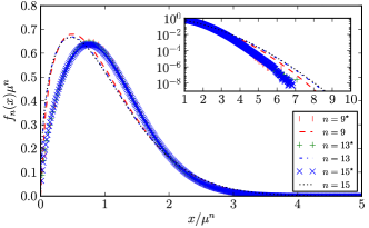
(a)

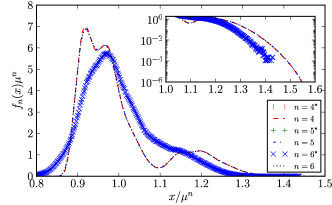
(b)

Figure 5: (Color online) The collapse of the overlap distribution for different generations ($n$ values). (a) for $s,r=3,2$ and (b) for $s,r=6,5$. The overlap distribution marked with lines are for random cantor sets, and are generated by eqn. (6). The overlap distribution marked with points (marked by an asterisk * in the legend), are for random cantor sets with a randomized offset, and are generated by sampling. The $x$ axis is in units of expected overlap. The embedded plot shows the same in log scale for the $y$-axis.

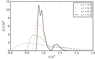
(a)

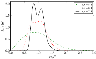
(b)

Figure 6: (Color online) The $n$ invariant overlap distribution, generated by eqn. (6), for different values of $s,r$, with (a) $s-r=1$, and (b) $s-r=2$. the $x$ axis is in units of expected overlap.

Up until now we have considered the overlap of the random Cantor sets without any offset, i.e. the Cantor sets are placed such that the first element of the top Cantor set (vector element $C_{n,1}$) overlap the first element of the lower Cantor set (see Fig. 4 (a)). In order to study the overlap when we also have a random offset, we assume periodic boundary conditions as indicated by Fig. 4 (b). There is no obvious way to construct an analytical expression for the distribution with the randomized offset, but we can generate the distributions numerically. Fig. 5 shows how the overlap distribution converges to the $n$-invariant distribution with and without a randomized offset, for (a) $s,r=3,2$, and (b) $s,r=6,5$.

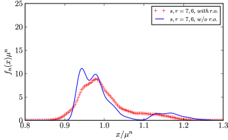
(a)

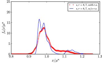
(b)

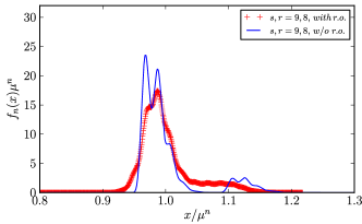
(c)

Figure 7: (Color online) The overlap distribution for $s-r=1$ when $r/s$ goes to 1. $s,r=7,6$ in (a), $8,7$ in (b) and $9,8$ in (c). Lines (w/o randomized offset) are generated by eqn. (6). Points (with randomized offset) are generated by sampling. The $x$ axis is in units of expected overlap.

Fig. 6 (a) shows the distributions for different values of $s$ with $r=s-1$, and Fig. 6 (b) shows the same for $r=s-2$. The distributions are generated by eqn. (6). Fig. 7 shows how the overlap distributions behave for $s-r=1$ when the ratio $r/s$ goes to one. The overlap distribution with a randomized offset is generated by sampling over the overlap for 1000 different configurations and for all the possible offsets.

V Summary and Discussion

We model the static friction force between two atomically smooth surfaces by a two-chain version of Tomlinson’s model. We consider substitutional defects in terms of vacancies along both chains (see Fig. 1). The static friction force is assumed to be directly proportional to the number of beads in the upper chain which are locked in the potential wells in the potential arising from the chain beneath. This number is modeled by the overlap of two binary chains with a given correlation structure. We are in particular interested in the strong disorder limit where self-similarity may appear. The self-similarity translates to the power-law correlation in the spatial displacements of the remaining beads. The main motivation to consider this is the fact that the height profile of rough surfaces often has a fractal (self-similar) property (see e.g. mandelbrot ).

A generalized random Cantor set is utilized to capture such properties. This Cantor set is generated by removing all but $r$ out of $s$ segments from each remaining element at each generation. This procedure is explained in detail in section III. The remaining beads in the chain are distributed according to this random Cantor set. We study both the cases of with and without a random relative offset between the Cantor sets (as illustrated in Fig. 4). The overlap of two chains is assumed to give the static friction force. Hence, the distribution of the static friction force is given by the distribution of the overlap of the Cantor sets.

It may be noted here that the earlier applications of two fractal overlap models chakrabarti ; bhattacharyya ; pathikrit1 , in the context of earthquake dynamics, focused on the time series of the overlap of regular (non-random) Cantor sets. Our interest here is the overlap of random Cantor sets in the context of static friction.

Cantor sets have already been used to represent the scale invariance property of the contact area overlap between two plastic surfaces of macroscopic objects in the study by Warren and Krajcinovic warren . Their model does not represent similar properties of each of the surfaces, as in our model. In the model presented here, Cantor sets (embedded in one dimension) are used to represent each of the surface and we calculate the overlap profile between them. Warren and Krajcinovic, on the other hand, use Cantor sets embedded in two dimensions, and calculate how it overlaps with a plane surface. As such, our model is different and the results are not comparable.

For the overlap of the generalized random Cantor sets, without the randomized offset, we have found a recurrence relation for the distribution (eqn. (6)). Moreover we find that this distribution follows a scaling structure (eqn. (3)). This scaling leads to a distribution which is independent of the generation $n$ (though dependent on values of $s$ and $r$). We further show how one can specify the distribution uniquely in terms of the moments, and do the calculation explicitly for the case when $s=3$ and $r=2$ (see eqn. (5)).

After introducing a randomized offset between the Cantor sets (with periodic boundary conditions), we no longer have a recurrence relation, but we find numerically similar qualitative behavior. The distribution for the case with a randomized offset shows the same $n$ independent scaling behavior as the distribution without a randomized offset. Moreover, the distribution is shifted to slightly higher values of overlap as shown in Fig. 5. The same behavior is seen for different values of $s$ and $r$. The embedded log plot in Fig. 5 shows that the tail behavior falls faster than exponential in both cases.

When we look at the distribution for different values of $s$ and $r$, generated by eqn. (6), we see the emergence of multiple local maxima. This is a property of the sum of convolutions coming from eqn. (6), and depends on the allowed values of overlap for the first generation. These local maxima are averaged out when we look at the case with a randomized offset (see Fig. 5 and Fig. 7). We have conveniently presented the overlap distributions in units of the expected overlap (the actual overlap of a given set is found by multiplying the $x$ axis with $\mu^{n}=(r^{2}/s)^{n}$).

For a realistic chain for beads with vacancies, we can not assume that the remaining beads are distributed according to precise values of $s$ and $r$. Nor can we assume that the overlap distribution is as for two Cantor sets without randomizing a relative offset. If we consider the limit where $r/s$ approaches unity, (i.e. the limit where only a small fraction of beads are removed at every generation), we find for the overlap distribution with a randomized offset, that the shape of the distributions have some common general properties. The distribution gets a peak at the expected overlap, but also an interval with a non-zero probability for values higher than the expected overlap, see Fig. 7.

The overlap of beads distributed as a Cantor set is qualitatively very different from the overlap of uniformly displaced beads. To compare the distribution with that in Fig. 6, set $p=(r/s)^{n}$ and $N=s^{n}$ in eqn. (1). The resulting distribution would then be approximated by a Gaussian in the limit of large $n$, with mean $Np^{2}=(r^{2}/s)^{n}$ and a variance $Np^{2}(1-p^{2})=(r^{2}/s)^{n}(1-(r^{2}/s)^{n})$. This would correspond to a single peak at $x/\mu^{n}=1$ in Figs. 5-7. On the contrary the static friction force distribution for chain models, where the remaining beads are distributed in a scale invariant way, will not converge to a delta peak distribution but rather would be like that for Cantor sets with a randomized offset as in Figs. 5-7.

It is hard to compare our results with experimental data on microscopic dry friction between surfaces having scale invariant disorder. Surfaces having microscopic self-affine disorder have been studied using AFM fractalafm , but we are unfortunately not aware of any study where the static friction force between two such surfaces have been considered. We would like to mention that the above results for the distribution microscopic friction qualitatively agrees with the observation of similar distributions of the friction coefficient of Aluminium alloys under cold rolling (see e.g., liu ). Such an analysis can also be effectively utilized for comparing the distributions for dry friction coefficients between plastic rock surfaces having well known scaling properties of asperities. However, in a different context of studying the effect of multiscale roughness on contact mechanics, similar analysis has already been done (see e.g., sokoloff ).

References

- (1) F. P. Bowden and D. Tabor, The friction and Lubrication of Solids (Clarendon Press, Oxford, 1954)
- (2) B. N. J. Persson, Sliding Friction: Physical Principles and Application (2nd ed., Springer, Berlin, 2000)
- (3) O. M. Baun and A. G. Naumovets, Surf. Sc. Rep. 60, 79 (2006)
- (4) E. Gnecco, R. Bennewitz, T. Gyalog, C. Loppacher, M. Bammerlin, E. Meyer, and H. J. Guntherodt, Phys. Rev. Lett. 84, 1172 (2000)
- (5) Y. Sang, M. Dube, and M. Grant, Phys. Rev. lett. 87, 174301 (2001)
- (6) S. Kajita, H. Washizu, and T. Ohomori, Europhys. Lett. 87, 66002 (2009)
- (7) R. Capozza, A. Vanossi, A. Vezzani, and S. Zapperi, Phys. Rev. Lett. 103, 085502 (2009)
- (8) T. Kawaguchi and H. Matsukawa, Phys. Rev. B 56, 4261 (1997)
- (9) F. Heslot, T. Baumberger, B. Perrin, B. Caroli, and C. Caroli, Phys. Rev. E 49, 4973 (1994)
- (10) C. M. Mate, G. McClelland, R. Erlandsson, and S. Chiang, Phys. Rev. Lett. 59, 1942 (1987)
- (11) M. Hirano, K. Shinjo, R. Kaneko, and Y. Murata, Phys. Rev. Lett. 78, 1448 (1997)
- (12) T. Baumberger, P. Berthoud, and C. Caroli, Phys. Rev. B 60, 3928 (1999)
- (13) G. He, M. Muser, and M. Robbins, Science 284, 5420 (1999)
- (14) G. A. Tomlinson, Philos. Mag. 7, 905 (1929)
- (15) M. Weiss and F. J. Elmer, Phys. Rev. B 53, 7539 (1996)
- (16) Y. Frenkel and T. Kontorova, Zh. Eksp. Teor. Phys. 8, 1340 (1938)
- (17) B. B. Mandelbrot, The Fractal Geometry of nature (Freeman, San Francisco, 1982)
- (18) K. Falconer, Fractal Geometry and its Applications (Wiley, Chichester, 1999)
- (19) B. K. Chakrabarti and R. B. Stinchcombe, Physica A 270, 27 (1999)
- (20) P. Bhattacharyya, Physica A 348, 199 (2005)
- (21) P. Bhattacharya, B. K. Chakrabarti, Kamal, and D. Samanta, in Reviews of Nonlinear Dynamics and Complexity, edited by H. G. Schuster (Wiley - VCH, Weinheim, 2009) pp. 107–158
- (22) T. L. Warren and D. Krajcinovic, Wear 196, 1 (1996)
- (23) R. Buzio, C. Boragno, and U. Valbusa, Wear 254, 917 (2003)
- (24) Y. J. Liu, D. D. Tieu, A. K. adn Wang, and D. Yuen, J. Mat. Process. Tech. 111, 142 (2001)
- (25) J. B. Sokoloff, Phys. Rev. E. 78, 036111 (2008)