University of Liège
Faculty of Sciences
AGO Department
IFPA Academic year 2007-2008 Exotic and Non-Exotic Baryon Properties
on the Light Cone

 

Acknowledgment

First I would like to warmly thank my supervisor M. Polyakov for accepting me as a Ph.D. student, for his faith in me and especially for his kindness. It was a genuine pleasure to work and discuss with him. Thanks to him I have learned a lot on physics and the scientific world and met many very interesting people. Next I would like to express my gratitude towards J. Cugnon for his help, advice and support in all the necessary steps linked to the present thesis. I am especially grateful to K. Goeke and M. Hacke for the two years passed in Ruhr Universität Bochum (Germany) where the biggest part of the present thesis has been achieved. I will forever remember the welcoming people of Theoretische Physik II group. I have particularly appreciated everyday K. Goeke’s good humour. He was always whistling, laughing or in raptures about other physicists’ research. Living in Germany was a unique and extraordinary experience for me. That is the reason why I address this sentence to all people met there: Ich danke euch für alles. I would also like to thank D. Diakonov for his help, patience and disponibility. Beside being a great physicist he is also a man full of humanity. The other part of the present thesis has been achieved in Liège University. I am thankful to members of the IFPA group. I am in fact also indebted to all my teachers and professors for the share of their knowledge and passion.
A thesis work does not only consist of passing all the days in front of a computer, papers or drafts. Discussions about physics, pataphysics and metaphysics are also essential to proceed. So I am thankful for all the entertaining, pleasant, interesting, serious and less serious moments passed with friends and other people met. I cannot of course cite all of them: Alice D., Aline D., Christophe B., Daniel H., Danielle R., Delphine D., Denis F., Frédéric K., Geoffrey M., Ghil-Soek Y., Grégory A., Jacqueline M., Jean-Paul M., Jérémie G., Kirill S., Lionel H., Luc L., Michel W., Nina G., Pauline M., Quentin J., Renaud V., Sophie P., Stéphane T., Thibaut M., Tim L., Virginie C., Virgine D., Xavier C. and many others.
Finally I would like to express my gratitude to my family: my mother, my sister and my father for their love, presence, help and for giving me the possibility to reach my dreams. I have also special thanks for Pierrot Di Marco and his two sons Christophe and Sébastien. Thanks for all what they did for us. I am really happy and proud to consider them as genuine part of our family.

Chapter 1 Introduction

1.1 Hadron structure and QCD

One of the main objectives in Physics is to understand the structure and properties of matter. The dream would be to find the ultimate constituents with which one can build the whole universe. These ultimate constituents have, by definition, no internal structure and are called fundamental particles. The properties of any matter should in principle be deduced and/or explained starting from the fundamental particles and their dynamics.

The question of hadron structure is a rather old one. Fermi-Yang [1] and Sakata models [2] might be considered as first studies of this question. Both models considered the proton as a fundamental particle. Later, thanks to Deep Inelastic Scattering (DIS) experiments [3] at SLAC, it was realized that the nucleon was not a fundamental particle. Indeed, the observation in DIS of scaling phenomenon predicted by Bjørken [5] was the first direct evidence for the existence of point-like constituents in the nucleon. These point-like constituents were found to be charged spin-1/2 particles and were called partons. A simple and intuitive picture for explaining the scaling behavior is the parton model proposed by Feynman [6] in which the electron-nucleon DIS is described as an incoherent sum of elastic electron-parton scattering. The nature of these partons was however not specified. The uncalculable nucleon structure functions can then be expressed in terms of Parton Distribution Functions (PDF).

On the spectroscopic side, in view of the huge number of observed hadrons, Gell-mann [7] and Zweig [8] proposed in 1964 the quark model of hadrons. In this model hadrons can be grouped together in multiplets of a flavor $SU(3)$ symmetry. The (non-trivial) fundamental representation has dimension 3 and its elements are called quarks. Baryons then appear as systems of three strongly bound quarks and mesons as systems of a quark strongly bound to an antiquark.

Partons observed in DIS were initially identified with quarks. They have however a qualitative different behavior. While quarks are strongly bound in hadrons, partons appeared in DIS as almost free particles. This difference did not hurt much at that time. On the contrary, the phenomenological success of $SU(6)$ Naive Quark Model (NQM) in explaining hadron properties and the evidence for the existence of partons inside hadrons motivated the development of a new theory of strong interaction in 1973, namely the Quantum ChromoDynamics (QCD) [9]. The weakly interacting partons revealed in DIS and the fact that no free quark has been discovered in all the experiments performed are explained in QCD thanks to the asymptotic freedom and confinement properties respectively. The weak interacting high energy processes can be calculated and tested thanks to the asymptotic freedom property and gave a strong support to establish QCD as the correct theory of strong interaction.

By solving QCD one could thus in principle understand the structure as well as low-energy interactions and properties of all hadrons in terms of quarks and gluons. Unfortunately they cannot be easily calculated since the confinement property of QCD forbids an obvious and standard perturbative approach. The proposed way out is to study QCD numerically on a lattice. Many results have been obtained but are not quite reliable because of many numerical uncertainties due to lattice size and spacing, unprecise extrapolations to physical masses, …One of the major problems is of course the required computation time.

1.2 Models and degrees of freedom

Due to the huge difficulty encountered in solving QCD in the non-perturbative regime many models have been developed to understand and predict as far as possible hadron properties. For example, perturbative QCD can predict only the $Q^{2}$ dependence of PDF whereas it can say nothing about the PDF at a prescribed energy scale. These PDF are thus expected to be given by a low-energy model of QCD. The present models are more or less inspired from QCD and differ by the effective degrees of freedom they emphasize [10, 11]. While QCD plays with quarks and gluons as fundamental degrees of freedom, they could be inappropriate for a low-energy description.

1.2.1 Constituent quark models

The Naive Quark Model (NQM) is among the most successful models in explaining hadron properties [12] and hadron interactions [13]. This is also the most popular and intuitive picture of hadron internal structure. The most striking feature of NQM is that it gives a very simple but quite successful explanation of the static baryon properties, e.g. baryon spectroscopy and magnetic moments, by means of effective constituent quarks and nothing else. These constituent quarks are needed in hadron spectroscopy but have mass much larger than current quarks revealed in DIS experiments. The relation between constituent and current quarks can be considered as the holy grail of hadron physics. In NQM constituent quarks are non-relativistic (they are all considered to be in the $s$ state) and the baryon spin-flavor structure is given by $SU(6)$ symmetry. Many variations of NQM exist and are collectively called Constituent Quark Models (CQM). All these models, based on the effective degrees of freedom of valence constituent quarks and on $SU(6)$ spin-flavor symmetry, also contain a long-range linear confining potential and a $SU(6)$-breaking term like One-Gluon-Exchange (OGE), Goldstone-Boson-Exchange (GBE) or even Instanton-Induced (II) interaction.

While they are able to give good results for the static properties of the hadrons (spectrum, magnetic moments), they all fail to reproduce the dynamic ones, like electromagnetic transition form factors at low $Q^{2}$. A systematic lack of strength is observed at low $Q^{2}$. This seems to be a problem of degrees of freedom. Indeed, the region of low $Q^{2}$ corresponds to high distance, in which the creation of quark-antiquark pair degrees of freedom has a higher probability.

1.2.2 Quark-antiquark pairs and the nucleon sea

DIS experiments have shown a large enhancement of the cross sections at small Bjørken $x$, the fraction of nucleon momentum carried by the partons. This is related to the fact that the structure function $F_{2}(x)$ approaches a constant value as $x\to 0$ [14]. If the proton consists of only three valence quarks or any finite number of quarks, $F_{2}(x)$ is expected to vanish as $x\to 0$. It was then realized that valence quarks alone are not sufficient. Bjørken and Pascho [15] therefore assumed that the nucleon consists of three quarks in a background of an infinite number of quark-antiquark pairs. Kuti and Weisskopf [16] further included gluons among the constituents of nucleons in order to account for the missing momentum not carried by the quarks and antiquarks.

Quark-antiquark pairs are very important in the nucleon. This is in sharp contrast with the atomic system where particle-antiparticle pairs play a relatively minor role. In strong interaction, quark-antiquark pairs are readily produced as a result of the relatively large magnitude of the strong coupling constant $\alpha_{S}$. In CQM they are however not considered as degrees of freedom. Constituent quarks can be viewed as non-perturbative objects, current quarks dressed by a cloud of quark-antiquark pairs and gluons. This picture is however not realistic since CQM, which are supposed to model QCD at low energy, completely forget a very important approximate symmetry of QCD, namely chiral symmetry.

1.2.3 Chiral symmetry of QCD

The six observed quark flavors can be separated into light ($u,d,s$) and heavy flavors ($c,b,t$). As the masses of heavy and light quarks are separated by the same scale ($\simeq 1$ GeV) as the perturbative and non-perturbative regime, one may expect different physics associated with those two kinds of quarks. It appeared that physics of light quarks is governed by chiral symmetry. Since we are interested in this thesis only in light baryons, we will completely forget about the heavy flavors. Light baryons being composed of light quarks, chiral symmetry is expected to be crucial in the study of (light) baryon properties.

If the masses of light quarks are put to zero, then QCD Lagrangian becomes invariant under $SU(3)_{R}\times SU(3)_{L}$, the chiral flavor group. This symmetry implies that left- and right-handed quarks independently undergo a chiral rotation under the action of the group. According to Noether’s theorem [17] every continuous symmetry of the Lagrangian is associated to a four-current whose four-divergence vanishes. This in turn implies a conserved charge as a constant of motion. There are consequently sixteen conserved charges: eight vector and eight (pseudoscalar) chiral charges $Q_{5}^{a}$. One has

$$\left[Q_{5}^{a},H_{\textrm{QCD}}\right]=0$$ (1.1)

meaning that the chiral charges are conserved and that QCD Hamiltonian $H_{\textrm{QCD}}$ is chirally invariant. Under parity transformation axial charges change sign $Q_{5}^{a}\to-Q_{5}^{a}$. One expects thus (nearly) degenerate parity doublets in nature which do not exist empirically. The splitting in mass between particles of opposite parities is too large to be explained by the small current quark masses which break explicitly chiral symmetry ($m_{u}\simeq 4$ MeV, $m_{d}\simeq 7$ MeV and $m_{s}\simeq 150$ MeV).

The only explanation is that chiral symmetry is spontaneously broken. This means that the QCD Hamiltonian is invariant under chiral transformations whereas QCD ground state (i.e. the vacuum $|\Omega\rangle$) is not chirally invariant $Q_{5}^{a}|\Omega\rangle\neq 0$. For this reason, there must exist a non-vanishing vacuum expectation value (VEV), the chiral or quark condensate

$$\langle\bar{\psi}\psi\rangle=\langle\bar{\psi}_{R}\psi_{L}+\bar{\psi}_{L}\psi_{R}\rangle\simeq-(250\textrm{ MeV})^{3}$$ (1.2)

at the scale of a few hundred MeV. This condensate is not chirally invariant since it mixes left (L) and right (R) components and therefore serves as an order parameter of the symmetry breaking.

Goldstone theorem [18] states that to any spontaneously broken symmetry generator is associated a massless boson with the quantum numbers of this generator. Since we have eight spontaneously broken chiral generators, we can expect that in massless QCD there should exist an octet of massless pseudoscalar mesons. In real QCD current quarks have masses and the pseudoscalar mesons are expected to be also massive but relatively light. These Goldstone bosons are identified to the lightest meson octet ($\pi^{0},\pi^{\pm},K^{0},\bar{K}^{0},K^{\pm},\eta$).

Spontaneous Chiral Symmetry Breaking (SCSB) implies thus that QCD vacuum is non-trivial: it must contain quark-antiquark pairs with spins and momenta aligned in a way consistent with vacuum quantum numbers. It also implies that a massless quark develops a non-zero dynamical mass in this non-trivial vacuum. This mass depends in general on the momentum $p$. At small momentum it can be estimated to one half of the $\rho$ meson mass or one third of the nucleon mass $M(0)\approx 350$ MeV. Constituent quarks can then be seen as current quarks dressed by the mechanism of SCSB explaining the origin of 93% of light baryon masses. Let us also emphasize another important consequence of SCSB, the fact that quarks get a strong coupling with pions $g_{\pi qq}(0)=M(0)/F_{\pi}\simeq 4$ which is roughly one third of the pion-nucleon coupling constant $g_{\pi NN}\simeq 13.3$.

Let us stress that chiral symmetry has nothing to say about the mechanism of confinement which is presumably a totally different story. This is reflected in the instanton model of QCD vacuum [19] which explains many facts of low-energy hadronic physics but is known not to yield confinement. It is therefore possible that confinement is not particularly relevant for the understanding of hadron structure.

Application of QCD sum rules [20] to nucleons pioneered by B.L. Ioffe [21] provided several important lessons. One is that the physics of nucleons is heavily dominated by effects of the SCSB. This can be seen by the fact that all Ioffe’s formulae for nucleon observables, including nucleon mass itself, are expressed through the SCSB order parameter $\langle\bar{\psi}\psi\rangle$. It is therefore hopeless to build a realistic theory of the nucleon without taking into due account the SCSB.

1.2.4 Importance of pions in models

As we have just seen, pions or quark-antiquark pairs are required both experimentally and theoretically. A more realistic picture of the hadron would be a system of three valence quarks surrounded by a pion cloud. This pion cloud is in fact also needed from a phenomenological point of view. Here is a short list of the phenomenological hints supporting the pion cloud:

1. The nucleon strong interactions, particularly the long-range part of the nucleon-nucleon interaction, have been described by means of meson exchange. The development of a low energy nucleon-nucleon potential has gone for many years [22] with the long-range part in particular requiring a dominant role for the pion exchange. There have been attempts to generate this interaction from QCD-inspired models [23] but without quantitative success [24]. Meson exchanges are thus needed to account for medium- and long-range parts of the nucleon-nucleon interaction.

2. The requirement that the nucleon axial-vector current to be partially conserved (PCAC) requires the pion to be an active participant in the nucleon. Employing PCAC one can easily derive the Goldberger-Treiman relation [25]

   $$g_{A}^{(3)}=\frac{F_{\pi}\,g_{\pi NN}}{M_{p}}$$ (1.3)

   where $F_{\pi}$ is the pion decay constant $F_{\pi}=92.42\pm 0.26$ MeV, $g_{\pi NN}$ is the pion-nucleon coupling constant and $M_{p}$ the proton mass. This yields to a value for $g_{A}^{(3)}$ that is $(3.8\pm 2.5)\%$ too high, not inconsistent with what is expected from the explicit breaking of chiral symmetry. The value of the induced pseudoscalar from factor $g_{p}$ is also directly dependent on the pionic field of the nucleon. The PCAC gives [26] $g_{p}^{PCAC}=8.44\pm 0.23$ consistent with the measured value $g_{p}^{exp}=8.7\pm 2.9$.

3. Many properties of light hadrons and especially of nucleon seem to be correctly described only when the pion cloud is taken into account. Since pions are light they are expected to dominate at long range, i.e. at low $Q^{2}$. Among these properties, let us mention the reduction of quark contribution to baryon spin due to a redistribution of the angular momentum in favor of non-valence degrees of freedom, the increased value of the magnetic dipole moment and the non-zero electric quadrupole moment in the $\gamma N\to\Delta$ transition. These properties and the effects of the pion cloud will be further emphasized when discussing the results obtained in the present thesis.

For an overview of the importance of pions in hadrons, see e.g. [27]. In conclusion, pions or quark-antiquark pairs are genuine participants in the baryon structure and properties. We are however left with the problem of how this pion cloud should be implemented in a model.

1.3 Baryon properties and experimental surprises

After the question concerning the nature of the baryon constituents and relevant degrees of freedom at a given scale comes the question of their distribution in the baryon and their individual contributions to the baryon properties. Without exhausting the set of questions let us mention the following interesting ones:

• How many quarks and antiquarks of a given flavor $f$ do we have in a given baryon?

• How is the total baryon spin distributed among its constituents?

• Is there any hidden flavor contribution to observables?

• How large are the relativistic effects?

• What is the intrinsic shape of a given baryon?

• Is there any exotic baryon, i.e. that cannot be made up of three quarks only?

• …

NQM has simple answers to these questions. However it turned out that all these NQM answers were in contradiction with the experimental observations.

A large part of these questions amounts to study PDF which give the probability to find a parton, say a quark, inside the baryon with a given fraction $x$ of the total longitudinal momentum, a given flavor $f$ and in a given spin/helicity state. PDF are defined in QCD by the light-cone Fourier transform of field-operator products [28]. At the leading twist, i.e. leading order in $Q^{-1}$ or $\mathcal{O}(P^{+})$ in the IMF language (representing the asymptotic freedom domain), only three light-cone quark correlation functions are required $f_{1},g_{1},h_{1}$ for a complete quark-parton model of the baryon spin structure. $f_{1}$ is a spin-average distribution which measures the probability to find a quark in a baryon independent of its spin orientation, $g_{1}$ is chiral-even spin distribution which measures the polarization asymmetry in a longitudinally polarized baryon and $h_{1}$ is chiral-odd spin distribution which measures the polarization asymmetry in a transversely polarized baryon. First moments of these distributions correspond to vector, axial and tensor charges respectively. They encode information on quark distribution, quark polarization and relativistic effects due to quark motion. These charges are easily obtained by computing forward baryon matrix element of the corresponding quark current. Part of the present thesis has been devoted to compute these charges for all the lightest baryon multiplets within a fairly realistic and successful model presented in Chapter 3.

Most of the present unsolved questions concerning baryons in the low-energy regime can be related to one of the following four topics: proton spin crisis, strangeness in nucleon and Dirac sea, shape of baryons and exotic baryons.

1.3.1 Proton spin crisis

High-energy experiments are best suited to answer the question of spin repartition inside the nucleon because quarks and gluons behave as (almost) free particles at energy/momentum-scales $Q\gg\Lambda_{\textrm{QCD}}$. The predominant role in the development of understanding the spin structure of nucleons is played by the deep inelastic leptoproduction processes ($lN\to l^{\prime}X$ where $X$ is undetected) because of their unique simplicity. Their significance has been anticipated by Bjørken [29] and others [30].

The nucleon spin can be decomposed as follows [31]

$$J=\frac{1}{2}\,\Delta\Sigma+L_{q}+\Delta G+L_{G}$$ (1.4)

where we have on the lhs the spin $J=+1/2$ of a polarized nucleon state and on the rhs the decomposition in terms of the quark spin contribution $\Delta\Sigma$, gluon spin contribution $\Delta G$ and quark and gluon orbital angular momentum contribution $L_{q}+L_{G}$. The quark spin contribution $\Delta\Sigma$ can be further decomposed into the contributions from the various quark species $\Delta u+\Delta d+\Delta s+\Delta\bar{u}+\Delta\bar{d}+\Delta\bar{s}$. Unfortunately the decomposition cannot directly be measured in experiments. Instead various combinations of these terms appear in experimental observables. In the NQM which uses only one-body axial-vector currents one obtains a clear answer, namely $J=\Delta\Sigma/2=1/2$, i.e. the nucleon spin is just the sum of the three constituent quark spins and nothing else. This has to be contrasted with the Skyrme model. This model describes a nucleon as a soliton of the pion field in the limit of a large number of colors $N_{C}\to\infty$ and concludes that the nucleon spin is due to orbital momentum $\Delta\Sigma=0$ [32].

The EMC experiment [33] challenged NQM since it showed that only one third of the proton spin is due to the quark spins. One may wonder why this is a problem, given that the nucleon mass is not carried by the quark masses, why should the nucleon spin be carried by the quark spins? The answer [34] is in fact that what is surprising is the violation of the OZI rule: $g^{(0)}_{A}\ll\sqrt{3}g^{(8)}_{A}$.

Explanations of this phenomenon fall in two broad classes: either the singlet $g_{A}^{(0)}$ is special because it can couple to gluons or the octet $g_{A}^{(8)}$ is special because strangeness in the nucleon is much larger than one might expect. Missing spin of the proton is then understood as due either to the large strangeness of the sea or to a large gluon contribution. The latter point of view is adopted for example by the valon model [36] where the sea contribution is small $\Delta q_{\textrm{sea}}\approx 0$ and the gluon contribution is large $\approx 60\%$.

The present-day data claim that the first moment of the polarized gluon is likely to be positive though the gluon spin is nowhere near as large as would be required to explain the spin crisis. The most recent measurements of inclusive $\pi^{0}$ jets at RHIC are best fit with $\Delta G=0$ [37] and Bianchi reported $\Delta G/G\sim 0.08$ [38]. On the contrary the total strangeness contribution to nucleon spin is likely to be negative and quite large. For an experimental status, see the short experimental review [39]. It is now well accepted that the neglected sea contribution is very important to understand the suppression of the quark spin contribution and that there is a sizeable amount of strange quarks with polarization antiparallel to the proton polarization. For a review on nucleon spin structure, see [40].

1.3.2 Strangeness in nucleon and Dirac sea

Quark-antiquark pairs are usually thought to be mainly produced in the perturbative process of gluon splitting. Since there is no explicit strangeness in the nucleon the study of nucleon strangeness is considered as a unique approach to study the nucleon sea. Experiments have indicated that strange quarks play a fundamental role in understanding properties of the nucleon [41]. For example, by combining parity-violating $\vec{e}p$ forward-scattering elastic asymmetry data with the $\nu p$ elastic cross section data one can extract the strangeness contribution to vector and axial nucleon form factors. Traditionally the investigation on the role of strange quarks played in “non-strange” baryons have taken place in the context of DIS where we have seen that a sizeable amount of strange quarks contribute to the nucleon spin.

There have also been strong efforts to measure the strange quark contribution to the elastic form factors of the proton, in particular the vector (electric and magnetic) form factors. These experiments [42, 43, 44, 45] exploit an interference between the $\gamma$- and $Z$-exchange amplitudes in order to measure weak elastic form factors $G_{E}^{Z,p}$ and $G_{M}^{Z,p}$ which are the weak-interaction analogs of the more traditional electromagnetic elastic form factors $G_{E}^{\gamma,p}$ and $G_{M}^{\gamma,p}$. The interference term is observable as a parity-violating asymmetry in elastic $\vec{e}p$ scattering, with the electron longitudinally polarized. By combining all these form factors one may separate the $u$, $d$ and $s$ quark contributions. However, in elastic $\vec{e}p$ scattering, the axial form factor does not appear as a pure weak-interaction process. There are significant radiative corrections which carry non-trivial theoretical uncertainties. The result is that, while the measurement of parity-violating asymmetries in $\vec{e}p$ elastic scattering is well suited to a measurement of $G_{E}^{s}$ and $G_{M}^{s}$ these experiments cannot cleanly extract $G^{s}_{A}(Q^{2}=0)=\Delta s$. Most of QCD-inspired models seem to favor a negative value of the strange magnetic moment in the range $-0.6\leq G^{(p)s}_{M}\leq 0.0\,\mu_{N}$ [46]. The first experimental results from the SAMPLE [42], PVA4 [43], HAPPEX [44] and G0 [45] collaborations have shown evidence for a non-vanishing strange quark contribution to the structure of the nucleon. In particular, the strangeness content of the proton magnetic moment was found to be positive [44], suggesting that strange quarks reduce the proton magnetic moment.

The growing interest in Semi-Inclusive Deep Inelastic Scattering (SIDIS) with longitudinally polarized beams and target is due to the fact that they provide an additional information on the spin structure of the nucleon compared to inclusive DIS measurements. They allow one to separate valence and sea contributions to the nucleon spin. The present experimental results [47, 48, 49] favor an asymmetric structure of the light nucleon sea $\Delta\bar{u}\simeq-\Delta\bar{d}$. This is in contradiction with the earliest parton models which assumed that the nucleon sea was flavor symmetric even though valence quark distributions are clearly flavor asymmetric. This assumption implies that the sea is independent of the valence quark composition and thus that the proton sea is the same as the neutron sea. This assumption was however not based on any known physics and remained to be tested by experiments. From experimental data for the muon-nucleon DIS, Drell-Yan process (DY) and SIDIS we also know that $\bar{u}(x,Q^{2})<\bar{d}(x,Q^{2})$, for reviews see [50]. The analysis of the muon-nucleon DIS data performed by the NMC collaboration [51] gives $I_{G}=0.235\pm 0.026$ at $Q^{2}=4$ GeV² which is violation of the Gottfried Sum Rule (GSR) [52] $I_{G}=1/3$ at the $4\sigma$ level.

Another different experimental indication of the presence of hidden strangeness in the nucleon comes from the pion-nucleon sigma term $\sigma_{\pi N}$ [53] which measures the nucleon mass due to current quarks and thus the explicit breaking of chiral symmetry. Recent data [54] suggest that its value is $\sigma_{\pi N}\simeq(60$-$80)$ MeV. Such a large value implies a surprisingly large strangeness content of the nucleon in contrast to what one would expect on the basis of the OZI rule. Let us also mention a QCD fit to the CCFR and NuTeV dimuon data which indicates an asymmetry in the strange quark distributions $s(x)\neq\bar{s}(x)$ [55].

In short, independent experiments point out the existence of a significant strangeness in the nucleon. In order to describe correctly nucleon properties, strange quarks have to be taken into account properly in models. The amount of these strange quarks cannot be understood by purely perturbative processes. There is a sizeable non-perturbative amount which has still to be explained. For a lecture on the topic of strange spin, see [56].

1.3.3 Shape of baryons

The question of hadron shape is a natural one. Hadrons are composite particle and nothing prevents them to deviate from spherical shape. The attention is then focused on the existence of quadrupolar deformation. The nucleon being a spin-$1/2$ particle, no intrinsic quadrupole moment can be directly measured because angular momentum conservation forbids a non-zero element of a ($L=2$) quadrupole operator between spin-$1/2$ states. On the contrary, $\Delta$ is a spin-$3/2$ particle where such a quadrupole can be in principle measured. That is the reason why the octet-to-decuplet transition magnetic moments have especially focused attention since 1979.

It is now well confirmed experimentally [57] that non-spherical amplitudes do exist in hadrons and this has motivated intense experimental and theoretical studies (for reviews see [58]). The electromagnetic transition $\gamma N\to\Delta$ allows one to access to quadrupole moments of both proton and $\Delta$. Only three multipole contributions to the transition are not forbidden by spin and parity conservation: magnetic dipole ($M1$), electric quadrupole ($E2$) and Coulomb quadrupole ($C2$).

In NQM where $SU(6)$ spin-flavor symmetry is unbroken, one predicts $E2/M1=0$ [59] and the dominant multipole $M1$ is $\approx 30\%$ below experimental values [60, 61]. Non-spherical amplitudes in nucleon and $\Delta$ are caused by non-central, tensor interaction between quarks [62]. If one adds a $d$-wave component in nucleon and/or $\Delta$ wave function $E2$ and $C2$ are now non-vanishing [61] but are at least one order of magnitude too small. Moreover the $M1$ prediction is worse than in the $SU(6)$ symmetry limit [63]. It is likely due to the fact that quark models do not respect chiral symmetry, whose spontaneous breaking leads to strong emission of virtual pions [64]. The latter couple to nucleon as $\boldsymbol{\sigma}\cdot\mathbf{p}$ where $\boldsymbol{\sigma}$ is the nucleon spin and $\mathbf{p}$ is the pion momentum. The coupling is strong in $p$-waves and mixes in non-zero angular momentum components. As the pion is the lightest hadron, one indeed expects it to dominate the long distance behavior of hadron wave functions and to yield characteristic signatures in the low-momentum transfer hadronic form factors. Since $\Delta(1232)$ resonance nearly entirely decays into $\pi N$, one has another indication that pions appear to be of particular relevance in the electromagnetic $\gamma N\to\Delta$ transition.

Experimental ratios $E2/M1$ and $C2/M1$ are small and negative, $|E2/M1|$ smaller than 5%. With broken $SU(6)$ values range from 0 to $-2\%$ [65]. Models such as Skyrme and large $N_{C}$ limit of QCD also find a small and negative ratio [66]. Since $\Delta$ decays almost entirely into a nucleon and a pion, it is not surprising that chiral bag models tend to agree well with experimental data [67]. In recent years chiral effective field theories were quite popular and gave precise results [68]. Lattice calculations predict a ratio to be around $-3\%$ [69]. For a recent review summarizing the various theoretical approaches, see [70].

1.3.4 Exotic baryons

The simple and unrealistic though quite successful in baryon spectroscopy NQM describes all light baryons as made of three quarks only. Group theory then tells us that light baryons belong to singlet, octet and decuplet representations of the flavor $SU(3)$ group $\mathbf{3}\otimes\mathbf{3}\otimes\mathbf{3}=\mathbf{1}\oplus\mathbf{8}\oplus\mathbf{8}\oplus\mathbf{10}$. Phenomenological observation tells us that the lightest baryon multiplets are the octet with spin 1/2 $\left(\mathbf{8},\frac{1}{2}^{+}\right)$ and the decuplet with spin 3/2 $\left(\mathbf{10},\frac{3}{2}^{+}\right)$ both with positive parity.

Let us stress however that QCD does not forbid states made of more than $3Q$ as long as they are colorless. The next simplest colorless quark structure is $QQQQ\bar{Q}$. States described by such a structure are called pentaquarks. It was first expected that pentaquarks have wide widths [71] and thus difficult to observe experimentally. Later, some theorists have suggested that particular quark structures might exist with a narrow width [72, 75]. The experimental status on the existence of the exotic $\Theta^{+}$ pentaquark is still unclear. Even though most of the latest experiments suggest that it does not exist, no definitive answer can be given [73]. There are many experiments in favor (mostly low energy and low statistics) and against (mostly high energy and high statistics). For reviews on the experimental status of pentaquarks, see [74]. Concerning the experiments in favor, they all agree that the $\Theta^{+}$ width is small but give only upper values. It turns out that if it exists, the exotic $\Theta^{+}$ has a width of the order of a few MeV or maybe even less than 1 MeV, a really curious property since usual resonance widths are of the order of 100 MeV. In the paper [75] that actually motivated experimentalists to look for a pentaquark, Diakonov, Petrov and Polyakov have estimated the $\Theta^{+}$ width to be less than 15 MeV and claimed that pentaquarks belong to an antidecuplet with spin 1/2 $\left(\overline{\mathbf{10}},\frac{1}{2}^{+}\right)$, see Fig. 1.1.

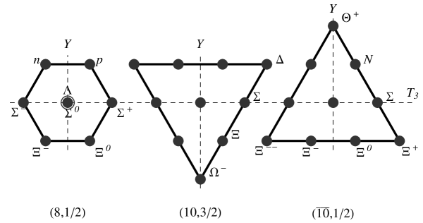
Figure 1.1: The lightest baryon multiplets: octet $\mathbf{8}$, decuplet $\mathbf{10}$ and hypothetic antidecuplet $\overline{\mathbf{10}}$.

More recently, Diakonov and Petrov with a technique based on light-cone baryon wave functions used in the present thesis have estimated more accurately the width and have found that it turns out to be $\sim 4$ MeV [76]. However, many approximations have been used such as non-relativistic limit and omission of some $5Q$ contributions (exchange diagrams). The authors expected that these have high probability to reduce further the width.

Exotic members of the antidecuplet can easily be recognized because their quantum numbers cannot be obtained from $3Q$ only. The problem is the identification of a nucleon resonance to a non-exotic or crypto-exotic member of this antidecuplet. It is then interesting to study the electromagnetic transition between octet and antidecuplet. From simple flavor $SU(3)$ symmetry considerations, the existence of antidecuplet would imply a sizeable breaking of isospin symmetry in the excitation of an octet nucleon into an antidecuplet nucleon. The magnetic transition between octet proton and crypto-exotic proton should be suppressed compared to the neutron case [77].

Candidates for the nucleon-like members of the antidecuplet have recently been discussed in the literature. The Partial Wave Analysis (PWA) of pion-nucleon scattering presented two candidates for $N_{\mathbf{\overline{10}}}$ with masses 1680 MeV and 1730 MeV [78]. Experimental evidence for a new nucleon resonance with mass near 1670 MeV has recently been obtained in the $\eta$ photoproduction on nucleon by the GRAAL collaboration [79]. A resonance peak is seen in the $\gamma n\to n\eta$ and is absent in the $\gamma p\to p\eta$ process. This resonance structure has a narrow width $\Gamma_{N^{*}\to\eta N}\simeq 40$ MeV. When the Fermi-motion corrections are taken into account the width may become even narrower $\Gamma_{N^{*}\to\eta N}\simeq 10$ MeV [80]. Such a narrow width naturally reminds pentaquark baryons. Even more recently the Tokohu LNS [81] and CB/TAPS@ELSA [82] reported $\eta$ photoproduction from the deuteron target and concluded on the same asymmetry.

The question of pentaquark is a very intriguing and confusing one. The predicted pentaquarks have very special properties such as unusual small width and large isospin breaking of nucleon photoexcitation. On the experimental side the situation is far from being clear and simple. While part of the original positive sightings have been refuted by further more accurate experiments, some striking positive signals persist and cannot be a priori understood as statistical fluctuations. Further experiments are therefore needed. Finally, let us emphasize that even if the existence of pentaquark is not confirmed we will have learned much on the problem of experimental resolution, techniques allowing one to detect a narrow resonance, validity of many theoretical assumptions, …On a more theoretical side, the absence of the predicted pentaquark will probably and definitely invalidate the rigid rotator quantization scheme for exotic states. Pentaquarks with narrow width may simply not exist. There can be however pentaquarks with very large width or with masses in a completely different range. There could also be no $5Q$ state at all but this would need some restriction due to QCD not known hitherto.

1.4 Motivations and Plan of the thesis

As we have seen understanding the baryon structure is still an open and challenging problem. The correct low-energy QCD model should in principle at the same time explain experimental data on baryon structure and properties, predict the unmeasured ones in a reliable manner, incorporate all relevant degrees of freedom, relate cleanly constituent and current quarks, be in some sense directly derived from QCD, …No present model fulfills all these requirements. That much is not in fact expected from models. We hope at least that they deal with the relevant degrees of freedom, reproduce the correct dynamics leading to the observed baryon structure and properties and of course give reliable predictions.

Many questions both on the experimental and theoretical sides have to be answered. Part of them have been shortly discussed in the present introduction because they are related to the results of our studies in the context of this thesis. Later they will be discussed a bit further but without pretending to be complete and exhaust the topics. For the interested reader many references to papers, reviews and lectures are given throughout the text.

The Chiral Quark-Soliton Model ($\chi$QSM) is among the most successful models in describing low-energy QCD. Recently it has been formulated on the light cone [76, 83] where the concept of wave function is well defined. The basic formula have been derived and the general technique developed. Then the axial decay constant of the nucleon and the pentaquark width have been investigated in the non-relativistic limit up to the $5Q$ Fock component.

The aim of the present thesis was to further explore this new approach to the model. One part of the work has been devoted to the estimation of corrections coming from previously neglected diagrams, relativity (quark angular momentum) and higher Fock components. The second part has been devoted to study in details light baryon properties and structure, extract the individual contributions due to each quark flavor and separate the valence contributions from the sea contributions. Let us stress that in this thesis we have performed only ab initio calculations, no fit to experimental data has been made.

This work is very interesting for many reasons. First of all, as mentioned earlier, this is a detailed study of baryon structure and properties in terms of valence, sea and flavor contributions. The values obtained are compared with the present experimental knowledge and many predictions for the unmeasured baryon properties are given. Due to the approximations specific to the approach and the model all the predictions should not be considered as quantitatively reliable but at least give some qualitative information. This work is also interesting since we have estimated the impact of many effects on the observables: quark angular momentum, quark-antiquark pairs, …This allows one to emphasize the importance and role of each degree of freedom.

The approach to $\chi$QSM we used is based on light-cone techniques. In Chapter 2 we give a short introduction to the light-cone approach. We remind why the light cone is appealing when describing baryons and how they are studied usually in light-cone models.

Then in Chapter 3 we give a short introduction to $\chi$QSM. The general baryon wave function is presented and all quantities needed in this thesis are defined and explicit expressions are given. The general technique for extracting baryon observables is also presented.

Our whole work has been done in the flavor $SU(3)$ limit. Before presenting the results obtained we discuss the implication of this symmetry on observables, introduce the parametrization used in the results and compare with the non-relativistic $SU(6)$ symmetry of the usual CQM in Chapter 4.

In Chapters 5, 6, 7 and 8 we collect our results for normalizations, vector, axial and tensor charges, and magnetic moments of all lightest baryon multiplets (octet, decuplet and antidecuplet). They are discussed and compared with the present experimental data. Part of these results have already been published [84] or submitted on the web [85, 86] waiting for publication. The remaining results (especially concerning magnetic moments) are collected in other papers in preparation [87].

We conclude this work in Chapter 9. We remind the important points and results of the thesis and give tracks for further studies.

We join to this work two appendices. The first one contains all the group integrals needed and explains how they can be obtained. The second one gives general tools for simplifying the problem of contracting the creation-annihilation operators leading to the identification and weight of the diagrams involved in a given Fock sector.

Chapter 2 Light-cone approach

2.1 Forms of dynamics

Particle physics needs a synthesis of special relativity and quantum mechanics. A quantum treatment is obvious since particle physics plays at scales several order of magnitude smaller than in atomic physics. These scales also require a relativistic formulation. Let us consider for example a typical hadronic scale of 1 fm which corresponds to momenta of the order $p\sim\hbar c/1$ fm $\simeq 200$ MeV. For particles with masses $M\lesssim 1$ GeV this implies sizable velocities $v\simeq p/M\gtrsim 0.2$ c and thus non-negligible relativistic effects.

A relativistic quantum mechanics requires the state vectors of a system to transform according to a unitary representation of the Poincaré group. The subgroup of continuous transformations, called the proper group, has ten generators satisfying a set of commutation relations called the proper Poincaré algebra.

A state vector $|t\rangle$ describes the system at a given “time” $t$. The evolution in “time” of is driven by the Hamiltonian $H$ operator of the system. As defined by Dirac [88], the Hamiltonian $H$ is that operator whose action on the state vector $|t\rangle$ of a physical system has the same effect as taking the partial derivative with respect to time $t$

$$H|t\rangle=i\frac{\partial}{\partial t}|t\rangle.$$ (2.1)

Its expectation value $\langle t|H|t\rangle$ is a constant of motion and is called “energy” of the system.

Time and space are however not separate issues. In a covariant theory they are only different aspects of the four-dimensional space-time. These concepts of space and time can be generalized in an operational sense. One can define “space” as that hypersurface in four-space on which one chooses the initial field configurations in accord with microcausality, i.e. a light emitted from any point on the hypersurface must not cross the hypersurface. The remaining fourth coordinate can be thought as being normal to that hypersurface and understood as “time”. There are many possible parametrizations or foliation of space-time. A change in parametrization $\tilde{x}(x)$ implies a change in metric in order to conserve the arc length $\mathrm{d}s^{2}$. This means that the covariant $x_{\mu}$ and contravariant components $x^{\mu}$ can be quite different and can have rather different interpretations.

We have then a certain freedom in describing the dynamics of a system. One should however exclude all parametrizations accessible by a Lorentz transformation. This limits considerably the freedom. Following Dirac [89] there are basically three different parametrizations or “forms” of dynamics: instant, front and point forms. They cannot be mapped on each other by a Lorentz transformation. They differ by the hypersurface $\Sigma$ in Minkowski four-space on which the initial conditions of the fields are given. To characterize the state of the system unambiguously, $\Sigma$ must intersect every world-line once and only once. One has then correspondingly different “times”. The instant form is the most familiar one with its hypersurface $\Sigma$ given at instant time $x^{0}=t=0$. In the front form the hypersurface $\Sigma$ is a tangent plane to the light cone defined at the light-cone time $x^{+}=(t+z)/\sqrt{2}=0$. There seems here to be problems with microcausality. Note however that a signal carrying information moves with the group velocity always smaller than phase velocity $c=1$. Thus if no information is carried by the signal, points on the light cone cannot communicate. In the point form the time-like coordinate is identified with the eigentime of the physical system and the hypersurface has a hyperboloid shape. In principle all these three forms yield the same physical results since physics should not depend on how we parametrize space-time. The choice of the form depends on the amount of work needed to solve the physical problem. Let us note that in the non-relativistic limit $c\to\infty$ only one foliation is possible, the instant form and the absolute time is Galilean. This is due to the fact that particles can have any velocity and thus any slope of the hypersurface can be obtained by Lorentz boost.

Among the ten generators of the Poincaré algebra, there are some that map $\Sigma$ into itself, not affecting the time evolution. They form the so-called stability subgroup and are referred to as kinematical generators. The others drive the evolution of the system and contain the entire dynamics. They are called dynamical generators or Hamiltonians.

The generic four-vector $A^{\mu}$ is written in Cartesian contravariant components as

$$A^{\mu}=(A^{0},A^{1},A^{2},A^{3})=(A^{0},\mathbf{A}).$$ (2.2)

Using Kogut and Soper convention, the light-cone components are defined as

$$A^{\mu}=(A^{+},\mathbf{A}_{\perp},A^{-}),\qquad\textrm{where }A^{\pm}=\frac{1}{\sqrt{2}}\,(A^{0}\pm A^{3}).$$ (2.3)

The norm of this four-vector is then given by

$$A^{2}=(A^{0})^{2}-\mathbf{A}^{2}=2A^{+}A^{-}-\mathbf{A}_{\perp}^{2}$$ (2.4)

and the scalar product of two four-vectors $A^{\mu}$ and $B^{\mu}$ by

$$A\cdot B=A^{0}B^{0}-\mathbf{A}\cdot\mathbf{B}=A^{+}B^{-}+A^{-}B^{+}-\mathbf{A}_{\perp}\cdot\mathbf{B}_{\perp}.$$ (2.5)

In the usual instant form the Hamiltonian operator $P_{0}$ is a constant of motion which acts as the displacement operator in instant time $x^{0}\equiv t$. In the light-cone approach or front form the Hamiltonian operator $P_{+}$ is a constant of motion which acts as the displacement operator in light-cone time $x^{+}\equiv(t+z)/\sqrt{2}$. Let emphasize that $\partial_{+}=\partial^{-}$ is a time-like derivative $\partial/\partial x^{+}=\partial/\partial x_{-}$ while $\partial_{-}=\partial^{+}$ is a space-like derivative $\partial/\partial x^{-}=\partial/\partial x_{+}$. Correspondingly $P_{+}=P^{-}$ is the Hamiltonian while $P_{-}=P^{+}$ is the longitudinal space-like momentum.

2.2 Advantages of the light-cone approach

Representations of the Poincaré group are labeled by eigenvalues of two Casimir operator $P^{2}$ and $W^{2}$. $P^{\mu}$ is the energy-momentum operator, $W^{\mu}$ is the Pauli-Lubanski operator [90] constructed from $P^{\mu}$ and the angular-momentum operator $M^{\mu\nu}$

$$W^{\mu}=-\frac{1}{2}\,\epsilon^{\mu\nu\rho\sigma}M_{\nu\rho}P_{\sigma}.$$ (2.6)

Their eigenvalues are respectively $m^{2}$ and $-m^{2}s(s+1)$ with $m$ the mass and $s$ the spin the particle. The states of a Dirac particle $s=1/2$ are eigenvectors of $P^{\mu}$ and polarization operator $\Pi\equiv-W\cdot s/m$

$$P^{\mu}|p,s\rangle = p^{\mu}|p,s\rangle,$$ (2.7)

$$-\frac{W\cdot s}{m}\,|p,s\rangle = \pm\frac{1}{2}\,|p,s\rangle$$ (2.8)

where $s^{\mu}$ is the spin (or polarization) vector of the particle with properties

$$s^{2}=-1,\qquad s\cdot p=0.$$ (2.9)

It can be written in general as

$$s^{\mu}=\left(\frac{\mathbf{p}\cdot\mathbf{n}}{m},\mathbf{n}+\frac{(\mathbf{p}\cdot\mathbf{n})\mathbf{p}}{m(m+p^{0})}\right)$$ (2.10)

where $\mathbf{n}$ is a unit vector identifying a generic space direction.

Since the Lagrangian of a system is frame-independent there must be ten conserved current corresponding to the ten Poincaré generators. Integrating these currents over a three-dimensional hypersurface of a hypersphere, embedded in the four-dimensional space-time, generates conserved charges. The proper Poincaré group has then ten conserved charges or constants of motion: the four components of the energy momentum tensor $P^{\mu}$ and the six components of the boost-angular momentum tensor $M^{\mu\nu}$. These ten constants of motion are observables and are thus hermitian operators with real eigenvalues. It is therefore advantageous to construct representations in which these constants of motion are diagonal. Unfortunately one cannot diagonalize all the ten simultaneously because they do not commute.

In the usual instant form dynamics the initial conditions are set at some instant of time and the hypersurfaces $\Sigma$ are flat three-dimensional surfaces only containing directions that lie outside the light cone. The generators of rotations and space translations leave the instant invariant, i.e. do not affect the dynamics. There are then six generators constituting the kinematical subgroup in the instant form: three momentum $P_{i}$ and three angular momentum generators $J_{i}=\frac{1}{2}\,\epsilon_{ijk}M_{jk}$. The remaining four generators are dynamical and therefore involve interaction: three boost $K_{i}=M_{i0}$ and one time-translation generators $P_{0}$.

In the front form dynamics one considers instead three-dimensional surfaces in space-time formed by a plane-wave front advancing at the velocity of light, e.g. $x^{+}=0$. In this case seven generators are kinematical $P_{1},P_{2},P_{-},M_{12},M_{+-},M_{1-},M_{2-}$. The three remaining ones $P_{+},M_{1+},M_{2+}$ are then dynamical. This corresponds in fact to best one can do [89]. One cannot diagonalize simultaneously more than seven Poincaré generators. Components of the energy-momentum operator are easily interpreted as generators of space $P_{1},P_{2},P_{-}$ and time translations $P_{+}$. Kogut and Soper [91] have written the components of the angular momentum operator in terms of boosts and angular momenta. They introduced the transversal vector $\mathbf{B}_{\perp}$

$$B_{1}=M_{1-}=\frac{1}{\sqrt{2}}\,(K_{1}+J_{2}),\qquad B_{2}=M_{2-}=\frac{1}{\sqrt{2}}\,(K_{2}-J_{1}).$$ (2.11)

They are kinematical and boost the system in the $x$ and $y$ direction respectively. The other kinematical operators $M_{12}=J_{3}$ and $M_{+-}=K_{3}$ rotate the system in the $x$-$y$ plane and boost it in the longitudinal direction respectively. The remaining dynamical operators are combined in a transversal angular-momentum vector $\mathbf{S}_{\perp}$

$$S_{1}=M_{1+}=\frac{1}{\sqrt{2}}\,(K_{1}-J_{2}),\qquad S_{2}=M_{2+}=\frac{1}{\sqrt{2}}\,(K_{2}+J_{1}).$$ (2.12)

Light-cone calculations for relativistic CQM are convenient as they allow to boost quark wave functions independently of the details of the interaction. Unlike the traditional instant form Hamiltonian formalism where the internal and center-of-mass motion of relativistic interacting particles cannot be separated in principle, the light-cone Hamiltonian formalism can be formulated without reference to a specific Lorentz frame. The drawback is however that the construction of states with good total angular momentum becomes interaction dependent. Except for the free theory, it is very hard to write down states with good angular momentum as diagonalizing $\mathbf{L}^{2}$ is as difficult as solving the Schrödinger equation. This is the notorious problem of angular momentum of the light-cone approach [93].

The useful concept of wave function borrowed from non-relativistic quantum mechanics is not well defined in instant form since the particle number of a state is neither bounded nor fixed. Quark-antiquark pairs are constantly popping in and out the vacuum. This means that even the ground state is complicated. One of biggest advantages of the front form is that the vacuum structure is much simpler. In many cases the vacuum state of the free Hamiltonian is also an eigenstate of the full light-cone Hamiltonian. Contrary to $P_{z}$ the operator $P^{+}$ is positive, having only positive eigenvalues. Each Fock state is eigenstate of the operators $P^{+}$ and $\mathbf{P}_{\perp}$. The eigenvalues are

$$\mathbf{P}_{\perp}=\sum_{i=1}^{n}\mathbf{p}_{\perp i},\qquad P^{+}=\sum_{i=1}^{n}p^{+}_{i}$$ (2.13)

with $p^{+}_{i}>0$ for massive quanta, $n$ being the number of particles in the Fock state. The vacuum has eigenvalue 0, i.e. $\mathbf{P}_{\perp}|0\rangle=\mathbf{0}$ and $P^{+}|0\rangle=0$. The restriction $p^{+}_{i}>0$ for massive quanta is the key difference between light-cone and ordinary equal-time quantization. In the latter the state of a parton is specified by its ordinary three-momentum $\mathbf{p}$. Since each component of the momentum can be either positive or negative there exists an infinite number of Fock states with zero total momentum. The physical vacuum $|\Omega\rangle$ is thus complicated. In the former particles have non-zero longitudinal momentum and the vacuum is identified to the zero-particle state $|\Omega\rangle=|0\rangle$.

The Fock expansion constructed on this vacuum provides thus a complete relativistic many-particle basis for the baryon states. This means that all constituents are directly related to the baryon state and not do disconnected vacuum fluctuations. The concept of wave function is then well defined on the light cone. The light-cone wave functions are frame independent and can be expressed by means of relative coordinates only because the boosts are kinematical. For example, Lorentz boost in the third direction is diagonal. Light-cone time and space do not get mixed but are just rescaled. Since $p^{+}_{i}>0$ and $P^{+}>0$ one can define boost-invariant longitudinal momentum fractions $z_{i}=p^{+}_{i}/P^{+}$ with $0<z_{i}<1$. In the intrinsic frame $\mathbf{P}_{\perp}=\mathbf{0}$ we have the constraints

$$\sum_{i=1}^{n}z_{i}=1,\qquad\sum_{i=1}^{n}\mathbf{p}_{\perp i}=\mathbf{0}.$$ (2.14)

These light-cone wave functions are very important and useful objects as they encode hadronic properties. In the context of QCD their relevance relies on the concept of factorization. Processes with hadrons at sufficiently high energy/momentum transfer can be divided into two parts: a hard part which can be calculated according to perturbative QCD and a soft part usually encoded in soft functions, parton distributions, fragmentation functions, …This soft part can in principle be expressed in terms of light-cone wave functions. For example PDF are forward matrix of non-local operator and can be obtained by squaring the wave function and integrating over some transverse momenta. With electromagnetic probes one has

$$f(x)\propto\int\mathrm{d}\lambda\,e^{i\lambda x}\langle P|\bar{\psi}(0)\gamma_{\mu}\psi(\lambda)|P\rangle\sim\int\mathrm{d}\mathbf{k}_{\perp}\,\psi^{\dagger}(x,\mathbf{k}_{\perp})\,\psi(x,\mathbf{k}_{\perp}).$$ (2.15)

Form factors (FF) are off-forward matrix elements of local operator and can be obtained from an overlap of light-cone wave functions

$$F(Q^{2})\propto\langle P^{\prime}|\bar{\psi}(0)\gamma_{\mu}\psi(0)|P\rangle\sim\int_{-1}^{1}\mathrm{d}x\int\mathrm{d}\mathbf{k}_{\perp}\,\psi^{\dagger}(x,\mathbf{k}_{\perp}+\mathbf{Q}_{\perp}/2)\,\psi(x,\mathbf{k}_{\perp}-\mathbf{Q}_{\perp}/2).$$ (2.16)

Generalized Parton Distributions (GPD) provide a natural interpolation between PDF and FF and are relevant in processes like Deeply Virtual Compton Scattering (DVCS) and hard meson production [94]. They are off-forward matrix elements of non-local operator and can also be easily presented in terms of light-cone wave functions [95]

$$GPD(x,\xi,Q^{2})\propto\int\mathrm{d}\lambda\,e^{i\lambda x}\langle P^{\prime}|\bar{\psi}(-\lambda/2)\gamma_{\mu}\psi(\lambda/2)|P\rangle\sim\int\mathrm{d}\mathbf{k}_{\perp}\,\psi^{\dagger}(x+\xi,\mathbf{k}_{\perp}+\mathbf{Q}_{\perp}/2)\,\psi(x-\xi,\mathbf{k}_{\perp}-\mathbf{Q}_{\perp}/2).$$ (2.17)

The light-cone calculation of nucleon form factors has been pioneered by Berestetsky and Terentev [96] and more recently developed by Chung and Coester [97]. Form factors are generally constructed from hadronic matrix elements of the current $\langle P+q|j^{\mu}(0)|P\rangle$. In the interaction picture one can identify the fully interacting Heisenberg current $J^{\mu}$ with the free current $j^{\mu}$ at the space-time point $x^{\mu}=0$. The computation of these hadronic matrix elements is greatly simplified in the so-called Drell-Yan-West (DYW) frame [98], i.e. in the limit $q^{+}=0$ where $q$ is the light-cone longitudinal transfer momentum. Matrix elements of the $+$ component of the current are diagonal in particle number $n^{\prime}=n$, i.e. the transitions between Fock states with different particle numbers are vanishing. The current can neither create nor annihilate quark-antiquark pairs. Such a simplification can be seen using projectors on “good” and “bad” components of a Dirac four-spinor. The operator $\mathcal{P}_{+}=\gamma^{-}\gamma^{+}/2$ projects the four-component Dirac spinor $\psi$ onto the two-dimensional subspace of “good” light-cone components which are canonically independent fields [91]. Likewise $\mathcal{P}^{-}=\gamma^{+}\gamma^{-}/2$ projects on the two-dimensional subspace of “bad” light-cone components which are interaction dependent fields and should not enter at leading twist.

Finally, instant form has also a practical disadvantage. For example, consider the wave function of an atom with $n$ electrons. An experiment which specifies the initial wave function would require simultaneous measurement of the position of all the bounded electrons. In contrast, the initial wave function at fixed light-cone time only requires an experiment which scatters one plane-wave laser beam since the signal reaches each of the $n$ electrons at the same light-cone time.

2.3 Light cone v.s. Infinite Momentum Frame

Dirac’s legacy has been forgotten and re-invented many times with other names. The Infinite Momentum Frame (IMF) first appeared in the work of Fubini and Furlan [99] in connection with current algebra as the limit of a reference frame moving with almost the speed of light. Weinberg [100] considered the infinite-momentum limit of old-fashioned perturbation diagrams for scalar meson theories and showed that the vacuum structure of these theories simplified in this limit. Later, Susskind [101] showed that the infinities which occur among the generators of the Poincaré group when they are boosted in the IMF can be scaled or substracted out consistently. The result is essentially a change in variables. With these new variables he drew the attention to the (two-dimensional) Galilean subgroup of the Poincaré group. Bardakci and Halpern [102] further analyzed the structure of theories in IMF. They viewed the infinite-momentum limit as a change of variables from the laboratory time $t$ and space coordinate $z$ to a new “time” $\tau=(t+z)/\sqrt{2}$ and a new “space” $\zeta=(t-z)/\sqrt{2}$. Kogut and Soper [91] have examined the formal foundations of Quantum ElectroDynamics (QED) in the IMF. Finally Drell and others [98, 103] have recognized that the formalism could serve as kind of natural tool for formulating the quark-parton model.

Let us consider two particles with three-momenta $\mathbf{p}_{1}$ and $\mathbf{p}_{2}$ and use the variables $\mathbf{P}=(\mathbf{p}_{1}+\mathbf{p}_{2})/2$ and $\mathbf{q}=\mathbf{p}_{2}-\mathbf{p}_{1}$. The IMF prescription is to take the limit $|\mathbf{P}|\to\infty$ and impose the condition $\mathbf{P}\cdot\mathbf{q}=0$, i.e. momentum transfer has to be orthogonal to the (very large) mean momentum which guarantees that the momentum transfer has no time component [104]. This prescription introduces from the outside an infinite factor in the covariant normalization for the physical states

$$\langle\mathbf{p}_{2}|\mathbf{p}_{1}\rangle=(2\pi)^{3}2E\,\delta^{(3)}(\mathbf{p}_{1}-\mathbf{p}_{2})\longrightarrow(2\pi)^{3}2|\mathbf{P}|\,\delta^{(3)}(\mathbf{p}_{1}-\mathbf{p}_{2}).$$ (2.18)

Thus the “natural” $|\mathbf{P}|$ power in an expansion is actually reduced by one unit. Any vector $\mathbf{v}$ can be decomposed into a longitudinal component $\mathbf{v}_{L}$ which is along the direction of $\mathbf{P}$ and a transverse component $\mathbf{v}_{\perp}$ which is orthogonal to $\mathbf{P}$. Let us consider in the following that $\mathbf{P}$ defines the $z$ direction.

Currents can be decomposed into “good” and “bad” components referring to their behavior in the limit $P_{z}\to\infty$. The “good” components behave like $P_{z}$ while “bad” components are of order $\mathcal{O}(1)$. The scalar $S$, pseudoscalar $P$, vector $V_{\mu}$, axial vector $A_{\mu}$ and tensor $T_{\mu\nu}$ operators have the most immediate relevance in elementary particle physics. “Good” components correspond to free quarks. Creation-annihilation of quark-antiquark pairs are suppressed. On the contrary, “bad” components correspond to interacting quarks. Creation-annihilation of quark-antiquark pairs are important. In the IMF the “good” operators appeared to be $V_{0},V_{3},A_{0},A_{3},T_{0\perp},T_{3\perp}$ and the “bad” ones to be $S,P,V_{\perp},A_{\perp},T_{00},T_{03},T_{33},T_{\perp\perp^{\prime}}$. This means that it is simple to compute the zeroth and third components of the vector and axial vector current in the IMF. Moreover these zeroth and third components coincide in the leading order in $P_{z}$. On the contrary scalar and pseudoscalar currents as well as transverse components of the vector and axial-vector currents are difficult because the interaction is involved.

These features naturally remind the light-cone approach in the DYW frame. The light-cone and IMF approaches are indeed identified in the literature. For example one defines the light-cone wave function as the instant-form wave function boosted to the IMF [105]. However unboosting the wave function from IMF is generally impossible. For a qualitative picture, all the physical processes in the IMF become as slow as possible because of time dilatation in this system of reference. The investigation of the wave function is equivalent to make a snapshot of as system not spoiled by vacuum fluctuations. Note also that in the IMF, there is no distinction between the quark helicity and its spin projection $S_{z}$. That is why both these two terms will be used without distinction.

2.4 Standard model approach based on Melosh rotation

As we have just seen, light-cone wave functions are obtained by boosting the rest-frame wave function. The usual approach is to use a $3Q$ rest-frame wave function ideally fitted to the baryon spectrum. The spin $S$ of a particle is not Lorentz invariant. Only the total angular momentum $J=L+S$ is the meaningful quantity. Its decomposition into spin $S$ and orbital angular momentum $L$ depends on the reference frame. This means that boosting a particle induces a change in its spin orientation.

The conventional spin three-vector $\mathbf{s}$ of a moving particle with finite mass $m$ and four-momentum $p_{\mu}$ can be defined by transforming its Pauli-Lubanski four-vector $W_{\mu}$ to its rest frame via a rotationless Lorentz boost $L(p)$ which satisfies $L(p)p=(m,\mathbf{0})$. One has [106]

$$(0,\mathbf{s})=L(p)W/m.$$ (2.19)

Under an arbitrary Lorentz transformation $\Lambda$ a particle of spin $\mathbf{s}$ and four-momentum $p_{\mu}$ will be mapped onto the state of spin $\mathbf{s}^{\prime}$ and four-momentum $p^{\prime}_{\mu}$ given by

$$\mathbf{s}^{\prime}=\mathcal{R}_{W}(\Lambda,p)\mathbf{s},\qquad p^{\prime}=\Lambda p$$ (2.20)

where $\mathcal{R}_{W}(\Lambda,p)=L(\Lambda p)\Lambda L^{-1}(p)$ is a pure rotation known as Wigner rotation.

So when a baryon is boosted via a rotationless Lorentz transformation along its spin direction from the rest frame to a frame where it is moving, each quark will undergo a Wigner rotation. Specified to the spin-1/2 case the Wigner rotation reduces to the Melosh rotation [107]

$$\psi^{i}_{LC,\lambda}=\frac{[(m+z_{i}\mathcal{M})\mathbb{1}+i\mathbf{n}\cdot(\boldsymbol{\sigma}\times\mathbf{p}_{i})]^{\lambda^{\prime}}_{\lambda}}{\sqrt{(m+z_{i}\mathcal{M})^{2}+\mathbf{p}^{2}_{i\perp}}}\,\psi^{i}_{\lambda^{\prime}}$$ (2.21)

where $\mathbf{n}=(0,0,1)$. This transformation assures that the baryon is an eigenfunction of $J$ and $J_{z}$ in its rest frame [106]. This rotation transforms rest-frame quark states $\psi^{i}_{\lambda^{\prime}}$ into light-cone quark states $\psi^{i}_{LC,\lambda}$, with $i=1,2,3$. Here is the explicit expression for the Melosh rotated states

$$\psi^{i}_{LC,+} = \frac{(m_{q}+z_{i}\mathcal{M})\psi^{i}_{\uparrow}+p_{i}^{R}\psi^{i}_{\downarrow}}{\sqrt{(m_{q}+z_{i}\mathcal{M})^{2}+\mathbf{p}_{i\perp}^{2}}},$$ (2.22)

$$\psi^{i}_{LC,-} = \frac{-p_{i}^{L}\psi^{i}_{\uparrow}+(m_{q}+z_{i}\mathcal{M})\psi^{i}_{\downarrow}}{\sqrt{(m_{q}+z_{i}\mathcal{M})^{2}+\mathbf{p}_{i\perp}^{2}}}$$ (2.23)

where $p_{i}^{R,L}=p_{i}^{x}\pm ip_{i}^{y}$ and $\mathcal{M}$ is the invariant mass $\mathcal{M}^{2}=\sum_{i=1}^{3}(\mathbf{p}_{i}^{2}+m_{q}^{2})/z_{i}$ with the constraints $\sum_{i=1}^{3}z_{i}=0$ and $\sum_{i=1}^{3}\mathbf{p}_{i\perp}=0$. The internal transverse-momentum dependence of the light-cone wave function also affects its helicity structure [108]. The zero-binding limit $z_{i}\mathcal{M}\to p^{+}_{i}$ is not a justified approximation for QCD bound states. This rotation mixes the helicity states due to a nonzero transverse momentum $\mathbf{p}_{i\perp}$. The light-cone spinor with helicity $+$ corresponds to total angular momentum projection $J_{z}=1/2$ and is thus constructed from a spin $\uparrow$ state with orbital angular momentum $L_{z}=0$ and a spin $\downarrow$ state with orbital angular momentum $L_{z}=+1$ expressed by the factor $p^{R}$. Similarly the light-cone spinor with helicity $-$ corresponds to total angular momentum projection $J_{z}=-1/2$ and is thus constructed from a spin $\uparrow$ state with orbital angular momentum $L_{z}=-1$ expressed by the factor $p^{L}$ and a spin $\downarrow$ state with orbital angular momentum $L_{z}=0$. Note however that the general form of a light-cone wave function [109] must contain two functions

$$\psi^{\sigma}_{\sigma_{1}}=\chi^{\dagger}_{\sigma_{1}}\left(f_{1}+i\,\mathbf{n}\cdot\frac{(\boldsymbol{\sigma}\times\mathbf{p})}{|\mathbf{p}|}f_{2}\right)\chi^{\sigma}.$$ (2.24)

The additional $f_{2}$ term represents a separate dynamical contribution to be contrasted with the purely kinematical contribution of angular momentum from Melosh rotations.

For a review on the light-cone topic, see [110].

Chapter 3 The Chiral Quark-Soliton Model

3.1 Introduction

As mentioned in the thesis introduction we know that a realistic description of the nucleon should incorporate the Spontaneous Chiral Symmetry Breaking (SCSB). This idea is one of the basics of the Chiral Quark-Soliton Model ($\chi$QSM) and plays a dominant role in the dynamics of the nucleon bound state.

As in the Skyrme model, $\chi$QSM is essentially based on a $1/N_{C}$ expansion where $N_{C}$ is the number of colors in QCD. It is a general QCD theorem that at large $N_{C}$ the nucleon is heavy and can be viewed as a classical soliton [11]. While the dynamical realization given by the Skyrme model [111] is based on unrealistic effective chiral Lagrangian, a far more realistic one has been proposed later [112]. This NJL-type Lagrangian has been derived from the instanton model of the QCD vacuum which provides a natural mechanism of chiral symmetry breaking. Based on this Lagrangian, the $\chi$QSM model [113, 114] has been proposed and describes baryon properties better than the Skyrme model. For a recent status of this model see the reviews [115, 116]. Let us also mention that Generalized Parton Distributions (GPD) [117] have also recently been computed in the model at a low normalization point.

A distinguishable feature of $\chi$QSM as compared with many other effective models of baryons, like NQM or MIT bag model, is that it is field theoretical model which takes into account not only three valence quarks but also the whole Dirac sea as degrees of freedom. It is also almost the only effective model that can give reliable predictions for the quark and antiquark distribution functions of the nucleon satisfying the fundamental field theoretical restrictions like positivity of the antiquark distribution [119, 118]. $\chi$QSM is often seen as the interpolation between two drastically different pictures of the nucleon, namely the NQM where we have only valence quarks and Skyrme model where we have only the pion field.

An important difference between $\chi$QSM and the Chiral Quark Model ($\chi$QM) is that in the former a non-trivial topology is introduced which is crucial for stabilizing the soliton whereas in the latter the $\chi$QM fields are treated as a perturbation. $\chi$QSM differs also from the linear $\sigma$-model [120] in that no kinetic energy at tree level is associated to the chiral fields. Pions propagate only through quark loops. Furthermore quark loops induce many-quark interactions, see Fig. 3.1. Consequently the emerging picture is rather far from a simple one-pion exchange between the constituent quarks: non-linear effects in the pion field are not at all suppressed.

Figure 3.1: Picture of the nucleon arising from models based on non-linear chiral Lagrangians. Quarks (solid lines) interact via pion fields (dashed lines) which propagate through quark loops inducing many-quark interactions.

Note also that the chiral fields are effective degrees of freedom, totally equivalent to the quark-antiquark excitations of the Dirac sea (no problem of double counting) [83].

3.1.1 The effective action of $\chi$QSM

$\chi$QSM is assumed to mimic low-energy QCD thanks to an effective action describing constituent quarks with a momentum dependent dynamical mass $M(p)$ interacting with the scalar $\Sigma$ and pseudoscalar $\boldsymbol{\Pi}$ fields. The chiral circle condition $\Sigma^{2}+\boldsymbol{\Pi}^{2}=1$ is invoked. Due to its momentum dependence $M(p)$ serves as a form factor for the constituent quarks and provides also the effective theory with the UV cutoff. At the same time, it makes the theory non-local as one can see in the action

$$S_{\textrm{eff}}=\int\frac{\mathrm{d}^{4}p\,\mathrm{d}^{4}p^{\prime}}{(2\pi)^{8}}\,\bar{\psi}(p)\left[p\!\!\!/\,(2\pi)^{4}\delta^{(4)}(p-p^{\prime})-\sqrt{M(p)}(\Sigma(p-p^{\prime})+i\Pi(p-p^{\prime})\gamma_{5})\sqrt{M(p^{\prime})}\right]\psi(p^{\prime})$$ (3.1)

where $\psi$ and $\bar{\psi}$ are quark fields. This action has been originally derived in the instanton model of the QCD vacuum [112]. After reproducing masses and decay constants in the mesonic sector, the only free parameter left to be fixed in the baryonic sector is the constituent quark mass. The number of gluons is suppressed in the instanton vacuum by the parameter $(M\rho)^{2}\ll 1$ where $\rho$ is the instanton size, so gluons in this model do not participate in the formation of the nucleon wave function. Note that oppositely to the naive bag picture, this action (3.1) is fully relativistic and supports all general principles and sum rules for conserved quantities.

The form factors $\sqrt{M(p)}$ cut off momenta at some characteristic scale which corresponds in the instanton picture to the inverse average size of instantons $1/\bar{\rho}\approx 600$ MeV. One can then consider the scale of this model to be $Q^{2}_{0}\approx 0.36$ GeV². This means that in the range of quark momenta $p\ll 1/\bar{\rho}$ one can neglect the non-locality. We use the standard approach: the constituent quark mass is replaced by a constant $M=M(0)$ and we mimic the decreasing function $M(p)$ by the UV Pauli-Villars cutoff [118]

$$S_{\textrm{eff}}=\int\frac{\mathrm{d}^{4}p}{(2\pi)^{4}}\,\bar{\psi}(p)(p\!\!\!/-MU^{\gamma_{5}})\psi(p)$$ (3.2)

with $U^{\gamma_{5}}$ a $SU(3)$ matrix

$$U^{\gamma_{5}}=\left(\begin{array}[]{cc}U_{0}&0\\ 0&1\end{array}\right),\qquad U_{0}=e^{i\boldsymbol{\pi}\cdot\boldsymbol{\tau}\gamma_{5}}=e^{i\pi\gamma_{5}}$$ (3.3)

and $\tau^{a}$ the usual $SU(2)$ Pauli matrices.

In the following we expose the general technique from [76] allowing one to derive the (light-cone) baryon wave functions.

3.2 Explicit baryon wave function

In $\chi$QSM it is easy to define the baryon wave function in the rest frame. Indeed this model represents quarks in the Hartree approximation in the self-consistent pion field. The baryon is then described as $N_{C}$ valence quarks + Dirac sea in that self-consistent external field. It has been shown [83] that the wave function of the Dirac sea is the coherent exponential of the quark-antiquark pairs

$$|\Omega\rangle=\exp\left(\int(\mathrm{d}\mathbf{p})(\mathrm{d}\mathbf{p}^{\prime})\,a^{\dagger}(\mathbf{p})W(\mathbf{p},\mathbf{p}^{\prime})b^{\dagger}(\mathbf{p}^{\prime})\right)|\Omega_{0}\rangle$$ (3.4)

where $|\Omega_{0}\rangle$ is the vacuum of quarks and antiquarks $a,b\,|\Omega_{0}\rangle=0$, $\langle\Omega_{0}|\,a^{\dagger},b^{\dagger}=0$, $(\mathrm{d}\mathbf{p})=\mathrm{d}^{3}\mathbf{p}/(2\pi)^{3}$ and $W(\mathbf{p},\mathbf{p}^{\prime})$ is the quark Green function at equal times in the background $\Sigma,\boldsymbol{\Pi}$ fields [83, 121] (its explicit expression is given in Subsection 3.4).

The saddle-point or mean-field approximation is invoked to obtain the stationary pion field corresponding to the nucleon at rest. A mean field approach is usually justified by the large number of participants. For example, the Thomas-Fermi model of atoms is justified at large $Z$ [122]. For baryons, the number of colors $N_{C}$ has been used as such parameter [11]. Since $N_{C}=3$ in the real world, one can wonder how accurate is the mean-field approach. The chiral field experiences fluctuations about its mean-field value of the order of $1/N_{C}$. These are loop corrections which are further suppressed by factors of $1/2\pi$ yielding to corrections typically of the order of 10% which are simply ignored. In the mean-field approximation the chiral field is replaced by the following spherically-symmetric self-consistent field

$$\pi(\mathbf{r})=\mathbf{n}\cdot\boldsymbol{\tau}\,P(r),\qquad\mathbf{n}=\mathbf{r}/r.$$ (3.5)

We then have on the chiral circle $\Pi(\mathbf{r})=\mathbf{n}\cdot\boldsymbol{\tau}\sin P(r)$, $\Sigma(\mathbf{r})=\Sigma(r)=\cos P(r)$ with $P(r)$ being the profile function of the self-consistent field. The latter is fairly approximated by [113, 114] (see Fig. 3.3)

$$P(r)=2\arctan\left(\frac{r_{0}^{2}}{r^{2}}\right),\qquad r_{0}\approx\frac{0.8}{M},\qquad M\approx 345\textrm{ MeV}.$$ (3.6)

Consequently, in this approach, most of low-energy properties of light baryons follow from the shape of the mean chiral field in the classical baryon.

Such a chiral field creates a bound-state level for quarks, whose wave function $\psi_{\textrm{lev}}$ satisfies the static Dirac equation with eigenenergy $E_{\textrm{lev}}$ in the $K^{p}=0^{+}$ sector with $K=T+J$ [113, 120, 123]

$$\psi_{\textrm{lev}}(\mathbf{r})=\left(\begin{array}[]{c}\epsilon^{ji}h(r)\\ -i\epsilon^{jk}(\mathbf{n}\cdot\sigma)^{i}_{k}\,j(r)\end{array}\right),\qquad\left\{\begin{array}[]{c}h^{\prime}+h\,M\sin P-j(M\cos P+E_{\textrm{lev}})=0\\ j^{\prime}+2j/r-j\,M\sin P-h(M\cos P-E_{\textrm{lev}})=0\end{array}\right.$$ (3.7)

where $i=1,2=\uparrow,\downarrow$ and $j=1,2$ are respectively spin and isospin indices. Solving those equations with the self-consistent field (3.5) one finds that “valence” quarks are tightly bound ($E_{\textrm{lev}}=200$ MeV) along with a lower component $j(r)$ smaller than the upper one $h(r)$ (see Fig. 3.3).

Figure 3.2: Profile of the self-consistent chiral field $P(r)$ in light baryons. The horizontal axis unit is $r_{0}=0.8/M=0.46$ fm.

Figure 3.3: Upper $s$-wave component $h(r)$ (solid) and lower $p$-wave component $j(r)$ (dashed) of the bound-state quark level in light baryons. Each of the three valence quarks has energy $E_{\textrm{lev}}=200$ MeV. Horizontal axis has units of $1/M=0.57$ fm.

For the valence quark part of the baryon wave function it is sufficient to write the product of $N_{C}$ quark creation operators that fill in the discrete level [83]

$$\prod_{\textrm{color}=1}^{N_{C}}\int(\mathrm{d}\mathbf{p})F(\mathbf{p})a^{\dagger}(\mathbf{p})$$ (3.8)

where $F(\mathbf{p})$ is obtained by expanding and commuting $\psi_{\textrm{lev}}(\mathbf{p})$ with the coherent exponential (3.4)

$$F(\mathbf{p})=\int(\mathrm{d}\mathbf{p}^{\prime})\sqrt{\frac{M}{\epsilon^{\prime}s}}[\bar{u}(\mathbf{p})\gamma_{0}\psi_{\textrm{lev}}(\mathbf{p})(2\pi)^{3}\delta^{(3)}(\mathbf{p}-\mathbf{p}^{\prime})-W(\mathbf{p},\mathbf{p}^{\prime})\bar{v}(\mathbf{p}^{\prime})\gamma_{0}\psi_{\textrm{lev}}(-\mathbf{p}^{\prime})].$$ (3.9)

One can see from the second term that the distorted Dirac sea contributes to the one-quark wave function. For the plane-wave Dirac bispinor $u_{\sigma}(\mathbf{p})$ and $v_{\sigma}(\mathbf{p})$ we used the standard basis

$$u_{\sigma}(\mathbf{p})=\left(\begin{array}[]{c}\sqrt{\frac{\epsilon+M}{2M}}s_{\sigma}\\ \sqrt{\frac{\epsilon-M}{2M}}\frac{\mathbf{p}\cdot\sigma}{|\mathbf{p}|}s_{\sigma}\end{array}\right),\qquad v_{\sigma}(\mathbf{p})=\left(\begin{array}[]{c}\sqrt{\frac{\epsilon-M}{2M}}\frac{\mathbf{p}\cdot\sigma}{|\mathbf{p}|}s_{\sigma}\\ \sqrt{\frac{\epsilon+M}{2M}}s_{\sigma}\end{array}\right),\qquad\bar{u}^{\sigma^{\prime}}u_{\sigma}=\delta^{\sigma^{\prime}}_{\sigma}=-\bar{v}^{\sigma^{\prime}}v_{\sigma}$$ (3.10)

where $\epsilon=+\sqrt{\mathbf{p}^{2}+M^{2}}$ and $s_{\sigma}$ are two 2-component spinors normalized to unity

$$s_{1}=\left(\begin{array}[]{c}1\\ 0\end{array}\right),\qquad s_{2}=\left(\begin{array}[]{c}0\\ 1\end{array}\right).$$ (3.11)

The complete baryon wave function is then given by the product of the valence part (3.8) and the coherent exponential (3.4)

$$|\Psi_{B}\rangle=\prod_{\textrm{color}=1}^{N_{C}}\int(\mathrm{d}\mathbf{p})F(\mathbf{p})a^{\dagger}(\mathbf{p})\exp\left(\int(\mathrm{d}\mathbf{p})(\mathrm{d}\mathbf{p}^{\prime})\,a^{\dagger}(\mathbf{p})W(\mathbf{p},\mathbf{p}^{\prime})b^{\dagger}(\mathbf{p}^{\prime})\right)|\Omega_{0}\rangle.$$ (3.12)

We remind that the saddle-point of the self-consistent pion field is degenerate in global translations and global $SU(3)$ flavor rotations (the $SU(3)$-breaking strange mass can be treated perturbatively later). These zero modes must be handled with care. The result is that integrating over translations leads to momentum conservation which means that the sum of all quarks and antiquarks momenta have to be equal to the baryon momentum. As first pointed out by Witten [11] and then derived using different techniques by a number of authors [124], the quantization rule for the rotations of the mean chiral field in the ordinary and flavor spaces is such that the lowest baryon multiplets are the octet with spin 1/2 and the decuplet with spin 3/2 followed by the exotic antidecuplet with spin 1/2. All of those multiplets have same parity. The lowest baryons appear just as rotational excitations of the same mean chiral field (soliton). They are distinguished by their specific rotational wave functions given explicitly in Section 3.3. Let us note that in $\chi$QSM $\Theta^{+}$ pentaquark is light because it is not the sum of constituent quark masses but rather a collective excitation of the mean chiral field inside baryons.

Since rotations of the chiral field are not slow we integrate exactly over $SU(3)$ rotations $R$ in this thesis. This has to be contrasted with the usual slowly-rotating approach used in former studies of $\chi$QSM in the instant form. This leads to the projection of the flavor state of all quarks and antiquarks onto the spin-flavor state $B(R)$ specific to any particular baryon from the $\left({\bf 8},\frac{1}{2}^{+}\right)$, $\left({\bf 10},\frac{3}{2}^{+}\right)$ and $\left({\bf\overline{10}},\frac{1}{2}^{+}\right)$ multiplets.

If we restore color ($\alpha=1,2,3$), flavor ($f=1,2,3$), isospin ($j=1,2$) and spin ($\sigma=1,2$) indices, we obtain the following quark wave function of a particular baryon $B$ with spin projection $k$ [83, 121]

$$|\Psi_{k}(B)\rangle = \int\mathrm{d}R\,B_{k}^{*}(R)\epsilon^{\alpha_{1}\alpha_{2}\alpha_{3}}\prod_{n=1}^{3}\int(\mathrm{d}\mathbf{p}_{n})R_{j_{n}}^{f_{n}}F^{j_{n}\sigma_{n}}(\mathbf{p}_{n})a^{\dagger}_{\alpha_{n}f_{n}\sigma_{n}}(\mathbf{p}_{n})$$ (3.13)

$$\times \exp\left(\int(\mathrm{d}\mathbf{p})(\mathrm{d}\mathbf{p}^{\prime})a^{\dagger}_{\alpha f\sigma}(\mathbf{p})R^{f}_{j}W^{j\sigma}_{j^{\prime}\sigma^{\prime}}(\mathbf{p},\mathbf{p}^{\prime})R^{{\dagger}j^{\prime}}_{f^{\prime}}b^{{\dagger}\alpha f^{\prime}\sigma^{\prime}}(\mathbf{p}^{\prime})\right)|\Omega_{0}\rangle.$$

The three $a^{\dagger}$ create three valence quarks with the same wave function $F$ while the rest of $a^{\dagger}$’s, $b^{\dagger}$’s create any number of additional quark-antiquark pairs whose wave function is $W$. One can notice that the valence quarks are antisymmetric in color whereas additional quark-antiquark pairs are color singlets. One can obtain the spin-flavor structure of a particular baryon by projecting a general $QQQ+n\,Q\bar{Q}$ state onto the quantum numbers of the baryon under consideration. This projection is an integration over all spin-flavor rotations $R$ with the rotational wave function $B^{*}_{k}(R)$ unique for a given baryon.

Expanding the coherent exponential allows one to get the $3Q$, $5Q$, $7Q$, …wave functions of a particular baryon. Explicit expressions for the baryon rotational wave functions $B(R)$, the $Q\bar{Q}$ pair wave function in a baryon $W^{j\sigma}_{j^{\prime}\sigma^{\prime}}(\mathbf{p},\mathbf{p}^{\prime})$ and the valence wave function $F^{j\sigma}(\mathbf{p})$ are given in the next sections.

3.3 Baryon rotational wave functions

Baryon rotational wave functions are in general given by the $SU(3)$ Wigner finite-rotation matrices [125] and any particular projection can be obtained by a $SU(3)$ Clebsch-Gordan technique. In order to see the symmetries of the quark wave functions explicitly, we keep the expressions for $B(R)$ and integrate over the Haar measure $\int\mathrm{d}R$ in eq. (3.13).

The rotational $D$-functions for the $\left({\bf 8},\frac{1}{2}^{+}\right)$, $\left({\bf 10},\frac{3}{2}^{+}\right)$ and $\left({\bf\overline{10}},\frac{1}{2}^{+}\right)$ multiplets are listed below in terms of the product of the $R$ matrices. Since the projection onto a particular baryon in eq. (3.13) involves the conjugated rotational wave function, we list the latter one only. The unconjugated ones are easily obtained by hermitian conjugation.

3.3.1 The octet $\left({\bf 8},\frac{1}{2}^{+}\right)$

From the $SU(3)$ group point of view, the octet transforms as $(p,q)=(1,1)$, i.e. the rotational wave function can be composed of a quark (transforming as $R$) and an antiquark (transforming as $R^{\dagger}$). Then the (conjugated) rotational wave function of an octet baryon having spin index $k=1,2$ is

$$\left[D^{(8,\frac{1}{2})*}(R)\right]^{g}_{f,k}\sim\epsilon_{kl}R^{{\dagger}l}_{f}R^{g}_{3}.$$ (3.14)

The flavor part of this octet tensor $P^{g}_{f}$ represents the particles as follows

$$P^{3}_{1}=N^{+}_{8},\qquad P^{3}_{2}=N^{0}_{8},\qquad P^{2}_{1}=\Sigma^{+}_{8},\qquad P^{1}_{2}=\Sigma^{-}_{8},$$

$$P^{1}_{1}=\frac{1}{\sqrt{2}}\,\Sigma^{0}_{8}+\frac{1}{\sqrt{6}}\,\Lambda^{0}_{8},\qquad P^{2}_{2}=-\frac{1}{\sqrt{2}}\,\Sigma^{0}_{8}+\frac{1}{\sqrt{6}}\,\Lambda^{0}_{8},$$ (3.15)

$$P^{3}_{3}=-\sqrt{\frac{2}{3}}\,\Lambda^{0}_{8},\qquad P^{2}_{3}=\Xi^{0}_{8},\qquad P^{1}_{3}=-\Xi^{-}_{8}.$$

For example, the proton ($f=1,g=3$) and neutron ($f=2,g=3$) rotational wave functions are

$$p^{+*}_{k}(R)=\sqrt{8}\,\epsilon_{kl}R^{{\dagger}l}_{1}R^{3}_{3},\qquad n^{0*}_{k}(R)=\sqrt{8}\,\epsilon_{kl}R^{{\dagger}l}_{2}R^{3}_{3}.$$ (3.16)

3.3.2 The decuplet $\left({\bf 10},\frac{3}{2}^{+}\right)$

The decuplet transforms as $(p,q)=(3,0)$, i.e. the rotational wave function can be composed of three quarks. The rotational wave functions are then labeled by a triple flavor index $\{f_{1}f_{2}f_{3}\}$ symmetrized in flavor and by a triple spin index $\{k_{1}k_{2}k_{3}\}$ symmetrized in spin

$$\left[D^{(10,\frac{3}{2})*}(R)\right]_{\{f_{1}f_{2}f_{3}\}\{k_{1}k_{2}k_{3}\}}\sim\epsilon_{k^{\prime}_{1}k_{1}}\epsilon_{k^{\prime}_{2}k_{2}}\epsilon_{k^{\prime}_{3}k_{3}}R^{{\dagger}k^{\prime}_{1}}_{f_{1}}R^{{\dagger}k^{\prime}_{2}}_{f_{2}}R^{{\dagger}k^{\prime}_{3}}_{f_{3}}\Big{|}_{\textrm{sym in }\{f_{1}f_{2}f_{3}\}}.$$ (3.17)

The flavor part of this decuplet tensor $D_{f_{1}f_{2}f_{3}}$ represents the particles as follows

$$\begin{array}[]{llll}D_{111}=\sqrt{6}\,\Delta^{++}_{10},&D_{112}=\sqrt{2}\,\Delta^{+}_{10},&D_{122}=\sqrt{2}\,\Delta^{0}_{10},&D_{222}=\sqrt{6}\,\Delta^{-}_{10},\\ D_{113}=\sqrt{2}\,\Sigma^{+}_{10},&D_{123}=-\Sigma^{0}_{10},&D_{223}=-\sqrt{2}\,\Sigma^{-}_{10},&D_{133}=\sqrt{2}\,\Xi^{0}_{10},\\ &D_{233}=\sqrt{2}\,\Xi^{-}_{10},&D_{333}=-\sqrt{6}\,\Omega^{-}_{10}.&\end{array}$$ (3.18)

For example, the $\Delta^{++}$ with spin projection 3/2 ($f_{1}=1,f_{2}=1,f_{3}=1$) and $\Delta^{0}$ with spin projection 1/2 ($f_{1}=1,f_{2}=2,f_{3}=2$) rotational wave functions are

$$\Delta^{++*}_{\uparrow\uparrow\uparrow}(R)=\sqrt{10}\,R^{{\dagger}2}_{1}R^{{\dagger}2}_{1}R^{{\dagger}2}_{1},\qquad\Delta^{0*}_{\uparrow}(R)=\sqrt{10}\,R^{{\dagger}2}_{2}(2R^{{\dagger}2}_{1}R^{{\dagger}1}_{2}+R^{{\dagger}2}_{2}R^{{\dagger}1}_{1}).$$ (3.19)

3.3.3 The antidecuplet $\left({\bf\overline{10}},\frac{1}{2}^{+}\right)$

The antidecuplet transforms as $(p,q)=(0,3)$, i.e. the rotational wave function can be composed of three antiquarks. The rotational wave functions are then labeled by a triple flavor index $\{f_{1}f_{2}f_{3}\}$ symmetrized in flavor

$$\left[D^{(\overline{10},\frac{1}{2})*}(R)\right]^{\{f_{1}f_{2}f_{3}\}}_{k}\sim R^{f_{1}}_{3}R^{f_{2}}_{3}R^{f_{3}}_{k}\Big{|}_{\textrm{sym in }\{f_{1}f_{2}f_{3}\}}.$$ (3.20)

The flavor part of this antidecuplet tensor $T^{f_{1}f_{2}f_{3}}$ represents the particles as follows

$$\begin{array}[]{llll}T^{111}=\sqrt{6}\,\Xi^{--}_{\overline{10}},&T^{112}=-\sqrt{2}\,\Xi^{-}_{\overline{10}},&T^{122}=\sqrt{2}\,\Xi^{0}_{\overline{10}},&T^{222}=-\sqrt{6}\,\Xi^{+}_{\overline{10}},\\ T^{113}=\sqrt{2}\,\Sigma^{-}_{\overline{10}},&T^{123}=-\Sigma^{0}_{\overline{10}},&T^{223}=-\sqrt{2}\,\Sigma^{+}_{\overline{10}},&T^{133}=\sqrt{2}\,N^{0}_{\overline{10}},\\ &T^{233}=-\sqrt{2}\,N^{+}_{\overline{10}},&T^{333}=\sqrt{6}\,\Theta^{+}_{\overline{10}}.&\end{array}$$ (3.21)

For example, the $\Theta^{+}$ ($f_{1}=3,f_{2}=3,f_{3}=3$) and crypto-exotic neutron ($f_{1}=1,f_{2}=3,f_{3}=3$) rotational wave functions are

$$\Theta^{+*}_{k}(R)=\sqrt{30}\,R^{3}_{3}R^{3}_{3}R^{3}_{k},\qquad n^{0*}_{\overline{10},k}(R)=\sqrt{10}\,R^{3}_{3}(2R^{1}_{3}R^{3}_{k}+R^{3}_{3}R^{1}_{k}).$$ (3.22)

All examples of rotational wave functions above have been normalized in such a way that for any (but the same) spin projection we have

$$\int\mathrm{d}R\,B^{*}_{\textrm{spin}}(R)B^{\textrm{spin}}(R)=1,$$ (3.23)

the integral being zero for different spin projections. Note that rotational wave functions belonging to different baryons are also orthogonal. This can be easily checked using the group integrals in Appendix A. The particle representations (LABEL:Octet), (3.18) and (LABEL:Antidecuplet) have been found in [126].

3.4 Formulation in the Infinite Momentum Frame

As explained earlier the formulation in the IMF or equivalently on the light cone is very appealing. Thanks to the particularly simple structure of the vacuum the concept of wave function (borrowed from quantum mechanics) is well defined. By definition [105] a light-cone wave function is the wave function in the Infinite Momentum Frame, i.e. in the frame where the particle is travelling with almost the speed of light. Usually one cannot start with the instant form wave function and boost it to the IMF because boosts involve interaction. However as the effective chiral Lagrangian is relativistically invariant, we are guaranteed that there are infinitely many solutions of saddle-point equations of motion which describe the nucleon moving in some direction with speed $V$. The IMF is obtained when $V\to 1$. The corresponding pion field becomes time-dependent and can be obtained from the stationary field by a Lorentz transformation [83].

3.4.1 $Q\bar{Q}$ pair wave function

In [83, 121] it is explained that the pair wave function $W^{j\sigma}_{j^{\prime}\sigma^{\prime}}(\mathbf{p},\mathbf{p}^{\prime})$ is expressed by means of the finite-time quark Green function at equal times in the external static chiral field (3.5). The Fourier transforms of this chiral field will be needed

$$\Pi(\mathbf{q})^{j}_{j^{\prime}}=\int\mathrm{d}^{3}\mathbf{x}\,e^{-i\mathbf{q}\cdot\mathbf{x}}(\mathbf{n}\cdot\boldsymbol{\tau})^{j}_{j^{\prime}}\sin P(r),\qquad\Sigma(\mathbf{q})^{j}_{j^{\prime}}=\int\mathrm{d}^{3}\mathbf{x}\,e^{-i\mathbf{q}\cdot\mathbf{x}}(\cos P(r)-1)\delta^{j}_{j^{\prime}}$$ (3.24)

where $\Pi(\mathbf{q})$ is purely imaginary and odd and $\Sigma(\mathbf{q})$ is real and even. They can be rewritten as follows

$$\Pi(\mathbf{q})^{j}_{j^{\prime}}=i\,\frac{(\mathbf{q}\cdot\boldsymbol{\tau})^{j}_{j^{\prime}}}{|\mathbf{q}|}\,\Pi(q),\qquad\Pi(q)=\frac{4\pi}{q^{2}}\int_{0}^{\infty}\mathrm{d}r\,\sin P(r)\left(qr\cos qr-\sin qr\right)$$ (3.25)

$$\Sigma(\mathbf{q})^{j}_{j^{\prime}}=\delta^{j}_{j^{\prime}}\,\Sigma(q),\qquad\qquad\quad\Sigma(q)=\frac{4\pi}{q}\int_{0}^{\infty}\mathrm{d}r\,r\left(\cos P(r)-1\right)\sin qr$$ (3.26)

where the radial functions are depicted in Fig. 3.4.

Figure 3.4: The self-consistent pseudoscalar $-|\mathbf{q}|\Pi(\mathbf{q})$ (solid) and scalar $-|\mathbf{q}|\Sigma(\mathbf{q})$ (dashed) fields in baryons. The horizontal axis unit is $M$.

A simplified interpolating approximation for the pair wave function $W$ has also been derived and becomes exact in three limiting cases:

1. small pion field $P(r)$,

2. slowly varying $P(r)$ and

3. fast varying $P(r)$.

Since the model is relativistically invariant, this wave function can be translated to the infinite momentum frame (IMF). In this particular frame, the result is a function of the fractions of the baryon longitudinal momentum carried by the quark $z$ and antiquark $z^{\prime}$ of the pair and their transverse momenta $\mathbf{p}_{\perp}$, $\mathbf{p}^{\prime}_{\perp}$

$$W^{j\sigma}_{j^{\prime}\sigma^{\prime}}(z,\mathbf{p}_{\perp};z^{\prime},\mathbf{p}^{\prime}_{\perp})=\frac{M\mathcal{M}}{2\pi Z}\left\{\Sigma^{j}_{j^{\prime}}(\mathbf{q})[M(z^{\prime}-z)\tau_{3}+\mathbf{Q}_{\perp}\cdot\boldsymbol{\tau}_{\perp}]^{\sigma}_{\sigma^{\prime}}-i\Pi^{j}_{j^{\prime}}(\mathbf{q})[-M(z^{\prime}+z)\mathbb{1}+i\mathbf{Q}_{\perp}\times\boldsymbol{\tau}_{\perp}]^{\sigma}_{\sigma^{\prime}}\right\}$$ (3.27)

where $\mathbf{q}=((\mathbf{p}+\mathbf{p}^{\prime})_{\perp},(z+z^{\prime})\mathcal{M})$ is the three-momentum of the pair as a whole transferred from the background fields $\Sigma(\mathbf{q})$ and $\Pi(\mathbf{q})$, $\tau_{1,2,3}$ are Pauli matrices, $\mathcal{M}$ is the baryon mass and $M$ is the constituent quark mass. In order to simplify the notations we used

$$Z=\mathcal{M}^{2}zz^{\prime}(z+z^{\prime})+z(p^{\prime 2}_{\perp}+M^{2})+z^{\prime}(p^{2}_{\perp}+M^{2}),\qquad\mathbf{Q}_{\perp}=z\mathbf{p}^{\prime}_{\perp}-z^{\prime}\mathbf{p}_{\perp}.$$ (3.28)

This pair wave function $W$ is normalized in such a way that the creation-annihilation operators satisfy the following anticommutation relations

$$\{a^{\alpha_{1}f_{1}\sigma_{1}}(z_{1},\mathbf{p}_{1\perp}),a^{\dagger}_{\alpha_{2}f_{2}\sigma_{2}}(z_{2},\mathbf{p}_{2\perp})\}=\delta^{\alpha_{1}}_{\alpha_{2}}\delta^{f_{1}}_{f_{2}}\delta^{\sigma_{1}}_{\sigma_{2}}\delta(z_{1}-z_{2})(2\pi)^{2}\delta^{(2)}(\mathbf{p}_{1\perp}-\mathbf{p}_{2\perp})$$ (3.29)

and similarly for $b$, $b^{\dagger}$, the integrals over momenta being understood as $\int\mathrm{d}z\int\mathrm{d}^{2}\mathbf{p}_{\perp}/(2\pi)^{2}$.

A more compact form for this wave function can be obtained by means of the following two variables

$$y=\frac{z^{\prime}}{z+z^{\prime}},\qquad\mathcal{Q}_{\perp}=\frac{z\mathbf{p}^{\prime}_{\perp}-z^{\prime}\mathbf{p}_{\perp}}{z+z^{\prime}}.$$ (3.30)

The pair wave function then takes the form

$$W^{j,\sigma}_{j^{\prime}\sigma^{\prime}}(y,\mathbf{q},\mathcal{Q}_{\perp})=\frac{M\mathcal{M}}{2\pi}\frac{\Sigma^{j}_{j^{\prime}}(\mathbf{q})[M(2y-1)\tau_{3}+\mathcal{Q}_{\perp}\cdot\boldsymbol{\tau}_{\perp}]^{\sigma}_{\sigma^{\prime}}-i\Pi^{j}_{j^{\prime}}(\mathbf{q})[-M\mathbf{1}+i\mathcal{Q}_{\perp}\times\boldsymbol{\tau}_{\perp}]^{\sigma}_{\sigma^{\prime}}}{\mathcal{Q}^{2}_{\perp}+M^{2}+y(1-y)\mathbf{q}^{2}}.$$ (3.31)

3.4.2 Discrete-level wave function

We see from eq. (3.9) that the discrete-level wave function $F^{j\sigma}(\mathbf{p})=F^{j\sigma}_{\textrm{lev}}(\mathbf{p})+F^{j\sigma}_{\textrm{sea}}(\mathbf{p})$ is the sum of two parts: the one is directly the wave function of the valence level and the other is related to the change of the number of quarks at the discrete level due to the presence of the Dirac sea. I t is a relativistic effect and can be ignored in the non-relativistic limit ($E_{\textrm{lev}}\approx M$) together with the small $L=1$ lower component $j(r)$. Indeed, in the baryon rest frame $F^{j\sigma}_{\textrm{lev}}$ gives

$$F^{j\sigma}_{\textrm{lev}}=\epsilon^{j\sigma}\left(\sqrt{\frac{E_{\textrm{lev}}+M}{2E_{\textrm{lev}}}}h(p)+\sqrt{\frac{E_{\textrm{lev}}-M}{2E_{\textrm{lev}}}}j(p)\right)$$ (3.32)

where $h(p)$ and $j(p)$ are the Fourier transforms of the valence wave function, see Fig. 3.5

$$h(p) = \int\mathrm{d}^{3}\mathbf{x}\,e^{-i\mathbf{p}\cdot\mathbf{x}}h(r)=4\pi\int_{0}^{\infty}\mathrm{d}r\,r^{2}\frac{\sin pr}{pr}h(r),$$ (3.33)

$$j^{a}(p) = \int\mathrm{d}^{3}\mathbf{x}\,e^{-i\mathbf{p}\cdot\mathbf{x}}(-in^{a})j(r)=\frac{p^{a}}{|\mathbf{p}|}\,j(p),\qquad j(p)=\frac{4\pi}{p^{2}}\int_{0}^{\infty}\mathrm{d}r\,(pr\cos pr-\sin pr)j(r).$$ (3.34)

Figure 3.5: Fourier transforms of the upper $s$-wave component $h(p)$ (solid) and lower $p$-wave component $j(p)$ (dashed) of the bound-state quark level in light baryons. Horizontal axis has units of $M$.

In the non-relativistic limit the second term is double-suppressed: first due to the kinematical factor and second due to the smallness of the $L=1$ wave $j(r)$ compared to the $L=0$ wave $h(r)$.

Switching to the IMF one obtains [83, 121]

$$F^{j\sigma}_{\textrm{lev}}(z,\mathbf{p}_{\perp})=\sqrt{\frac{\mathcal{M}}{2\pi}}\left[\epsilon^{j\sigma}h(p)+(p_{z}\mathbb{1}+i\mathbf{p}_{\perp}\times\boldsymbol{\tau}_{\perp})^{\sigma}_{\sigma^{\prime}}\epsilon^{j\sigma^{\prime}}\frac{j(p)}{|\mathbf{p}|}\right]_{p_{z}=z\mathcal{M}-E_{\textrm{lev}}}.$$ (3.35)

As expected for a covariant light-cone wave function two distributions are involved $h$ and $j$, see eq. (2.24)

The “sea” part of the discrete-level wave function gives in the IMF

$$F^{j\sigma}_{\textrm{sea}}(z,\mathbf{p}_{\perp})=-\sqrt{\frac{\mathcal{M}}{2\pi}}\int\mathrm{d}z^{\prime}\frac{\mathrm{d}^{2}\mathbf{p}^{\prime}_{\perp}}{(2\pi)^{2}}\,W^{j\sigma}_{j^{\prime}\sigma^{\prime}}(z,\mathbf{p}_{\perp};z^{\prime},\mathbf{p}^{\prime}_{\perp})\,\epsilon^{j^{\prime}\sigma^{\prime\prime}}\left[(\tau_{3})^{\sigma^{\prime}}_{\sigma^{\prime\prime}}h(p^{\prime})-(\mathbf{p}^{\prime}\cdot\tau)^{\sigma^{\prime}}_{\sigma^{\prime\prime}}\frac{j(p^{\prime})}{|\mathbf{p}^{\prime}|}\right]_{p^{\prime}_{z}=z^{\prime}\mathcal{M}-E_{\textrm{lev}}}.$$ (3.36)

This sea part will be ignored in the present thesis. It is difficult to estimate its impact without an explicit computation.

In the work made by Diakonov and Petrov [76], the relativistic effects in the discrete-level wave function were neglected. One can then use only the first term in (3.35)

$$F^{j\sigma}(z,\mathbf{p}_{\perp})\approx\sqrt{\frac{\mathcal{M}}{2\pi}}\,\epsilon^{j\sigma}h(p)\big{|}_{p_{z}=z\mathcal{M}-E_{\textrm{lev}}}.$$ (3.37)

In the following the function $h(p)$ and $j(p)$ are understood with the condition $p_{z}=z\mathcal{M}-E_{\textrm{lev}}$.

3.5 Baryon Fock components

In a realistic picture baryons cannot be made of three (valence) quarks only. It has been soon realized that pions or quark-antiquark pairs are also present but the naive idea was that they can be in some sense integrated out and their effects encoded in valence quark non-trivial form factors. This idea was supported by the fact that axial decay constants and especially magnetic moments seem well described with three quarks only. However more recent experiments revealed the presence of hidden flavor in nucleons. Even though the number of strange quarks and antiquarks is the same, the strangeness contribution to nucleon spin and magnetic moment is non-zero. This indicates that the sea of quark-antiquarks or the pion cloud has to be somehow implemented explicitly in models.

In the present approach light baryons are explicitly described as an infinite tower of Fock states thanks to the coherent exponential (3.4). The latter can then be expanded to obtain any baryon $nQ$ Fock component. In this thesis we have expanded the wave function up to the $7Q$ component. We will see that the higher is the Fock state the smaller is its contribution to observables.

3.5.1 $3Q$ component of baryons

We will show in this section how to derive systematically the $3Q$ component of the octet and decuplet baryons (antidecuplet baryons have no such component). On the top of that we will also show that they become in the non-relativistic limit similar to the well-known $SU(6)$ wave functions of the constituent quark model.

An expansion of the coherent exponential gives access to all Fock components of the baryon wave function. Since we are interested in the present case only in the $3Q$ component, this coherent exponential is just ignored (since it has to be expanded to the zeroth order, i.e. $e^{\int\mathrm{d}\mathbf{p}\,\mathrm{d}\mathbf{p}^{\prime}W}\sim 1$). One can see from eq. (3.13) that the three valence quarks are rotated by the $SU(3)$ matrices $R^{f}_{j}$ where $f=1,2,3\equiv u,d,s$ is the flavor and $j=1,2$ is the isospin index. The projection of the $3Q$ state onto the quantum numbers of a specific baryon leads to the following group integral

$$T(B)^{f_{1}f_{2}f_{3}}_{j_{1}j_{2}j_{3},k}\equiv\int\mathrm{d}R\,B^{*}_{k}(R)R^{f_{1}}_{j_{1}}R^{f_{2}}_{j_{2}}R^{f_{3}}_{j_{3}}.$$ (3.38)

The group integrals can be found in Appendix A. This tensor $T$ must be contracted with the three discrete-level wave functions to obtain the $3Q$ baryon wave function

$$F^{j_{1}\sigma_{1}}(p_{1})F^{j_{2}\sigma_{2}}(p_{2})F^{j_{3}\sigma_{3}}(p_{3}).$$ (3.39)

The wave function is schematically represented on Fig. 3.7.

Let us consider, for example, the non-relativistic $3Q$ wave function of the neutron in the coordinate space

$$(|n\rangle_{k})^{f_{1}f_{2}f_{3},\sigma_{1}\sigma_{2}\sigma_{3}}(\mathbf{r}_{1},\mathbf{r}_{2},\mathbf{r}_{3}) = \frac{\sqrt{8}}{24}\,\epsilon^{f_{1}f_{2}}\epsilon^{\sigma_{1}\sigma_{2}}\delta^{f_{3}}_{2}\delta^{\sigma_{3}}_{k}h(r_{1})h(r_{2})h(r_{3})$$ (3.40)

$$+$$ cyclic permutations of (1,2,3)

times the antisymmetric tensor $\epsilon^{\alpha_{1}\alpha_{2}\alpha_{3}}$ in color. This equation means that in the non-relativistic $3Q$ picture the whole neutron spin $k$ is carried by a $d$ quark $\delta^{f_{3}}_{2}\delta^{\sigma_{3}}_{k}$ while the $ud$ pair is in the spin- and isospin-zero combination $\epsilon^{f_{1}f_{2}}\epsilon^{\sigma_{1}\sigma_{2}}$. This is similar to the better known non-relativistic $SU(6)$ wave function of the neutron

$$|n\uparrow\rangle = 2|d\uparrow(r_{1})\rangle|d\uparrow(r_{2})\rangle|u\downarrow(r_{3})\rangle-|d\uparrow(r_{1})\rangle|u\uparrow(r_{2})\rangle|d\downarrow(r_{3})\rangle-|u\uparrow(r_{1})\rangle|d\uparrow(r_{2})\rangle|d\downarrow(r_{3})\rangle$$ (3.41)

$$+ \textrm{ cyclic permutations of (1,2,3)}.$$

There are, of course, many relativistic corrections arising from the exact discrete-level wave function (3.35)+(3.36) and the additional quark-antiquark pairs, both effects being potentially not small.

Figure 3.6: Schematic representation of the $3Q$ component of baryon wave functions. The dark gray rectangle stands for the three discrete-level wave functions $F^{j_{i}\sigma_{i}}(\mathbf{p}_{i})$.

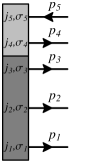
Figure 3.7: Schematic representation of the $5Q$ component of baryon wave functions. The light gray rectangle stands for the pair wave function $W^{j_{i}\sigma_{i}}_{j_{k}\sigma_{k}}(\mathbf{p}_{i},\mathbf{p}_{k})$ where the reversed arrow represents the antiquark.

3.5.2 $5Q$ component of baryons

The $5Q$ component of the baryon wave functions is obtained by expanding the coherent exponential (3.4) to the first order in the $Q\bar{Q}$ pair. The projection involves now along with the three $R$’s from the discrete level two additional matrices $R\,R^{\dagger}$ that rotate the quark-antiquark pair in the $SU(3)$ space

$$T(B)^{f_{1}f_{2}f_{3}f_{4},j_{5}}_{j_{1}j_{2}j_{3}j_{4},f_{5},k}\equiv\int\mathrm{d}R\,B^{*}_{k}(R)R^{f_{1}}_{j_{1}}R^{f_{2}}_{j_{2}}R^{f_{3}}_{j_{3}}\left(R^{f_{4}}_{j_{4}}R^{{\dagger}j_{5}}_{f_{5}}\right).$$ (3.42)

Components $i=1,2,3$ refer then to the valence part, $i=4$ to the quark of the sea and $i=5$ to the antiquark. One obtains the following $5Q$ component of the neutron wave function in the momentum space

$$(|n\rangle_{k})^{f_{1}f_{2}f_{3}f_{4},\sigma_{1}\sigma_{2}\sigma_{3}\sigma_{4}}_{f_{5},\sigma_{5}}(p_{1}\ldots p_{5}) = \frac{\sqrt{8}}{360}\,F^{j_{1}\sigma_{1}}(p_{1})F^{j_{2}\sigma_{2}}(p_{2})F^{j_{3}\sigma_{3}}(p_{3})W^{j_{4}\sigma_{4}}_{j_{5}\sigma_{5}}(p_{4},p_{5})$$ (3.43)

$$\times \epsilon_{k^{\prime}k}\left\{\epsilon^{f_{1}f_{2}}\epsilon_{j_{1}j_{2}}\left[\delta^{f_{3}}_{2}\delta^{f_{4}}_{f_{5}}\left(4\delta^{j_{5}}_{j_{4}}\delta^{k^{\prime}}_{j_{3}}-\delta^{j_{5}}_{j_{3}}\delta^{k^{\prime}}_{j_{4}}\right)+\delta^{f_{4}}_{2}\delta^{f_{3}}_{f_{5}}\left(4\delta^{j_{5}}_{j_{3}}\delta^{k^{\prime}}_{j_{4}}-\delta^{j_{5}}_{j_{4}}\delta^{k^{\prime}}_{j_{3}}\right)\right]\right.$$

$$+ \epsilon^{f_{1}f_{4}}\epsilon_{j_{1}j_{4}}\left[\delta^{f_{2}}_{2}\delta^{f_{3}}_{f_{5}}\left(4\delta^{j_{5}}_{j_{3}}\delta^{k^{\prime}}_{j_{2}}-\delta^{j_{5}}_{j_{2}}\delta^{k^{\prime}}_{j_{3}}\right)+\delta^{f_{3}}_{2}\delta^{f_{2}}_{f_{5}}\left(4\delta^{j_{5}}_{j_{2}}\delta^{k^{\prime}}_{j_{3}}-\delta^{j_{5}}_{j_{3}}\delta^{k^{\prime}}_{j_{2}}\right)\right]$$

$$+ \textrm{cyclic permutations of (1,2,3)}\Big{\}}.$$

The color degrees of freedom are not explicitly written but the three valence quarks (1,2,3) are still antisymmetric in color while the quark-antiquark pair (4,5) is a color singlet. The wave function is schematically represented on Fig. 3.7. Let us concentrate on the flavor part of this wave function. The quark-antiquark pair introduces explicitly the hidden strange flavor thanks to the terms like $\delta^{f_{4}}_{f_{5}}$ for the particular component $f_{4}=f_{5}=3\equiv s$. Moreover one can notice that strangeness is also allowed to access to the valence level thanks to terms like $\delta^{f_{i}}_{f_{5}}$ with $i=1,2,3$. The flavor structure of the neutron at the $5Q$ level is then

$$|n\rangle=A|udd(u\bar{u})\rangle+B|udd(d\bar{d})\rangle+C|udd(s\bar{s})\rangle+D|uud(d\bar{u})\rangle+E|uds(d\bar{s})\rangle+F|ddd(u\bar{d})\rangle+G|dds(u\bar{s})\rangle$$ (3.44)

where the three first flavors belong to the valence sector and the last two to the quark-antiquark pair.

Exotic baryons from the $\left({\bf\overline{10}},\frac{1}{2}^{+}\right)$ multiplet, despite the absence of a $3Q$ component, have such a $5Q$ component in their wave function. Here is for example the $5Q$ wave function for the $\Theta^{+}$ pentaquark

$$(|\Theta^{+}\rangle_{k})^{f_{1}f_{2}f_{3}f_{4},\sigma_{1}\sigma_{2}\sigma_{3}\sigma_{4}}_{f_{5},\sigma_{5}}(p_{1}\ldots p_{5}) = \frac{\sqrt{30}}{180}\,F^{j_{1}\sigma_{1}}(p_{1})F^{j_{2}\sigma_{2}}(p_{2})F^{j_{3}\sigma_{3}}(p_{3})W^{j_{4}\sigma_{4}}_{j_{5}\sigma_{5}}(p_{4},p_{5})$$ (3.45)

$$\times \{\epsilon^{f_{1}f_{2}}\epsilon^{f_{3}f_{4}}\epsilon_{j_{1}j_{2}}\epsilon_{j_{3}j_{4}}\delta^{3}_{f_{5}}\delta^{j_{5}}_{k}$$

$$+ \textrm{ cyclic permutations of (1,2,3)}\}.$$

The color structure is here very simple: $\epsilon^{\alpha_{1}\alpha_{2}\alpha_{3}}\delta^{\alpha_{4}}_{\alpha_{5}}$. Like in the nucleon we have a $ud$ pair in the spin- and isospin-zero combination $\epsilon^{f_{1}f_{2}}\epsilon_{j_{1}j_{2}}$.

3.5.3 $7Q$ component of baryons

The $7Q$ component of the baryon wave functions is obtained by expanding the coherent exponential (3.4) to the second order in the $Q\bar{Q}$ pair. The projection involves now along with the three $R$’s from the discrete level four additional matrices $\left(R\,R^{\dagger}\right)\left(R\,R^{\dagger}\right)$ that rotate the two quark-antiquark pairs in the $SU(3)$ space

$$T(B)^{f_{1}f_{2}f_{3}f_{4}f_{6},j_{5}j_{7}}_{j_{1}j_{2}j_{3}j_{4}j_{6},f_{5}f_{7},k}\equiv\int\mathrm{d}R\,B^{*}_{k}(R)R^{f_{1}}_{j_{1}}R^{f_{2}}_{j_{2}}R^{f_{3}}_{j_{3}}\left(R^{f_{4}}_{j_{4}}R^{{\dagger}j_{5}}_{f_{5}}\right)\left(R^{f_{6}}_{j_{6}}R^{{\dagger}j_{7}}_{f_{7}}\right).$$ (3.46)

Components $i=1,2,3$ refer then to the valence part, $i=4,6$ to the quarks of the sea and $i=5,7$ to the antiquarks. The $7Q$ component of the neutron wave function in the momentum space is quite complicated but the three valence quarks (1,2,3) are still antisymmetric in color while the quark-antiquark pairs (4,5) and (6,7) are color singlets.

By analogy with the $5Q$ component of ordinary baryons, the $7Q$ component of pentaquark modifies the flavor structure in the valence sector. Let us consider for example $\Theta^{+}$ whose valence structure in the $5Q$ sector is $uud$ and $udd$. The $7Q$ component introduces four new possibilities $uuu$, $ddd$, $uus$ and $dds$ and thus even though $\Theta^{+}$ has strangeness $S=+1$ it can contain a valence strange quark. The flavor structure of the valence sector is especially interesting for the tensor charges. Since the tensor operator is chiral odd only valence quarks can contribute and thus a non-zero strange contribution to nucleon tensor charge would indicate the presence of strange quarks in the valence sector, which is forbidden in the $3Q$ picture. This will be discussed further in the chapter dedicated to tensor charges.

3.5.4 $nQ$ component of baryons

It is easy to generalize to the case $nQ$ with $n\geq 3$ and odd. The $nQ$ component of the baryon wave functions is obtained by expanding the coherent exponential (3.4) to the $(n-3)/2$th order in the $Q\bar{Q}$ pair. The projection involves now along with the three $R$’s from the discrete level $(n-3)/2$ additional pairs of matrices $R\,R^{\dagger}$ that rotate the $(n-3)/2$ quark-antiquark pairs in the $SU(3)$ space

$$T(B)^{f_{1}f_{2}f_{3}f_{4}f_{6}\dots f_{n-1},j_{5}j_{7}\dots j_{n}}_{j_{1}j_{2}j_{3}j_{4}j_{6}\dots j_{n-1},f_{5}f_{7}\dots f_{n},k}\equiv\int\mathrm{d}R\,B^{*}_{k}(R)R^{f_{1}}_{j_{1}}R^{f_{2}}_{j_{2}}R^{f_{3}}_{j_{3}}\left(R^{f_{4}}_{j_{4}}R^{{\dagger}j_{5}}_{f_{5}}\right)\left(R^{f_{6}}_{j_{6}}R^{{\dagger}j_{7}}_{f_{7}}\right)\dots\left(R^{f_{n-1}}_{j_{n-1}}R^{{\dagger}j_{n}}_{f_{n}}\right).$$ (3.47)

Components $i=1,2,3$ refer then to the valence part, $i=4,6,\ldots,n-1$ to the quarks of the sea and $i=5,7,\ldots,n$ to the antiquarks.

3.6 Matrix elements, normalization and charges

The normalization of the $nQ$ Fock component of a specific baryon $B$ wave function is obtained by

$$\mathcal{N}^{(n)}(B)=\langle\Psi^{(n)k}(B)|\Psi^{(n)}_{k}(B)\rangle\qquad\textrm{no summation on $k$!}$$ (3.48)

where $k$ is the spin projection on the $z$ direction. One has to drag all annihilation operators in $\Psi^{(n){\dagger}k}(B)$ to the right and the creation operators in $\Psi^{(n)}_{k}(B)$ to the left so that the vacuum state $|\Omega_{0}\rangle$ is nullified. One then gets a non-zero result due to the anticommutation relations (3.29) or equivalently to the “contractions” of the operators.

Nucleon properties are characterized by its parton distributions in hard processes. At the leading twist level there have been considerable efforts both theoretically and experimentally to determine the unpolarized $f_{1}(x)$ and longitudinally polarized (or helicity) $g_{1}(x)$ quark-spin distributions. In fact a third structure function exists and is called the transversity distribution $h_{1}(x)$ [127]. The functions $f_{1},g_{1},h_{1}$ are respectively spin-average, chiral-even and chiral-odd spin distributions. Only $f_{1}$ and $g_{1}$ contribute to deep-inelastic scattering (DIS) when small quark-mass effects are ignored. The function $h_{1}$ can be measured in certain physical processes such as polarized Drell-Yan processes [127] and other exclusive hard reactions [28, 128, 129]. Let us stress however that $h_{1}(x)$ does not represent the quark transverse spin distribution. The transverse spin operator does not commute with the free-particle Hamiltonian. In the light-cone formalism the transverse spin operator is a bad operator and depends on the dynamics. This would explain why the interest in transversity distributions is rather recent. The interested reader can find a review of the subject in [130].

Vector, axial and tensor charges, which are first moment of the leading twist distributions, are examples of typical physical observables that can be obtained by means of the matrix element of some operator (preferably written in terms of quark annihilation-creation operators $a$, $b$, $a^{\dagger}$, $b^{\dagger}$) sandwiched between the initial and final baryon wave functions. In the present thesis we consider four types of charges: vector, axial, tensor and magnetic. A chapter is dedicated to each charge where it is treated explicitly and discussed.

The big advantage of the IMF is that the number of $Q\bar{Q}$ pairs is not changed by the current. Hence there will only be diagonal transitions in the Fock space, i.e. the charges can be decomposed into the sum of the contributions from all Fock components

$$Q=\sum_{n}Q^{(n)}.$$ (3.49)

Note that the matrix elements have to be properly normalized as in the following example

$$Q(B_{1}\to B_{2})=\frac{Q^{(3)}(B_{1}\to B_{2})+Q^{(5)}(B_{1}\to B_{2})+\ldots}{\sqrt{\mathcal{N}^{(3)}(B_{1})+\mathcal{N}^{(5)}(B_{1})+\dots}\sqrt{\mathcal{N}^{(3)}(B_{2})+\mathcal{N}^{(5)}(B_{2})+\ldots}}$$ (3.50)

in order to get the physical values. The current used may change the nature of the particle and so the initial and final baryons are not necessarily the same.

3.6.1 $3Q$ contribution

To get the normalization of the $3Q$ sector one has to contract the three creation operators $a_{1}^{\dagger}a_{2}^{\dagger}a_{3}^{\dagger}$ of $\Psi^{(3)}(B)$ with the three annihilation operators $a_{1}a_{2}a_{3}$ of $\Psi^{(3){\dagger}}(B)$. Since the three valence quarks are equivalent the $3!$ possible contractions give identical contributions. So only one diagram is needed to represent the $3Q$ component and we chose the simplest one represented in Fig. 3.8. The contraction in color gives an additional factor of $3!=\epsilon^{\alpha_{1}\alpha_{2}\alpha_{3}}\epsilon_{\alpha_{1}\alpha_{2}\alpha_{3}}$.

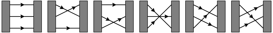
Figure 3.8: Schematic representation of the $3Q$ contribution to matrix elements. Each quark line stands for the color, flavor and spin contractions $\delta^{\alpha_{i}}_{\alpha^{\prime}_{i}}\delta^{f_{i}}_{f^{\prime}_{i}}\delta^{\sigma_{i}}_{\sigma^{\prime}_{i}}\int\mathrm{d}z^{\prime}_{i}\,\mathrm{d}^{2}\mathbf{p}^{\prime}_{i\perp}\delta(z_{i}-z^{\prime}_{i})\delta^{(2)}(\mathbf{p}_{i\perp}-\mathbf{p}^{\prime}_{i\perp})$ with the primed variables referring to $\Psi^{(3){\dagger}}(B)$ (right rectangle) and the unprimed ones to $\Psi^{(3)}(B)$ (left rectangle). A crossing of these quark lines corresponds to an anticommutation of two creation or annihilation operators and thus introduces a minus sign. This sign is however compensated by the one coming from the contraction of $\epsilon$ tensors with color indices. Since only valence quarks are involved all those diagrams are equivalent to the first one.

From eqs. (3.38) and (3.48) one can express the normalization of the $3Q$ component of baryon wave functions as

$$\mathcal{N}^{(3)}(B) = 36\,T(B)^{f_{1}f_{2}f_{3}}_{j_{1}j_{2}j_{3},k}T(B)_{f_{1}f_{2}f_{3}}^{l_{1}l_{2}l_{3},k}\int\mathrm{d}z_{1,2,3}\,\frac{\mathrm{d}^{2}\mathbf{p}_{1,2,3\perp}}{(2\pi)^{6}}\,\delta(z_{1}+z_{2}+z_{3}-1)(2\pi)^{2}\delta^{(2)}(\mathbf{p}_{1\perp}+\mathbf{p}_{2\perp}+\mathbf{p}_{3\perp})$$ (3.51)

$$\times F^{j_{1}\sigma_{1}}(p_{1})F^{j_{2}\sigma_{2}}(p_{2})F^{j_{3}\sigma_{3}}(p_{3})F^{\dagger}_{l_{1}\sigma_{1}}(p_{1})F^{\dagger}_{l_{2}\sigma_{2}}(p_{2})F^{\dagger}_{l_{3}\sigma_{3}}(p_{3})\qquad\textrm{no summation on $k$!}$$

where $F^{j\sigma}(p)\equiv F^{j\sigma}(z,\mathbf{p}_{\perp})$ is the discrete-level wave function (3.35)+(3.36).

All charges considered in this thesis are obtained by means of one-quark operators. These charges are computed by inserting the corresponding operator in each quark line. In the $3Q$ sector there is no antiquark which means that the $b^{\dagger}b$ part of the operator does not play. As in the $3Q$ normalization one gets the factor 36 from all contractions. Since valence quarks are equivalent the insertion of the operator in all three quark lines gives three times the same result. Let the third quark line be the one where the operator is inserted, see Fig. 3.9. If we denote by $\int(\mathrm{d}p_{1-3})$ the integrals over momenta with the $\delta$-functions as in eq. (3.51) one obtains the following expression for matrix element of the charge $Q$

$$Q^{(3)}(1\to 2) = 36\,T(1)^{f_{1}f_{2}f_{3}}_{j_{1}j_{2}j_{3},k}T(2)_{f_{1}f_{2}g_{3}}^{l_{1}l_{2}l_{3},l}\int(\mathrm{d}p_{1-3})$$ (3.52)

$$\times \Big{[}F^{j_{1}\sigma_{1}}(p_{1})F^{j_{2}\sigma_{2}}(p_{2})F^{j_{3}\sigma_{3}}(p_{3})\Big{]}\left[F^{\dagger}_{l_{1}\sigma_{1}}(p_{1})F^{\dagger}_{l_{2}\sigma_{2}}(p_{2})F^{\dagger}_{l_{3}\tau_{3}}(p_{3})\right]\left[3M^{\tau_{3}}_{\sigma_{3}}J^{g_{3}}_{f_{3}}\right].$$

where $J^{g_{3}}_{f_{3}}$ is the flavor content of the operator and $M^{\tau_{3}}_{\sigma_{3}}$ is the action of the operator on the quark spin. For example the vector operator is blind concerning the quark spin and thus $M^{\tau_{3}}_{\sigma_{3}}=\delta^{\tau_{3}}_{\sigma_{3}}$. The axial operator gives different signs to quarks with spin up and spin down and thus $M^{\tau_{3}}_{\sigma_{3}}=(\sigma_{3})^{\tau_{3}}_{\sigma_{3}}$. We consider here for simplicity only matrix elements in the limit of zero momentum transfer.

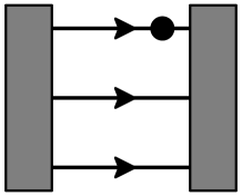
Figure 3.9: Schematic representation of the $3Q$ contribution to a charge. The black dot stands for the one-quark operator. Since all three quark lines are equivalent one has three times this specific contribution.

3.6.2 $5Q$ contributions

In the $5Q$ sector due to the presence of a quark-antiquark pair more diagrams are possible. Using the fact that valence quarks are equivalent only two types of diagrams survive: the direct and the exchange ones (see Fig. 3.10).

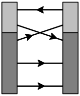
Figure 3.10: Schematic representation of the $5Q$ direct (left) and exchange (right) contributions to matrix elements.

In the former one contracts the $a^{\dagger}$ from the pair wave function with the $a$ in the conjugate pair and all the valence operators are contracted with each other. As in the $3Q$ case there are 6 equivalent possibilities but the contractions in color give now a factor of $6\cdot 3=\epsilon^{\alpha_{1}\alpha_{2}\alpha_{3}}\epsilon_{\alpha_{1}\alpha_{2}\alpha_{3}}\delta^{\alpha}_{\alpha}$ because of the sum over color in the pair, giving then a total factor of 108. In the exchange contribution one contracts the $a^{\dagger}$ from the pair with one of the three $a$’s from the conjugate discrete level. Vice versa, the $a$ from the conjugate pair is contracted with one of the three $a^{\dagger}$’s from the discrete level. There are at all 18 equivalent possibilities but the contractions in color give only a factor of $6=\epsilon^{\alpha_{1}\alpha_{2}\alpha}\epsilon_{\alpha_{1}\alpha_{2}\alpha_{3}}\delta^{\alpha_{3}}_{\alpha}$ and so one gets also a global factor of 108 for the exchange contribution but with an additional minus sign because one has to anticommute fermion operators to obtain exchange terms. We thus obtain the following expression for the $5Q$ normalization

$$\mathcal{N}^{(5)}(B) = 108\,T(B)^{f_{1}f_{2}f_{3}f_{4},j_{5}}_{j_{1}j_{2}j_{3}j_{4},f_{5},k}T(B)_{f_{1}f_{2}g_{3}g_{4},l_{5}}^{l_{1}l_{2}l_{3}l_{4},f_{5},k}\int(\mathrm{d}p_{1-5})$$ (3.53)

$$\times F^{j_{1}\sigma_{1}}(p_{1})F^{j_{2}\sigma_{2}}(p_{2})F^{j_{3}\sigma_{3}}(p_{3})W^{j_{4}\sigma_{4}}_{j_{5}\sigma_{5}}(p_{4},p_{5})F^{\dagger}_{l_{1}\sigma_{1}}(p_{1})F^{\dagger}_{l_{2}\sigma_{2}}(p_{2})$$

$$\times \left[F^{\dagger}_{l_{3}\sigma_{3}}(p_{3})W_{c\,l_{4}\sigma_{4}}^{l_{5}\sigma_{5}}(p_{4},p_{5})\delta^{g_{3}}_{f_{3}}\delta^{g_{4}}_{f_{4}}-F^{\dagger}_{l_{3}\sigma_{4}}(p_{4})W_{c\,l_{4}\sigma_{3}}^{l_{5}\sigma_{5}}(p_{3},p_{5})\delta^{g_{3}}_{f_{4}}\delta^{g_{4}}_{f_{3}}\right]$$

no summation on $$k$$!

where we have denoted

$$\int(\mathrm{d}p_{1-5})=\int\mathrm{d}z_{1-5}\,\delta(z_{1}+\ldots+z_{5}-1)\int\frac{\mathrm{d}^{2}\mathbf{p}_{1-5\perp}}{(2\pi)^{10}}\,(2\pi)^{2}\delta^{(2)}(\mathbf{p}_{1\perp}+\ldots+\mathbf{p}_{5\perp}).$$ (3.54)

Concerning the charges we have three types of direct contributions (antiquark, sea quark and valence quarks) and four types of exchange contributions (antiquark, exchange of the sea quark with a valence quark and other valence quarks).

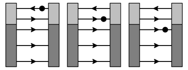
Figure 3.11: Schematic representation of the three types of $5Q$ direct contributions to the charges.

Figure 3.12: Schematic representation of the four types of $5Q$ exchange contributions to the charges.

From the schematic representations of these contributions (see Figs. 3.12 and 3.12) it is easy to write the transitions.

Direct diagram:

$$Q^{(5)\textrm{direct}}(1\to 2) = 108\,T(1)^{f_{1}f_{2}f_{3}f_{4},j_{5}}_{j_{1}j_{2}j_{3}j_{4},f_{5},k}T(2)_{f_{1}f_{2}g_{3}g_{4},l_{5}}^{l_{1}l_{2}l_{3}l_{4},g_{5},l}\int(\mathrm{d}p_{1-5})$$ (3.55)

$$\times F^{j_{1}\sigma_{1}}(p_{1})F^{j_{2}\sigma_{2}}(p_{2})F^{j_{3}\sigma_{3}}(p_{3})W^{j_{4}\sigma_{4}}_{j_{5}\sigma_{5}}(p_{4},p_{5})F^{\dagger}_{l_{1}\sigma_{1}}(p_{1})F^{\dagger}_{l_{2}\sigma_{2}}(p_{2})F^{\dagger}_{l_{3}\tau_{3}}(p_{3})W_{c\,l_{4}\tau_{4}}^{l_{5}\tau_{5}}(p_{4},p_{5})$$

$$\times \left[-\delta^{g_{3}}_{f_{3}}\delta^{g_{4}}_{f_{4}}J^{f_{5}}_{g_{5}}\delta^{\tau_{3}}_{\sigma_{3}}\delta^{\tau_{4}}_{\sigma_{4}}M_{\tau_{5}}^{\sigma_{5}}+\delta^{g_{3}}_{f_{3}}J^{g_{4}}_{f_{4}}\delta^{f_{5}}_{g_{5}}\delta^{\tau_{3}}_{\sigma_{3}}M^{\tau_{4}}_{\sigma_{4}}\delta_{\tau_{5}}^{\sigma_{5}}+3J^{g_{3}}_{f_{3}}\delta^{g_{4}}_{f_{4}}\delta^{f_{5}}_{g_{5}}M^{\tau_{3}}_{\sigma_{3}}\delta^{\tau_{4}}_{\sigma_{4}}\delta_{\tau_{5}}^{\sigma_{5}}\right].$$

Exchange diagram:

$$Q^{(5)\textrm{exchange}}(1\to 2) = -108\,T(1)^{f_{1}f_{2}f_{3}f_{4},j_{5}}_{j_{1}j_{2}j_{3}j_{4},f_{5},k}T(2)_{f_{1}g_{2}g_{3}g_{4},l_{5}}^{l_{1}l_{2}l_{3}l_{4},g_{5},l}\int(\mathrm{d}p_{1-5})$$ (3.56)

$$\times F^{j_{1}\sigma_{1}}(p_{1})F^{j_{2}\sigma_{2}}(p_{2})F^{j_{3}\sigma_{3}}(p_{3})W^{j_{4}\sigma_{4}}_{j_{5}\sigma_{5}}(p_{4},p_{5})F^{\dagger}_{l_{1}\sigma_{1}}(p_{1})F^{\dagger}_{l_{2}\tau_{2}}(p_{2})F^{\dagger}_{l_{3}\tau_{3}}(p_{3})W_{c\,l_{4}\tau_{4}}^{l_{5}\tau_{5}}(p_{3},p_{5})$$

$$\times \left[-\delta^{g_{2}}_{f_{2}}\delta^{g_{4}}_{f_{3}}\delta^{g_{3}}_{f_{4}}J^{f_{5}}_{g_{5}}\delta^{\tau_{2}}_{\sigma_{2}}\delta^{\tau_{4}}_{\sigma_{3}}\delta^{\tau_{3}}_{\sigma_{4}}M_{\tau_{5}}^{\sigma_{5}}+\delta^{g_{2}}_{f_{2}}\delta^{g_{4}}_{f_{3}}J^{g_{3}}_{f_{4}}\delta^{f_{5}}_{g_{5}}\delta^{\tau_{2}}_{\sigma_{2}}\delta^{\tau_{4}}_{\sigma_{3}}M^{\tau_{3}}_{\sigma_{4}}\delta_{\tau_{5}}^{\sigma_{5}}\right.$$

$$+\left.\delta^{g_{2}}_{f_{2}}J^{g_{4}}_{f_{3}}\delta^{g_{3}}_{f_{4}}\delta^{f_{5}}_{g_{5}}\delta^{\tau_{2}}_{\sigma_{2}}M^{\tau_{4}}_{\sigma_{3}}\delta^{\tau_{3}}_{\sigma_{4}}\delta_{\tau_{5}}^{\sigma_{5}}+2J^{g_{2}}_{f_{2}}\delta^{g_{4}}_{f_{3}}\delta^{g_{3}}_{f_{4}}\delta^{f_{5}}_{g_{5}}M^{\tau_{2}}_{\sigma_{2}}\delta^{\tau_{4}}_{\sigma_{3}}\delta^{\tau_{3}}_{\sigma_{4}}\delta_{\tau_{5}}^{\sigma_{5}}\right].$$

3.6.3 $7Q$ contributions

In the $7Q$ sector where two quark-antiquark pairs are involved the number of possible diagrams grows. These two pairs may remain unchanged (see Fig. 3.14) or exchange one of their constituents (see Fig. 3.14).

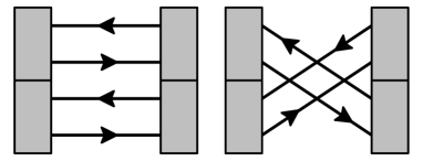
Figure 3.13: Contractions of two quark-antiquark pairs leaving them unchanged.

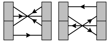
Figure 3.14: Contractions of two quark-antiquark pairs where one of the constituents is exchanged.

The pairs are in fact also equivalent and can be exchanged without any change in the result. This means that diagrams in Fig. 3.14 are equivalent, the same for those in Fig. 3.14. Finally after all contractions only five non-equivalent diagrams survive, see Fig. 3.15.

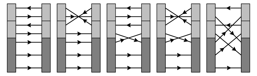
Figure 3.15: Schematic representation of the $7Q$ contributions to matrix elements.

The factor associated to each of these diagrams can easily be obtained since it is just a game of combinatorics. We give in Appendix B some general tools to find all these diagrams and their respective factor in any $nQ$ Fock sector. The $7Q$ factors are treated as explicit examples. With these tools one can obtain systematically all the contributions with the factor and the sign by means of diagrams only. One avoids thus the tedious work of contracting all creation-annihilation operators.

The $7Q$ normalization has the following form

$$\mathcal{N}^{(7)}(B) = 216\,T(B)^{f_{1}f_{2}f_{3}f_{4}f_{6},j_{5}j_{7}}_{j_{1}j_{2}j_{3}j_{4}j_{6},f_{5}f_{7},k}T(B)_{f_{1}g_{2}g_{3}g_{4}g_{6},l_{5}l_{7}}^{l_{1}l_{2}l_{3}l_{4}l_{6},g_{5}g_{7},k}\int(\mathrm{d}p_{1-7})$$ (3.57)

$$\times F^{j_{1}\sigma_{1}}(p_{1})F^{j_{2}\sigma_{2}}(p_{2})F^{j_{3}\sigma_{3}}(p_{3})W^{j_{4}\sigma_{4}}_{j_{5}\sigma_{5}}(p_{4},p_{5})W^{j_{6}\sigma_{6}}_{j_{7}\sigma_{7}}(p_{6},p_{7})F^{\dagger}_{l_{1}\sigma_{1}}(p_{1})$$

$$\times \Big{[}3F^{\dagger}_{l_{2}\sigma_{2}}(p_{2})F^{\dagger}_{l_{3}\sigma_{3}}(p_{3})W_{c\,l_{4}\sigma_{4}}^{l_{5}\sigma_{5}}(p_{4},p_{5})W_{c\,l_{6}\sigma_{6}}^{l_{7}\sigma_{7}}(p_{6},p_{7})\delta^{g_{2}}_{f_{2}}\delta^{g_{3}}_{f_{3}}\delta^{g_{4}}_{f_{4}}\delta^{f_{5}}_{g_{5}}\delta^{g_{6}}_{f_{6}}\delta^{f_{7}}_{g_{7}}$$

$$- F^{\dagger}_{l_{2}\sigma_{2}}(p_{2})F^{\dagger}_{l_{3}\sigma_{3}}(p_{3})W_{c\,l_{4}\sigma_{4}}^{l_{5}\sigma_{7}}(p_{4},p_{7})W_{c\,l_{6}\sigma_{6}}^{l_{7}\sigma_{5}}(p_{6},p_{5})\delta^{g_{2}}_{f_{2}}\delta^{g_{3}}_{f_{3}}\delta^{g_{4}}_{f_{4}}\delta^{f_{7}}_{g_{5}}\delta^{g_{6}}_{f_{6}}\delta^{f_{5}}_{g_{7}}$$

$$- 6F^{\dagger}_{l_{2}\sigma_{2}}(p_{2})F^{\dagger}_{l_{3}\sigma_{4}}(p_{4})W_{c\,l_{4}\sigma_{3}}^{l_{5}\sigma_{5}}(p_{3},p_{5})W_{c\,l_{6}\sigma_{6}}^{l_{7}\sigma_{7}}(p_{6},p_{7})\delta^{g_{2}}_{f_{2}}\delta^{g_{3}}_{f_{4}}\delta^{g_{4}}_{f_{3}}\delta^{f_{5}}_{g_{5}}\delta^{g_{6}}_{f_{6}}\delta^{f_{7}}_{g_{7}}$$

$$+ 2F^{\dagger}_{l_{2}\sigma_{2}}(p_{2})F^{\dagger}_{l_{3}\sigma_{4}}(p_{4})W_{c\,l_{4}\sigma_{3}}^{l_{5}\sigma_{7}}(p_{3},p_{7})W_{c\,l_{6}\sigma_{6}}^{l_{7}\sigma_{5}}(p_{6},p_{5})\delta^{g_{2}}_{f_{2}}\delta^{g_{3}}_{f_{4}}\delta^{g_{4}}_{f_{3}}\delta^{f_{7}}_{g_{5}}\delta^{g_{6}}_{f_{6}}\delta^{f_{5}}_{g_{7}}$$

$$+ 2F^{\dagger}_{l_{2}\sigma_{4}}(p_{4})F^{\dagger}_{l_{3}\sigma_{6}}(p_{6})W_{c\,l_{4}\sigma_{2}}^{l_{5}\sigma_{5}}(p_{2},p_{5})W_{c\,l_{6}\sigma_{3}}^{l_{7}\sigma_{7}}(p_{3},p_{7})\delta^{g_{2}}_{f_{4}}\delta^{g_{3}}_{f_{6}}\delta^{g_{4}}_{f_{2}}\delta^{f_{5}}_{g_{5}}\delta^{g_{6}}_{f_{3}}\delta^{f_{7}}_{g_{7}}\Big{]}$$

no summation on $$k$$!

Here is the explicit expression for the contribution to charges represented by the first diagram in Fig. 3.15

$$Q^{(7)\textrm{direct}}(1\to 2) = 648\,T(1)^{f_{1}f_{2}f_{3}f_{4}f_{6},j_{5}j_{7}}_{j_{1}j_{2}j_{3}j_{4}j_{6},f_{5}f_{7},k}T(2)_{f_{1}f_{2}g_{3}f_{4}g_{6},l_{5}l_{7}}^{l_{1}l_{2}l_{3}l_{4}l_{6},f_{5}g_{7},l}\int(\mathrm{d}p_{1-7})$$ (3.58)

$$\times F^{j_{1}\sigma_{1}}(p_{1})F^{j_{2}\sigma_{2}}(p_{2})F^{j_{3}\sigma_{3}}(p_{3})W^{j_{4}\sigma_{4}}_{j_{5}\sigma_{5}}(p_{4},p_{5})F^{\dagger}_{l_{1}\sigma_{1}}(p_{1})F^{\dagger}_{l_{2}\sigma_{2}}(p_{2})F^{\dagger}_{l_{3}\tau_{3}}(p_{3})W_{c\,l_{4}\tau_{4}}^{l_{5}\tau_{5}}(p_{4},p_{5})$$

$$\times \left[-2\delta^{g_{3}}_{f_{3}}\delta^{g_{6}}_{f_{6}}J^{f_{7}}_{g_{7}}\delta^{\tau_{3}}_{\sigma_{3}}\delta^{\tau_{6}}_{\sigma_{6}}M_{\tau_{7}}^{\sigma_{7}}+2\delta^{g_{3}}_{f_{3}}J^{g_{6}}_{f_{6}}\delta^{f_{7}}_{g_{7}}\delta^{\tau_{3}}_{\sigma_{3}}M^{\tau_{6}}_{\sigma_{6}}\delta_{\tau_{7}}^{\sigma_{7}o}+3J^{g_{3}}_{f_{3}}\delta^{g_{6}}_{f_{6}}\delta^{f_{7}}_{g_{7}}M^{\tau_{3}}_{\sigma_{3}}\delta^{\tau_{6}}_{\sigma_{6}}\delta_{\tau_{7}}^{\sigma_{7}}\right].$$

The factor 2 in front of the first and second terms reflects the fact that the action of the operator on both quark-antiquark pairs is the same. The contributions of the other diagrams can easily be obtained but have been neglected in the present thesis. We will discuss this point later.

3.7 Scalar overlap integrals

The computation of matrix elements has been done in two steps. The first step is the contraction over all flavor $(f,g)$, isospin $(j,l)$ and spin $(\sigma,\tau)$ indices. All charges are then reduced to linear combinations of a finite set of scalar integrals over longitudinal $z$ and transverse $\mathbf{p}_{\perp}$ momenta. These integrals are just overlaps of valence and pair wave functions. The integrals over relative transverse momenta in the quark-antiquark pair are generally UV divergent. This divergence should be cut by the momentum-dependent dynamical quark mass $M(p)$, see eq. (3.1). Following the authors of [118] we mimic the fall-off of $M(p)$ by the Pauli-Villars cutoff at $M_{\textrm{PV}}=556.8$ MeV (this value being chosen from the requirement that the pion decay constant $F_{\pi}=93$ MeV is reproduced from $M(0)=345$ MeV).

The complexity of these integrals is directly related to the complexity of the diagram. The simplest ones are the “direct” diagrams where no exchange of quarks is involved. In this case valence quarks and sea pairs keep their identity. This is reflected by the fact that the integrals can be performed in many steps and that valence and sea pairs variables almost decouple.

3.7.1 $3Q$ scalar integrals

For convenience we introduce the probability distribution $\Phi^{I}(z,\mathbf{q}_{\perp})$ that three valence quarks leave longitudinal fraction $z=q_{z}/\mathcal{M}$ and transverse momentum $\mathbf{q}_{\perp}$ to the quark-antiquark pair(s) with $I=V,A,T,M$ referring to the vector, axial, tensor or magnetic case

$$\Phi^{I}(z,\mathbf{q}_{\perp})=\int\mathrm{d}z_{1,2,3}\frac{\mathrm{d}^{2}\mathbf{p}_{1,2,3\perp}}{(2\pi)^{6}}\,\delta(z+z_{1}+z_{2}+z_{3}-1)(2\pi)^{2}\delta^{(2)}(\mathbf{q}_{\perp}+\mathbf{p}_{1\perp}+\mathbf{p}_{2\perp}+\mathbf{p}_{3\perp})D^{I}(p_{1},p_{2},p_{3}).$$ (3.59)

The function $D^{I}(p_{1},p_{2},p_{3})$ is given in terms of the upper and lower valence wave functions $h(p)$ and $j(p)$ and is constructed from the product of all valence wave functions $F$ and the current operator. Its explicit form in the vector, axial, tensor or magnetic case can be found in the corresponding chapters.

In the $3Q$ sector there is no quark-antiquark pair. This means that the whole baryon momentum is carried by the valence quarks. The $3Q$ scalar integrals are thus simply $\Phi^{I}(0,0)$.

3.7.2 $5Q$ direct scalar integrals

In the $5Q$ sector there is one quark-antiquark pair. Thanks to the simplicity of the direct diagram the corresponding scalar overlap integrals can be written in two parts: purely valence $\Phi^{I}$ and sea $G_{J}$

$$K^{I}_{J}=\frac{M^{2}}{2\pi}\int\frac{\mathrm{d}^{3}\mathbf{q}}{(2\pi)^{3}}\,\Phi^{I}\left(\frac{q_{z}}{\mathcal{M}},\mathbf{q}_{\perp}\right)\theta(q_{z})\,q_{z}\,G_{J}(q_{z},\mathbf{q}_{\perp})$$ (3.60)

where $G_{J}$ is a quark-antiquark probability distribution and $J=\pi\pi,33,332,\sigma\sigma,3\sigma$. These distributions are obtained by contracting two quark-antiquark wave functions $W$, see eq. (3.31) and regularized by means of Pauli-Villars procedure

$$G_{\pi\pi}(q_{z},\mathbf{q}_{\perp}) = \Pi^{2}(\mathbf{q})\int^{1}_{0}\mathrm{d}y\int\frac{\mathrm{d}^{2}\mathcal{Q}_{\perp}}{(2\pi)^{2}}\frac{\mathcal{Q}^{2}_{\perp}+M^{2}}{(\mathcal{Q}^{2}_{\perp}+M^{2}+y(1-y)\mathbf{q}^{2})^{2}}-(M\to M_{\textrm{PV}}),$$ (3.61)

$$G_{33}(q_{z},\mathbf{q}_{\perp}) = \frac{q_{z}^{2}}{\mathbf{q}^{2}}\,G_{\pi\pi}(q_{z},\mathbf{q}_{\perp}),$$ (3.62)

$$G_{332}(q_{z},\mathbf{q}_{\perp}) = \frac{q_{z}}{\mathbf{q}^{2}}\,G_{\pi\pi}(q_{z},\mathbf{q}_{\perp}),$$ (3.63)

$$G_{\sigma\sigma}(q_{z},\mathbf{q}_{\perp}) = \Sigma^{2}(\mathbf{q})\int^{1}_{0}\mathrm{d}y\int\frac{\mathrm{d}^{2}\mathcal{Q}_{\perp}}{(2\pi)^{2}}\frac{\mathcal{Q}^{2}_{\perp}+M^{2}(2y-1)^{2}}{(\mathcal{Q}^{2}_{\perp}+M^{2}+y(1-y)\mathbf{q}^{2})^{2}}-(M\to M_{\textrm{PV}}),$$ (3.64)

$$G_{3\sigma}(q_{z},\mathbf{q}_{\perp}) = \frac{q_{z}}{|\mathbf{q}|}\,\Pi(\mathbf{q})\Sigma(\mathbf{q})\int^{1}_{0}\mathrm{d}y\int\frac{\mathrm{d}^{2}\mathcal{Q}_{\perp}}{(2\pi)^{2}}\frac{\mathcal{Q}^{2}_{\perp}+M^{2}(2y-1)}{(\mathcal{Q}^{2}_{\perp}+M^{2}+y(1-y)\mathbf{q}^{2})^{2}}-(M\to M_{\textrm{PV}})$$ (3.65)

where $q_{z}=z\mathcal{M}=(z_{4}+z_{5})\mathcal{M}$ and $\mathbf{q}_{\perp}=\mathbf{p}_{4\perp}+\mathbf{p}_{5\perp}$. In summary, the upper index $I$ refers to the valence part and the lower index $J$ to the sea part. Axial integrals may thus have the vector index $V$ since it refers only the valence structure. Index $J$ refers to the transition experienced by the quark-antiquark pair.

Index $J$	Transition
$\pi\pi,\pi 3,33$	pseudoscalar$\leftrightarrow$	pseudoscalar
$\sigma\sigma$	scalar$\leftrightarrow$	scalar
$\pi\sigma,3\sigma$	pseudoscalar$\leftrightarrow$	scalar

3.7.3 $5Q$ exchange scalar integrals

The exchange diagram mixes valence and non-valence quarks. Therefore the integrals cannot be decomposed into a purely valence part and a sea part. However since valence quarks are equivalent a decomposition is still possible. One part is the distribution of two valence quarks $\phi$ and the other part is the rest, i.e. the third valence quark entangled with the pair. This diagram has been studied in the non-relativistic limit $j=0$ to keep things as simple as possible. The integrals have then the following structure

$$K_{J}=\frac{M^{2}}{2\pi}\int(\mathrm{d}p_{3,4,5})\,\phi\left(\mathcal{Z},\mathbf{P}_{\perp}\right)\frac{\mathcal{M}^{2}}{2\pi Z^{\prime}Z}\,I_{J}(z_{3,4,5},\mathbf{p}_{3,4,5\perp})h(p_{3})h(p_{4}),$$ (3.66)

where $\mathcal{Z}=z_{3}+z_{4}+z_{5}$, $\mathbf{P}_{\perp}=(\mathbf{p}_{3}+\mathbf{p}_{4}+\mathbf{p}_{5})_{\perp}$, $Z$ is given by eq. (3.28) with $z=z_{4}$, $\mathbf{p}_{\perp}=\mathbf{p}_{4\perp}$ and $z^{\prime}=z_{5}$, $\mathbf{p}^{\prime}_{\perp}=\mathbf{p}_{5\perp}$ while $Z^{\prime}$ is the same but with the replacement $4\to 3$. The function $I_{J}(z_{3,4,5},\mathbf{p}_{3,4,5\perp})$ stands for the thirteen integrands

$$I_{1} = \Sigma(\mathbf{q}^{\prime})\Sigma(\mathbf{q})\left(\mathbf{Q}^{\prime}_{\perp}\cdot\mathbf{Q}_{\perp}+M^{2}(z_{5}-z_{3})(z_{5}-z_{4})\right),$$ (3.67)

$$I_{2} = \Pi(\mathbf{q}^{\prime})\Pi(\mathbf{q})\,\frac{q^{\prime}\cdot q}{|\mathbf{q}^{\prime}||\mathbf{q}|}\left(\mathbf{Q}^{\prime}_{\perp}\cdot\mathbf{Q}_{\perp}+M^{2}(z_{5}+z_{3})(z_{5}+z_{4})\right),$$ (3.68)

$$I_{3} = \Pi(\mathbf{q}^{\prime})\Pi(\mathbf{q})\,\frac{\mathbf{q}^{\prime}_{\perp}\times\mathbf{q}_{\perp}}{|\mathbf{q}^{\prime}||\mathbf{q}|}\,(\mathbf{Q}^{\prime}_{\perp}\times\mathbf{Q}_{\perp}),$$ (3.69)

$$I_{4} = \Pi(\mathbf{q}^{\prime})\Pi(\mathbf{q})\,\frac{M(\mathbf{q}^{\prime}_{\perp}q_{z}-\mathbf{q}_{\perp}q^{\prime}_{z})}{|\mathbf{q}^{\prime}||\mathbf{q}|}\cdot\left(\mathbf{Q}_{\perp}-\mathbf{Q}^{\prime}_{\perp}\right),$$ (3.70)

$$I_{5} = \Pi(\mathbf{q}^{\prime})\Pi(\mathbf{q})\,\frac{q^{\prime}_{z}q_{z}}{|\mathbf{q}^{\prime}||\mathbf{q}|}\left(\mathbf{Q}^{\prime}_{\perp}\cdot\mathbf{Q}_{\perp}+M^{2}(z_{5}+z_{3})(z_{5}+z_{4})\right),$$ (3.71)

$$I_{6} = \Sigma(\mathbf{q}^{\prime})\Pi(\mathbf{q})\,\frac{q_{z}}{|\mathbf{q}|}\left(\mathbf{Q}^{\prime}_{\perp}\cdot\mathbf{Q}_{\perp}+M^{2}(z_{5}-z_{3})(z_{5}+z_{4})\right),$$ (3.72)

$$I_{7} = \Sigma(\mathbf{q}^{\prime})\Pi(\mathbf{q})\,\frac{M\mathbf{q}_{\perp}}{|\mathbf{q}|}\cdot\left(\mathbf{Q}^{\prime}_{\perp}(z_{5}+z_{4})-\mathbf{Q}_{\perp}(z_{5}-z_{3})\right),$$ (3.73)

$$I_{8} = \Sigma(\mathbf{q}^{\prime})\Sigma(\mathbf{q})\left(\mathbf{Q}^{\prime}_{\perp}\cdot\mathbf{Q}_{\perp}-M^{2}(z_{5}-z_{3})(z_{5}-z_{4})\right),$$ (3.74)

$$I_{9} = \Pi(\mathbf{q}^{\prime})\Pi(\mathbf{q})\,\frac{q^{\prime}\cdot q}{|\mathbf{q}^{\prime}||\mathbf{q}|}\left(\mathbf{Q}^{\prime}_{\perp}\cdot\mathbf{Q}_{\perp}-M^{2}(z_{5}+z_{3})(z_{5}+z_{4})\right),$$ (3.75)

$$I_{10} = \Pi(\mathbf{q}^{\prime})\Pi(\mathbf{q})\,\frac{M(\mathbf{q}^{\prime}_{\perp}q_{z}+\mathbf{q}_{\perp}q^{\prime}_{z})}{|\mathbf{q}^{\prime}||\mathbf{q}|}\cdot\left(\mathbf{Q}_{\perp}+\mathbf{Q}^{\prime}_{\perp}\right),$$ (3.76)

$$I_{11} = \Pi(\mathbf{q}^{\prime})\Pi(\mathbf{q})\,\frac{q^{\prime}_{z}q_{z}}{|\mathbf{q}^{\prime}||\mathbf{q}|}\left(\mathbf{Q}^{\prime}_{\perp}\cdot\mathbf{Q}_{\perp}-M^{2}(z_{5}+z_{3})(z_{5}+z_{4})\right),$$ (3.77)

$$I_{12} = \Sigma(\mathbf{q}^{\prime})\Pi(\mathbf{q})\,\frac{q_{z}}{|\mathbf{q}|}\left(\mathbf{Q}^{\prime}_{\perp}\cdot\mathbf{Q}_{\perp}-M^{2}(z_{5}-z_{3})(z_{5}+z_{4})\right),$$ (3.78)

$$I_{13} = \Sigma(\mathbf{q}^{\prime})\Pi(\mathbf{q})\,\frac{M\mathbf{q}_{\perp}}{|\mathbf{q}|}\cdot\left(\mathbf{Q}^{\prime}_{\perp}(z_{5}+z_{4})+\mathbf{Q}_{\perp}(z_{5}-z_{3})\right)$$ (3.79)

where $\mathbf{q}=((\mathbf{p}_{4}+\mathbf{p}_{5})_{\perp},(z_{4}+z_{5})\mathcal{M})$ and $\mathbf{Q}_{\perp}=z_{4}\mathbf{p}_{5\perp}-z_{5}\mathbf{p}_{4\perp}$. The primed variables stand for the same as the unprimed ones but with the replacement $4\to 3$. The regularization of those integrals is done exactly in the same way as for the direct contributions.

The function $\phi(\mathcal{Z},\mathbf{P}_{\perp})$ stands for the probability that two valence quarks “leave” the longitudinal fraction $\mathcal{Z}=z_{3}+z_{4}+z_{5}$ and the transverse momentum $\mathbf{P}_{\perp}=\mathbf{p}_{3\perp}+\mathbf{p}_{4\perp}+\mathbf{p}_{5\perp}$ to the rest of the partons. In the non-relativistic limit we have

$$\phi(\mathcal{Z},\mathbf{P}_{\perp})=\int\mathrm{d}z_{1,2}\frac{\mathrm{d}^{2}\mathbf{p}_{1,2\perp}}{(2\pi)^{4}}\,\delta(\mathcal{Z}+z_{1}+z_{2}-1)(2\pi)^{2}\delta^{(2)}(\mathbf{P}_{\perp}+\mathbf{p}_{1\perp}+\mathbf{p}_{2\perp})h^{2}(p_{1})h^{2}(p_{2}).$$ (3.80)

We have kept of course the same non-relativistic normalization of the discrete-level wave function $h(p)$ as in the direct contributions, i.e. such that $\Phi_{NR}(0,0)=\int(\mathrm{d}p)\,\phi(z,\mathbf{p}_{\perp})h^{2}(p)=1$.

3.7.4 $7Q$ scalar integrals

In the $7Q$ sector there are two quark-antiquark pairs. Thanks to the simplicity of the direct diagram the corresponding scalar overlap integrals can be written in two parts: purely valence $\Phi^{I}$ and sea $G_{J}$

$$K^{I}_{J}=\frac{M^{4}}{(2\pi)^{2}}\int\frac{\mathrm{d}^{3}\mathbf{q}}{(2\pi)^{3}}\frac{\mathrm{d}^{3}\mathbf{q}^{\prime}}{(2\pi)^{3}}\,\Phi^{I}\left(\frac{(q_{z}+q^{\prime}_{z})}{\mathcal{M}},\mathbf{q}_{\perp}+\mathbf{q}^{\prime}_{\perp}\right)\theta(q_{z})\,\theta(q^{\prime}_{z})\,q_{z}\,q^{\prime}_{z}\,G_{J}(q_{z},q^{\prime}_{z},\mathbf{q}_{\perp},\mathbf{q}^{\prime}_{\perp}).$$ (3.81)

where $J=\pi\pi\pi\pi,\pi\pi\pi\pi 2,\pi\pi 33,3333,\pi 3\pi 3,\sigma\sigma\pi\pi,\sigma\sigma 33,\sigma\sigma\sigma\sigma,\pi\pi 3\sigma,333\sigma,\pi 3\pi\sigma,\sigma\sigma 3\sigma$. These distributions are obtained by contracting four quark-antiquark wave functions $W$, see eq. (3.31) and regularized by means of Pauli-Villars procedure. They can in fact be expressed in terms of $G_{J}(q_{z},\mathbf{q}_{\perp})$ since in direct diagrams $Q\bar{Q}$ pairs keep their identity. Here are then the distributions in the $7Q$ sector

$$G_{\pi\pi\pi\pi}(q_{z},q^{\prime}_{z},\mathbf{q}_{\perp},\mathbf{q}^{\prime}_{\perp}) = G_{\pi\pi}(q_{z},\mathbf{q}_{\perp})\,G_{\pi\pi}(q^{\prime}_{z},\mathbf{q}^{\prime}_{\perp}),$$ (3.82)

$$G_{\pi\pi\pi\pi 2}(q_{z},q^{\prime}_{z},\mathbf{q}_{\perp},\mathbf{q}^{\prime}_{\perp}) = \frac{(\mathbf{q}\cdot\mathbf{q}^{\prime})^{2}}{\mathbf{q}^{2}\mathbf{q}^{\prime 2}}\,G_{\pi\pi}(q_{z},\mathbf{q}_{\perp})\,G_{\pi\pi}(q^{\prime}_{z},\mathbf{q}^{\prime}_{\perp}),$$ (3.83)

$$G_{\pi\pi 33}(q_{z},q^{\prime}_{z},\mathbf{q}_{\perp},\mathbf{q}^{\prime}_{\perp}) = G_{\pi\pi}(q_{z},\mathbf{q}_{\perp})\,G_{33}(q^{\prime}_{z},\mathbf{q}^{\prime}_{\perp}),$$ (3.84)

$$G_{3333}(q_{z},q^{\prime}_{z},\mathbf{q}_{\perp},\mathbf{q}^{\prime}_{\perp}) = G_{33}(q_{z},\mathbf{q}_{\perp})\,G_{33}(q^{\prime}_{z},\mathbf{q}^{\prime}_{\perp}),$$ (3.85)

$$G_{\pi 3\pi 3}(q_{z},q^{\prime}_{z},\mathbf{q}_{\perp},\mathbf{q}^{\prime}_{\perp}) = \frac{q_{z}q^{\prime}_{z}(\mathbf{q}\cdot\mathbf{q}^{\prime})}{\mathbf{q}^{2}\mathbf{q}^{\prime 2}}\,G_{\pi\pi}(q_{z},\mathbf{q}_{\perp})\,G_{\pi\pi}(q^{\prime}_{z},\mathbf{q}^{\prime}_{\perp}),$$ (3.86)

$$G_{\sigma\sigma\pi\pi}(q_{z},q^{\prime}_{z},\mathbf{q}_{\perp},\mathbf{q}^{\prime}_{\perp}) = G_{\sigma\sigma}(q_{z},\mathbf{q}_{\perp})\,G_{\pi\pi}(q^{\prime}_{z},\mathbf{q}^{\prime}_{\perp}),$$ (3.87)

$$G_{\sigma\sigma 33}(q_{z},q^{\prime}_{z},\mathbf{q}_{\perp},\mathbf{q}^{\prime}_{\perp}) = G_{\sigma\sigma}(q_{z},\mathbf{q}_{\perp})\,G_{33}(q^{\prime}_{z},\mathbf{q}^{\prime}_{\perp}),$$ (3.88)

$$G_{\sigma\sigma\sigma\sigma}(q_{z},q^{\prime}_{z},\mathbf{q}_{\perp},\mathbf{q}^{\prime}_{\perp}) = G_{\sigma\sigma}(q_{z},\mathbf{q}_{\perp})\,G_{\sigma\sigma}(q^{\prime}_{z},\mathbf{q}^{\prime}_{\perp}),$$ (3.89)

$$G_{\pi\pi 3\sigma}(q_{z},q^{\prime}_{z},\mathbf{q}_{\perp},\mathbf{q}^{\prime}_{\perp}) = G_{\pi\pi}(q_{z},\mathbf{q}_{\perp})\,G_{3\sigma}(q^{\prime}_{z},\mathbf{q}^{\prime}_{\perp}),$$ (3.90)

$$G_{333\sigma}(q_{z},q^{\prime}_{z},\mathbf{q}_{\perp},\mathbf{q}^{\prime}_{\perp}) = G_{33}(q_{z},\mathbf{q}_{\perp})\,G_{3\sigma}(q^{\prime}_{z},\mathbf{q}^{\prime}_{\perp}),$$ (3.91)

$$G_{\pi 3\pi\sigma}(q_{z},q^{\prime}_{z},\mathbf{q}_{\perp},\mathbf{q}^{\prime}_{\perp}) = \frac{q_{z}(\mathbf{q}\cdot\mathbf{q}^{\prime})}{q^{\prime}_{z}\mathbf{q}^{2}}\,G_{\pi\pi}(q_{z},\mathbf{q}_{\perp})\,G_{3\sigma}(q^{\prime}_{z},\mathbf{q}^{\prime}_{\perp}),$$ (3.92)

$$G_{\sigma\sigma 3\sigma}(q_{z},q^{\prime}_{z},\mathbf{q}_{\perp},\mathbf{q}^{\prime}_{\perp}) = G_{\sigma\sigma}(q_{z},\mathbf{q}_{\perp})\,G_{3\sigma}(q^{\prime}_{z},\mathbf{q}^{\prime}_{\perp})$$ (3.93)

where $q_{z}=z\mathcal{M}=(z_{4}+z_{5})\mathcal{M}$, $q^{\prime}_{z}=z\mathcal{M}=(z_{6}+z_{7})\mathcal{M}$, $\mathbf{q}_{\perp}=\mathbf{p}_{4\perp}+\mathbf{p}_{5\perp}$ and $\mathbf{q}^{\prime}_{\perp}=\mathbf{p}_{6\perp}+\mathbf{p}_{7\perp}$.

Scalar integrals arising from the four exchange diagrams in the $7Q$ sector have not been computed. As we will show later, exchange diagrams give only negligible contributions and can therefore be ignored. Naively one could indeed expect exchange contributions to be smaller than direct ones. Direct diagrams correspond to the simple case where nothing really happens, all partons keep their role. On the contrary exchange diagrams describe modifications in the roles played by the partons and implies thus some correlations among quarks.

Chapter 4 Symmetry relations and parametrization

In this work we have studied baryons properties in flavor $SU(3)$ symmetry. Even though this symmetry is broken in nature, it gives quite a good estimation. With such an assumption all particles in a given representation are on the same footing and are related through pure flavor $SU(3)$ transformations. In other words, we need to concentrate only on, say, proton properties. Properties of the other octet members can be obtained from the proton one.

The naive non-relativistic quark model is based on a larger group $SU(6)$ that imbeds $SU(3)_{F}\times SU(2)_{S}$. In this approach, octet and decuplet baryons belong to the same supermultiplet. This yields relations between different $SU(3)$ multiplets and new ones within multiplets.

As one can see symmetry is very useful and convenient. In the next sections we give the explicit relations among baryons properties.

4.1 General flavor $SU(3)$ symmetry relations

Let us consider a charge $Q$, e.g. the vector, axial or tensor charge or even the electric charge and magnetic form factor. If the contribution of each flavor is known for a member in a given multiplet, then flavor $SU(3)$ symmetry allows one to find those contributions for all other members of the same multiplet. One could then use these flavor contributions as parameters for the given multiplet. We chose however to use another parametrization in order to emphasize some properties. The number of parameters depends on the multiplet under consideration.

Table 4.1: $SU(3)$ octet relations.

$B$	$Q^{(B)u}$	$Q^{(B)d}$	$Q^{(B)s}$
$p_{\mathbf{8}}^{+}$	$\alpha+\gamma$	$\beta+\gamma$	$\gamma$
$n_{\mathbf{8}}^{0}$	$\beta+\gamma$	$\alpha+\gamma$	$\gamma$
$\Lambda_{\mathbf{8}}^{0}$	$\frac{1}{6}(\alpha+4\beta)+\gamma$	$\frac{1}{6}(\alpha+4\beta)+\gamma$	$\frac{1}{3}(2\alpha-\beta)+\gamma$
$\Sigma_{\mathbf{8}}^{+}$	$\alpha+\gamma$	$\gamma$	$\beta+\gamma$
$\Sigma_{\mathbf{8}}^{0}$	$\frac{1}{2}\alpha+\gamma$	$\frac{1}{2}\alpha+\gamma$	$\beta+\gamma$
$\Sigma_{\mathbf{8}}^{-}$	$\gamma$	$\alpha+\gamma$	$\beta+\gamma$
$\Xi_{\mathbf{8}}^{0}$	$\beta+\gamma$	$\gamma$	$\alpha+\gamma$
$\Xi_{\mathbf{8}}^{-}$	$\gamma$	$\beta+\gamma$	$\alpha+\gamma$

For baryon octet one needs to use three parameters, e.g. $\alpha$, $\beta$ and $\gamma$ while for baryon decuplet and antidecuplet only two are needed, e.g. $\alpha^{\prime}$, $\beta^{\prime}$ and $\alpha^{\prime\prime}$, $\beta^{\prime\prime}$. Tables 4.1, 4.3 and 4.3 give for each flavor the parametrization of the contribution to the baryon charges.

Table 4.2: $SU(3)$ decuplet relations.

$B$	$Q^{(B)u}$	$Q^{(B)d}$	$Q^{(B)s}$
$\Delta_{\mathbf{10}}^{++}$	$3\alpha^{\prime}+\beta^{\prime}$	$\beta^{\prime}$	$\beta^{\prime}$
$\Delta_{\mathbf{10}}^{+}$	$2\alpha^{\prime}+\beta^{\prime}$	$\alpha^{\prime}+\beta^{\prime}$	$\beta^{\prime}$
$\Delta_{\mathbf{10}}^{0}$	$\alpha^{\prime}+\beta^{\prime}$	$2\alpha^{\prime}+\beta^{\prime}$	$\beta^{\prime}$
$\Delta_{\mathbf{10}}^{-}$	$\beta^{\prime}$	$3\alpha^{\prime}+\beta^{\prime}$	$\beta^{\prime}$
$\Sigma_{\mathbf{10}}^{+}$	$2\alpha^{\prime}+\beta^{\prime}$	$\beta^{\prime}$	$\alpha^{\prime}+\beta^{\prime}$
$\Sigma_{\mathbf{10}}^{0}$	$\alpha^{\prime}+\beta^{\prime}$	$\alpha^{\prime}+\beta^{\prime}$	$\alpha^{\prime}+\beta^{\prime}$
$\Sigma_{\mathbf{10}}^{-}$	$\beta^{\prime}$	$2\alpha^{\prime}+\beta^{\prime}$	$\alpha^{\prime}+\beta^{\prime}$
$\Xi_{\mathbf{10}}^{0}$	$\alpha^{\prime}+\beta^{\prime}$	$\beta^{\prime}$	$2\alpha^{\prime}+\beta^{\prime}$
$\Xi_{\mathbf{10}}^{-}$	$\beta^{\prime}$	$\alpha^{\prime}+\beta^{\prime}$	$2\alpha^{\prime}+\beta^{\prime}$
$\Omega_{\mathbf{10}}^{-}$	$\beta^{\prime}$	$\beta^{\prime}$	$3\alpha^{\prime}+\beta^{\prime}$

Table 4.3: $SU(3)$ antidecuplet relations.

$B$	$Q^{(B)u}$	$Q^{(B)d}$	$Q^{(B)s}$
$\Theta_{\mathbf{\overline{10}}}^{+}$	$2\alpha^{\prime\prime}+\beta^{\prime\prime}$	$2\alpha^{\prime\prime}+\beta^{\prime\prime}$	$-\alpha^{\prime\prime}+\beta^{\prime\prime}$
$p_{\mathbf{\overline{10}}}^{+}$	$2\alpha^{\prime\prime}+\beta^{\prime\prime}$	$\alpha^{\prime\prime}+\beta^{\prime\prime}$	$\beta^{\prime\prime}$
$n_{\mathbf{\overline{10}}}^{0}$	$\alpha^{\prime\prime}+\beta^{\prime\prime}$	$2\alpha^{\prime\prime}+\beta^{\prime\prime}$	$\beta^{\prime\prime}$
$\Sigma_{\mathbf{\overline{10}}}^{+}$	$2\alpha^{\prime\prime}+\beta^{\prime\prime}$	$\beta^{\prime\prime}$	$\alpha^{\prime\prime}+\beta^{\prime\prime}$
$\Sigma_{\mathbf{\overline{10}}}^{0}$	$\alpha^{\prime\prime}+\beta^{\prime\prime}$	$\alpha^{\prime\prime}+\beta^{\prime\prime}$	$\alpha^{\prime\prime}+\beta^{\prime\prime}$
$\Sigma_{\mathbf{\overline{10}}}^{-}$	$\beta^{\prime\prime}$	$2\alpha^{\prime\prime}+\beta^{\prime\prime}$	$\alpha^{\prime\prime}+\beta^{\prime\prime}$
$\Xi_{\mathbf{\overline{10}}}^{+}$	$2\alpha^{\prime\prime}+\beta^{\prime\prime}$	$-\alpha^{\prime\prime}+\beta^{\prime\prime}$	$2\alpha^{\prime\prime}+\beta^{\prime\prime}$
$\Xi_{\mathbf{\overline{10}}}^{0}$	$\alpha^{\prime\prime}+\beta^{\prime\prime}$	$\beta^{\prime\prime}$	$2\alpha^{\prime\prime}+\beta^{\prime\prime}$
$\Xi_{\mathbf{\overline{10}}}^{-}$	$\beta^{\prime\prime}$	$\alpha^{\prime\prime}+\beta^{\prime\prime}$	$2\alpha^{\prime\prime}+\beta^{\prime\prime}$
$\Xi_{\mathbf{\overline{10}}}^{--}$	$-\alpha^{\prime\prime}+\beta^{\prime\prime}$	$2\alpha^{\prime\prime}+\beta^{\prime\prime}$	$2\alpha^{\prime\prime}+\beta^{\prime\prime}$

Table 4.4: $SU(3)$ octet vector and axial transition relations.

Transitions		$g_{V,A}$	Transitions		$g_{V,A}$
$n_{\mathbf{8}}^{0}$$\to$	$p_{\mathbf{8}}^{+}$	$\alpha-\beta$	$\textrm{ }\Sigma_{\mathbf{8}}^{-}$$\to$	$n_{\mathbf{8}}^{0}$	$-\beta$
$\Sigma_{\mathbf{8}}^{-}$$\to$	$\Sigma_{\mathbf{8}}^{0}$	$\alpha/\sqrt{2}$	$\Xi_{\mathbf{8}}^{-}$$\to$	$\Sigma_{\mathbf{8}}^{0}$	$(\beta-\alpha)/\sqrt{2}$
$\Sigma_{\mathbf{8}}^{-}$$\to$	$\Lambda_{\mathbf{8}}^{0}$	$(\alpha-2\beta)/\sqrt{6}$	$\Xi_{\mathbf{8}}^{-}$$\to$	$\Lambda_{\mathbf{8}}^{0}$	$-(\alpha+\beta)/\sqrt{6}$
$\Sigma_{\mathbf{8}}^{0}$$\to$	$\Sigma_{\mathbf{8}}^{+}$	$-\alpha/\sqrt{2}$	$\Sigma_{\mathbf{8}}^{0}$$\to$	$p_{\mathbf{8}}^{+}$	$-\beta/\sqrt{2}$
$\Lambda_{\mathbf{8}}^{0}$$\to$	$\Sigma_{\mathbf{8}}^{+}$	$(\alpha-2\beta)/\sqrt{6}$	$\Lambda_{\mathbf{8}}^{0}$$\to$	$p_{\mathbf{8}}^{+}$	$(\beta-2\alpha)/\sqrt{6}$
$\Xi_{\mathbf{8}}^{-}$$\to$	$\Xi_{\mathbf{8}}^{0}$	$\beta$	$\Xi_{\mathbf{8}}^{0}$$\to$	$\Sigma_{\mathbf{8}}^{+}$	$\alpha-\beta$

This specific parametrization shows explicitly that one cannot access to all electric and magnetic parameters from total electric charges and magnetic moments alone or to all axial content from the isovector or octet charges alone. It is also clear that the singlet vector, axial and tensor charges are the same within a multiplet.

Some parameters can be interpreted if one considers the $3Q$ sector only. It implies that $\gamma,\beta^{\prime},\beta^{\prime\prime}=0$ and thus $\alpha,\beta$ are the contribution of (valence) $u,d$ quarks in the proton and $\alpha^{\prime}$ is the contribution of (valence) $u$ quarks in the $\Delta^{++}$. From the structure in Tables 4.1, 4.3 and 4.3 one could naively think that $\gamma,\beta^{\prime},\beta^{\prime\prime}$ represent the contribution of the $SU(3)$ symmetric sea. In fact these relations hold separately for valence quarks, sea quarks and antiquarks.

A few octet baryon decay constants are known from experiment. It is then interesting to express them in terms of our parameters $\alpha$ and $\beta$ ($\gamma$ disappears), see Table 4.4. In the literature they are usually expressed in terms of the Cabibbo parameters $F\&D$ [131]. Here is the link between both parametrization

$$\alpha=2F,\qquad\beta=F-D.$$ (4.1)

4.2 Flavor $SU(3)$ symmetry and magnetic moments

Let us discuss a little bit further flavor $SU(3)$ symmetry in relation with magnetic moments and transition magnetic moments. We have seen that magnetic form factors within a multiplet are related by the flavor symmetry and so are the magnetic moments. The total magnetic moments are obtained by the formula

$$\mu_{B}=e_{u}\,G_{M}^{(B)u}+e_{d}\,G_{M}^{(B)d}+e_{s}\,G_{M}^{(B)s}$$ (4.2)

where $e_{u}$, $e_{d}$ and $e_{s}$ are quark electric charges, i.e. 2/3, -1/3 and -1/3 respectively. If one considers magnetic transitions between multiplets, flavor symmetry will also impose relations and will even forbid some transitions. The $SU(3)$ prediction for magnetic moments and transition magnetic moments is greatly simplified by the use of the concept of $U$-spin. Let us briefly recall this concept.

4.2.1 Charge and $U$-spin

Flavor $SU(3)$ multiplets are usually represented in the $(I_{3},Y)$-basis, i.e. to each member are associated two numbers: the third component of its isospin $I_{3}$ and its hypercharge $Y$. Unfortunately the electromagnetic current

$$J_{\mu}=\frac{2}{3}\bar{u}\gamma_{\mu}u-\frac{1}{3}\bar{d}\gamma_{\mu}d-\frac{1}{3}\bar{s}\gamma_{\mu}s$$ (4.3)

contains $I=0$ and $I=1$ components and then transforms in a complicated way under isospin rotations. One can instead choose to work in the $(U_{3},Y_{U})$-basis [132]

$$U_{3}=-\frac{1}{2}I_{3}+\frac{3}{4}Y,\qquad Y_{U}=-Q.$$ (4.4)

The multiplets in this basis are represented in Fig. 4.1. In this figure, $\tilde{\Sigma}^{0}=(-\Sigma^{0}+\sqrt{3}\Lambda^{0})/2$ and $\tilde{\Lambda}^{0}=-(\sqrt{3}\Sigma^{0}+\Lambda^{0})/2$. Now $\bar{u}\gamma_{\mu}u$ is the $U$-spin singlet and the sum $\bar{d}\gamma_{\mu}d+\bar{s}\gamma_{\mu}s$ is invariant under $U$-spin rotations.

Figure 4.1: $SU(3)$ multiplets in the $(U_{3},Y_{U})$-basis.

From the assumption of $U$-spin conservation, magnetic moments and electric charges of all members of the same $U$-spin multiplet are equal. One can also predicts that transition magnetic moments between different $U$-spin multiplets are forbidden. From Fig. 4.1 one can see for example that the magnetic transition of negatively charged particles between octet and decuplet is forbidden while it is allowed between octet and antidecuplet. This simple and useful rule is important to understand the observed isospin asymmetry in the eta photoproduction on nucleon. This point will be discussed later.

4.2.2 More about $SU(3)$ octet magnetic moments

In flavor $SU(3)$ symmetry limit the nine octet quantities (eight baryon magnetic moments and one transition magnetic moment) are related [133, 134] by $U$-spin conservation and an auxiliary isospin relation $\mu_{\Sigma^{0}_{\mathbf{8}}}=(\mu_{\Sigma^{+}_{\mathbf{8}}}+\mu_{\Sigma^{-}_{\mathbf{8}}})/2$. One then obtains the seven Coleman-Glashow relations

$$\mu_{\Sigma^{+}_{\mathbf{8}}}=\mu_{p^{+}_{\mathbf{8}}},$$ (4.5)

$$2\,\mu_{\Lambda^{0}_{\mathbf{8}}}=-2\,\mu_{\Sigma^{0}_{\mathbf{8}}}=-\frac{2}{\sqrt{3}}\,\mu_{\Sigma^{0}_{\mathbf{8}}\Lambda^{0}_{\mathbf{8}}}=\mu_{\Xi^{0}_{\mathbf{8}}}=\mu_{n^{0}_{\mathbf{8}}},$$ (4.6)

$$\mu_{\Sigma^{-}_{\mathbf{8}}}=\mu_{\Xi^{-}_{\mathbf{8}}}=-(\mu_{p^{+}_{\mathbf{8}}}+\mu_{n^{0}_{\mathbf{8}}}).$$ (4.7)

Baryon octet magnetic moments then depend on two parameters only, say, $\mu_{p^{+}_{\mathbf{8}}}$ and $\mu_{n^{0}_{\mathbf{8}}}$. One can find in the literature (see e.g. in [135]) the $F\&D$ parametrization where all magnetic moments are expressed in terms of $\mu_{F}$ and $\mu_{D}$. The conversion into this set of parameters is obtained by means of the relations

$$\mu_{p^{+}_{\mathbf{8}}}=\mu_{F}+\frac{1}{3}\,\mu_{D},\qquad\mu_{n^{0}_{\mathbf{8}}}=-\frac{2}{3}\,\mu_{D}.$$ (4.8)

In large $N_{C}$ one uses the $a\&b$ parametrization, $a$ being of order $N_{C}^{0}$ and $b$ of order $N_{C}^{-1}$ (see e.g. [136]). It is related to the $F\&D$ parametrization as follows

$$\mu_{F}=\frac{2}{3}\,a+b,\qquad\mu_{D}=a.$$ (4.9)

Due to flavor $SU(3)$ symmetry one can relate all octet magnetic moments to the proton one only, provided that each flavor contribution is known. Since there are three light flavors, only two linear combinations of $G_{M}^{(p)u}$, $G_{M}^{(p)d}$ and $G_{M}^{(p)s}$ can be extracted from experimental octet magnetic moments. One then needs to combine this with the nucleon response to the weak neutral vector current in order to extract the individual flavor contributions [137]. Recent experiments used parity-violating elastic electron-proton scattering to probe the contribution of the $s$ quark [42].

Table 4.5 gives explicitly the expression for octet magnetic moments in the four parametrizations mentioned above.

Table 4.5: Parametrizations of octet magnetic moments in the flavor $SU(3)$ symmetry limit.

	$\mu_{p}$, $\mu_{n}$	$\mu_{F}$, $\mu_{D}$	$a$, $b$	$G_{M}^{(p)u}$, $G_{M}^{(p)d}$, $G_{M}^{(p)s}$
$\mu_{p^{+}_{\mathbf{8}}}$	$\mu_{p}$	$\mu_{F}+\frac{1}{3}\,\mu_{D}$	$a+b$	$\frac{2}{3}\,G_{M}^{(p)u}-\frac{1}{3}\,G_{M}^{(p)d}-\frac{1}{3}\,G_{M}^{(p)s}$
$\mu_{n^{0}_{\mathbf{8}}}$	$\mu_{n}$	$-\frac{2}{3}\,\mu_{D}$	$-\frac{2}{3}\,a$	$-\frac{1}{3}\,G_{M}^{(p)u}+\frac{2}{3}\,G_{M}^{(p)d}-\frac{1}{3}\,G_{M}^{(p)s}$
$\mu_{\Lambda^{0}_{\mathbf{8}}}$	$\frac{1}{2}\,\mu_{n}$	$-\frac{1}{3}\,\mu_{D}$	$-\frac{1}{3}\,a$	$-\frac{1}{6}\,G_{M}^{(p)u}+\frac{1}{3}\,G_{M}^{(p)d}-\frac{1}{6}\,G_{M}^{(p)s}$
$\mu_{\Sigma^{+}_{\mathbf{8}}}$	$\mu_{p}$	$\mu_{F}+\frac{1}{3}\,\mu_{D}$	$a+b$	$\frac{2}{3}\,G_{M}^{(p)u}-\frac{1}{3}\,G_{M}^{(p)d}-\frac{1}{3}\,G_{M}^{(p)s}$
$\mu_{\Sigma^{0}_{\mathbf{8}}}$	$-\frac{1}{2}\,\mu_{n}$	$\frac{1}{3}\,\mu_{D}$	$\frac{1}{3}\,a$	$\frac{1}{6}\,G_{M}^{(p)u}-\frac{1}{3}\,G_{M}^{(p)d}+\frac{1}{6}\,G_{M}^{(p)s}$
$\mu_{\Sigma^{-}_{\mathbf{8}}}$	$-\mu_{p}-\mu_{n}$	$-\mu_{F}+\frac{1}{3}\,\mu_{D}$	$-\frac{1}{3}\,a-b$	$-\frac{1}{3}\,G_{M}^{(p)u}-\frac{1}{3}\,G_{M}^{(p)d}+\frac{2}{3}\,G_{M}^{(p)s}$
$\mu_{\Xi^{0}_{\mathbf{8}}}$	$\mu_{n}$	$-\frac{2}{3}\,\mu_{D}$	$-\frac{2}{3}\,a$	$-\frac{1}{3}\,G_{M}^{(p)u}+\frac{2}{3}\,G_{M}^{(p)d}-\frac{1}{3}\,G_{M}^{(p)s}$
$\mu_{\Xi^{-}_{\mathbf{8}}}$	$-\mu_{p}-\mu_{n}$	$-\mu_{F}+\frac{1}{3}\,\mu_{D}$	$-\frac{1}{3}\,a-b$	$-\frac{1}{3}\,G_{M}^{(p)u}-\frac{1}{3}\,G_{M}^{(p)d}+\frac{2}{3}\,G_{M}^{(p)s}$
$\mu_{\Sigma^{0}_{\mathbf{8}}\Lambda^{0}_{\mathbf{8}}}$	$-\frac{\sqrt{3}}{2}\,\mu_{n}$	$\frac{1}{\sqrt{3}}\,\mu_{D}$	$\frac{1}{\sqrt{3}}\,a$	$\frac{1}{2\sqrt{3}}\,G_{M}^{(p)u}-\frac{1}{\sqrt{3}}\,G_{M}^{(p)d}+\frac{1}{2\sqrt{3}}\,G_{M}^{(p)s}$

We remind that magnetic form factors $G_{M}^{(p)u}$, $G_{M}^{(p)d}$ and $G_{M}^{(p)s}$ are related to our parameters $\alpha_{M}$, $\beta_{M}$ and $\gamma_{M}$ as indicated in Table 4.1.

4.2.3 More about $SU(3)$ decuplet and antidecuplet magnetic moments

$U$-spin symmetry tells us that all particles in the same $U$-spin multiplet have the same magnetic moment. Flavor $SU(3)$ symmetry imposes a stronger condition. As mentioned earlier, on the one hand decuplet and antidecuplet total magnetic moments are proportional to a unique parameter $\alpha^{\prime}_{M}$ and $\alpha^{\prime\prime}_{M}$ respectively. On the other hand decuplet and antidecuplet electric charges are proportional (with the same proportionality factors as in the magnetic case) to another unique parameter $\alpha^{\prime}_{E}$ and $\alpha^{\prime\prime}_{E}$ respectively. Flavor $SU(3)$ symmetry then tells us that within the decuplet and antidecuplet, magnetic moments are proportional to the electric charge of the baryon

$$\mu_{\mathbf{10}}\propto Q_{\mathbf{10}},\qquad\mu_{\mathbf{\overline{10}}}\propto Q_{\mathbf{\overline{10}}}.$$ (4.10)

Since particles in the same $U$-spin multiplet have the same charge, the $SU(3)$ relation includes the $U$-spin relation as it should be.

4.2.4 More about $SU(3)$ transition magnetic moments

In flavor $SU(3)$ symmetry limit two of the eight octet-to-decuplet transition magnetic moments are identically zero because of $U$-spin conservation. The six others are all related to each other as follows

$$\mu_{p^{+}_{\mathbf{8}}\Delta^{+}_{\mathbf{10}}}=-\mu_{\Sigma^{+}_{\mathbf{8}}\Sigma^{+}_{\mathbf{10}}}=\mu_{n^{0}_{\mathbf{8}}\Delta^{0}_{\mathbf{10}}}=-2\,\mu_{\Sigma^{0}_{\mathbf{8}}\Sigma^{0}_{\mathbf{10}}}=\frac{2}{\sqrt{3}}\,\mu_{\Lambda^{0}_{\mathbf{8}}\Sigma^{0}_{\mathbf{10}}}=-\mu_{\Xi^{0}_{\mathbf{8}}\Xi^{0}_{\mathbf{10}}},$$ (4.11)

$$\mu_{\Sigma^{-}_{\mathbf{8}}\Sigma^{-}_{\mathbf{10}}}=\mu_{\Xi^{-}_{\mathbf{8}}\Xi^{-}_{\mathbf{10}}}=0.$$ (4.12)

This means that only one parameter is sufficient to describe all transition magnetic moments, e.g. the proton-to-Delta transition magnetic moment $\mu_{p^{+}_{\mathbf{8}}\Delta^{+}_{\mathbf{10}}}$. Since decuplet baryons are spin-$3/2$ particles besides the magnetic dipole transition, an electric quadrupole transition may be allowed. The relations are exactly the same as for the magnetic dipole. Table 4.6 gives the contribution of each flavor to the total moments for all octet-to-decuplet transitions expressed in terms of the parameters $\alpha_{M,E}^{8\to 10}$.

Table 4.6: $SU(3)$ octet-to-decuplet relations.

Transition		$G^{*u}_{M,E}$	$G^{*d}_{M,E}$	$G^{*s}_{M,E}$
$p^{+}_{\mathbf{8}}$$\to$	$\Delta^{+}_{\mathbf{10}}$	$\alpha_{M,E}^{8\to 10}$	$-\alpha_{M,E}^{8\to 10}$	$0$
$n^{0}_{\mathbf{8}}$$\to$	$\Delta^{0}_{\mathbf{10}}$	$\alpha_{M,E}^{8\to 10}$	$-\alpha_{M,E}^{8\to 10}$	$0$
$\Sigma^{+}_{\mathbf{8}}$$\to$	$\Sigma^{+}_{\mathbf{10}}$	$-\alpha_{M,E}^{8\to 10}$	$0$	$\alpha_{M,E}^{8\to 10}$
$\Lambda^{0}_{\mathbf{8}}$$\to$	$\Sigma^{0}_{\mathbf{10}}$	$\frac{\sqrt{3}}{2}\,\alpha_{M,E}^{8\to 10}$	$\frac{-\sqrt{3}}{2}\,\alpha_{M,E}^{8\to 10}$	$0$
$\Sigma^{0}_{\mathbf{8}}$$\to$	$\Sigma^{0}_{\mathbf{10}}$	$\frac{-1}{2}\,\alpha_{M,E}^{8\to 10}$	$\frac{-1}{2}\,\alpha_{M,E}^{8\to 10}$	$\alpha_{M,E}^{8\to 10}$
$\Sigma^{-}_{\mathbf{8}}$$\to$	$\Sigma^{-}_{\mathbf{10}}$	$0$	$-\alpha_{M,E}^{8\to 10}$	$\alpha_{M,E}^{8\to 10}$
$\Xi^{0}_{\mathbf{8}}$$\to$	$\Xi^{0}_{\mathbf{10}}$	$-\alpha_{M,E}^{8\to 10}$	$0$	$\alpha_{M,E}^{8\to 10}$
$\Xi^{-}_{\mathbf{8}}$$\to$	$\Xi^{-}_{\mathbf{10}}$	$0$	$-\alpha_{M,E}^{8\to 10}$	$\alpha_{M,E}^{8\to 10}$

Concerning the octet-to-antidecuplet transitions the situation is similar. In this case the magnetic transitions $p^{+}_{\mathbf{8}}\to p^{+}_{\mathbf{\overline{10}}}$ and $\Sigma^{+}_{\mathbf{8}}\to\Sigma^{+}_{\mathbf{\overline{10}}}$ are forbidden. This is once more a consequence of $U$-spin symmetry. Flavor $SU(3)$ symmetry imposes that all six other magnetic transitions are proportional to each other

$$\mu_{n^{0}_{\mathbf{8}}n^{0}_{\mathbf{\overline{10}}}}=2\,\mu_{\Sigma^{0}_{\mathbf{8}}\Sigma^{0}_{\mathbf{\overline{10}}}}=-\frac{2}{\sqrt{3}}\,\mu_{\Lambda^{0}_{\mathbf{8}}\Sigma^{0}_{\mathbf{\overline{10}}}}=-\mu_{\Xi^{0}_{\mathbf{8}}\Xi^{0}_{\mathbf{\overline{10}}}}=\mu_{\Sigma^{-}_{\mathbf{8}}\Sigma^{-}_{\mathbf{\overline{10}}}}=-\mu_{\Xi^{-}_{\mathbf{8}}\Xi^{-}_{\mathbf{\overline{10}}}},$$ (4.13)

$$\mu_{p^{+}_{\mathbf{8}}p^{+}_{\mathbf{\overline{10}}}}=\mu_{\Sigma^{+}_{\mathbf{8}}\Sigma^{+}_{\mathbf{\overline{10}}}}=0.$$ (4.14)

Table 4.7 gives the contribution of each flavor to the total magnetic moments for all octet-to-antidecuplet transitions expressed in terms of the parameter $\alpha_{M}^{8\to\overline{10}}$.

Table 4.7: $SU(3)$ octet-to-antidecuplet relations.

Transition		$G_{M}^{u}$	$G_{M}^{d}$	$G_{M}^{s}$	$\mu_{8\to\overline{10}}^{tot}$
$p^{+}_{\mathbf{8}}$$\,\to\,$	$p^{+}_{\mathbf{\overline{10}}}$	$0$	$\alpha_{M}^{8\to\overline{10}}$	$-\alpha_{M}^{8\to\overline{10}}$	$0$
$n^{0}_{\mathbf{8}}$$\,\to\,$	$n^{0}_{\mathbf{\overline{10}}}$	$\alpha_{M}^{8\to\overline{10}}$	$0$	$-\alpha_{M}^{8\to\overline{10}}$	$\alpha_{M}^{8\to\overline{10}}$
$\Sigma^{+}_{\mathbf{8}}$$\,\to\,$	$\Sigma^{+}_{\mathbf{\overline{10}}}$	$0$	$\alpha_{M}^{8\to\overline{10}}$	$-\alpha_{M}^{8\to\overline{10}}$	$0$
$\Sigma^{0}_{\mathbf{8}}$$\,\to\,$	$\Sigma^{0}_{\mathbf{\overline{10}}}$	$\frac{1}{2}\,\alpha_{M}^{8\to\overline{10}}$	$\frac{1}{2}\,\alpha_{M}^{8\to\overline{10}}$	$-\alpha_{M}^{8\to\overline{10}}$	$\frac{1}{2}\,\alpha_{M}^{8\to\overline{10}}$
$\Lambda^{0}_{\mathbf{8}}$$\,\to\,$	$\Sigma^{0}_{\mathbf{\overline{10}}}$	$-\frac{\sqrt{3}}{2}\,\alpha_{M}^{8\to\overline{10}}$	$\frac{\sqrt{3}}{2}\,\alpha_{M}^{8\to\overline{10}}$	$0$	$-\frac{\sqrt{3}}{2}\,\alpha_{M}^{8\to\overline{10}}$
$\Sigma^{-}_{\mathbf{8}}$$\,\to\,$	$\Sigma^{-}_{\mathbf{\overline{10}}}$	$\alpha_{M}^{8\to\overline{10}}$	$0$	$-\alpha_{M}^{8\to\overline{10}}$	$\alpha_{M}^{8\to\overline{10}}$
$\Xi^{0}_{\mathbf{8}}$$\,\to\,$	$\Xi^{0}_{\mathbf{\overline{10}}}$	$-\alpha_{M}^{8\to\overline{10}}$	$\alpha_{M}^{8\to\overline{10}}$	$0$	$-\alpha_{M}^{8\to\overline{10}}$
$\Xi^{-}_{\mathbf{8}}$$\,\to\,$	$\Xi^{-}_{\mathbf{\overline{10}}}$	$-\alpha_{M}^{8\to\overline{10}}$	$\alpha_{M}^{8\to\overline{10}}$	$0$	$-\alpha_{M}^{8\to\overline{10}}$

The last magnetic transitions to be discussed are the decuplet-to-antidecuplet ones. $U$-spin conservation authorizes transitions between electrically neutral particles only. Flavor $SU(3)$ symmetry in fact forbids any magnetic transition between decuplet and antidecuplet. This is reflected by the fact that each flavor contribution to the transition magnetic moments is identically zero while it was not the case for transition from octet, even in the case of vanishing total transition magnetic moments like $\mu_{\Sigma^{-}_{\mathbf{8}}\Sigma^{-}_{\mathbf{10}}}$, $\mu_{\Xi^{-}_{\mathbf{8}}\Xi^{-}_{\mathbf{10}}}$, $\mu_{p^{+}_{\mathbf{8}}p^{+}_{\mathbf{\overline{10}}}}$ and $\mu_{\Sigma^{+}_{\mathbf{8}}\Sigma^{+}_{\mathbf{\overline{10}}}}$. We have then

$$\mu_{\Delta^{+}_{\mathbf{10}}p^{+}_{\mathbf{\overline{10}}}}=\mu_{\Sigma^{+}_{\mathbf{10}}\Sigma^{+}_{\mathbf{\overline{10}}}}=\mu_{\Delta^{0}_{\mathbf{10}}n^{0}_{\mathbf{\overline{10}}}}=\mu_{\Sigma^{0}_{\mathbf{10}}\Sigma^{0}_{\mathbf{\overline{10}}}}=\mu_{\Xi^{0}_{\mathbf{10}}\Xi^{0}_{\mathbf{\overline{10}}}}=\mu_{\Sigma^{-}_{\mathbf{10}}\Sigma^{-}_{\mathbf{\overline{10}}}}=\mu_{\Xi^{-}_{\mathbf{10}}\Xi^{-}_{\mathbf{\overline{10}}}}=0.$$ (4.15)

4.3 Specific $SU(6)$ symmetry relations

The imbedding of the flavor $SU(3)$ symmetry into a larger group $SU(6)$ implies stronger symmetry relations. The naive quark model (NQM) assumes that baryons are made of three non-relativistic valence quarks, their spin-flavor wave functions being given by $SU(6)\supset SU(3)_{F}\times SU(2)_{S}$ symmetry. This simple picture explains rather well masses and the ratio between proton and neutron magnetic moments.

Within the assumption of $SU(6)$ symmetry octet and decuplet baryons belong to the same supermultiplet. This means that such a symmetry relates octet properties to decuplet ones and thus reduces the number of parameters needed compared to flavor $SU(3)$ symmetry only. In this section we remind these $SU(6)$ relations for octet and decuplet . Later we will show that they are satisfied by the $3Q$ Fock sector but explicitly broken by the higher ones.

The naive $SU(6)$ quark model describes octet and decuplet baryons as a system of three valence quarks only. This means that all parameters with indices $q_{\textrm{s}}$ (contribution from quarks of the sea) and $\bar{q}$ (contribution from antiquarks) vanish. It also imposes that only explicit flavors, i.e. flavors that are not hidden, contribute leading to

$$\gamma_{I,q_{\textrm{val}}}=\beta^{\prime}_{I,q_{\textrm{val}}}=0,\qquad I=V,A,T,M.$$ (4.16)

In NQM vector charges just count the number of valence quark of each flavor and is blind concerning their spins. This means that we have

$$\alpha_{V,q_{\textrm{val}}}=2\qquad\beta_{V,q_{\textrm{val}}}=1$$ (4.17)

since the proton is seen as a system of two $u$ and one $d$ quarks. For the decuplet we have

$$\alpha^{\prime}_{V,q_{\textrm{val}}}=1$$ (4.18)

since $\Delta^{++}$ is seen as a system of three $u$ quarks. The other charges, i.e. axial charges, tensor charges and magnetic moments, depend on the quark spins through a difference in orientation. $SU(6)$ symmetry relates the three parameters $\alpha_{q_{\textrm{val}}},\beta_{q_{\textrm{val}}},\alpha^{\prime}_{q_{\textrm{val}}}$ in the same manner

$$\alpha_{I,q_{\textrm{val}}}=-4\beta_{I,q_{\textrm{val}}}=\frac{4}{3}\,\alpha^{\prime}_{I,q_{\textrm{val}}},\qquad I=A,T,M.$$ (4.19)

As a result, decuplet magnetic moments are proportional to the proton magnetic moment.

NQM is a non-relativistic model where valence quark are in a purely $s$ state. Rotational invariance implies axial and tensor charges to be equal $\Delta q=\delta q$

$$\alpha_{A,q_{\textrm{val}}}=\alpha_{T,q_{\textrm{val}}}=\frac{4}{3}.$$ (4.20)

On the top of that there cannot be any electric quadrupole transition between octet and decuplet

$$\alpha^{8\to 10}_{E,q_{\textrm{val}}}=0.$$ (4.21)

Let us now concentrate on octet and decuplet magnetic and transition magnetic moments. We have collected in Table 4.8 the $SU(3)$ relations and added the new ones imposed by $SU(6)$.

Table 4.8: $SU(3)$ and $SU(6)$ relations for magnetic and transition magnetic moments [139]. Only the new relations compared to flavor $SU(3)$ are listed for $SU(6)$.

Multiplets	$SU(3)$	$SU(6)$
	Coleman-Glashow relations:
	$\mu_{\Sigma^{+}_{\mathbf{8}}}=\mu_{p^{+}_{\mathbf{8}}}$
$\mathbf{8}$	$2\mu_{\Lambda^{0}_{\mathbf{8}}}=-2\,\mu_{\Sigma^{0}_{\mathbf{8}}}=-\frac{2}{\sqrt{3}}\,\mu_{\Sigma^{0}_{\mathbf{8}}\Lambda^{0}_{\mathbf{8}}}=\mu_{\Xi^{0}_{\mathbf{8}}}=\mu_{n^{0}_{\mathbf{8}}}$	$\frac{\mu_{p^{+}_{\mathbf{8}}}}{\mu_{n^{0}_{\mathbf{8}}}}=-\frac{3}{2}$
	$\mu_{\Sigma^{-}_{\mathbf{8}}}=\mu_{\Xi^{-}_{\mathbf{8}}}=-(\mu_{p^{+}_{\mathbf{8}}}+\mu_{n_{\mathbf{8}}})$
$\mathbf{10}$	$\mu_{\bf 10}\propto Q_{B}$	$\mu_{\bf 10}=Q_{B}\,\mu_{p^{+}_{\mathbf{8}}}$
$\mathbf{8}\to\mathbf{10}$	$\mu_{p^{+}_{\mathbf{8}}\Delta^{+}_{\mathbf{10}}}=-\mu_{\Sigma^{+}_{\mathbf{8}}\Sigma^{+}_{\mathbf{10}}}=\mu_{n^{0}_{\mathbf{8}}\Delta^{0}_{\mathbf{10}}}=-2\,\mu_{\Sigma^{0}_{\mathbf{8}}\Sigma^{0}_{\mathbf{10}}}=\frac{2}{\sqrt{3}}\,\mu_{\Lambda^{0}_{\mathbf{8}}\Sigma^{0}_{\mathbf{10}}}=-\mu_{\Xi^{0}_{\mathbf{8}}\Xi^{0}_{\mathbf{10}}}$	$\mu_{p^{+}_{\mathbf{8}}\Delta^{+}_{\mathbf{10}}}=\frac{2\sqrt{2}}{3}\,\mu_{p^{+}_{\mathbf{8}}}$
	$\mu_{\Sigma^{-}_{\mathbf{8}}\Sigma^{-}_{\mathbf{10}}}=\mu_{\Xi^{-}_{\mathbf{8}}\Xi^{-}_{\mathbf{10}}}=0$

One can see that only one magnetic moment is needed in $SU(6)$, say $\mu_{p^{+}_{\mathbf{8}}}$ while in the $SU(3)$ case four are needed.

In conclusion NQM is a very simple model for octet and decuplet baryons and is very predictive since only a few parameters are left undetermined. One of the best successes of the $SU(6)$ symmetry is the prediction of the proton-to-neutron magnetic moments ratio. However, as the time passed by, more and more experiments gave results in contradiction with the NQM predictions. Among the discrepancies let us mention the overestimation of the nucleon axial charges, the underestimation of the nucleon-to-Delta transition magnetic moment, the absence of strangeness in the nucleon and of electric quadrupole transition between nucleon and Delta. This indicates that something is missing in NQM. Nowadays it is clear that relativity and quark motion have to be taken into account to understand correctly axial and tensor charges. On the top of that the picture of baryons made of three quarks only is too simple. A full description would involve an indefinite number of quark-antiquark pairs. These pairs should in principle be implemented somehow in a realistic model. This is done either explicitly by incorporating quark-antiquark pairs as a new degree of freedom ($\sim$ pion cloud) or implicitly by considering that the effect of quark-antiquark pairs can be described in an effective way by means of constituent quark form factors. A combination of these two approaches is of course also possible.

Chapter 5 Vector charges and normalization

5.1 Introduction

The vector charges of a baryon are defined as forward matrix elements of the vector current

$$\langle B(p)|\bar{\psi}\gamma_{\mu}\lambda^{a}\psi|B(p)\rangle=g^{(a)}_{V}\bar{u}(p)\gamma_{\mu}u(p)$$ (5.1)

where $a=0,3,8$ and $\lambda^{3},\lambda^{8}$ are Gell-Mann matrices, $\lambda^{0}$ is just in this context the $3\times 3$ unit matrix. These vector charges are related to the first moment of the unpolarized quark distributions

$$g^{(3)}_{V}=u-d,\qquad g^{(8)}_{V}=\frac{1}{\sqrt{3}}(u+d-2s),\qquad g^{(0)}_{V}=u+d+s$$ (5.2)

where $q\equiv\int_{0}^{1}\mathrm{d}z\left[q_{+}(z)+q_{-}(z)-\bar{q}_{+}(z)-\bar{q}_{-}(z)\right]$ with $q=u,d,s$ and $\pm$ referring to the helicity state. We split the vector charges into valence quark, sea quark and antiquark contributions

$$q=q_{\textrm{val}}+q_{\textrm{sea}},\qquad q_{\textrm{sea}}=q_{\textrm{s}}-\bar{q}$$ (5.3)

where index s refers to the quarks in the sea pairs.

The vector charges can be understood as follows. They count the total number of quarks $q_{tot}=q_{\textrm{val}}+q_{\textrm{s}}$ with $q_{\textrm{val},s+}+q_{\textrm{val},s-}$ minus the total number of antiquarks $\bar{q}=\bar{q}_{+}+\bar{q}_{-}$, irrespective of their spin. The vector charges $\bar{q}\gamma_{\mu}q$ then give the net number of quarks of flavor $q=u,d,s$ in the baryon.

Since there could be an infinite number of quark-antiquark pairs in the nucleon the meaningful quantity is this difference between the number of quarks and antiquarks which is restricted by the baryon number and charge. In the literature the net number of quarks is identified with the number of valence quarks $q_{v}=q_{tot}-\bar{q}=q$. This identification is due to the NQM picture of the baryon and the fact that quark-antiquark pairs are commonly thought to be mainly produced in the perturbative process of gluon splitting leading to $q_{\textrm{s}}=\bar{q}$, i.e. a vanishing contribution of the sea $q_{\textrm{sea}}=0$. We stress that this definition of valence quarks does not coincide with our definition where valence quarks are quarks filling the discrete level (3.35). For a given quark flavor $f$ the restriction $q_{\textrm{s}}=\bar{q}$ does not hold and thus $q_{\textrm{sea}}\neq 0$ leading to $q_{\textrm{val}}\neq q_{v}$. This is due to the fact that starting from the $5Q$ Fock sector there are components with a different valence composition than the $3Q$ sector, e.g. $|udd(u\bar{d})\rangle$ in the proton. Perturbative gluon splitting is flavor symmetric while non-perturbative processes such as pion emission are not.

Since the quark mass differences are fairly small compared with a typical energy scale in DIS, the gluon splitting processes are expected to occur almost equally for the three flavor and thus generate a flavor symmetric sea. The Gottfried Sum Rule (GSR) of charged lepton-nucleon DIS [52]

$$I_{G}(Q^{2})=\int_{0}^{1}\frac{\mathrm{d}x}{x}\left[F_{2}^{lp}(x,Q^{2})-F_{2}^{ln}(x,Q^{2})\right]$$ (5.4)

can provide important information on the possible existence of a light antiquark flavor asymmetry in the nucleon sea. The sum rule can be expressed in terms of PDF as follows

$$I_{G}(Q^{2})=\int_{0}^{1}\mathrm{d}x\left[\frac{1}{3}\left(u_{v}(x,Q^{2})-d_{v}(x,Q^{2})\right)+\frac{2}{3}\left(\bar{u}(x,Q^{2})-\bar{d}(x,Q^{2})\right)\right].$$ (5.5)

A symmetric sea scenario implies thus that $\bar{u}(x,Q^{2})=\bar{d}(x,Q^{2})$ leading to $I_{G}=1/3$. The analysis of muon-nucleon DIS data performed by NMC [51] gives $I_{G}(Q^{2}=4$ GeV${}^{2})=0.235\pm 0.026$ which is significantly smaller than symmetric scenario prediction. This deviation indicates the existence of a non-zero integrated light quark flavor asymmetry

$$\int_{0}^{1}\mathrm{d}x\left[\bar{d}(x,Q^{2})-\bar{u}(x,Q^{2})\right]=0.147\pm 0.039.$$ (5.6)

Perturbative QCD corrections to GSR are really small and cannot be responsible for the violation of the flavor-symmetric prediction [140].

The analysis of the Drell-Yan production in proton-proton and proton-deuteron scattering by the E866 collaboration [141] concluded to a similar value at $Q^{2}=56$ GeV² as well as the HERMES experiment using Semi-Inclusive Deep-Inelastic Scattering (SIDIS) measurement of charged pions from hydrogen and deuterium targets [142] at $Q^{2}=2.3$ GeV². It has then been concluded that the integrated value of the light quark flavor asymmetry is almost independent of $Q^{2}$ over a wide range of the momentum transfer. This demonstrates in part its non-perturbative origin.

From the simple perturbative gluon splitting process one also expects to have a strangeness contribution to the nucleon sea. According to the usual definition of valence quarks nucleon strangeness is restricted to the sea only. It is then claimed that studying nucleon strangeness would give important lessons on the nucleon sea. Neutrino-dimuon events of neutrino-nucleon scattering revealed that the strange sea is roughly half of the $u$ and $d$ sea [143]. The perturbative gluon splitting also implies a vanishing asymmetry of the strange distribution $s(x)-\bar{s}(x)=0$. The possible asymmetry of $s(x)$ and $\bar{s}(x)$ has however been discussed by Signal and Thomas [144] and further explored by others [145]. While the analysis of related experimental data seems not conclusive [146], a refreshed interest is due to the “NuTeV anomaly” [147], a $3\sigma$ deviation of the NuTeV measured value of $\sin^{2}\theta_{W}=0.2277\pm 0.0013\pm 0.0009$ [144, 148] from the world average of other measurements $\sin^{2}\theta_{W}=0.2227\pm 0.0004$ with $\theta_{W}$ the Weinberg angle of the Standard Model.

5.2 Vector charges on the light cone

On the light-cone vector charges are obtained from the plus component of the vector current operator $\bar{\psi}\gamma^{+}\psi$

$$q=\frac{1}{2P^{+}}\langle P,\frac{1}{2}|\bar{\psi}_{LC}\gamma^{+}\psi_{LC}|P,\frac{1}{2}\rangle.$$ (5.7)

Using the Melosh rotation of the standard approach one can see that $q_{LC}$ and $q_{NR}$ are related as follows

$$q_{LC}=\langle M_{V}\rangle q_{NR}$$ (5.8)

where

$$M_{V}=1.$$ (5.9)

The relativistic effect introduced by the Melosh rotation affects the quark spins. Since the vector charges count quarks irrespective of their spin these charges are not affected by the rotation.

In the IMF language one has to use the “good” components $\mu=0,3$ of the vector current operator. This operator does not flip the spin and counts quarks irrespective of their spin. We have then $M^{\tau}_{\sigma}=\delta^{\tau}_{\sigma}$.

5.3 Scalar overlap integrals and quark distributions

From the expression (3.35) and if we concentrate on the spin part the contraction of two valence wave functions $F$ gives

$$F^{\dagger}F\propto h^{2}(p)+2h(p)\frac{p_{z}}{|\mathbf{p}|}j(p)+j^{2}(p).$$ (5.10)

The physical interpretation is straightforward. The first term just describes a valence quark staying in a $s$ state. The second term describes the transition of a valence quark from a $s$ state into a $p$ state and vice versa. Angular momentum conservation forces the $p$ state to have $J_{z}=0$ which is expressed by the factor $p_{z}$. Note that it is still implicitly understood that $p_{z}=z\mathcal{M}-E_{\textrm{lev}}$. The last term describes a valence quark staying in the same $p$ state. The vector operator is blind concerning the spin. This means that the spin structure of a valence quark line with or without vector operator acting on it is (5.10).

The vector valence quark distribution is obtained by the multiplication of three factor with this structure where the momenta are respectively $p_{1}$, $p_{2}$ and $p_{3}$. The expansion gives the following function $D$

$$D^{V}(p_{1},p_{2},p_{3})=h^{2}(p_{1})h^{2}(p_{2})h^{2}(p_{3})+6h^{2}(p_{1})h^{2}(p_{2})\left[h(p_{3})\frac{p_{3z}}{|\mathbf{p}_{3}|}j(p_{3})\right]+3h^{2}(p_{1})h^{2}(p_{2})j^{2}(p_{3})$$

$$+12h^{2}(p_{1})\left[h(p_{2})\frac{p_{2z}}{|\mathbf{p}_{2}|}j(p_{2})\right]\left[h(p_{3})\frac{p_{3z}}{|\mathbf{p}_{3}|}j(p_{3})\right]+12h^{2}(p_{1})\left[h(p_{2})\frac{p_{2z}}{|\mathbf{p}_{2}|}j(p_{2})\right]j^{2}(p_{3})$$

$$+8\left[h(p_{1})\frac{p_{1z}}{|\mathbf{p}_{1}|}j(p_{1})\right]\left[h(p_{2})\frac{p_{2z}}{|\mathbf{p}_{2}|}j(p_{2})\right]\left[h(p_{3})\frac{p_{3z}}{|\mathbf{p}_{3}|}j(p_{3})\right]+3h^{2}(p_{1})j^{2}(p_{2})j^{2}(p_{3})$$ (5.11)

$$+12\left[h(p_{1})\frac{p_{1z}}{|\mathbf{p}_{1}|}j(p_{1})\right]\left[h(p_{2})\frac{p_{2z}}{|\mathbf{p}_{2}|}j(p_{2})\right]j^{2}(p_{3})+6\left[h(p_{1})\frac{p_{1z}}{|\mathbf{p}_{1}|}j(p_{1})\right]j^{2}(p_{2})j^{2}(p_{3})$$

$$+j^{2}(p_{1})j^{2}(p_{2})j^{2}(p_{3})$$

that is needed in the expression of the valence quark distribution (3.59). In the non-relativistic limit $j=0$ this function $D$ is reduced to

$$D^{V}_{NR}(p_{1},p_{2},p_{3})=h^{2}(p_{1})h^{2}(p_{2})h^{2}(p_{3}).$$ (5.12)

The vector valence probability distribution $\Phi^{V}(z,\mathbf{q}_{\perp})$ is then obtained by integration over the valence quark momenta, see eq. (3.59) and are depicted in Fig. 5.1 in the relativistic and non-relativistic cases.

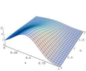
Figure 5.1: Vector probability distribution $\Phi^{V}(z,\mathbf{q}_{\perp})$ that three valence quarks leave the fraction $z$ of the baryon momentum and transverse momentum $\mathbf{q}_{\perp}$ to the quark-antiquark pair(s) in the relativistic (left) and non-relativistic (right) cases plotted in units of $M$ and normalized to unity for $z=\mathbf{q}_{\perp}=0$.

Relativistic corrections (quark angular momentum) clearly shift the bump in the probability distribution to smaller values of $z$ meaning that it leaves less longitudinal momentum fraction to the quark-antiquark pair(s). This can be easily understood from the shape of the discrete-level wave function $h(p)$ and $j(p)$, see Fig. 3.5. While the $s$-wave $h(p)$ is maximum at $p=0$, the $p$-wave $j(p)$ has a node. The maximum value of the latter is then obtained for non-vanishing $p$. Relativistic valence quarks then need more momentum than non-relativistic ones explaining the fact that less momentum is left for the quark-antiquark pair(s) in the relativistic case compared to the non-relativistic one.

In the following we give the integrals appearing in each Fock sector and the numerical values obtained for them. In the evaluation of the scalar overlap integrals we have used the constituent quark mass $M=345$ MeV, the Pauli-Villars mass $M_{\textrm{PV}}=556.8$ MeV for the regularization of (3.61)-(3.65), (3.67)-(3.79) and of (3.82)-(3.93) and the baryon mass $\mathcal{M}=1207$ MeV as it follows for the “classical” mass in the mean field approximation [114].

5.3.1 $3Q$ scalar integral

In the $3Q$ sector there is no quark-antiquark pair and thus only one integral is involved. It corresponds to the valence quark distribution without momentum left to the sea $\Phi^{V}(0,0)$. Notice that we have the freedom to choose the normalization of the discrete-level wave functions $h$ and $j$. In other words we have the freedom to choose in particular

$$\Phi^{V}(0,0)=1.$$ (5.13)

Since the relativistic and non-relativistic vector valence quark distributions have different expressions the normalization $\Phi^{V}(0,0)=1$ implies different normalizations for $h$ and $h_{NR}$. Diakonov and Petrov commented in [76] that the lower component $j(p)$ is “substantially” smaller than the upper one $h(p)$. More quantitatively it turned out that the $j(p)$ contribution to the normalization of the discrete-level wave function $\psi_{\textrm{lev}}(\mathbf{p})$ is still 20% (result in accordance with [149]). This with the combinatoric factors in eq. (LABEL:Phi) shows that taking the lower component $j$ into account can have a non-negligible impact on the estimations. The nucleon is thus definitely a relativistic system.

5.3.2 $5Q$ scalar integrals

In the $5Q$ sector there is one quark-antiquark pair. Contractions given by the direct diagram lead to three different integrals $J=\pi\pi,33,\sigma\sigma$. Only the scalar-to-scalar $\Sigma^{\dagger}\Sigma$ and pseudoscalar-to-pseudoscalar $\Pi^{\dagger}\Pi$ transitions are allowed.

In the non-relativistic case we have obtained

$$K^{V}_{\pi\pi,NR}=0.06237,\qquad K^{V}_{33,NR}=0.02842,\qquad K^{V}_{\sigma\sigma,NR}=0.03731$$ (5.14)

while in the relativistic case we have obtained

$$K^{V}_{\pi\pi}=0.03652,\qquad K^{V}_{33}=0.01975,\qquad K^{V}_{\sigma\sigma}=0.01401.$$ (5.15)

As one can expect from the comparison of both probability distributions in Fig. 5.1 relativistic corrections reduce strongly (about one half) the values of the $5Q$ scalar overlap integrals.

Contractions given by the exchange diagram lead to seven different integrals $J=1$-$7$ in the non-relativistic limit

$$K_{1}=0.00560,\qquad K_{2}=0.00968,\qquad K_{3}=-0.00077,\qquad K_{4}=0.00470,$$

$$K_{5}=0.00857,\qquad K_{6}=0.00423,\qquad K_{7}=0.00288.$$ (5.16)

Anticipating on the final results, these exchange contributions have only a small impact on the observables and can be reasonably neglected. That’s the reason why they haven’t been computed with relativistic corrections.

5.3.3 $7Q$ scalar integrals

In the $7Q$ sector there are two quark-antiquark pairs. Contractions given by the direct diagram give eight different integrals $J=\pi\pi\pi\pi,\pi\pi\pi\pi 2,\pi\pi 33,3333,\pi 3\pi 3,\sigma\sigma\pi\pi,\sigma\sigma 33,\sigma\sigma\sigma\sigma$. Since the $5Q$ sector taught us that relativistic effects are important these integrals have been evaluated with the relativistic valence probability distribution only

$$K^{V}_{\pi\pi\pi\pi}=0.00082,\qquad K^{V}_{\pi\pi\pi\pi 2}=0.00026,\qquad K^{V}_{\pi\pi 33}=0.00039,\qquad K^{V}_{3333}=0.00019,$$

$$K^{V}_{\pi 3\pi 3}=0.00017,\qquad K^{V}_{\sigma\sigma\pi\pi}=0.00027,\qquad K^{V}_{\sigma\sigma 33}=0.00012,\qquad K^{V}_{\sigma\sigma\sigma\sigma}=0.00009.$$ (5.17)

Even though these values are smaller than the $5Q$ exchange scalar integrals the contribution of the $7Q$ component is larger due to large combinatoric factors, see next section.

By analogy with the $5Q$ sector, exchange diagrams contributions are neglected and thus have not been computed.

5.4 Combinatoric results

Normalizations and vector matrix elements are linear combinations of the vector scalar overlap integrals. These specific combinations are obtained by contracting the baryon rotational wave functions with the vector operator. In the following we give for each multiplet the combinations obtained.

5.4.1 Octet baryons

Here are the expressions for the octet baryons normalization. They are obtained by contracting the octet baryon wave functions without any charge acting on the quark lines. The upper indices $3,5,7$ refer to the $3Q$, $5Q$ and $7Q$ Fock sectors.
The contributions to the octet normalization are

$$\mathcal{N}^{(3)}(B_{\bf 8}) = 9\,\Phi^{V}(0,0),$$ (5.18)

$$\mathcal{N}^{(5)}(B_{\bf 8}) = \frac{18}{5}\left(11K^{V}_{\pi\pi}+23K^{V}_{\sigma\sigma}\right),$$ (5.19)

$$\mathcal{N}^{(5)\textrm{exch}}(B_{\bf 8}) = \frac{-12}{5}\left(9K_{1}+4K_{3}+4K_{4}-17K_{6}-17K_{7}\right),$$ (5.20)

$$\mathcal{N}^{(7)}(B_{\bf 8}) = \frac{144}{5}\left(15K^{V}_{\pi\pi\pi\pi}+5K^{V}_{\pi\pi\pi\pi 2}+52K^{V}_{\sigma\sigma\pi\pi}+54K^{V}_{\sigma\sigma\sigma\sigma}\right).$$ (5.21)

In the $3Q$ sector there is no quark-antiquark pair and thus only valence quarks contribute to the vector charges

$$\alpha_{V,q_{\textrm{val}}}^{(3)}=18\,\Phi^{V}(0,0),\qquad\beta_{V,q_{\textrm{val}}}^{(3)}=9\,\Phi^{V}(0,0),\qquad\gamma_{V,q_{\textrm{val}}}^{(3)}=0.$$ (5.22)

In the $5Q$ sector one has for the direct diagram

$$\alpha_{V,q_{\textrm{val}}}^{(5)}=\frac{18}{5}\left(15K^{V}_{\pi\pi}+43K^{V}_{\sigma\sigma}\right),\quad\alpha_{V,q_{\textrm{s}}}^{(5)}=\frac{132}{5}\left(K^{V}_{\pi\pi}+K^{V}_{\sigma\sigma}\right),\quad\alpha_{V,\bar{q}}^{(5)}=\frac{6}{5}\left(K^{V}_{\pi\pi}+13K^{V}_{\sigma\sigma}\right),$$ (5.23)

$$\beta_{V,q_{\textrm{val}}}^{(5)}=\frac{72}{25}\left(12K^{V}_{\pi\pi}+25K^{V}_{\sigma\sigma}\right),\quad\beta_{V,q_{\textrm{s}}}^{(5)}=\frac{24}{25}\left(13K^{V}_{\pi\pi}+22K^{V}_{\sigma\sigma}\right),\quad\beta_{V,\bar{q}}^{(5)}=\frac{6}{25}\left(31K^{V}_{\pi\pi}+43K^{V}_{\sigma\sigma}\right),$$ (5.24)

$$\gamma_{V,q_{\textrm{val}}}^{(5)}=\frac{36}{25}\left(7K^{V}_{\pi\pi}+5K^{V}_{\sigma\sigma}\right),\quad\gamma_{V,q_{\textrm{s}}}^{(5)}=\frac{6}{25}\left(K^{V}_{\pi\pi}+49K^{V}_{\sigma\sigma}\right),\quad\gamma_{V,\bar{q}}^{(5)}=\frac{6}{25}\left(43K^{V}_{\pi\pi}+79K^{V}_{\sigma\sigma}\right).$$ (5.25)

Concerning the exchange diagram, since one cannot disentangle valence quarks from sea quarks we can decompose the parameters into quark $q_{\textrm{val+s}}$ and antiquark $\bar{q}$ contributions only

$$\alpha_{V,q_{\textrm{val+s}}}^{(5)\textrm{exch}} = \frac{-24}{25}\left(57K_{1}+22K_{3}+22K_{4}-101K_{6}-101K_{7}\right),$$ (5.26)

$$\alpha_{V,\bar{q}}^{(5)\textrm{exch}} = \frac{-48}{25}\left(6K_{1}+K_{3}+K_{4}-8K_{6}-8K_{7}\right),$$ (5.27)

$$\beta_{V,q_{\textrm{val+s}}}^{(5)\textrm{exch}} = \frac{-4}{25}\left(171K_{1}+91K_{3}+91K_{4}-353K_{6}-353K_{7}\right),$$ (5.28)

$$\beta_{V,\bar{q}}^{(5)\textrm{exch}} = \frac{-4}{25}\left(36K_{1}+31K_{3}+31K_{4}-98K_{6}-98K_{7}\right),$$ (5.29)

$$\gamma_{V,q_{\textrm{val+s}}}^{(5)\textrm{exch}} = \gamma_{V,\bar{q}}^{(5)\textrm{exch}}=\frac{-4}{25}\left(27K_{1}+17K_{3}+17K_{4}-61K_{6}-61K_{7}\right).$$ (5.30)

In the $7Q$ sector the combinations are

$$\alpha_{V,q_{\textrm{val}}}^{(7)} = \frac{48}{5}\left(49K^{V}_{\pi\pi\pi\pi}+38K^{V}_{\pi\pi\pi\pi 2}+200K^{V}_{\sigma\sigma\pi\pi}+285K^{V}_{\sigma\sigma\sigma\sigma}\right),$$ (5.31)

$$\alpha_{V,q_{\textrm{s}}}^{(7)} = \frac{48}{5}\left(47K^{V}_{\pi\pi\pi\pi}+2K^{V}_{\pi\pi\pi\pi 2}+144K^{V}_{\sigma\sigma\pi\pi}+99K^{V}_{\sigma\sigma\sigma\sigma}\right),$$ (5.32)

$$\alpha_{V,\bar{q}}^{(7)} = \frac{96}{5}\left(3K^{V}_{\pi\pi\pi\pi}+5K^{V}_{\pi\pi\pi\pi 2}+16K^{V}_{\sigma\sigma\pi\pi}+30K^{V}_{\sigma\sigma\sigma\sigma}\right),$$ (5.33)

$$\beta_{V,q_{\textrm{val}}}^{(7)} = \frac{48}{25}\left(181K^{V}_{\pi\pi\pi\pi}+41K^{V}_{\pi\pi\pi\pi 2}+626K^{V}_{\sigma\sigma\pi\pi}+618K^{V}_{\sigma\sigma\sigma\sigma}\right),$$ (5.34)

$$\beta_{V,q_{\textrm{s}}}^{(7)} = \frac{96}{25}\left(61K^{V}_{\pi\pi\pi\pi}+22K^{V}_{\pi\pi\pi\pi 2}+201K^{V}_{\sigma\sigma\pi\pi}+198K^{V}_{\sigma\sigma\sigma\sigma}\right),$$ (5.35)

$$\beta_{V,\bar{q}}^{(7)} = \frac{96}{25}\left(39K^{V}_{\pi\pi\pi\pi}+5K^{V}_{\pi\pi\pi\pi 2}+124K^{V}_{\sigma\sigma\pi\pi}+102K^{V}_{\sigma\sigma\sigma\sigma}\right),$$ (5.36)

$$\gamma_{V,q_{\textrm{val}}}^{(7)} = \frac{48}{25}\left(83K^{V}_{\pi\pi\pi\pi}-2K^{V}_{\pi\pi\pi\pi 2}+238K^{V}_{\sigma\sigma\pi\pi}+129K^{V}_{\sigma\sigma\sigma\sigma}\right),$$ (5.37)

$$\gamma_{V,q_{\textrm{s}}}^{(7)} = \frac{48}{25}\left(31K^{V}_{\pi\pi\pi\pi}+32K^{V}_{\pi\pi\pi\pi 2}+146K^{V}_{\sigma\sigma\pi\pi}+243K^{V}_{\sigma\sigma\sigma\sigma}\right),$$ (5.38)

$$\gamma_{V,\bar{q}}^{(7)} = \frac{288}{25}\left(19K^{V}_{\pi\pi\pi\pi}+5K^{V}_{\pi\pi\pi\pi 2}+64K^{V}_{\sigma\sigma\pi\pi}+62K^{V}_{\sigma\sigma\sigma\sigma}\right).$$ (5.39)

One can easily check that the obvious sum rules for the proton

$$\int\mathrm{d}z\,[u(z)-\bar{u}(z)]=2,\qquad\int\mathrm{d}z\,[d(z)-\bar{d}(z)]=1,\qquad\int\mathrm{d}z\,[s(z)-\bar{s}(z)]=0$$ (5.40)

are satisfied separately in each sector. They are translated in our parametrization as follows

$$\alpha_{V,q_{\textrm{val}}}^{(i)}+\alpha_{V,q_{\textrm{s}}}^{(i)}-\alpha_{V,\bar{q}}^{(i)}=2\mathcal{N}^{(i)}(B_{\bf 8}),\quad\beta_{V,q_{\textrm{val}}}^{(i)}+\beta_{V,q_{\textrm{s}}}^{(i)}-\beta_{V,\bar{q}}^{(i)}=\mathcal{N}^{(i)}(B_{\bf 8}),\quad\gamma_{V,q_{\textrm{val}}}^{(i)}+\gamma_{V,q_{\textrm{s}}}^{(i)}-\gamma_{V,\bar{q}}^{(i)}=0\quad\forall i.$$ (5.41)

5.4.2 Decuplet baryons

Here are the expressions for the decuplet baryons normalization. They are obtained by contracting the decuplet baryon wave functions without any charge acting on the quark lines. The upper indices $i=3,5$ refer to the $3Q$ and $5Q$ Fock sectors while the lower ones $3/2,1/2$ refer to the $z$-component of the decuplet baryon spin. Notice that in the $5Q$ sector only direct contributions are given. In our study of exchange diagrams only octet and antidecuplet were considered. Since the conclusion is that exchange contributions are negligible we did not compute them when we studied the decuplet.
The contributions to the decuplet normalization are

$$\mathcal{N}^{(3)}_{3/2}(B_{\bf 10}) = \mathcal{N}^{(3)}_{1/2}(B_{\bf 10})=\frac{18}{5}\,\Phi^{V}(0,0),$$ (5.42)

$$\mathcal{N}^{(5)}_{3/2}(B_{\bf 10}) = \frac{9}{5}\left(15K^{V}_{\pi\pi}-6K^{V}_{33}+17K^{V}_{\sigma\sigma}\right),$$ (5.43)

$$\mathcal{N}^{(5)}_{1/2}(B_{\bf 10}) = \frac{9}{5}\left(11K^{V}_{\pi\pi}+6K^{V}_{33}+17K^{V}_{\sigma\sigma}\right).$$ (5.44)

In the $3Q$ sector there is no quark-antiquark pair and thus only valence quarks contribute to the vector charges

$$\alpha^{\prime(3)}_{V,q_{\textrm{val}},3/2}=\alpha^{\prime(3)}_{V,q_{\textrm{val}},1/2}=\frac{18}{5}\,\Phi^{V}(0,0),\qquad\beta^{\prime(3)}_{V,q_{\textrm{val}},3/2}=\beta^{\prime(3)}_{V,q_{\textrm{val}},1/2}=0.$$ (5.45)

In the $5Q$ sector one has

$$\alpha^{\prime(5)}_{V,q_{\textrm{val}},3/2}=\frac{9}{20}\left(33K^{V}_{\pi\pi}-6K^{V}_{33}+67K^{V}_{\sigma\sigma}\right),\quad\alpha^{\prime(5)}_{V,q_{\textrm{s}},3/2}=\frac{3}{20}\left(57K^{V}_{\pi\pi}-30K^{V}_{33}+19K^{V}_{\sigma\sigma}\right),$$

$$\alpha^{\prime(5)}_{V,\bar{q},3/2}=\frac{-6}{5}\left(3K^{V}_{\pi\pi}-3K^{V}_{33}-2K^{V}_{\sigma\sigma}\right),$$ (5.46)

$$\alpha^{\prime(5)}_{V,q_{\textrm{val}},1/2}=\frac{9}{20}\left(29K^{V}_{\pi\pi}+6K^{V}_{33}+67K^{V}_{\sigma\sigma}\right),\quad\alpha^{\prime(5)}_{V,q_{\textrm{s}},1/2}=\frac{3}{20}\left(37K^{V}_{\pi\pi}+30K^{V}_{33}+19K^{V}_{\sigma\sigma}\right),$$

$$\alpha^{\prime(5)}_{V,\bar{q},1/2}=\frac{-6}{5}\left(K^{V}_{\pi\pi}+3K^{V}_{33}-2K^{V}_{\sigma\sigma}\right),$$ (5.47)

$$\beta^{\prime(5)}_{V,q_{\textrm{val}},3/2}=\frac{9}{20}\left(27K^{V}_{\pi\pi}-18K^{V}_{33}+K^{V}_{\sigma\sigma}\right),\quad\beta^{\prime(5)}_{V,q_{\textrm{s}},3/2}=\frac{3}{20}\left(3K^{V}_{\pi\pi}+6K^{V}_{33}+49K^{V}_{\sigma\sigma}\right),$$

$$\beta^{\prime(5)}_{V,\bar{q},3/2}=\frac{3}{5}\left(21K^{V}_{\pi\pi}-12K^{V}_{33}+13K^{V}_{\sigma\sigma}\right),$$ (5.48)

$$\beta^{\prime(5)}_{V,q_{\textrm{val}},1/2}=\frac{9}{20}\left(15K^{V}_{\pi\pi}+18K^{V}_{33}+K^{V}_{\sigma\sigma}\right),\quad\beta^{\prime(5)}_{V,q_{\textrm{s}},1/2}=\frac{3}{20}\left(7K^{V}_{\pi\pi}-6K^{V}_{33}+49K^{V}_{\sigma\sigma}\right),$$

$$\beta^{\prime(5)}_{V,\bar{q},1/2}=\frac{3}{5}\left(13K^{V}_{\pi\pi}+12K^{V}_{33}+13K^{V}_{\sigma\sigma}\right).$$ (5.49)

The $7Q$ sector of the decuplet has not been computed due to its far bigger complexity.

One can easily check that the obvious sum rules for $\Delta^{++}$

$$\int\mathrm{d}z\,[u(z)-\bar{u}(z)]=3,\qquad\int\mathrm{d}z\,[d(z)-\bar{d}(z)]=0,\qquad\int\mathrm{d}z\,[s(z)-\bar{s}(z)]=0$$ (5.50)

are satisfied separately in each sector. They are translated in our parametrization as follows

$$\alpha^{\prime(i)}_{V,q_{\textrm{val}},J}+\alpha^{\prime(i)}_{V,q_{\textrm{s}},J}-\alpha^{\prime(i)}_{V,\bar{q},J}=\mathcal{N}^{(i)}_{J}(B_{\bf 10}),\quad\beta^{\prime(i)}_{V,q_{\textrm{val}},J}+\beta^{\prime(i)}_{V,q_{\textrm{s}},J}-\beta^{\prime(i)}_{V,\bar{q},J}=0\quad\forall i\textrm{ and }J=3/2,1/2.$$ (5.51)

Let us emphasize an interesting observation. If the decuplet was made of three quarks only then one would have the following relation between spin-3/2 and spin-1/2 vector contributions

$$V_{3/2}=V_{1/2}.$$ (5.52)

This picture presents the $\Delta$ as a spherical particle. Things change in the $5Q$ sector. One notices directly that the relations are broken by a unique structure $(K^{V}_{\pi\pi}-3K^{V}_{33})$ in the vector case and normalizations. Going back to the definition of those integrals this amounts in fact to a structure like $(q^{2}-3q_{z}^{2})$ coming from the coupling to pions in $p$ waves. This naturally reminds the expression of a quadrupole

$$Q_{ij}=\int\mathrm{d}^{3}r\,\rho(\mathbf{r})\,(3r_{i}r_{j}-r^{2}\delta_{ij})$$ (5.53)

specified to the component $i=j=z$. Remarkably the present approach shows explicitly that the pion field is responsible for the deviation of the $\Delta$ from spherical symmetry. This discussion will be resumed in the chapter dedicated to magnetic moments, especially concerning the $\gamma N\Delta$ transition.

5.4.3 Antidecuplet baryons

Here are the expressions for the antidecuplet baryons normalization. They are obtained by contracting the antidecuplet baryon wave functions without any charge acting on the quark lines. The upper indices $5,7$ refer to the $5Q$ and $7Q$ Fock sectors.
The contributions to the antidecuplet normalization are

$$\mathcal{N}^{(5)}(B_{\bf\overline{10}}) = \frac{36}{5}\left(K^{V}_{\pi\pi}+K^{V}_{\sigma\sigma}\right),$$ (5.54)

$$\mathcal{N}^{(5)\textrm{exch}}(B_{\bf\overline{10}}) = \frac{-12}{5}\left(K_{3}+K_{4}-2K_{6}-2K_{7}\right),$$ (5.55)

$$\mathcal{N}^{(7)}(B_{\bf\overline{10}}) = \frac{72}{5}\left(9K^{V}_{\pi\pi\pi\pi}+K^{V}_{\pi\pi\pi\pi 2}+26K^{V}_{\sigma\sigma\pi\pi}+18K^{V}_{\sigma\sigma\sigma\sigma}\right).$$ (5.56)

In the $5Q$ sector one has for the direct diagram

$$\alpha^{\prime\prime(5)}_{V,q_{\textrm{val}}}=\frac{18}{5}\left(K^{V}_{\pi\pi}+K^{V}_{\sigma\sigma}\right),\quad\alpha^{\prime\prime(5)}_{V,q_{\textrm{s}}}=\frac{6}{5}\left(K^{V}_{\pi\pi}+K^{V}_{\sigma\sigma}\right),\quad\alpha^{\prime\prime(5)}_{V,\bar{q}}=\frac{-12}{5}\left(K^{V}_{\pi\pi}+K^{V}_{\sigma\sigma}\right),$$ (5.57)

$$\beta^{\prime\prime(5)}_{V,q_{\textrm{val}}}=\frac{18}{5}\left(K^{V}_{\pi\pi}+K^{V}_{\sigma\sigma}\right),\quad\beta^{\prime\prime(5)}_{V,q_{\textrm{s}}}=\frac{6}{5}\left(K^{V}_{\pi\pi}+K^{V}_{\sigma\sigma}\right),\quad\beta^{\prime\prime(5)}_{V,\bar{q}}=\frac{24}{5}\left(K^{V}_{\pi\pi}+K^{V}_{\sigma\sigma}\right).$$ (5.58)

The $5Q$ exchange diagram gives

$$\alpha^{\prime\prime(5)\textrm{exch}}_{V,q_{\textrm{val+s}}} = \frac{-8}{5}\left(K_{3}+K_{4}-2K_{6}-2K_{7}\right),$$ (5.59)

$$\alpha^{\prime\prime(5)\textrm{exch}}_{V,\bar{q}} = \frac{4}{5}\left(K_{3}+K_{4}-2K_{6}-2K_{7}\right),$$ (5.60)

$$\beta^{\prime\prime(5)\textrm{exch}}_{V,q_{\textrm{val+s}}} = \beta^{\prime\prime(5)\textrm{exch}}_{V,\bar{q}}=\frac{-8}{5}\left(K_{3}+K_{4}-2K_{6}-2K_{7}\right).$$ (5.61)

Compared to octet and decuplet baryons, antidecuplet baryons have a rather simple $5Q$ component. This is of course related to the fact that there is no $3Q$ component. The minimal content of a baryon is simple while higher Fock states introduce more complicated structures.

In the $7Q$ sector one has

$$\alpha^{\prime\prime(7)}_{V,q_{\textrm{val}}} = \frac{12}{5}\left(22K^{V}_{\pi\pi\pi\pi}+5K^{V}_{\pi\pi\pi\pi 2}+68K^{V}_{\sigma\sigma\pi\pi}+51K^{V}_{\sigma\sigma\sigma\sigma}\right),$$ (5.62)

$$\alpha^{\prime\prime(7)}_{V,q_{\textrm{s}}} = \frac{12}{5}\left(17K^{V}_{\pi\pi\pi\pi}+2K^{V}_{\pi\pi\pi\pi 2}+42K^{V}_{\sigma\sigma\pi\pi}+27K^{V}_{\sigma\sigma\sigma\sigma}\right),$$ (5.63)

$$\alpha^{\prime\prime(7)}_{V,\bar{q}} = \frac{-12}{5}\left(15K^{V}_{\pi\pi\pi\pi}-K^{V}_{\pi\pi\pi\pi 2}+46K^{V}_{\sigma\sigma\pi\pi}+30K^{V}_{\sigma\sigma\sigma\sigma}\right),$$ (5.64)

$$\beta^{\prime\prime(7)}_{V,q_{\textrm{val}}} = \frac{12}{5}\left(32K^{V}_{\pi\pi\pi\pi}+K^{V}_{\pi\pi\pi\pi 2}+88K^{V}_{\sigma\sigma\pi\pi}+57K^{V}_{\sigma\sigma\sigma\sigma}\right),$$ (5.65)

$$\beta^{\prime\prime(7)}_{V,q_{\textrm{s}}} = \frac{12}{5}\left(19K^{V}_{\pi\pi\pi\pi}+2K^{V}_{\pi\pi\pi\pi 2}+62K^{V}_{\sigma\sigma\pi\pi}+45K^{V}_{\sigma\sigma\sigma\sigma}\right),$$ (5.66)

$$\beta^{\prime\prime(7)}_{V,\bar{q}} = \frac{36}{5}\left(17K^{V}_{\pi\pi\pi\pi}+K^{V}_{\pi\pi\pi\pi 2}+50K^{V}_{\sigma\sigma\pi\pi}+34K^{V}_{\sigma\sigma\sigma\sigma}\right).$$ (5.67)

One can easily check that the obvious sum rules for $\Theta^{+}$

$$\int\mathrm{d}z\,[u(z)-\bar{u}(z)]=2,\qquad\int\mathrm{d}z\,[d(z)-\bar{d}(z)]=2,\qquad\int\mathrm{d}z\,[s(z)-\bar{s}(z)]=-1$$ (5.68)

are satisfied separately in each sector. They are translated in our parametrization as follows

$$\alpha^{\prime\prime(i)}_{V,q_{\textrm{val}}}+\alpha^{\prime\prime(i)}_{V,q_{\textrm{s}}}-\alpha^{\prime\prime(i)}_{V,\bar{q}}=\mathcal{N}^{(i)}(B_{\bf\overline{10}}),\qquad\beta^{\prime\prime(i)}_{V,q_{\textrm{val}}}+\beta^{\prime\prime(i)}_{V,q_{\textrm{s}}}-\beta^{\prime\prime(i)}_{V,\bar{q}}=0\qquad\forall i.$$ (5.69)

5.5 Numerical results and discussion

Let us start the discussion of our results with the normalizations. They allow us to estimate which fraction of proton is actually made of $3Q$, $5Q$ and $7Q$.

In the non-relativistic limit $j(p)=0$ we have computed up to $5Q$ sector the octet composition, see Table 5.1. In this limit the proton consist of $2/3$ state with three quarks and $1/3$ state with five quarks. The exchange diagram does not change significantly these ratios and contribute only up to $1\%$. Already at this stage we can expect reasonably that neglecting the exchange diagram would not alter noticeably the results.

Table 5.1: Non-relativistic octet baryons fractions with and without exchange diagram contribution.

dir	$3Q\equiv\frac{\mathcal{N}^{(3)}(B)}{\mathcal{N}^{(3)}(B)+\mathcal{N}^{(5)}(B)}$	$5Q\equiv\frac{\mathcal{N}^{(5)}(B)}{\mathcal{N}^{(3)}(B)+\mathcal{N}^{(5)}(B)}$
$B_{\bf 8}$	$65\%$	$35\%$
dir+exch	$3Q\equiv\frac{\mathcal{N}^{(3)}(B)}{\mathcal{N}^{(3)}(B)+\mathcal{N}^{(5)}(B)+\mathcal{N}^{(5)\textrm{exch}}(B)}$	$5Q\equiv\frac{\mathcal{N}^{(5)}(B)+\mathcal{N}^{(5)\textrm{exch}}(B)}{\mathcal{N}^{(3)}(B)+\mathcal{N}^{(5)}(B)+\mathcal{N}^{(5)\textrm{exch}}(B)}$
$B_{\bf 8}$	$64\%$	$36\%$

In Table 5.2 we give the composition of octet and decuplet baryons still up to the $5Q$ sector but with the relativistic correction $j(p)\neq 0$. Let us first compare the relativistic result for the octet with the non-relativistic one. Quark angular momentum clearly reduces the impact of the $5Q$ component. The $5Q$ scalar overlap integrals being smaller in the relativistic case than in the non-relativistic one the conclusion drawn is not surprising. This effect is not negligible since the $5Q$ weight drops from 1/3 to less than 1/4. Let us compare now the octet and decuplet fractions. They appear to be quite similar but notice that the $J_{z}=1/2$ component of the decuplet has a slightly larger $5Q$ component than the $J_{z}=3/2$ one.

Table 5.2: Comparison of octet and decuplet baryons fractions up to the $5Q$ sector.

	$3Q\equiv\frac{\mathcal{N}^{(3)}(B)}{\mathcal{N}^{(3)}(B)+\mathcal{N}^{(5)}(B)}$	$5Q\equiv\frac{\mathcal{N}^{(5)}(B)}{\mathcal{N}^{(3)}(B)+\mathcal{N}^{(5)}(B)}$
$B_{\bf 8}$	$77.5\%$	$22.5\%$
$B_{\mathbf{10},3/2}$	$75\%$	$25\%$
$B_{\mathbf{10},1/2}$	$72.5\%$	$27.5\%$

A more precise description of baryons would involve the $7Q$ sector. By analogy with the $5Q$ sector of ordinary baryons, pentaquarks are expected to have a non-negligible $7Q$ component. In Table 5.3 one observes that the dominant component in pentaquarks is smaller ($\sim 60\%$) than the dominant one in ordinary baryons ($\sim 75\%$). This would indicate that when considering a pentaquark one should care more about higher Fock contributions than in ordinary baryons. Concerning these ordinary baryons, it is interesting to notice that the $7Q$ component is not that negligible since $7.5\%$ of the proton is a system with seven quarks. It is however not surprising that the adjunction of the $7Q$ sector reduces the weight of the other ones.

Table 5.3: Comparison of octet and antidecuplet baryons fractions up to the $7Q$ sector.

	$3Q\equiv\frac{\mathcal{N}^{(3)}(B)}{\mathcal{N}^{(3)}(B)+\mathcal{N}^{(5)}(B)+\mathcal{N}^{(7)}(B)}$	$5Q\equiv\frac{\mathcal{N}^{(5)}(B)}{\mathcal{N}^{(3)}(B)+\mathcal{N}^{(5)}(B)+\mathcal{N}^{(7)}(B)}$	$7Q\equiv\frac{\mathcal{N}^{(7)}(B)}{\mathcal{N}^{(3)}(B)+\mathcal{N}^{(5)}(B)+\mathcal{N}^{(7)}(B)}$
$B_{\mathbf{8}}$	$71.7\%$	$20.8\%$	$7.5\%$
$B_{\mathbf{\overline{10}}}$	$0\%$	$60.6\%$	$39.4\%$

We now proceed with our results concerning baryon vector content.

5.5.1 Octet content

The first Table 5.4 contains the non-relativistic contributions to proton vector charges

Table 5.4: Our non-relativistic vector content of the proton.

Vector	$u$		$d$		$s$
	$\bar{q}$	$q_{s}+q_{val}$	$\bar{q}$	$q_{s}+q_{val}$	$\bar{q}$	$q_{s}+q_{val}$
$3Q$	0	2	0	1	0	0
$3Q+5Q$ (dir)	0.123	2.123	0.140	1.140	0.086	0.086
$3Q+5Q$ (dir+exch)	0.125	2.125	0.143	1.143	0.087	0.087

while relativistic results can be found in Table 5.5. Since the $5Q$ component is larger in the non-relativistic it is not surprising to find more antiquarks in this limit. Exchange contributions are of order 1-2% and are thus clearly negligible. A coincidence makes that the non-relativistic proton up to the $5Q$ picture seems equivalent to the relativistic proton up to the $7Q$ picture concerning the vector properties.

Table 5.5: Our vector content of the proton compared with NQM.

Vector	$u$			$d$			$s$
	$\bar{q}$	$q_{s}$	$q_{val}$	$\bar{q}$	$q_{s}$	$q_{val}$	$\bar{q}$	$q_{s}$	$q_{val}$
NQM	0	0	2	0	0	1	0	0	0
$3Q$	0	0	2	0	0	1	0	0	0
$3Q+5Q$	0.078	0.130	1.948	0.091	0.080	1.012	0.055	0.015	0.040
$3Q+5Q+7Q$	0.125	0.202	1.924	0.145	0.128	1.017	0.088	0.028	0.060

Considering Fock states beyond the $3Q$ sector naturally generates antiquarks with the three flavors. As discussed previously the sea is not $SU(3)$ symmetric as sometimes assumed in models. $SU(3)$ symmetry does not force neither $\bar{q}$ and $q_{\textrm{s}}$ to be equal nor that the $u$, $d$ and $s$ sea to have the same magnitude. The population in the sea is affected by the population in the valence sector. They cannot be treated independently. Another interesting comment is that as also discussed previously, hidden flavor(s) can access to the valence level. Our computations show the existence of valence strange quarks in the proton. This simple observation can be used to understand the fact that even if the effective number of strange quarks $s-\bar{s}$ is zero the strange quark and antiquark distributions are not necessarily equal $s(z)-\bar{s}(z)\neq 0$ as revealed by experiments [148].

The corrections due to the $7Q$ component go in the same direction as the ones due to the $5Q$ component. The former are of course (and fortunately) small but not that negligible. Results are quantitatively but not qualitatively changed. While the $5Q$ component is essential in order to produce a sea contribution, exploratory studies do not need absolutely this $7Q$ component. Only a fine quantitative estimation would have to take it into account. The problem is that it is difficult to estimate the theoretical errors of the actual approach hitherto. Further work is thus needed.

Violation of Gottfried sum rule [52] allows one to study also the vector content of the sea. Experiments suggest that $\bar{d}$ is dominant over $\bar{u}$. This can physically be understood by considering some simple Pauli-blocking effect. Since there are already two valence $u$ quarks and only one valence $d$ quark in the proton, the presence of $\bar{d}d$ pair will be favored compared to $\bar{u}u$. The E866 collaboration [141] gives $\bar{d}-\bar{u}=0.118\pm 0.012$ while we have obtained $\bar{d}-\bar{u}=0.019$. We indeed confirm an excess of $\bar{d}$ over $\bar{u}$ but the magnitude is one order of magnitude too small.

5.5.2 Decuplet content

In Tables 5.6 and 5.7 one can find the $\Delta^{++}$ vector content with respectively $J_{z}=3/2,1/2$.

Table 5.6: Our vector content of the $\Delta^{++}$ with spin projection $J_{z}=3/2$ compared with NQM.

Vector	$u$			$d$			$s$
$J_{z}=3/2$	$\bar{q}$	$q_{s}$	$q_{val}$	$\bar{q}$	$q_{s}$	$q_{val}$	$\bar{q}$	$q_{s}$	$q_{val}$
NQM	0	0	3	0	0	0	0	0	0
$3Q$	0	0	3	0	0	0	0	0	0
$3Q+5Q$	0.072	0.193	2.879	0.089	0.029	0.060	0.089	0.029	0.060

Table 5.7: Our vector content of the $\Delta^{++}$ with spin projection $J_{z}=1/2$ compared with NQM.

Vector	$u$			$d$			$s$
$J_{z}=1/2$	$\bar{q}$	$q_{s}$	$q_{val}$	$\bar{q}$	$q_{s}$	$q_{val}$	$\bar{q}$	$q_{s}$	$q_{val}$
NQM	0	0	3	0	0	0	0	0	0
$3Q$	0	0	3	0	0	0	0	0	0
$3Q+5Q$	0.059	0.225	2.834	0.108	0.025	0.083	0.108	0.025	0.083

To the best of our knowledge there is no experimental results concerning the vector content of decuplet baryons. Our results can then be considered as just theoretical predictions, at least qualitatively. As discussed in the previous section, it is clear that eq. (5.52) is not satisfied indicating a deviation from spherical shape .

Note however that the $3Q$ sector reproduces all the octet and decuplet vector content predicted by NQM. Higher Fock sectors change these results by breaking explicitly $SU(6)$ symmetry.

5.5.3 Antidecuplet content

The study of the $7Q$ sector has mainly been motivated by the pentaquark. In previous results we have seen that the $5Q$ component of usual baryons has non-negligible and interesting effects on the vector quantities. In the same spirit, since there is no $3Q$ component in pentaquarks, it would be interesting to see what happens when considering the $7Q$ component. In Table 5.8 one can find the $\Theta^{+}$ vector content.

Table 5.8: Our vector content of the $\Theta^{+}$.

Vector	$u$			$d$			$s$
	$\bar{q}$	$q_{s}$	$q_{val}$	$\bar{q}$	$q_{s}$	$q_{val}$	$\bar{q}$	$q_{s}$	$q_{val}$
$5Q$	0	1/2	3/2	0	1/2	3/2	1	0	0
$5Q+7Q$	0.153	0.680	1.474	0.153	0.680	1.474	1.088	0.035	0.053

We did not provide a table with direct and exchange $5Q$ contributions. The minimal pentaquark content lies in the $5Q$ sector. This means that the structure is simple and is the same for both type of diagrams, emphi.e. the exchange diagram does not change the minimal vector content of pentaquarks. The sole restriction is that exchange diagram forbids a clear distinction between valence quarks and quarks from the sea.

The $7Q$ component introduces $\bar{u}$, $\bar{d}$ and $s$ in $\Theta^{+}$. In accordance with the normalizations this $7Q$ contribution has a stronger impact on pentaquarks than the $5Q$ contribution on ordinary baryons. A precise study of pentaquarks needs thus to take $7Q$ contributions into account.

Chapter 6 Axial charges

6.1 Introduction

The axial charges of a baryon are defined as forward matrix elements of the axial vector current

$$\langle B(p)|\bar{\psi}\gamma_{\mu}\gamma_{5}\lambda^{a}\psi|B(p)\rangle=g^{(a)}_{A}\bar{u}(p)\gamma_{\mu}\gamma_{5}u(p)$$ (6.1)

where $a=0,3,8$ and $\lambda^{3},\lambda^{8}$ are Gell-Mann matrices, $\lambda^{0}$ is just in this context the $3\times 3$ unit matrix. In principle we could add in the definition of the axial-vector operator $\bar{\psi}\gamma_{\mu}\gamma_{5}\lambda^{a}\psi$ a factor $g_{Aq}$ which is the quark axial-vector current coupling constant. As commonly assumed we use $g_{Aq}=1$, i.e. the same as for the structureless QCD quarks. These axial charges are related to the first moment of the longitudinally polarized quark distributions

$$g^{(3)}_{A}=\Delta u-\Delta d,\qquad g^{(8)}_{A}=\frac{1}{\sqrt{3}}(\Delta u+\Delta d-2\Delta s),\qquad g^{(0)}_{A}=\Delta u+\Delta d+\Delta s$$ (6.2)

where $\Delta q\equiv\int_{0}^{1}\mathrm{d}z\left[q_{+}(z)-q_{-}(z)+\bar{q}_{+}(z)-\bar{q}_{-}(z)\right]$ with $q=u,d,s$. Isovector $g_{A}^{(3)}$ and octet $g_{A}^{(8)}$ axial charges are independent of the renormalization point. On the contrary, the flavor singlet axial charge $g_{A}^{(0)}$ depends on the renormalization scale at which it is measured. Because of isospin symmetry we expect $g_{A}^{(3)}$ in proton to be equal to the axial charge of the transition $p^{+}_{\mathbf{8}}\to\pi^{+}n^{0}_{\mathbf{8}}$. We split the axial charges into valence quark, sea quark and antiquark contributions

$$\Delta q=\Delta q_{\textrm{val}}+\Delta q_{\textrm{sea}},\qquad\Delta q_{\textrm{sea}}=\Delta q_{\textrm{s}}+\Delta\bar{q}$$ (6.3)

where index s refers to the quarks in the sea pairs.

The axial charges can be understood as follows. They count the total number of quarks with spin aligned $q_{+}$ minus the total number of quarks with spin antialigned $q_{-}$ with the baryon spin, irrespective of their quark $q_{\textrm{val,s}}$ or antiquark $\bar{q}$ nature. The axial charges $\bar{q}\gamma_{\mu}\gamma_{5}q$ then give the contribution of quarks spin with flavor $q=u,d,s$ to the total baryon spin.

The proton polarized structure function $g_{1}^{p}(x)$ has been measured by EMC in 1987 [33]. The value obtained by the collaboration implies that only a small part of the nucleon spin is carried by quarks demonstrating that the Ellis-Jaffe Sum Rule (EJSR) [30] based on $\Delta s=\Delta\bar{s}=0$ did not hold true. This result was not anticipated in conventional quark models and is often referred to as the proton spin crisis in the literature, see e.g. the review [40]. Subsequent measurements at CERN and SLAC supported the initial EMC measurements and a global analysis [150] of these data suggested $\Delta s\approx-0.15$. It carries however with it an unknown theoretical uncertainty because DIS must be extrapolated to $x=0$ and an assumption of flavor $SU(3)$ symmetry must be invoked.

In DIS one is probing the baryon in IMF where the relativistic many-body problem is suitably described. There is consequently a significant change in the vector sum of quark spins, arising from relativistic effects due to internal quark motions. So $\Delta q$ measured in DIS has to be interpreted as the net spin polarization of quarks in the IMF which is different from the net spin vector sum of quark spins in the rest frame. The reason for this reduction of spin contribution can be ascribed to a negative spin contribution from the lower component of the Dirac spinor when the quark transversal motions are considered. A quantitative estimation of this effect can be obtained using the light-cone CQM. The results is that the correction is significative but not sufficient. The missing spin has thus to be carried by non-valence degrees of freedom, i.e. quark-antiquark pairs and gluons.

It is very important to study axial charges since a lot of physics is involved. Many ingredients have to be incorporated in a realistic model: relativistic quark description with orbital motion, non-valence degrees of freedom, strangeness, …We draw the attention to the fact that the values of $\Delta u$ and $\Delta d$ may have astrophysical knock-on effects [151]. A precise determination of their value is thus highly desired. Let us also note that axial charges are affected by the first-order flavor $SU(3)$ symmetry breaking while vector charges are safe as stated by the Ademollo-Gatto theorem [152]. Longitudinally polarized SIDIS [48] are subject to a growing interest as they provide an additional information on the spin structure of the nucleon compared to inclusive DIS measurements. They allow one to separate valence and sea contributions to the nucleon spin. Recent data suggest an asymmetry between $\Delta\bar{u}(x)$ and $\Delta\bar{d}(x)$ [48, 47, 49]. Flavor structure and spin structure of the nucleon sea are closely related [153]. All these points explain the interest in these quantities in both theoretical and experimental sides.

6.2 Axial charges on the light cone

Axial charges are obtained from the plus component of the axial-vector current operator $\bar{\psi}\gamma^{+}\gamma_{5}\psi$

$$\Delta q=\frac{1}{2P^{+}}\langle P,\frac{1}{2}|\bar{\psi}_{LC}\gamma^{+}\gamma_{5}\psi_{LC}|P,\frac{1}{2}\rangle.$$ (6.4)

Using the Melosh rotation one can see that $\Delta q_{LC}$ and $\Delta q_{NR}$ are related as follows [154]

$$\Delta q_{LC}=\langle M_{A}\rangle\Delta q_{NR}$$ (6.5)

where

$$M_{A}=\frac{(m_{q}+z_{3}\mathcal{M})^{2}-\mathbf{p}_{3\perp}^{2}}{(m_{q}+z_{3}\mathcal{M})^{2}+\mathbf{p}_{3\perp}^{2}}$$ (6.6)

and $\langle M_{A}\rangle$ is its expectation value

$$\langle M\rangle=\int\mathrm{d}^{3}p\,M|\Psi(p)|^{2}$$ (6.7)

with $\Psi(p)$ a simple normalized momentum wave function. The calculation with two different wave functions (harmonic oscillator and power-law fall off) gave $\langle M_{A}\rangle=0.75$ [155]. Relativity implies that quarks may have non-zero orbital angular momentum. The total baryon spin is thus not only due to quark spins but also to their orbital angular momentum.

In the IMF language one has to use the “good” components $\mu=0,3$ of the axial-vector current operator. This operator does not flip the spin but treats differently quarks with spin up and quarks with spin down. We have then $M^{\tau}_{\sigma}=(\sigma_{3})^{\tau}_{\sigma}$.

6.3 Scalar overlap integrals and quark distributions

From the expression (3.35) and if we concentrate on the spin part the contraction of two valence wave functions $F$ with the axial vector operator gives

$$F^{\dagger}(\sigma_{3})F\propto h^{2}(p)+2h(p)\frac{p_{z}}{|\mathbf{p}|}j(p)+\frac{2p_{z}^{2}-p^{2}}{p^{2}}j^{2}(p).$$ (6.8)

Like the vector operator the axial-vector operator does not flip quark spin. However it treats differently quarks with spin up and quarks with spin down. A quark with total angular momentum $J_{z}=+1/2$ may have orbital angular momentum $L_{z}=+1$ and has thus spin $S_{z}=-1/2$. Only the third term in (6.8) has components with $L_{z}\neq 0$ expressed by a factor $\mathbf{p}_{\perp}$. Since the spin for those components is opposed to the total angular momentum of the quark the sign in front of $p_{z}^{2}$ (no orbital angular momentum in the $z$ direction) is opposed to the one in front of $\mathbf{p}_{\perp}^{2}$ (non-zero orbital angular momentum in the $z$ direction). The structure of the third term in the axial sector is thus $p_{z}^{2}-\mathbf{p}_{\perp}^{2}=2p_{z}^{2}-p^{2}$ while it was $p_{z}^{2}+\mathbf{p}_{\perp}^{2}=p^{2}$ in the vector sector.

The axial valence quark distribution is obtained by the multiplication of two factors with structure (5.10) where the momentum is respectively $p_{1}$ and $p_{2}$ and a third factor with structure (6.8) and momentum $p_{3}$. The expansion gives the following function $D$

$$D^{A}(p_{1},p_{2},p_{3})=h^{2}(p_{1})h^{2}(p_{2})h^{2}(p_{3})+6h^{2}(p_{1})h^{2}(p_{2})\left[h(p_{3})\frac{p_{3z}}{|\mathbf{p}_{3}|}j(p_{3})\right]+h^{2}(p_{1})h^{2}(p_{2})\frac{2p_{3z}^{2}+p_{3}^{2}}{p_{3}^{2}}j^{2}(p_{3})$$

$$+12h^{2}(p_{1})\left[h(p_{2})\frac{p_{2z}}{|\mathbf{p}_{2}|}j(p_{2})\right]\left[h(p_{3})\frac{p_{3z}}{|\mathbf{p}_{3}|}j(p_{3})\right]+4h^{2}(p_{1})\left[h(p_{2})\frac{p_{2z}}{|\mathbf{p}_{2}|}j(p_{2})\right]\frac{2p_{3z}^{2}+p_{3}^{2}}{p_{3}^{2}}j^{2}(p_{3})$$

$$+8\left[h(p_{1})\frac{p_{1z}}{|\mathbf{p}_{1}|}j(p_{1})\right]\left[h(p_{2})\frac{p_{2z}}{|\mathbf{p}_{2}|}j(p_{2})\right]\left[h(p_{3})\frac{p_{3z}}{|\mathbf{p}_{3}|}j(p_{3})\right]+h^{2}(p_{1})j^{2}(p_{2})\frac{4p_{3z}^{2}-p_{3}^{2}}{p_{3}^{2}}j^{2}(p_{3})$$ (6.9)

$$+4\left[h(p_{1})\frac{p_{1z}}{|\mathbf{p}_{1}|}j(p_{1})\right]\left[h(p_{2})\frac{p_{2z}}{|\mathbf{p}_{2}|}j(p_{2})\right]\frac{2p_{3z}^{2}+p_{3}^{2}}{p_{3}^{2}}j^{2}(p_{3})+2\left[h(p_{1})\frac{p_{1z}}{|\mathbf{p}_{1}|}j(p_{1})\right]j^{2}(p_{2})\frac{4p_{3z}^{2}-p_{3}^{2}}{p_{3}^{2}}j^{2}(p_{3})$$

$$+j^{2}(p_{1})j^{2}(p_{2})\frac{2p_{3z}^{2}-p_{3}^{2}}{p_{3}^{2}}j^{2}(p_{3}).$$

that is needed in the expression of the valence quark distribution (3.59). In the non-relativistic limit $j=0$ this function $D$ is reduced to

$$D^{A}_{NR}(p_{1},p_{2},p_{3})=D^{V}_{NR}(p_{1},p_{2},p_{3})=h^{2}(p_{1})h^{2}(p_{2})h^{2}(p_{3}).$$ (6.10)

The valence probability distribution $\Phi^{I}(z,\mathbf{q}_{\perp})$ is then obtained by integration over the valence quark momenta, see eq. (3.59) and is depicted in Fig. 6.1 in vector $I=V$ and axial $I=A$ cases.

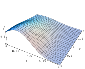
Figure 6.1: Probability distribution $\Phi^{I}(z,\mathbf{q}_{\perp})$ that three valence quarks leave the fraction $z$ of the baryon momentum and transverse momentum $\mathbf{q}_{\perp}$ to the quark-antiquark pair(s) in the vector $I=V$ (left) and axial $I=A$ (right) cases plotted in units of $M$ and normalized to $\Phi^{V}(0,0)=1$.

While in the non-relativistic limit valence probability distributions are the same, relativistic corrections (quark angular momentum) are different in vector and axial cases. This is of course due to the difference in structure between (6.8) and (5.10).

In the following we give the integrals appearing in each Fock sector and the numerical values obtained for them. In the evaluation of the scalar overlap integrals we have used the constituent quark mass $M=345$ MeV, the Pauli-Villars mass $M_{\textrm{PV}}=556.8$ MeV for the regularization of (3.61)-(3.65), (3.67)-(3.79) and of (3.82)-(3.93) and the baryon mass $\mathcal{M}=1207$ MeV as it follows for the “classical” mass in the mean field approximation [114].

6.3.1 $3Q$ scalar integral

In the $3Q$ sector there is no quark-antiquark pair and thus only one integral is involved. It corresponds to the valence quark distribution without momentum left to the sea $\Phi^{A}(0,0)$. We remind that the normalization chosen for $h(p)$ and $j(p)$ is such that $\Phi^{V}(0,0)=1$. From Figure 6.1 one can see that $\Phi^{A}(0,0)<1$. The precise value is

$$\Phi^{A}(0,0)=0.86115.$$ (6.11)

This means that in a simple $3Q$ picture all NQM axial charges have to be multiplied by this factor. Not surprisingly this is the same prescription as the one encountered in a standard light-cone approach based on Melosh rotation. Valence quark motion is a relativistic effect and is responsible for a noticeable reduction of NQM predictions. The Melosh factor 3/4 is of course smaller than the one we have obtained because of the function $h(p)$ absent in the Melosh approach but necessary in a fully relativistic treatment.

The NQM is recovered in the $3Q$ non-relativistic limit only where the three valence quarks have no angular orbital momentum and thus $\Phi^{A}_{NR}(0,0)=\Phi^{V}_{NR}(0,0)=1$.

6.3.2 $5Q$ scalar integrals

In the $5Q$ sector there is one quark-antiquark pair. Contractions given by the direct diagram give four different integrals $J=\pi\pi,33,\sigma\sigma,3\sigma$. If the axial-vector operator acts on valence quarks, the quark-antiquark pair is not affected and thus the integrals present the vector structure for the sea. If the axial-vector operator acts on the sea, the valence quarks are not affected and the vector valence probability distribution has to be used. The integrals present a new structure for the sea which describes the transition scalar$\leftrightarrow$pseudoscalar imposed by the “pseudo” feature of the axial-vector operator.

In the non-relativistic case, since $\Phi^{A}_{NR}=\Phi^{V}_{NR}$ only one new integrals has to be computed

$$K^{A}_{\pi\pi,NR}=K^{V}_{\pi\pi,NR},\quad K^{A}_{33,NR}=K^{V}_{33,NR},\quad K^{A}_{\sigma\sigma,NR}=K^{V}_{\sigma\sigma,NR},\quad K^{V}_{3\sigma,NR}=0.03338$$ (6.12)

while in the relativistic case there are four new integrals

$$K^{A}_{\pi\pi}=0.03003,\qquad K^{A}_{33}=0.01628,\qquad K^{A}_{\sigma\sigma}=0.01121,\qquad K^{V}_{3\sigma}=0.01626.$$ (6.13)

Let us have a look to the ratios $K^{A}_{J}/K^{V}_{J}$ with $J=\pi\pi,33,\sigma\sigma$

$$\frac{K^{A}_{\pi\pi}}{K^{V}_{\pi\pi}}=0.82228,\qquad\frac{K^{A}_{33}}{K^{V}_{33}}=0.82458,\qquad\frac{K^{A}_{\sigma\sigma}}{K^{V}_{\sigma\sigma}}=0.80039.$$ (6.14)

The reduction is of the same order as in the $3Q$ sector. It is however different from one structure to another due to the details of the valence probability distributions.

Contractions given by the exchange diagram lead to thirteen different integrals $J=1$-$13$. Since these integrals are obtained in the non-relativistic limit only six are new $J=8$-$13$

$$K_{8}=0.00431,\qquad K_{9}=0.00309,\qquad K_{10}=0.00693,$$

$$K_{11}=0.00172,\qquad K_{12}=0.00570,\qquad K_{13}=0.00230.$$ (6.15)

All exchange integrals are one order of magnitude smaller than the direct ones. This is however not sufficient to conclude that they can be neglected. Combinatoric factors play an important role as we have seen in the vector case.

6.3.3 $7Q$ scalar integrals

In the $7Q$ sector there are two quark-antiquark pairs. Contractions given by the direct diagram give twelve different integrals $J=\pi\pi\pi\pi,\pi\pi\pi\pi 2,\pi\pi 33,3333,\pi 3\pi 3,\sigma\sigma\pi\pi,\sigma\sigma 33,\sigma\sigma\sigma\sigma,\pi\pi 3\sigma,333\sigma,\pi 3\pi\sigma,\sigma\sigma 3\sigma$. Like in the $5Q$ sector all vector structures of the sea are associated with the axial valence probability distribution. One then gets eight integrals. The last four structures are the new axial structures of the sea

$$K^{A}_{\pi\pi\pi\pi}=0.00066,\qquad K^{A}_{\pi\pi\pi\pi 2}=0.00021,\qquad K^{A}_{\pi\pi 33}=0.00031,\qquad K^{A}_{3333}=0.00015,$$ (6.16)

$$K^{A}_{\pi 3\pi 3}=0.00013,\qquad K^{A}_{\sigma\sigma\pi\pi}=0.00021,\qquad K^{A}_{\sigma\sigma 33}=0.00010,\qquad K^{A}_{\sigma\sigma\sigma\sigma}=0.00007,$$ (6.17)

$$K^{V}_{\pi\pi 3\sigma}=0.00031,\qquad K^{V}_{333\sigma}=0.00014,\qquad K^{V}_{\pi 3\pi\sigma}=0.00011,\qquad K^{V}_{\sigma\sigma 3\sigma}=0.00010.$$ (6.18)

By analogy with the $5Q$ sector exchange diagram contributions are neglected and thus have not been computed.

6.4 Combinatoric Results

Axial matrix elements are linear combinations of the axial scalar overlap integrals. These specific combinations are obtained by contracting the baryon rotational wave functions with the axial-vector operator. In the following we give for each multiplet the combinations obtained.

6.4.1 Octet baryons

In the $3Q$ sector there is no quark-antiquark pair and thus only valence quarks contribute to the charges

$$\alpha_{A,q_{\textrm{val}}}^{(3)}=12\,\Phi^{A}(0,0),\qquad\beta_{A,q_{\textrm{val}}}^{(3)}=-3\,\Phi^{A}(0,0),\qquad\gamma_{A,q_{\textrm{val}}}^{(3)}=0.$$ (6.19)

In the $5Q$ sector one has for the direct diagram

$$\alpha_{A,q_{\textrm{val}}}^{(5)}=\frac{6}{5}\left(29K^{A}_{\pi\pi}+2K^{A}_{33}+91K^{A}_{\sigma\sigma}\right),\quad\alpha_{A,q_{\textrm{s}}}^{(5)}=\frac{-168}{5}\,K^{V}_{3\sigma},\quad\alpha_{A,\bar{q}}^{(5)}=\frac{-132}{5}\,K^{V}_{3\sigma},$$ (6.20)

$$\beta_{A,q_{\textrm{val}}}^{(5)}=\frac{-24}{25}\left(16K^{A}_{\pi\pi}-11K^{A}_{33}+26K^{A}_{\sigma\sigma}\right),\quad\beta_{A,q_{\textrm{s}}}^{(5)}=\frac{408}{25}\,K^{V}_{3\sigma},\quad\beta_{A,\bar{q}}^{(5)}=\frac{228}{25}\,K^{V}_{3\sigma},$$ (6.21)

$$\gamma_{A,q_{\textrm{val}}}^{(5)}=\frac{-12}{25}\left(11K^{A}_{\pi\pi}-16K^{A}_{33}+K^{A}_{\sigma\sigma}\right),\quad\gamma_{A,q_{\textrm{s}}}^{(5)}=\frac{84}{25}\,K^{V}_{3\sigma},\quad\gamma_{A,\bar{q}}^{(5)}=\frac{84}{25}\,K^{V}_{3\sigma}.$$ (6.22)

The $5Q$ exchange diagram gives

$$\alpha_{A,q_{\textrm{val+s}}}^{(5)\textrm{exch}} = \frac{-2}{5}\left(89K_{1}+K_{2}+29K_{3}+30K_{4}-2K_{5}-152K_{6}-150K_{7}\right),$$ (6.23)

$$\alpha_{A,\bar{q}}^{(5)\textrm{exch}} = \frac{-2}{5}\left(3K_{3}+11K_{8}-5K_{9}+8K_{10}+16K_{11}-12K_{12}-10K_{13}\right),$$ (6.24)

$$\beta_{A,q_{\textrm{val+s}}}^{(5)\textrm{exch}} = \frac{4}{25}\left(56K_{1}-2K_{2}+32K_{3}+21K_{4}+4K_{5}-74K_{6}-114K_{7}\right),$$ (6.25)

$$\beta_{A,\bar{q}}^{(5)\textrm{exch}} = \frac{-2}{25}\left(3K_{3}-13K_{8}+25K_{9}-22K_{10}-44K_{11}-12K_{12}+50K_{13}\right),$$ (6.26)

$$\gamma_{A,q_{\textrm{val+s}}}^{(5)\textrm{exch}} = \frac{-4}{25}\left(7K_{1}-4K_{2}-11K_{3}-3K_{4}+8K_{5}-13K_{6}+27K_{7}\right),$$ (6.27)

$$\gamma_{A,\bar{q}}^{(5)\textrm{exch}} = \frac{-2}{25}\left(9K_{3}+11K_{8}+25K_{9}-16K_{10}-32K_{11}-36K_{12}+50K_{13}\right).$$ (6.28)

In the $7Q$ sector the combinations are

$$\alpha_{A,q_{\textrm{val}}}^{(7)} = \frac{48}{5}\left(33K^{A}_{\pi\pi\pi\pi}+30K^{A}_{\pi\pi\pi\pi 2}-2K^{A}_{\pi\pi 33}+4K^{A}_{\pi 3\pi 3}+134K^{A}_{\sigma\sigma\pi\pi}\right.$$ (6.29)

$$+ \left.10K^{A}_{\sigma\sigma 33}+211K^{A}_{\sigma\sigma\sigma\sigma}\right),$$

$$\alpha_{A,q_{\textrm{s}}}^{(7)} = \frac{-96}{5}\left(32K^{V}_{\pi\pi 3\sigma}-K^{V}_{\pi 3\pi\sigma}+65K^{V}_{\sigma\sigma 3\sigma}\right),$$ (6.30)

$$\alpha_{A,\bar{q}}^{(7)} = \frac{-96}{5}\left(25K^{V}_{\pi\pi 3\sigma}+K^{V}_{\pi 3\pi\sigma}+52K^{V}_{\sigma\sigma 3\sigma}\right),$$ (6.31)

$$\beta_{A,q_{\textrm{val}}}^{(7)} = \frac{-48}{25}\left(51K^{A}_{\pi\pi\pi\pi}+45K^{A}_{\pi\pi\pi\pi 2}+38K^{A}_{\pi\pi 33}-82K^{A}_{\pi 3\pi 3}+292K^{A}_{\sigma\sigma\pi\pi}\right.$$ (6.32)

$$- \left.214K^{A}_{\sigma\sigma 33}+224K^{A}_{\sigma\sigma\sigma\sigma}\right),$$

$$\beta_{A,q_{\textrm{s}}}^{(7)} = \frac{192}{25}\left(35K^{V}_{\pi\pi 3\sigma}+2K^{V}_{\pi 3\pi\sigma}+77K^{V}_{\sigma\sigma 3\sigma}\right),$$ (6.33)

$$\beta_{A,\bar{q}}^{(7)} = \frac{96}{25}\left(47K^{V}_{\pi\pi 3\sigma}-K^{V}_{\pi 3\pi\sigma}+92K^{V}_{\sigma\sigma 3\sigma}\right),$$ (6.34)

$$\gamma_{A,q_{\textrm{val}}}^{(7)} = \frac{-48}{25}\left(13K^{A}_{\pi\pi\pi\pi}+10K^{A}_{\pi\pi\pi\pi 2}+24K^{A}_{\pi\pi 33}-56K^{A}_{\pi 3\pi 3}+106K^{A}_{\sigma\sigma\pi\pi}\right.$$ (6.35)

$$- \left.152K^{A}_{\sigma\sigma 33}+7K^{A}_{\sigma\sigma\sigma\sigma}\right),$$

$$\gamma_{A,q_{\textrm{s}}}^{(7)} = \frac{96}{25}\left(25K^{V}_{\pi\pi 3\sigma}-8K^{V}_{\pi 3\pi\sigma}+37K^{V}_{\sigma\sigma 3\sigma}\right),$$ (6.36)

$$\gamma_{A,\bar{q}}^{(7)} = \frac{288}{25}\left(7K^{V}_{\pi\pi 3\sigma}-K^{V}_{\pi 3\pi\sigma}+12K^{V}_{\sigma\sigma 3\sigma}\right).$$ (6.37)

6.4.2 Decuplet baryons

In the $3Q$ sector there is no quark-antiquark pair and thus only valence quarks contribute to the charges

$$\alpha^{\prime(3)}_{A,q_{\textrm{val}},3/2}=3\alpha^{\prime(3)}_{A,q_{\textrm{val}},1/2}=\frac{18}{5}\,\Phi^{A}(0,0),\qquad\beta^{\prime(3)}_{A,q_{\textrm{val}},3/2}=3\beta^{\prime(3)}_{A,q_{\textrm{val}},1/2}=0.$$ (6.38)

In the $5Q$ sector one has

$$\alpha^{\prime(5)}_{A,q_{\textrm{val}},3/2}=\frac{9}{20}\left(43K^{A}_{\pi\pi}-16K^{A}_{33}+67K^{A}_{\sigma\sigma}\right),\quad\alpha^{\prime(5)}_{A,q_{\textrm{s}},3/2}=\frac{-99}{100}\,K^{V}_{3\sigma},\quad\alpha^{\prime(5)}_{A,\bar{q},3/2}=\frac{-36}{5}\,K^{V}_{3\sigma},$$ (6.39)

$$\alpha^{\prime(5)}_{A,q_{\textrm{val}},1/2}=\frac{3}{20}\left(23K^{A}_{\pi\pi}+44K^{A}_{33}+67K^{A}_{\sigma\sigma}\right),\quad\alpha^{\prime(5)}_{A,q_{\textrm{s}},1/2}=\frac{-33}{100}\,K^{V}_{3\sigma},\quad\alpha^{\prime(5)}_{A,\bar{q},1/2}=\frac{-12}{5}\,K^{V}_{3\sigma},$$ (6.40)

$$\beta^{\prime(5)}_{A,q_{\textrm{val}},3/2}=\frac{-9}{20}\left(23K^{A}_{\pi\pi}-32K^{A}_{33}-K^{A}_{\sigma\sigma}\right),\quad\beta^{\prime(5)}_{A,q_{\textrm{s}},3/2}=\frac{63}{10}\,K^{V}_{3\sigma},\quad\beta^{\prime(5)}_{A,\bar{q},3/2}=\frac{18}{5}\,K^{V}_{3\sigma},$$ (6.41)

$$\beta^{\prime(5)}_{A,q_{\textrm{val}},1/2}=\frac{-3}{20}\left(19K^{A}_{\pi\pi}-20K^{A}_{33}-K^{A}_{\sigma\sigma}\right),\quad\beta^{\prime(5)}_{A,q_{\textrm{s}},1/2}=\frac{21}{10}\,K^{V}_{3\sigma},\quad\beta^{\prime(5)}_{A,\bar{q},1/2}=\frac{6}{5}\,K^{V}_{3\sigma}.$$ (6.42)

The $7Q$ sector of the decuplet has not been computed due to its far bigger complexity.

If the decuplet was made of three quarks only then one would have the following relations between spin-3/2 and spin-1/2 axial contributions

$$A_{3/2}=3A_{1/2}.$$ (6.43)

This picture presents the $\Delta$ as a spherical particle. Things change in the $5Q$ sector. One notices directly that the relation is broken by a unique structure $(K^{A}_{\pi\pi}-3K^{A}_{33})$. This structure has exactly the same sea part as the structure found in the vector case $(K^{V}_{\pi\pi}-3K^{V}_{33})$. Notice a difference concerning the quark-antiquark pair contribution in the vector and axial cases. While in the former the quadrupolar structure is present, it is absent in the latter. Therefore the sea contribution satisfies (6.43) but not (5.52). The axial-vector operator acting on the sea allows only transitions between scalar and pseudoscalar quark-antiquark pairs.

6.4.3 Antidecuplet baryons

In the $5Q$ sector one has for the direct diagram

$$\alpha^{\prime\prime(5)}_{A,q_{\textrm{val}}}=\frac{-6}{5}\left(K^{A}_{\pi\pi}-2K^{A}_{33}-K^{A}_{\sigma\sigma}\right),\quad\alpha^{\prime\prime(5)}_{A,q_{\textrm{s}}}=\frac{12}{5}\,K^{V}_{3\sigma},\quad\alpha^{\prime\prime(5)}_{A,\bar{q}}=\frac{24}{5}\,K^{V}_{3\sigma},$$ (6.44)

$$\beta^{\prime\prime(5)}_{A,q_{\textrm{val}}}=\frac{-6}{5}\left(K^{A}_{\pi\pi}-2K^{A}_{33}-K^{A}_{\sigma\sigma}\right),\quad\beta^{\prime\prime(5)}_{A,q_{\textrm{s}}}=\frac{12}{5}\,K^{V}_{3\sigma},\quad\beta^{\prime\prime(5)}_{A,\bar{q}}=\frac{-48}{5}\,K^{V}_{3\sigma}.$$ (6.45)

The $5Q$ exchange diagram gives

$$\alpha^{\prime\prime(5)\textrm{exch}}_{A,q_{\textrm{val+s}}}=\frac{4}{5}\left(K_{1}-K_{2}+2K_{5}\right),\quad\alpha^{\prime\prime(5)\textrm{exch}}_{A,\bar{q}}=\frac{-4}{5}\left(K_{8}-K_{9}+K_{10}+2K_{11}-2K_{13}\right),$$ (6.46)

$$\beta^{\prime\prime(5)\textrm{exch}}_{A,q_{\textrm{val+s}}}=\frac{4}{5}\left(K_{1}-K_{2}+2K_{5}\right),\quad\beta^{\prime\prime(5)\textrm{exch}}_{A,\bar{q}}=\frac{8}{5}\left(K_{8}-K_{9}+K_{10}+2K_{11}-2K_{13}\right).$$ (6.47)

In the $7Q$ sector the combinations are

$$\alpha^{\prime\prime(7)}_{A,q_{\textrm{val}}} = \frac{12}{5}\left(3K^{A}_{\pi\pi\pi\pi 2}-2K^{A}_{\pi\pi 33}+10K^{A}_{\pi 3\pi 3}-10K^{A}_{\sigma\sigma\pi\pi}+34K^{A}_{\sigma\sigma 33}+19K^{V}_{\sigma\sigma\sigma\sigma}\right),$$ (6.48)

$$\alpha^{\prime\prime(7)}_{A,q_{\textrm{s}}} = \frac{24}{5}\left(4K^{V}_{\pi\pi 3\sigma}+K^{V}_{\pi 3\pi\sigma}+13K^{V}_{\sigma\sigma 3\sigma}\right),$$ (6.49)

$$\alpha^{\prime\prime(7)}_{A,\bar{q}} = \frac{12}{5}\left(41K^{V}_{\pi\pi 3\sigma}-K^{V}_{\pi 3\pi\sigma}+80K^{V}_{\sigma\sigma 3\sigma}\right),$$ (6.50)

$$\beta^{\prime\prime(7)}_{A,q_{\textrm{val}}} = \frac{12}{5}\left(2K^{A}_{\pi\pi\pi\pi}-K^{A}_{\pi\pi\pi\pi 2}-18K^{A}_{\pi\pi 33}+26K^{A}_{\pi 3\pi 3}-22K^{A}_{\sigma\sigma\pi\pi}+50K^{A}_{\sigma\sigma 33}+17K^{V}_{\sigma\sigma\sigma\sigma}\right),$$ (6.51)

$$\beta^{\prime\prime(7)}_{A,q_{\textrm{s}}} = \frac{24}{5}\left(10K^{V}_{\pi\pi 3\sigma}+K^{V}_{\pi 3\pi\sigma}+19K^{V}_{\sigma\sigma 3\sigma}\right),$$ (6.52)

$$\beta^{\prime\prime(7)}_{A,\bar{q}} = \frac{-36}{5}\left(23K^{V}_{\pi\pi 3\sigma}+K^{V}_{\pi 3\pi\sigma}+48K^{V}_{\sigma\sigma 3\sigma}\right).$$ (6.53)

6.5 Numerical results and discussion

6.5.1 Octet content

We give first the results in the non-relativistic limit. They are collected in Table 6.1.

Table 6.1: Non-relativistic axial content of the proton compared.

Axial	$\Delta u$		$\Delta d$		$\Delta s$
	$\bar{q}$	$q_{s}+q_{val}$	$\bar{q}$	$q_{s}+q_{val}$	$\bar{q}$	$q_{s}+q_{val}$
$3Q$	0	4/3	0	-1/3	0	0
$3Q+5Q$ (dir)	-0.056	1.179	0.030	-0.266	0.008	0.004
$3Q+5Q$ (dir+exch)	-0.056	1.180	0.032	-0.267	0.009	0.003

Once more one can see than exchange contributions are small and can be neglected in other computations. Comparing these results with the relativistic ones from Table 6.2, it is also clear that the coincidental similarity observed in the vector case does not work in the axial sector. Relativistic corrections are important to understand the proton axial charges.

Table 6.2: Our axial content of the proton compared with NQM.

Axial	$\Delta u$			$\Delta d$			$\Delta s$
	$\bar{q}$	$q_{s}$	$q_{val}$	$\bar{q}$	$q_{s}$	$q_{val}$	$\bar{q}$	$q_{s}$	$q_{val}$
NQM	0	0	4/3	0	0	-1/3	0	0	0
$3Q$	0	0	1.148	0	0	-0.287	0	0	0
$3Q+5Q$	-0.032	-0.042	1.086	0.017	0.028	-0.275	0.005	0.005	-0.003
$3Q+5Q+7Q$	-0.046	-0.060	1.056	0.026	0.040	-0.273	0.007	0.007	-0.006

One can see that the sea is not $SU(3)$ symmetric $\Delta\bar{u}=\Delta\bar{d}=\Delta s=\Delta\bar{s}$ as naively often assumed. Experimental results from SMC [47], HERMES [48] and COMPASS [49] favor an asymmetric light sea scenario $\Delta\bar{u}=-\Delta\bar{d}$. Our results show indeed that $\Delta\bar{u}$ and $\Delta\bar{d}$ have opposite sign but the contribution of $\Delta\bar{u}$ is roughly twice the contribution of $\Delta\bar{d}$. Concerning the sum $\Delta\bar{u}+\Delta\bar{d}$ it is about $2\%$ experimentally and is compatible with zero. The sum we have obtained has the same order of magnitude but has the opposite sign. The DNS parametrization finds $\Delta\bar{u}>0$ and $\Delta\bar{d}<0$ while the statistical model [156] suggests the opposite signs like us. For the valence contribution experiments suggest $\Delta u_{v}+\Delta d_{v}\approx 0.40$ while we have obtained $\approx 0.78$. This would indicate that in our approach we do not have enough antiquarks and that our valence sector is too large. On the top of that sea contributions to axial charges appear with a sign opposite to the one suggested by experiments.

Table 6.3: Our flavor contributions to the proton spin and axial charges compared with NQM and experimental data.

	$\Delta u$	$\Delta d$	$\Delta s$	$g_{A}^{(3)}$	$g_{A}^{(8)}$	$g_{A}^{(0)}$
NQM	4/3	-1/3	0	5/3	$1/\sqrt{3}$	1
$3Q$	1.148	-0.287	0	1.435	0.497	0.861
$3Q+5Q$	1.011	-0.230	0.006	1.241	0.444	0.787
$3Q+5Q+7Q$	0.949	-0.207	0.009	1.156	0.419	0.751
Exp. value	$0.83\pm 0.03$	$-0.43\pm 0.04$	$-0.10\pm 0.03$	$1.257\pm 0.003$	$0.34\pm 0.02$	$0.31\pm 0.07$

In table 6.3 we give the flavor contributions and proton axial charges. We can see that relativistic effects (quark orbital angular momentum) and additional quark-antiquark pairs both bring the proton axial charges closer to experimental values. While $g_{A}^{(3)}$ and $g_{A}^{(8)}$ are fairly well reproduced, we still have a too large fraction of the proton spin due to quark spins $g_{A}^{(0)}$. It is known in $\chi$QSM that $g_{A}^{(0)}$ is sensitive to the $m_{s}$. This correction due to strange quark mass reduces the fraction of spin carried by quarks [158].

Let us concentrate on the strange contribution now. We have found a non-vanishing contribution which then naturally breaks the Ellis-Jaffe sum rule. However compared to phenomenological extractions [150, 157] it has the wrong sign and is one order of magnitude too small. Since our results show that a negative contribution to $\Delta s$ comes from the valence part, one could then suggest that the valence part should be larger. This however contradicts the previous observation that the sea part is too small. The other way is to say that the sea contribution has the wrong sign has suggested by $\Delta\bar{u}$ and $\Delta\bar{d}$. Note however that the individual flavor contributions are not measured directly but obtained as combinations of the axial charges. The extraction of these charges relies on various assumptions, e.g. $g_{A}^{(3)}$ is based on isospin $SU(2)$ symmetry while the extraction of $g_{A}^{(8)}$ from hyperon semi-leptonic decays is based on flavor $SU(3)$ symmetry.

Let us mention a puzzling result on the experimental side. The HERMES experiment [48] measured the helicity distribution of strange quarks $\Delta s(x)$ using polarized SIDIS and found $\Delta s(x)\approx 0$ in the range $0.03<x<0.3$ and the octet axial charge $g^{(8)}_{A}$ is $0.274\pm 0.026(stat.)\pm 0.011(sys.)$ which is substantially less than the value inferred from hyperon decay. This seems to disagree with the analysis of the inclusive DIS data. This disagreement could be due to a failure in one or more of the assumptions made in the analysis of the inclusive and/or the semi-inclusive data or it could be due to a more exotic physics mechanism such as “polarized condensate” at $x=0$ not observable in DIS [159]. Further results are thus needed for a definitive conclusion.

Table 6.4: Comparison of our octet axial decay constants with NQM predictions and experimental data [160].

	NQM	$3Q$	$3Q+5Q$	$3Q+5Q+7Q$	Exp. Value
$(g_{A}/g_{V})_{n^{0}_{\mathbf{8}}\to p^{+}_{\mathbf{8}}}$	5/3	1.435	1.241	1.156	$1.2695\pm 0.0029$
$(g_{A}/g_{V})_{\Sigma^{-}_{\mathbf{8}}\to\Sigma^{0}_{\mathbf{8}}}$	2/3	0.574	0.503	0.470	-
$(g_{A})_{\Sigma^{-}_{\mathbf{8}}\to\Lambda^{0}_{\mathbf{8}}}$	$\sqrt{2/3}$	0.703	0.603	0.560	-
$(g_{A}/g_{V})_{\Sigma^{0}_{\mathbf{8}}\to\Sigma^{+}_{\mathbf{8}}}$	2/3	0.574	0.503	0.470	-
$(g_{A})_{\Lambda^{0}_{\mathbf{8}}\to\Sigma^{+}_{\mathbf{8}}}$	$\sqrt{2/3}$	0.703	0.603	0.560	-
$(g_{A}/g_{V})_{\Xi^{-}_{\mathbf{8}}\to\Xi^{0}_{\mathbf{8}}}$	-1/3	-0.287	-0.236	-0.215	-
$(g_{A}/g_{V})_{\Sigma^{-}_{\mathbf{8}}\to n^{0}_{\mathbf{8}}}$	-1/3	-0.287	-0.236	-0.215	$-0.340\pm 0.017$
$(g_{A}/g_{V})_{\Xi^{-}_{\mathbf{8}}\to\Sigma^{0}_{\mathbf{8}}}$	5/3	1.435	1.241	1.156	-
$(g_{A}/g_{V})_{\Xi^{-}_{\mathbf{8}}\to\Lambda^{0}_{\mathbf{8}}}$	1/3	0.287	0.256	0.242	$0.25\pm 0.05$
$(g_{A}/g_{V})_{\Sigma^{0}_{\mathbf{8}}\to p^{+}_{\mathbf{8}}}$	-1/3	-0.287	-0.236	-0.215	-
$(g_{A}/g_{V})_{\Lambda^{0}_{\mathbf{8}}\to p^{+}_{\mathbf{8}}}$	1	0.861	0.749	0.699	$0.718\pm 0.015$
$(g_{A}/g_{V})_{\Xi^{0}_{\mathbf{8}}\to\Sigma^{+}_{\mathbf{8}}}$	5/3	1.435	1.241	1.156	$1.21\pm 0.05$

In Tables 6.4 and 6.5 one can find our results for octet axial decay constants compared with the experimental knowledge. There is a global fair agreement. We give also our results in terms of the $F\&D$ parametrization. Compared with $SU(3)$ fit to experimental data $F$ is well reproduced while $D$ is too small.

Table 6.5: Comparison of our $F\&D$ parameters with NQM predictions and $SU(3)$ fits to experimental data [161].

	NQM	$3Q$	$3Q+5Q$	$3Q+5Q+7Q$	$SU(3)$ fit
$F$	2/3	0.574	0.503	0.470	$0.475\pm 0.004$
$D$	1	0.861	0.739	0.686	$0.793\pm 0.005$
$F/D$	2/3	2/3	0.680	0.686	$0.599\pm 0.006$
$3F-D$	1	0.861	0.769	0.725	$0.632\pm 0.017$

In summary we have fairly well reproduced the octet axial decay constants, $g_{A}^{(3)}$ and $g_{A}^{(8)}$ for the proton. The discrepancy between our value for $g_{A}^{(0)}$ and experimental extractions could be in principle explained by the breaking of flavor $SU(3)$ symmetry. Many indices also indicate that our sea is not large enough. Nevertheless this work supports the fact that quark orbital angular momentum and additional pairs are essential ingredients to understand the composition of the proton.

6.5.2 Decuplet content

In Tables 6.6, 6.7, 6.8 and 6.9 one can find the $\Delta^{++}$ axial content with respectively $J_{z}=3/2,1/2$.

Table 6.6: Our axial content of the $\Delta^{++}$ with spin projection $J_{z}=3/2$ compared with NQM.

Axial	$\Delta u$			$\Delta d$			$\Delta s$
$J_{z}=3/2$	$\bar{q}$	$q_{s}$	$q_{val}$	$\bar{q}$	$q_{s}$	$q_{val}$	$\bar{q}$	$q_{s}$	$q_{val}$
NQM	0	0	3	0	0	0	0	0	0
$3Q$	0	0	2.538	0	0	0	0	0	0
$3Q+5Q$	-0.061	-0.079	2.423	0.012	0.021	-0.015	0.012	0.021	-0.015

Table 6.7: Our axial content of the $\Delta^{++}$ with spin projection $J_{z}=1/2$ compared with NQM.

Axial	$\Delta u$			$\Delta d$			$\Delta s$
$J_{z}=1/2$	$\bar{q}$	$q_{s}$	$q_{val}$	$\bar{q}$	$q_{s}$	$q_{val}$	$\bar{q}$	$q_{s}$	$q_{val}$
NQM	0	0	1	0	0	0	0	0	0
$3Q$	0	0	0.861	0	0	0	0	0	0
$3Q+5Q$	-0.020	-0.026	0.813	0.004	0.007	-0.007	0.004	0.007	-0.007

Table 6.8: Flavor contributions to the $\Delta^{++}_{J_{z}=3/2}$ spin and axial charges compared with NQM.

	$\Delta u$	$\Delta d$	$\Delta s$	$g_{A}^{(3)}$	$g_{A}^{(8)}$	$g_{A}^{(0)}$
NQM	3	0	0	3	$\sqrt{3}$	3
$3Q$	2.583	0	0	2.583	1.492	2.583
$3Q+5Q$	2.283	0.018	0.018	2.265	1.307	2.319

Table 6.9: Flavor contributions to the $\Delta^{++}_{J_{z}=1/2}$ spin and axial charges compared with NQM.

	$\Delta u$	$\Delta d$	$\Delta s$	$g_{A}^{(3)}$	$g_{A}^{(8)}$	$g_{A}^{(0)}$
NQM	1	0	0	1	$1/\sqrt{3}$	1
$3Q$	0.861	0	0	0.861	0.497	0.861
$3Q+5Q$	0.767	0.004	0.004	0.763	0.441	0.775

To the best of our knowledge there is no experimental results concerning the axial content of decuplet baryons. Our results can then be considered as just theoretical predictions, at least qualitatively. Such as in the proton, quarks spins alone do not add up to the total decuplet baryon spin. The missing spin has to be attributed to angular momentum of quarks and additional quark-antiquark pairs. It is also clear that eq. (6.43) are not satisfied indicating a deviation from spherical shape as discussed in the previous section. One can however observe a different feature compared to the octet case. While in proton the “hidden” flavor $q=s$ gives $\Delta\bar{q}=\Delta q_{s}$ in the $\Delta^{++}$ the “hidden” flavors $q=d,s$ give $\Delta\bar{q}\neq\Delta q_{s}$.

6.5.3 Antidecuplet content

Since the $5Q$ sector with exchange diagram in the non-relativistic limit does not affect vector charges, it is important to check that axial charges are not too affected. This exchange contribution is naturally smaller than the direct one but since there is no $3Q$ sector this contribution falls directly in the dominant sector and the conclusion drawn for ordinary baryon may be wrong for exotic ones. The non-relativistic axial content of the $\Theta^{+}$ pentaquark is given in Table 6.10.

Table 6.10: Non-relativistic axial content of the $\Theta^{+}$.

Axial	$\Delta u$		$\Delta d$		$\Delta s$
	$\bar{q}$	$q_{s}+q_{val}$	$\bar{q}$	$q_{s}+q_{val}$	$\bar{q}$	$q_{s}+q_{val}$
$5Q$ (dir)	0	0.591	0	0.591	0.735	0
$5Q$ (dir+exch)	0	0.616	0	0.616	0.733	0

Definitively one can see that exchange contributions seem fairly negligible even when the $3Q$ sector is absent. While for $\Delta s$ the correction is less than 1%, it is roughly 4% for $\Delta u$ and $\Delta d$. In further computations one may reasonably forget about such corrections and concentrate on direct diagrams only. This allows one to spare a lot of time and energy.

The study of the $7Q$ sector has mainly been motivated by the pentaquark. We have shown that the $5Q$ component of usual baryons has non negligible and interesting effects on the vector and axial quantities. In the same spirit, since there is no $3Q$ component in pentaquarks, it would be interesting to see what happens when considering the $7Q$ component. In Tables 6.11 and 6.12 one can find the $\Theta^{+}$ axial content.

Table 6.11: Our axial content of the $\Theta^{+}$.

Axial	$\Delta u$			$\Delta d$			$\Delta s$
	$\bar{q}$	$q_{s}$	$q_{val}$	$\bar{q}$	$q_{s}$	$q_{val}$	$\bar{q}$	$q_{s}$	$q_{val}$
$5Q$	0	0.322	0.136	0	0.322	0.136	0.644	0	0
$5Q+7Q$	-0.020	0.276	0.113	-0.020	0.276	0.113	0.610	0.019	-0.014

Table 6.12: Flavor contributions to the $\Theta^{+}$ spin and axial charges.

	$\Delta u$	$\Delta d$	$\Delta s$	$g_{A}^{(3)}$	$g_{A}^{(8)}$	$g_{A}^{(0)}$
$5Q$	0.458	0.458	0.644	0	-0.215	1.560
$5Q+7Q$	0.369	0.369	0.615	0	-0.284	1.353

The first interesting thing here is that contrarily to usual baryons the sum of all quark spins is larger than the total baryon spin. This means that quark spins are mainly parallel to the baryon spin and that their angular momentum is opposite in order to compensate and form at the end a baryon with spin $1/2$. The second interesting thing is that this $7Q$ component does not change qualitatively the results given by the $5Q$ sector alone. This means that a rather good estimation of pentaquark properties can be obtained by means of the dominant sector only.

6.6 Pentaquark width

A very interesting question about pentaquark is its width. In this model it is predicted to be very small, a few MeV and can even be $<1$ MeV, quite unusual for baryons. In the present approach this can be understood by the fact that since there is no $3Q$ in the pentaquark and that in the DYW frame only diagonal transitions in the Fock space occur, the transition is dominated by the transition from the pentaquark $5Q$ sector to the proton $5Q$ sector, the latter being of course not so large. Since the pentaquark production mechanism is not known, its width is estimated by means of the axial decay constant $\Theta^{+}_{\mathbf{\overline{10}}}\to K^{+}n^{0}_{\mathbf{8}}$. If we assume the approximate $SU(3)$ chiral symmetry one can obtain the $\Theta\to KN$ pseudoscalar coupling from the generalized Goldberger-Treiman relation

$$g_{\Theta KN}=\frac{g_{A}(\Theta\to KN)(M_{\Theta}+M_{N})}{2F_{K}}$$ (6.54)

where we use $M_{\Theta}=1530$ MeV, $M_{N}=940$ MeV and $F_{K}=1.2F_{\pi}=112$ MeV. Once this transition pseudoscalar constant is known one can evaluate the $\Theta^{+}$ width from the general expression for the $\frac{1}{2}^{+}$ hyperon decay [163]

$$\Gamma_{\Theta}=2\,\frac{g^{2}_{\Theta KN}|\mathbf{p}|}{8\pi}\frac{(M_{\Theta}-M_{N})^{2}-m_{K}^{2}}{M_{\Theta}^{2}}$$ (6.55)

where $|\mathbf{p}|=\sqrt{(M_{\Theta}^{2}-M_{N}^{2}-m_{K}^{2})^{2}-4M_{N}^{2}m_{K}^{2}}/2M_{\Theta}=254$ MeV is the kaon momentum in the decay ($m_{K}=495$ MeV) and the factor of 2 stands for the equal probability $K^{+}n^{0}_{\mathbf{8}}$ and $K^{0}p^{+}_{\mathbf{8}}$ decays.

Here are the combinations arising for this axial decay constant in the $5Q$ and $7Q$ sectors

$$A^{(5)}(\Theta^{+}_{\mathbf{\overline{10}}}\to K^{+}n^{0}_{\mathbf{8}}) = \frac{-6}{5}\sqrt{\frac{3}{5}}\left(7K^{A}_{\pi\pi}-8K^{A}_{33}+5K^{A}_{\sigma\sigma}-28K^{V}_{3\sigma}\right),$$ (6.56)

$$A^{(5)\textrm{exch}}(\Theta^{+}_{\mathbf{\overline{10}}}\to K^{+}n^{0}_{\mathbf{8}}) = \frac{2}{5}\sqrt{\frac{3}{5}}\left(7K_{1}-K_{2}+7K_{3}+3K_{4}+2K_{5}-4K_{6}-18K_{7}+10K_{8}-10K_{9}\right.$$ (6.57)

$$\left.+10K_{10}+20K_{11}-20K_{13}\right),$$

$$A^{(7)}(\Theta^{+}_{\mathbf{\overline{10}}}\to K^{+}n^{0}_{\mathbf{8}}) = \frac{-48}{5}\sqrt{\frac{3}{5}}\left(7K^{A}_{\pi\pi\pi\pi}+7K^{A}_{\pi\pi\pi\pi 2}+6K^{A}_{\pi\pi 33}-14K^{A}_{\pi 3\pi 3}+40K^{A}_{\sigma\sigma\pi\pi}-38K^{A}_{\sigma\sigma 38}\right.$$ (6.58)

$$\left.+22K^{A}_{\sigma\sigma\sigma\sigma}-71K^{V}_{\pi\pi 3\sigma}+K^{V}_{\pi 3\pi\sigma}-140K^{V}_{\sigma\sigma 3\sigma}\right).$$

Let us have a look to the numerical values obtained, first in the non-relativistic limit, see Table 6.13.

Table 6.13: $\Theta^{+}$ width estimation in the non-relativistic limit.

	$g_{A}(\Theta\to KN)$	$g_{\Theta KN}$	$\Gamma_{\Theta}$ (MeV)
$5Q$ (dir)	0.202	2.230	4.427
$5Q$ (dir+exch)	0.203	2.242	4.472

The width is really small compared to ordinary baryon resonances ($\approx 100$ MeV) and confirms the order of a few MeV obtained by the other approaches to $\chi$QSM. The exchange contribution does not change much the result even after the manipulations of (6.54) and (6.55).

A relativistic estimation of the $\Theta^{+}$ pentaquark is given in Table 6.14.

Table 6.14: $\Theta^{+}$ width estimation.

	$g_{A}(\Theta\to KN)$	$g_{\Theta KN}$	$\Gamma_{\Theta}$ (MeV)
$5Q$	0.144	1.592	2.256
$5Q+7Q$	0.169	1.864	3.091

The first observation is that valence quark orbital motion reduces the width by one half. This has to be related with the octet normalizations. We have seen that relativistic corrections have increased the fraction of the proton made of $3Q$ only. This fraction is not accessible by the pentaquark. Consequently the axial decay constant becomes smaller and at the end the decay width is reduced.

The $7Q$ component does not change much the estimation with $5Q$ only. Note however, as one could have expected, that the width is slightly increased. Indeed we have just explained that the unusually small width of pentaquarks can be understood in the present approach by the fact that the pentaquark cannot decay into the $3Q$ sector of the nucleon. Since the $7Q$ component reduces the weight of the $3Q$ component in the nucleon (see Tables 5.1 and 5.2) the width is expected to increase. The view of a narrow pentaquark resonance within the $\chi$QSM is safe and appears naturally without any parameter fixing.

It is of course not possible today to give a definite width to the pentaquark. This is due to all approximations used. We can just afford estimations to give an order of magnitude and try to understand why it has such a small width. Nevertheless one thing is clear: if the pentaquark exists its width is at most a few MeV.

Chapter 7 Tensor charges

7.1 Introduction

The tensor charges of a baryon are defined as forward matrix elements of the tensor current

$$\langle B(p)|\bar{\psi}i\sigma^{\mu\nu}\gamma_{5}\lambda^{a}\psi|B(p)\rangle=g^{(a)}_{T}\bar{u}(p)i\sigma^{\mu\nu}\gamma_{5}u(p)$$ (7.1)

where $a=0,3,8$ and $\lambda^{3},\lambda^{8}$ are Gell-Mann matrices, $\lambda^{0}$ is just in this context the $3\times 3$ unit matrix. These tensor charges are related to the first moment of the transversely polarized quark distributions

$$g^{(3)}_{T}=\delta u-\delta d,\qquad g^{(8)}_{T}=\frac{1}{\sqrt{3}}(\delta u+\delta d-2\delta s),\qquad g^{(0)}_{T}=\delta u+\delta d+\delta s$$ (7.2)

where $\delta q\equiv\int_{0}^{1}\mathrm{d}z\left[q_{\uparrow}(z)-q_{\downarrow}(z)-\bar{q}_{\uparrow}(z)+\bar{q}_{\downarrow}(z)\right]$ with $q=u,d,s$ and using the transversity basis for a baryon travelling in the $z$ direction with its polarization in the $x$ direction

$$|\uparrow\rangle=\frac{1}{\sqrt{2}}\left(|+\rangle+|-\rangle\right),\qquad|\downarrow\rangle=\frac{1}{\sqrt{2}}\left(|+\rangle-|-\rangle\right)$$ (7.3)

written in terms of the usual helicity eigenstates $|\pm\rangle$. We split the tensor charges into valence quark, sea quark and antiquark contributions

$$\delta q=\delta q_{\textrm{val}}+\delta q_{\textrm{sea}},\qquad\delta q_{\textrm{sea}}=\delta q_{\textrm{s}}-\delta\bar{q}$$ (7.4)

where index s refers to the quarks in the sea pairs.

A probabilistic interpretation of tensor charges is not possible in the usual helicity basis [127] $q_{\pm}=(1\pm\gamma_{5})q/2$ since they correspond to off-diagonal transitions. The probabilistic interpretation is only possible in the transversity basis [164] $q_{\uparrow,\downarrow}=(q_{+}\pm q_{-})/\sqrt{2}$. The tensor charges just count the total number of quarks with transverse polarization aligned minus total number of quarks with transverse polarization anti-aligned with baryon polarization.

Tensor charges are of particular interest for several reasons. First one could think that $\delta q=\Delta q$. In DIS quarks in the nucleon appear to be free. However rotational invariance has become non-trivial since high-energy processes select a special direction. In the IMF these rotations involve interactions [89]. The difference between axial and tensor charges has a dynamical origin. In non-relativistic quark models the transverse spin operator commutes with a free-quark Hamiltonian and so transversely polarized quarks are in transverse-spin eigenstates. Then rotational invariance implies $\delta q=\Delta q$. This can also be seen from the tensor current $\bar{\psi}i\sigma^{0i}\gamma_{5}\psi$ which differs from the axial-vector current $\bar{\psi}\gamma^{i}\gamma_{5}\psi$ by a factor $\gamma^{0}$. This factor is reduced to 1 in the non-relativistic limit.

Second the corresponding quark bilinear is odd under charge conjugation, only valence quarks contribute [28] following the standard definition. That is the reason why it is often thought that tensor charges could give informations on the valence part only and considered as more suited for quark models than axial charges. Moreover since there is no valence strange quark there is a priori no strangeness contribution to tensor charges.

Finally helicity conservation at the quark-gluon vertex prevents mixing between quark and gluon transversity distributions under QCD evolution [165, 166]. Gluon transversity distributions only exist for targets with $J\geq 1$ because measurement of gluon transversity distribution requires that the target change helicity by two units of angular momentum which is not possible for spin-1/2 targets [165]. Under DGLAP evolution the angular momentum generated by the DGLAP kernels is not shared between the quark and gluon sectors. This has thus an effect on the evolution of the tensor charge with $Q^{2}$. The sign of the anomalous dimensions at both LO and NLO is such that tensor charges fall with increasing $Q^{2}$.

Soffer [168] has proposed an inequality among the nucleon twist 2 quark distributions $f_{1},g_{1},h_{1}$

$$f_{1}+g_{1}\geq 2|h_{1}|$$ (7.5)

In contrast to the well-known inequalities and positivity constraints among distribution functions such as $f_{1}\geq|g_{1}|$ which are general properties of lepton-hadron scattering, derived without reference to quarks, color or QCD, this Soffer inequality needs a parton model to QCD to be derived [169]. Unfortunately it turned out that it does not constrain the nucleon tensor charge. However this inequality still has to be satisfied by models that try to estimate quark distributions.

In the IMF language we have to use the “good” components $\mu=0,3$ of the tensor operator. Unlike the vector and axial-vector operators the tensor operator flips quark helicity. We have then $M^{\tau}_{\sigma}=(\sigma_{R,L})^{\tau}_{\sigma}$ with $\sigma_{R,L}=(\sigma_{1}\pm i\sigma_{2})/2$.

7.2 Tensor charges on the light cone

The tensor charge can be obtained in IMF by means of the plus component of the tensor operator [170]

$$\delta q=\frac{1}{2P^{+}}\langle P,\frac{1}{2}|\bar{\psi}_{LC}\gamma^{+}\gamma^{R}\psi_{LC}|P,-\frac{1}{2}\rangle,$$ (7.6)

where $\gamma^{R}=\gamma^{1}+i\gamma^{2}$. Using the Melosh rotation one can see that $\delta q_{LC}$ and $\delta q_{NR}$ are related as follows [170]

$$\delta q_{LC}=\langle M_{T}\rangle\delta q_{NR}$$ (7.7)

where

$$M_{T}=\frac{(m_{q}+z_{3}\mathcal{M})^{2}}{(m_{q}+z_{3}\mathcal{M})^{2}+\mathbf{p}_{3\perp}^{2}}$$ (7.8)

and $\langle M_{T}\rangle$ is its expectation value. In the non-relativistic limit $\mathbf{p}_{\perp}=0$ and thus $M_{V}=M_{A}=M_{T}=1$ as it should be. Relativistic effects $\mathbf{p}_{\perp}\neq 0$ reduce the values of both $M_{A}$ and $M_{T}$. It is also interesting to notice that one has

$$M_{V}+M_{A}=2M_{T}$$ (7.9)

which saturates Soffer’s inequality, see eq. (7.5). Soffer’s inequality is exact in the parton model and valid for all (explicit) flavors likewise for antiquarks [168]. Since $\langle M_{A}\rangle=3/4$ one obtains $\langle M_{T}\rangle=7/8$ and thus

$$\delta u=7/6,\qquad\delta d=-7/24,\qquad\delta s=0.$$ (7.10)

From eqs. (6.6) and (7.8) one would indeed expect that

$$|\delta q|>|\Delta q|.$$ (7.11)

7.3 Scalar overlap integrals and quark distributions

From the expression (3.35) and if we concentrate on the spin part the contraction of two valence wave functions $F$ with the tensor operator gives

$$F^{\dagger}(\sigma^{R})F\propto h^{2}(p)+2h(p)\,\frac{p_{z}}{|\mathbf{p}|}\,j(p)+\frac{p_{z}^{2}}{p^{2}}\,j^{2}(p).$$ (7.12)

Unlike the vector and axial-vector operators the tensor operator flips quark spin. This quark may not have orbital angular momentum since total angular momentum is 1/2. For this reason only $L_{z}=0$ components survive in (7.12), i.e. no $\mathbf{p}_{\perp}$ factor. The $3Q$ sector saturates Soffer’s inequality just like the Melosh rotation approach does, which is not surprising. However quark-antiquark pairs are susceptible to change this.

The tensor valence quark distribution is obtained by the multiplication of two factors with structure (5.10) where the momentum is respectively $p_{1}$ and $p_{2}$ and a third factor with structure (7.12) and momentum $p_{3}$. The expansion gives the following function $D$

$$D^{T}(p_{1},p_{2},p_{3})=h^{2}(p_{1})h^{2}(p_{2})h^{2}(p_{3})+6h^{2}(p_{1})h^{2}(p_{2})\left[h(p_{3})\frac{p_{3z}}{|\mathbf{p}_{3}|}j(p_{3})\right]+h^{2}(p_{1})h^{2}(p_{2})\frac{p_{3z}^{2}+2p_{3}^{2}}{p_{3}^{2}}j^{2}(p_{3})$$

$$+12h^{2}(p_{1})\left[h(p_{2})\frac{p_{2z}}{|\mathbf{p}_{2}|}j(p_{2})\right]\left[h(p_{3})\frac{p_{3z}}{|\mathbf{p}_{3}|}j(p_{3})\right]+4h^{2}(p_{1})\left[h(p_{2})\frac{p_{2z}}{|\mathbf{p}_{2}|}j(p_{2})\right]\frac{p_{3z}^{2}+2p_{3}^{2}}{p_{3}^{2}}j^{2}(p_{3})$$

$$+8\left[h(p_{1})\frac{p_{1z}}{|\mathbf{p}_{1}|}j(p_{1})\right]\left[h(p_{2})\frac{p_{2z}}{|\mathbf{p}_{2}|}j(p_{2})\right]\left[h(p_{3})\frac{p_{3z}}{|\mathbf{p}_{3}|}j(p_{3})\right]+h^{2}(p_{1})j^{2}(p_{2})\frac{2p_{3z}^{2}+rp_{3}^{2}}{p_{3}^{2}}j^{2}(p_{3})$$ (7.13)

$$+4\left[h(p_{1})\frac{p_{1z}}{|\mathbf{p}_{1}|}j(p_{1})\right]\left[h(p_{2})\frac{p_{2z}}{|\mathbf{p}_{2}|}j(p_{2})\right]\frac{p_{3z}^{2}+2p_{3}^{2}}{p_{3}^{2}}j^{2}(p_{3})+2\left[h(p_{1})\frac{p_{1z}}{|\mathbf{p}_{1}|}j(p_{1})\right]j^{2}(p_{2})\frac{2p_{3z}^{2}+p_{3}^{2}}{p_{3}^{2}}j^{2}(p_{3})$$

$$+j^{2}(p_{1})j^{2}(p_{2})\frac{p_{3z}^{2}}{p_{3}^{2}}j^{2}(p_{3}).$$

that is needed in the expression of the valence quark distribution (3.59). In the non-relativistic limit $j=0$ this function $D$ is reduced to

$$D^{T}_{NR}(p_{1},p_{2},p_{3})=D^{A}_{NR}(p_{1},p_{2},p_{3})=D^{V}_{NR}(p_{1},p_{2},p_{3})=h^{2}(p_{1})h^{2}(p_{2})h^{2}(p_{3})$$ (7.14)

as expected from non-relativistic rotational invariance.

The valence probability distribution $\Phi^{I}(z,\mathbf{q}_{\perp})$ is then obtained by integration over the valence quark momenta, see eq. (3.59) and is depicted in Fig. 7.1 in axial $I=A$ and tensor $I=T$ cases.

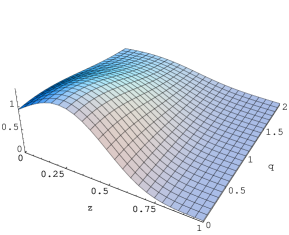
Figure 7.1: Probability distribution $\Phi^{I}(z,\mathbf{q}_{\perp})$ that three valence quarks leave the fraction $z$ of the baryon momentum and transverse momentum $\mathbf{q}_{\perp}$ to the quark-antiquark pair(s) in the axial $I=A$ (left) and tensor $I=T$ (right) cases plotted in units of $M$ and normalized to $\Phi^{V}(0,0)=1$.

While in the non-relativistic limit valence probability distributions are the same, relativistic corrections (quark angular momentum) are different in axial and tensor cases. This is of course due to the difference in structure between (6.8) and (7.12).

In the following we give the integrals appearing in each Fock sector and the numerical values obtained for them. In the evaluation of the scalar overlap integrals we have used the constituent quark mass $M=345$ MeV, the Pauli-Villars mass $M_{\textrm{PV}}=556.8$ MeV for the regularization of (3.61)-(3.65) and the baryon mass $\mathcal{M}=1207$ MeV as it follows for the “classical” mass in the mean field approximation [114].

7.3.1 $3Q$ scalar integral

In the $3Q$ sector there is no quark-antiquark pair and thus only one integral is involved. It corresponds to the valence quark distribution without momentum left to the sea $\Phi^{T}(0,0)$. We remind that the normalization chosen for $h(p)$ and $j(p)$ is such that $\Phi^{V}(0,0)=1$. From Figure 7.1 one can see that $\Phi^{A}(0,0)<\Phi^{T}(0,0)<1$. The precise value is

$$\Phi^{T}(0,0)=0.93058.$$ (7.15)

This means that in a simple $3Q$ picture all NQM tensor charges have to be multiplied by this factor. Not surprisingly this is the same prescription as the one encountered in a standard light-cone approach based on Melosh rotation. Valence quark motion is a relativistic effect and is responsible for a noticeable reduction of NQM predictions. The Melosh reduction factor 7/8 is of course smaller than the one we have obtained because of the function $h(p)$ absent in the Melosh approach but necessary in a fully relativistic treatment. Since we know analytically that the pure $3Q$ contribution saturates Soffer’s inequality one can notice that the numerical accuracy of the distributions is good.

The NQM is recovered in the $3Q$ non-relativistic limit only, i.e. where the three valence quarks have no orbital angular momentum and thus $\Phi^{T}_{NR}(0,0)=\Phi^{A}_{NR}(0,0)=\Phi^{V}_{NR}(0,0)=1$.

7.3.2 $5Q$ scalar integrals

In the $5Q$ sector there is one quark-antiquark pair. Contractions given by the direct diagram give three different integrals $J=\pi\pi,33,\sigma\sigma$. If the tensor operator acts on valence quarks, the quark-antiquark pair is not affected and thus the integrals present the vector structure for the sea. If the tensor operator acts on the sea, the valence quarks are not affected and the vector valence probability distribution has to be used. However no structure for the sea survives in this case. The integrals are identically zero. This is due to the fact that the tensor operator is chiral odd. Since the tensor operator flips one quark spin it would transform a quark-antiquark pair with zero total angular momentum into another one with one unit of angular momentum, which is not allowed in the model. This means that only valence quarks contribute to tensor charges, in accordance with the usual definition of valence quarks. Note however that the usual definition of valence quarks forbids strange quark contribution to tensor charge while with our definition strangeness can access to the valence sector thanks to the $5Q$ component.

Here are the numerical values obtained for the three new integrals

$$K^{T}_{\pi\pi}=0.03328,\qquad K^{T}_{33}=0.01802,\qquad K^{T}_{\sigma\sigma}=0.01261.$$ (7.16)

Let us have a look to the ratios $K^{T}_{J}/K^{V}_{J}$ with $J=\pi\pi,33,\sigma\sigma$

$$\frac{K^{T}_{\pi\pi}}{K^{V}_{\pi\pi}}=0.91114,\qquad\frac{K^{T}_{33}}{K^{V}_{33}}=0.91229,\qquad\frac{K^{T}_{\sigma\sigma}}{K^{V}_{\sigma\sigma}}=0.90020.$$ (7.17)

The reduction is of the same order as in the $3Q$ sector. It is however different from one structure to another due to the details of the valence probability distributions.

7.4 Combinatoric Results

Tensor matrix elements are linear combinations of the tensor scalar overlap integrals. These specific combinations are obtained by contracting the baryon rotational wave functions with the tensor operator. In the following we give for each multiplet the combinations obtained. We remind that for tensor charges valence quark only contribute.

7.4.1 Octet baryons

In the $3Q$ sector we have obtained

$$\alpha_{T,q_{\textrm{val}}}^{(3)}=12\Phi^{T}(0,0),\qquad\beta_{T,q_{\textrm{val}}}^{(3)}=-3\Phi^{T}(0,0),\qquad\gamma_{T,q_{\textrm{val}}}^{(3)}=0.$$ (7.18)

These factors are not surprising since in the non-relativistic limit $\Phi^{T}_{NR}(0,0)=\Phi^{A}_{NR}(0,0)$ we have to recover $\Delta q_{NR}=\delta q_{NR}$.

In the $5Q$ sector the combinations are

$$\alpha_{T,q_{\textrm{val}}}^{(5)}=\frac{6}{5}\left(30K^{T}_{\pi\pi}-K^{T}_{33}+91K^{T}_{\sigma\sigma}\right),$$ (7.19)

$$\beta_{T,q_{\textrm{val}}}^{(5)}=\frac{-12}{25}\left(21K^{T}_{\pi\pi}+11K^{T}_{33}+52K^{T}_{\sigma\sigma}\right),$$ (7.20)

$$\gamma_{T,q_{\textrm{val}}}^{(5)}=\frac{-12}{25}\left(3K^{T}_{\pi\pi}+8K^{T}_{33}+K^{T}_{\sigma\sigma}\right).$$ (7.21)

The first observation is that global factors are the same as in the axial case and that the factors in front of $K_{\sigma\sigma}$ correspond. If one looks closer one can notice that the differences are always proportional to the structure $K_{\pi\pi}-3K_{33}$. This means that tensor charges together with axial charges, besides giving informations on quark spin distribution, valence quarks number and motion, might give also informations on quadrupolar distortion of the baryon shape.

7.4.2 Decuplet baryons

In the $3Q$ sector we have obtained

$$\alpha^{\prime(3)}_{T,q_{\textrm{val}},3/2}=3\alpha^{\prime(3)}_{T,q_{\textrm{val}},1/2}=\frac{18}{5}\,\Phi^{T}(0,0),\qquad\beta^{\prime(3)}_{T,q_{\textrm{val}},3/2}=3\beta^{\prime(3)}_{T,q_{\textrm{val}},1/2}=0.$$ (7.22)

In the $5Q$ sector the combinations are

$$\alpha^{\prime(5)}_{T,q_{\textrm{val}},3/2}=\frac{9}{20}\left(40K^{T}_{\pi\pi}-7K^{T}_{33}+67K^{T}_{\sigma\sigma}\right),$$ (7.23)

$$\alpha^{\prime(5)}_{T,q_{\textrm{val}},1/2}=\frac{3}{20}\left(30K^{T}_{\pi\pi}+23K^{T}_{33}+67K^{T}_{\sigma\sigma}\right),$$ (7.24)

$$\beta^{\prime(5)}_{T,q_{\textrm{val}},3/2}=\frac{-9}{20}\left(8K^{T}_{\pi\pi}+13K^{T}_{33}-K^{T}_{\sigma\sigma}\right),$$ (7.25)

$$\beta^{\prime(5)}_{T,q_{\textrm{val}},1/2}=\frac{-3}{20}\left(6K^{T}_{\pi\pi}+19K^{T}_{33}-K^{T}_{\sigma\sigma}\right).$$ (7.26)

If the decuplet baryon was made of three quarks only then one would have the following relations between spin-3/2 and 1/2 tensor contributions

$$T_{3/2}=3T_{1/2}.$$ (7.27)

This picture presents the $\Delta$ as a spherical particle. Things change in the $5Q$ sector. One notices directly that the relation is broken by a unique structure $(K^{T}_{\pi\pi}-3K^{T}_{33})$. We can draw the same conclusion as in the axial and vector cases. The pion field is directly responsible for the deviation of decuplet baryon from spherical shape. Moreover this structure is the only difference between axial and tensor combinations. This supports further what we have observed with octet baryons.

7.4.3 Antidecuplet baryons

In the $5Q$ sector one has

$$\alpha^{\prime\prime(5)}_{T,q_{\textrm{val}}}=\beta^{\prime\prime(5)}_{T,q_{\textrm{val}}}=\frac{-6}{5}\left(K^{T}_{33}-K^{T}_{\sigma\sigma}\right).$$ (7.28)

In the $5Q$ sector of $\Theta^{+}$ pentaquark the strange flavor appears only as an antiquark as one can see from its minimal quark content $uudd\bar{s}$. That’s the reason why we have found no strange contribution. But if at least the $7Q$ sector was considered we would have obtained a nonzero contribution due to flavor components like $|uus(d\bar{s})(d\bar{s})\rangle$, $|uds(u\bar{s})(d\bar{s})\rangle$ and $|dds(u\bar{s})(u\bar{s})\rangle$.

Even for exotic baryons the only difference between tensor and axial combinations is proportional to the quadrupolar structure $K_{\pi\pi}-3K_{33}$ of the pion cloud.

7.5 Numerical results and discussion

7.5.1 Octet content

We give in Table 7.1 the values obtained for the proton tensor charges at the model scale $Q_{0}^{2}=0.36$ GeV².

Table 7.1: Our proton tensor charges computed at the model scale $Q_{0}^{2}=0.36$ GeV².

$p^{+}$	$\delta u$	$\delta d$	$\delta s$	$g_{T}^{(3)}$	$g_{T}^{(8)}$	$g_{T}^{(0)}$
$3Q$	1.241	-0.310	0	1.551	0.537	0.931
$3Q+5Q$	1.172	-0.315	-0.011	1.487	0.507	0.846

Many papers are just concerned with the isovector (3) and isoscalar (0) combinations. They assume that strangeness appears only in the sea or even forget completely about proton strangeness. We have shown however that the $5Q$ component introduces strangeness in the valence sector and gives the possibility to have non-zero strange contribution to tensor charges. This strange contribution is negative while it was positive in the axial sector. In fact only the valence contributions should be compared. In the axial case the strange valence contribution is also negative. The sea was positive and larger in magnitude.

Like all other models for the proton $\delta u$ and $\delta d$ are not small and have a magnitude similar to $\Delta u$ and $\Delta d$. One can also check that Soffer’s inequality (7.5) is satisfied for explicit flavors. However the hidden flavor, i.e. $s$ in proton, violates the inequality.

Up to now only one experimental extraction of transversity distributions has been achieved [171]. The authors did not give explicit values for tensor charges. They have however been estimated to $\delta u=0.46^{+0.36}_{-0.28}$ and $\delta d=-0.19^{+0.30}_{-0.23}$ in [167] at the scale $Q^{2}=0.4$ GeV². These values are unexpectedly small compared to models predictions. Further experimental results are then highly desired to either confirm or infirm the smallness of tensor charges. If it is confirmed then it will be very difficult to explain this within a quark model while keeping rather large values for the axial charges. The question is of course very intriguing and might eventually kill a constituent quark approach.

7.5.2 Decuplet content

We give in Table 7.2 the values obtained for the $\Delta^{++}$ tensor charges at the model scale $Q_{0}^{2}=0.36$ GeV².

Table 7.2: Our $\Delta^{++}$ tensor charges computed at the model scale $Q_{0}^{2}=0.36$ GeV².

$\Delta^{++}_{3/2}$	$\delta u$	$\delta d$	$\delta s$	$g_{T}^{(3)}$	$g_{T}^{(8)}$	$g_{T}^{(0)}$
$3Q$	2.792	0	0	2.792	1.612	2.792
$3Q+5Q$	2.624	-0.046	-0.046	2.670	1.541	2.532
$\Delta^{++}_{1/2}$	$\delta u$	$\delta d$	$\delta s$	$g_{T}^{(3)}$	$g_{T}^{(8)}$	$g_{T}^{(0)}$
$3Q$	0.931	0	0	0.931	0.537	0.931
$3Q+5Q$	0.863	-0.016	-0.016	0.879	0.508	0.831

Like in the proton one can see that hidden flavors, i.e. $d$ and $s$ for $\Delta^{++}$, violate Soffer’s inequality. There is no experimental data concerning decuplet baryon tensor charges. Our results are then just predictions.

7.5.3 Antidecuplet content

We give in Table 7.3 the values obtained for the $\Theta^{+}$ tensor charges at the model scale $Q_{0}^{2}=0.36$ GeV².

Table 7.3: Our $\Theta^{+}$ tensor charges computed at the model scale $Q_{0}^{2}=0.36$ GeV².

$\Theta^{+}$	$\delta u$	$\delta d$	$\delta s$	$g_{T}^{(3)}$	$g_{T}^{(8)}$	$g_{T}^{(0)}$
$5Q$	-0.053	-0.053	0	0	-0.062	-0.107

The vanishing value of the strange contribution is of course due to the truncation at the $5Q$ sector. The $7Q$ component is the main cause for the presence of strange quarks in the valence sector and consequently in $\Theta^{+}$ pentaquark tensor charges.

Chapter 8 Magnetic and transition magnetic moments

8.1 Introduction

The study of electromagnetic properties of the nucleon is of great importance in understanding the structure of baryons (see reviews [172]). Indeed, since electrons are point-like particles, any observed structure in the electron-target collisions directly gives information on the target structure. This information is encoded within form factors which have been measured more and more accurately throughout the last decades. Form factors measurement revealed the role of quark orbital momentum, scale at which perturbative QCD effects should become evident, strangeness content of the proton and meson-cloud effects. For more than ten years the contribution of $s$-quarks to proton electric and magnetic form factors [42, 43, 44, 45] has focused interests because this contribution is believed to come from the quark-antiquark sea (meson cloud). There is no more doubt that both valence and sea-quark effects are important in the description of electromagnetic properties of light hadrons. The only question left now is the amplitude of this meson-cloud contribution.

We split the contribution to the moments into valence quark, sea quark and antiquark contributions

$$G_{M,E,q}=G_{M,E,q_{\textrm{val}}}+G_{M,E,q_{\textrm{sea}}},\qquad G_{M,E,q_{\textrm{sea}}}=G_{M,E,q_{\textrm{s}}}-G_{M,E,\bar{q}}$$ (8.1)

where index s refers to the quarks in the sea pairs.

From the NQM picture one could think that magnetic moments could be related to the axial content of the proton because they are proportional to the longitudinal polarization asymmetry $\Delta q$. Actually this is not the case because of the antiquark contribution has a different sign: axial charges are in flavor singlet combination (quarks plus antiquarks) $A\sim\Delta q+\Delta\bar{q}$ and magnetic moments in flavor non-singlet combination (quarks minus antiquarks) $M\sim\Delta q-\Delta\bar{q}$.

8.2 Magnetic and transition magnetic moments on the light cone

We consider in this study the interaction of an electromagnetic field with baryons at the quark level. Constituent quarks can be considered as quasiparticles. Their coupling with a photon is then modulated by form factors $F_{1}^{q}$, $F_{2}^{q}$ that encode in an effective way the other degrees of freedom, e.g. gluons and quark-antiquark pairs. In the present approach the gluon field has been integrated out leaving as a by-product an effective pion mean field that binds quarks together. The model gives a description of the three valence quark and of the whole Dirac sea. Baryons appear naturally as made of three quarks plus a certain number of quark-antiquark pairs. Since this degree of freedom is explicitly taken into account, we consider constituent quarks as point-like particles. This means that the Dirac form factor is just the quark charge $F_{1}^{q}=Q$ and the Pauli form factor is identically zero $F_{2}^{q}=0$. The whole anomalous baryon magnetic moments then come from quark orbital moment and quark-antiquark pairs.

Baryon form factors are obtained through computation of some matrix elements of the electromagnetic current. We have used the following vector current $J_{\mu}(0)=\bar{q}Q_{q}\gamma_{\mu}q$ where $q$ is a set of three free Dirac spinor of definite flavor $q=u,d,s$ and $Q_{q}$ is the quark charge matrix diag$=(2/3,-1/3,-1/3)$. Since we are only concerned so far with magnetic moments, form factors are computed only for $Q^{2}=-q^{2}=0$ (real photon) where $q=p^{\prime}-p$ is the momentum transfer, $p^{\prime}$ and $p$ are respectively the momenta of outgoing and incoming baryon.

We give below explicit definitions of form factors and recall how to extract them when the system is described in the IMF.

8.2.1 Octet form factors

Octet baryons are spin-$\frac{1}{2}$ particles. Their interaction with an electromagnetic field involves two form factors known as Dirac and Pauli form factors

$$\langle B(p^{\prime},s^{\prime})|J^{\mu}|B(p,s)\rangle=\bar{u}_{B}(p^{\prime},s^{\prime})\left[\gamma^{\mu}F_{1}(q^{2})+i\frac{\sigma^{\mu\nu}q_{\nu}}{2M_{B}}F_{2}(q^{2})\right]u_{B}(p,s)$$ (8.2)

where $s$ and $s^{\prime}$ are the component of the spin along $z$ axis. At zero momentum transfer $F_{1}(0)$ and $F_{2}(0)$ correspond respectively to the charge and anomalous magnetic moment of the baryon. In the literature one also often defines another set of form factors known as Sachs form factors [173] that are combinations of the previous ones

$$G_{E}(Q^{2})=F_{1}(Q^{2})-\frac{Q^{2}}{4M_{B}^{2}}F_{2}(Q^{2}),\qquad G_{M}(Q^{2})=F_{1}(Q^{2})+F_{2}(Q^{2})$$ (8.3)

which express the nucleon electric and magnetic form factors. In the Breit frame and in the non-relativistic limit, their three-dimensional Fourier transforms give electric-charge-density distribution and magnetic-current-density distribution within the baryon [174]. At zero momentum transfer $-q^{2}=Q^{2}=0$ one obtains naturally $G_{E}(0)=F_{1}(0)=Q_{B}$ where $Q_{B}$ is the baryon charge and $G_{M}(0)=G_{E}(0)+\kappa=F_{1}(0)+F_{2}(0)=\mu_{B}$ where $\mu_{B}$ is the baryon magnetic moment and $\kappa=F_{2}(0)$ is the anomalous baryon magnetic moment expressed in units of $e/2M_{B}$.

These form factors can be extracted in the IMF from the spin-conserving and spin-flip matrix elements of the + component of the electromagnetic current

$$F_{1}(0) = \langle P,\frac{1}{2}|\frac{J^{+}(0)}{2P^{+}}|P,\frac{1}{2}\rangle,$$ (8.4)

$$-q_{L}F_{2}(Q^{2}) = 2M_{B}\langle P,\frac{1}{2}|\frac{J^{+}(0)}{2P^{+}}|P,-\frac{1}{2}\rangle$$ (8.5)

with $q_{L}=q_{1}-iq_{2}$. It is convenient to work in the DYW frame ($q^{+}=0$ [98, 110]) where the photon momentum is transverse to incident baryon momentum (chosen to be directed along the $z$ direction)

$$P^{\mu}=\left(P^{+},\mathbf{0}_{\perp},\frac{M_{B}^{2}}{P^{+}}\right),\qquad q^{\mu}=\left(0,\mathbf{q}_{\perp},\frac{2q\cdot P}{P^{+}}\right).$$ (8.6)

This prevents the quark current $J^{+}$ from creating pairs or annihilating the vacuum. One also has $-q_{\mu}q^{\mu}\equiv Q^{2}=\mathbf{q}_{\perp}^{2}$. The Pauli form factor of nucleons is therefore computed from the overlap of light-cone wave functions differing by one unit of orbital angular momentum $\Delta L_{z}=\pm 1$. The fact that anomalous magnetic moment of the proton is not zero is an immediate signal for the presence of non-zero angular momentum in the proton wave function [175].

8.2.2 Decuplet form factors

Decuplet baryons are spin-3/2 particles. Their interaction with an electromagnetic field involves four multipoles: a coulomb monopole (C0), a magnetic dipole (M1), an electric quadrupole (E2) and a magnetic octupole (M3). One has

$$\langle B(p^{\prime},s^{\prime})|J^{\mu}|B(p,s)\rangle=\bar{u}_{B\alpha}(p^{\prime},s^{\prime})\mathcal{O}^{\alpha\beta\mu}u_{B\beta}(p,s)$$ (8.7)

where $u_{B\beta}(p,s)$ is a Rarita-Schwinger spin vector [176] with the subsidiary conditions $\gamma^{\mu}u_{\mu}(p,s)=p^{\mu}u_{\mu}(p,s)=0$. The tensor has the following Lorentz-covariant form

$$\mathcal{O}^{\alpha\beta\mu}=g^{\alpha\beta}\left[\gamma^{\mu}F_{1}(q^{2})+i\frac{\sigma^{\mu\nu}q_{\nu}}{2M_{B}}F_{2}(q^{2})\right]+\frac{q^{\alpha}q^{\beta}}{(2M_{B})^{2}}\left[\gamma^{\mu}F_{3}(q^{2})+i\frac{\sigma^{\mu\nu}q_{\nu}}{2M_{B}}F_{4}(q^{2})\right].$$ (8.8)

This set of form factors is related to the multipole form factors as follows when $q^{2}=0$

$$Q_{B} = e\,G_{C0}(0)=e\,F_{1}(0)$$ (8.9)

$$\mu_{B} = \frac{e}{2M_{B}}G_{M1}(0)=\frac{e}{2M_{B}}\left[F_{1}(0)+F_{2}(0)\right]$$ (8.10)

$$\mathcal{Q}_{B} = \frac{e}{M_{B}^{2}}G_{E2}(0)=\frac{e}{M_{B}^{2}}\left[F_{1}(0)-\frac{1}{2}F_{3}(0)\right]$$ (8.11)

$$O_{B} = \frac{e}{2M_{B}^{3}}G_{M3}(0)=\frac{e}{2M_{B}^{3}}\left\{F_{1}(0)+F_{2}(0)-\frac{1}{2}\left[F_{3}(0)+F_{4}(0)\right]\right\}.$$ (8.12)

In this paper, we are only interested in $F_{1}(0)$ and $F_{2}(0)$ form factors, i.e. charge and anomalous magnetic moment respectively. These can be extracted in the IMF from the matrix elements of the + component of the electromagnetic current [177]

$$F_{1}(0) = \langle P,\frac{3}{2}|\frac{J^{+}(0)}{2P^{+}}|P,\frac{3}{2}\rangle,$$ (8.13)

$$-q_{L}F_{2}(0) = 2\left[\sqrt{3}M_{B}\langle P,\frac{3}{2}|\frac{J^{+}(0)}{2P^{+}}|P,\frac{1}{2}\rangle-q_{L}\langle P,\frac{3}{2}|\frac{J^{+}(0)}{2P^{+}}|P,\frac{3}{2}\rangle\right].$$ (8.14)

8.2.3 Octet-to-decuplet form factors

Imposing Lorentz covariance, gauge invariance and parity conservation, the matrix element of the vector octet-to-decuplet transition can be parametrized in terms of three form factors only [178]

$$\langle B_{\bf 10}(p^{\prime},s^{\prime})|J^{\mu}|B_{\bf 8}(p,s)\rangle=\sqrt{\frac{2}{3}}\bar{u}_{B_{\bf 10}\alpha}(p^{\prime},s^{\prime})\mathcal{O}^{\alpha\mu}\gamma_{5}u_{B_{\bf 8}}(p,s)$$ (8.15)

where $\sqrt{2/3}$ is the isospin factor and

$$\mathcal{O}^{\alpha\mu}=(q^{\alpha}\gamma^{\mu}-g^{\alpha\mu}q\!\!\!/)G_{1}(q^{2})+(q^{\alpha}P^{\mu}-g^{\alpha\mu}P\cdot q)G_{2}(q^{2})+(q^{\alpha}q^{\mu}-g^{\alpha\mu}q^{2})G_{3}(q^{2})$$ (8.16)

with $P=(p+p^{\prime})/2$. Since in our case the photon is real, $G_{3}$ does not contribute and only the form factors $G_{1}$ and $G_{2}$ are needed. These form factors are related to multipole (Jones-Scadron [178]) ones as follows

$$G^{*}_{M} = \frac{m_{\mathcal{O}}}{3}\left[(3M_{\mathcal{D}}+m_{\mathcal{O}})\frac{G_{1}}{M_{\mathcal{D}}}+(M_{\mathcal{D}}-m_{\mathcal{O}})G_{2}\right],$$ (8.17)

$$G^{*}_{E} = \frac{m_{\mathcal{O}}(M_{\mathcal{D}}-m_{\mathcal{O}})}{3}\left[\frac{G_{1}}{M_{\mathcal{D}}}+G_{2}\right]$$ (8.18)

where $M_{\mathcal{D}}$ is the decuplet and $m_{\mathcal{O}}$ the octet baryon mass. In the literature one also defines helicity amplitudes

$$A_{M}=-e\frac{1}{\sqrt{2\omega}}\langle B_{\bf 10},M|\vec{j}\cdot\vec{\epsilon}|B_{\bf 8},M-1\rangle,\qquad M=\frac{1}{2},\frac{3}{2}$$ (8.19)

where $\omega=(M_{\mathcal{D}}^{2}-m_{\mathcal{O}}^{2})/2M_{\mathcal{D}}$ is the energy of the photon in the rest frame of decuplet baryon with polarization $\vec{\epsilon}$. These amplitudes can be expressed in terms of magnetic dipole $M1$ and electric quadrupole $E2$ moments

$$A_{3/2}=-\frac{\sqrt{3}}{2}(M1-E2),\qquad A_{1/2}=-\frac{1}{2}(M1+3E2)$$ (8.20)

which are related to multipole form factors as follows

$$M1=\frac{e}{2m_{\mathcal{O}}}\sqrt{\frac{M_{\mathcal{D}}\omega}{m_{\mathcal{O}}}}G^{*}_{M},\qquad E2=-\frac{e}{2m_{\mathcal{O}}}\sqrt{\frac{M_{\mathcal{D}}\omega}{m_{\mathcal{O}}}}G^{*}_{E}.$$ (8.21)

The static transition magnetic moment $\mu_{B_{\bf 8}B_{\bf 10}}$ is obtained from magnetic dipole form factor $G^{*}_{M}$ at $Q^{2}=0$ by

$$\mu_{B_{\bf 8}B_{\bf 10}}=\sqrt{\frac{M_{\mathcal{D}}}{m_{\mathcal{O}}}}G^{*}_{M}(0)$$ (8.22)

which can be expressed in nuclear magnetons $\mu_{N}\equiv e/2M_{N}$ if one adds the factor $M_{N}/m_{\mathcal{O}}$ to the rhs.

The static transition quadrupole moment $\mathcal{Q}_{B_{\bf 8}B_{\bf 10}}$ is related to the electric quadrupole form factor $G^{*}_{E}$ at $Q^{2}=0$ by

$$\mathcal{Q}_{B_{\bf 8}B_{\bf 10}}=-6\sqrt{\frac{M_{\mathcal{D}}}{m_{\mathcal{O}}}}\frac{1}{m_{\mathcal{O}}\omega}G^{*}_{E}(0)$$ (8.23)

There is a special interest in the multipole ratio which directly indicates a deviation from spherical symmetry

$$R_{EM}\equiv\frac{E2}{M1}=-\frac{G^{*}_{E}}{G^{*}_{M}}=\frac{A_{1/2}-A_{3/2}/\sqrt{3}}{A_{1/2}+\sqrt{3}A_{3/2}}.$$ (8.24)

The electromagnetic width is given by the formula

$$\Gamma_{B_{\bf 10}B_{\bf 8}}=\frac{\omega^{2}}{2\pi}\frac{m_{\mathcal{O}}}{M_{\mathcal{D}}}\left\{|A_{3/2}|^{2}+|A_{1/2}|^{2}\right\}=\frac{\omega^{2}}{2\pi}\frac{m_{\mathcal{O}}}{M_{\mathcal{D}}}\left\{|M1|^{2}+3|E2|^{2}\right\}=\frac{\omega^{3}\alpha}{2m_{\mathcal{O}}^{2}}\left\{G_{M}^{*2}+3G_{E}^{*2}\right\}$$ (8.25)

where $\alpha=e^{2}/4\pi=1/137$.

In the IMF, one can extract $G_{1}(0)$ and $G_{2}(0)$ from the following matrix elements [179]

$$I_{\frac{3}{2},\frac{1}{2}}\equiv\langle P,\frac{3}{2}|\frac{J^{+}(0)}{2P^{+}}|P,\frac{1}{2}\rangle = \frac{q_{L}}{\sqrt{3}}\left[G_{1}+\frac{M_{\mathcal{D}}-m_{\mathcal{O}}}{2}G_{2}\right],$$ (8.26)

$$I_{\frac{1}{2},-\frac{1}{2}}\equiv\langle P,\frac{1}{2}|\frac{J^{+}(0)}{2P^{+}}|P,-\frac{1}{2}\rangle = -\frac{q_{L}}{3}\left[-\frac{m_{\mathcal{O}}}{M_{\mathcal{D}}}G_{1}+\frac{M_{\mathcal{D}}-m_{\mathcal{O}}}{2}G_{2}\right].$$ (8.27)

8.3 Scalar overlap integrals and quark distributions

From the expression (3.35) and if we concentrate on the spin part the contraction of two valence wave functions $F$ gives when the baryon helicity is flipped

$$F^{\dagger}F\propto h(p)\frac{1}{|\mathbf{p}|}j(p)+\frac{p_{z}}{p^{2}}j^{2}(p).$$ (8.28)

The physical interpretation is straightforward. The magnetic operator conserves the struck quark helicity but the total baryon spin is flipped. The quark absorbs one unit of angular momentum and thus jumps from a $L_{z}=0$ state to a $L_{z}\neq 0$ state. This unit of angular momentum comes from the photon.

The magnetic valence quark distribution is obtained by the multiplication of two factors with structure (5.10) where the momentum is respectively $p_{1}$ and $p_{2}$ and a third factor with structure (8.28) and momentum $p_{3}$. The expansion gives the following function $D$

$$D^{M}(p_{1},p_{2},p_{3})=h^{2}(p_{1})h^{2}(p_{2})\left[h(p_{3})\frac{1}{|\mathbf{p}_{3}|}j(p_{3})\right]+h^{2}(p_{1})h^{2}(p_{2})\frac{p_{3z}}{p_{3}^{2}}j^{2}(p_{3})$$

$$+4h^{2}(p_{1})\left[h(p_{2})\frac{p_{2z}}{|\mathbf{p}_{2}|}j(p_{2})\right]\left[h(p_{3})\frac{1}{|\mathbf{p}_{3}|}j(p_{3})\right]+2h^{2}(p_{1})j^{2}(p_{2})\left[h(p_{3})\frac{1}{|\mathbf{p}_{3}|}j(p_{3})\right]$$

$$+4h^{2}(p_{1})\left[h(p_{2})\frac{p_{2z}}{|\mathbf{p}_{2}|}j(p_{2})\right]\frac{p_{3z}}{p_{3}^{2}}j^{2}(p_{3})+4\left[h(p_{1})\frac{p_{1z}}{|\mathbf{p}_{1}|}j(p_{1})\right]\left[h(p_{2})\frac{p_{2z}}{|\mathbf{p}_{2}|}j(p_{2})\right]\left[h(p_{3})\frac{1}{|\mathbf{p}_{3}|}j(p_{3})\right]$$ (8.29)

$$+2h^{2}(p_{1})j^{2}(p_{2})\frac{p_{3z}}{p_{3}^{2}}j^{2}(p_{3})+4\left[h(p_{1})\frac{p_{1z}}{|\mathbf{p}_{1}|}j(p_{1})\right]j^{2}(p_{2})\left[h(p_{3})\frac{1}{|\mathbf{p}_{3}|}j(p_{3})\right]$$

$$+4\left[h(p_{1})\frac{p_{1z}}{|\mathbf{p}_{1}|}j(p_{1})\right]\left[h(p_{2})\frac{p_{2z}}{|\mathbf{p}_{2}|}j(p_{2})\right]\frac{p_{3z}}{p_{3}^{2}}j^{2}(p_{3})+j^{2}(p_{1})j^{2}(p_{2})\left[h(p_{3})\frac{1}{|\mathbf{p}_{3}|}j(p_{3})\right]$$

$$+4\left[h(p_{1})\frac{p_{1z}}{|\mathbf{p}_{1}|}j(p_{1})\right]j^{2}(p_{2})\frac{p_{3z}}{p_{3}^{2}}j^{2}(p_{3})+j^{2}(p_{1})j^{2}(p_{2})\frac{p_{3z}}{p_{3}^{2}}j^{2}(p_{3}).$$

that is needed in the expression of the valence quark distribution (3.59). In the non-relativistic limit $j=0$ this function $D$ is identically zero. Magnetic moment is a purely relativistic property on the light cone. Relativistic corrections (quark angular momentum) are clearly essential to compute baryon magnetic and transition magnetic moments.

The magnetic valence probability distribution $\Phi^{M}(z,\mathbf{q}_{\perp})$ is then obtained by integration over the valence quark momenta, see eq. (3.59) and is depicted in Fig. 8.1 in vector $I=V$ and magnetic $I=M$ cases.

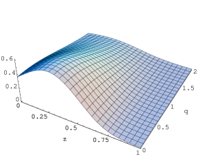
Figure 8.1: Probability distribution $\Phi^{I}(z,\mathbf{q}_{\perp})$ that three valence quarks leave the fraction $z$ of the baryon momentum and transverse momentum $\mathbf{q}_{\perp}$ to the quark-antiquark pair(s) in the vector $I=V$ (left) and magnetic $I=M$ (right) cases plotted in units of $M$ and normalized to $\Phi^{V}(0,0)=1$.

In the following we give the integrals appearing in each Fock sector and the numerical values obtained for them. In the evaluation of the scalar overlap integrals we have used the constituent quark mass $M=345$ MeV, the Pauli-Villars mass $M_{\textrm{PV}}=556.8$ MeV for the regularization of (3.61)-(3.65) and the baryon mass $\mathcal{M}=1207$ MeV as it follows for the “classical” mass in the mean field approximation [114].

8.3.1 $3Q$ scalar integral

In the $3Q$ sector there is no quark-antiquark pair and thus only one integral is involved. It corresponds to the valence quark distribution without momentum left to the sea $\Phi^{M}(0,0)$. Its precise value is

$$\Phi^{M}(0,0)=0.36210.$$ (8.30)

In the non-relativistic limit $j=0$ it is zero. The extraction of magnetic moment from spin-flip matrix elements is essentially a relativistic procedure since it implies quarks to have orbital angular momentum. In the usual light-cone approach this quark orbital motion is introduced by the Melosh rotation.

8.3.2 $5Q$ scalar integrals

In the $5Q$ sector there is one quark-antiquark pair. Contractions given by the direct diagram give four different integrals $J=\pi\pi,33,\sigma\sigma,332$. If the magnetic operator acts on valence quarks, the quark-antiquark pair is not affected and thus the integrals present the vector structure for the sea. If the magnetic operator acts on the sea, the valence quark are not affected and the vector valence probability distribution has to be used. The integrals present a new structure for the sea. Here the quark-antiquark pair cannot use the unit of orbital angularmomentum in its internal motion but can use it in its orbital motion.

Here are the numerical values obtained for the four new integrals

$$K^{M}_{\pi\pi}=0.01445,\qquad K^{M}_{33}=0.00799,\qquad K^{M}_{\sigma\sigma}=0.00566,\qquad K^{V}_{332}=0.03542.$$ (8.31)

Let us have a look to the ratios $K^{M}_{J}/K^{V}_{J}$ with $J=\pi\pi,33,\sigma\sigma$

$$\frac{K^{M}_{\pi\pi}}{K^{V}_{\pi\pi}}=0.39559,\qquad\frac{K^{M}_{33}}{K^{V}_{33}}=0.40482,\qquad\frac{K^{M}_{\sigma\sigma}}{K^{V}_{\sigma\sigma}}=0.40420.$$ (8.32)

The reduction is of the same order as in the $3Q$ sector. It is however different from one structure to another due to the details of the valence probability distributions. Note also that contrarily to axial and tensor cases, the reduction factor is larger in the $5Q$ sector than in the $3Q$ sector.

8.4 Combinatoric Results

8.4.1 Octet baryons

In the $3Q$ sector there is no quark-antiquark pair and thus only valence quarks contribute to magnetic moments

$$\alpha_{M,q_{\textrm{val}}}^{(3)}=12\,\Phi^{M}(0,0)\,2\mathcal{M},\qquad\beta_{M,q_{\textrm{val}}}^{(3)}=-3\,\Phi^{M}(0,0)\,2\mathcal{M},\qquad\gamma_{M,q_{\textrm{val}}}^{(3)}=0.$$ (8.33)

as it is expected from NQM. In the $5Q$ sector one has

$$\alpha_{M,q_{\textrm{val}}}^{(5)}=\frac{6}{5}\left(30K^{M}_{\pi\pi}-K^{M}_{33}+91K^{M}_{\sigma\sigma}\right)\,2\mathcal{M},\quad\alpha_{M,q_{\textrm{s}}}^{(5)}=\frac{-96}{5}\,K^{V}_{332}\,2\mathcal{M},\quad\alpha_{M,\bar{q}}^{(5)}=-6\,K^{V}_{332}\,2\mathcal{M},$$ (8.34)

$$\beta_{M,q_{\textrm{val}}}^{(5)}=\frac{-12}{25}\left(21K^{M}_{\pi\pi}+11K^{M}_{33}+52K^{M}_{\sigma\sigma}\right)\,2\mathcal{M},\quad\beta_{M,q_{\textrm{s}}}^{(5)}=\frac{-48}{25}\,K^{V}_{332}\,2\mathcal{M},\quad\beta_{M,\bar{q}}^{(5)}=6\,K^{V}_{332}\,2\mathcal{M},$$ (8.35)

$$\gamma_{M,q_{\textrm{val}}}^{(5)}=\frac{-12}{25}\left(3K^{M}_{\pi\pi}+8K^{M}_{33}+K^{M}_{\sigma\sigma}\right)\,2\mathcal{M},\quad\gamma_{M,q_{\textrm{s}}}^{(5)}=\frac{6}{25}\,K^{V}_{332}\,2\mathcal{M},\quad\gamma_{M,\bar{q}}^{(5)}=6\,K^{V}_{332}\,2\mathcal{M}.$$ (8.36)

Notice that the valence combinations are exactly the same as the tensor ones. This is not a coincidence. In both cases one has to compute spin-flip matrix elements. In the tensor case the operator directly flips one valence quark spin while in the magnetic case the valence quark jumps to another orbital state. At the end the result is the same: the total baryon spin has been reversed. The combinations are thus the same and the details concerning the spin-flip are encoded in the integrals.

8.4.2 Decuplet baryons

In the $3Q$ sector there is no quark-antiquark pair and thus only valence quarks contribute to the charges

$$\alpha^{\prime(3)}_{M,q_{\textrm{val}}}=\frac{18}{5}\,\Phi^{M}(0,0)\,2\mathcal{M},\qquad\beta^{\prime(3)}_{M,q_{\textrm{val}}}=0.$$ (8.37)

In the $5Q$ sector one has

$$\alpha^{\prime(5)}_{M,q_{\textrm{val}}}=\frac{9}{20}\left(40K^{M}_{\pi\pi}-7K^{M}_{33}+67K^{M}_{\sigma\sigma}\right)\,2\mathcal{M},\quad\alpha^{\prime(5)}_{M,q_{\textrm{s}}}=\frac{171}{20}\,K^{M}_{332}\,2\mathcal{M},\quad\alpha^{\prime(5)}_{M,\bar{q}}=\frac{-18}{5}\,K^{M}_{332}\,2\mathcal{M},$$ (8.38)

$$\beta^{\prime(5)}_{M,q_{\textrm{val}}}=\frac{-9}{20}\left(8K^{M}_{\pi\pi}+13K^{M}_{33}-K^{M}_{\sigma\sigma}\right)\,2\mathcal{M},\quad\beta^{\prime(5)}_{M,q_{\textrm{s}}}=\frac{9}{20}\,K^{M}_{332}\,2\mathcal{M},\quad\beta^{\prime(5)}_{M,\bar{q}}=\frac{63}{5}\,K^{M}_{332}\,2\mathcal{M}.$$ (8.39)

8.4.3 Antidecuplet baryons

In the $5Q$ sector one has

$$\alpha^{\prime\prime(5)}_{M,q_{\textrm{val}}}=\frac{-6}{5}\left(K^{M}_{33}-K^{M}_{\sigma\sigma}\right)\,2\mathcal{M},\quad\alpha^{\prime\prime(5)}_{M,q_{\textrm{s}}}=\frac{6}{5}\,K^{M}_{332}\,2\mathcal{M},\quad\alpha^{\prime\prime(5)}_{M,\bar{q}}=\frac{-12}{5}\,K^{M}_{332}\,2\mathcal{M},$$ (8.40)

$$\beta^{\prime\prime(5)}_{M,q_{\textrm{val}}}=\frac{-6}{5}\left(K^{M}_{33}-K^{M}_{\sigma\sigma}\right)\,2\mathcal{M},\quad\beta^{\prime\prime(5)}_{M,q_{\textrm{s}}}=\frac{6}{5}\,K^{M}_{332}\,2\mathcal{M},\quad\beta^{\prime\prime(5)}_{M,\bar{q}}=\frac{24}{5}\,K^{M}_{332}\,2\mathcal{M}.$$ (8.41)

8.5 Numerical results and discussion

8.5.1 Octet content

We present in Table 8.1 the results we have obtained for the proton magnetic form factors.

Table 8.1: Our magnetic content of the proton.

Magnetic FF	$G_{M}^{u}$			$G_{M}^{d}$			$G_{M}^{s}$
	$\bar{q}$	$q_{s}$	$q_{val}$	$\bar{q}$	$q_{s}$	$q_{val}$	$\bar{q}$	$q_{s}$	$q_{val}$
$3Q$	0	0	3.378	0	0	-0.845	0	0	0
$3Q+5Q$	0	0.415	3.267	0.256	-0.036	-0.886	0.128	0.005	-0.033

The $5Q$ component naturally introduces a strange contribution to magnetic moments. In this computation it appears that most of strange magnetic moment is due to the strange antiquark. One can see that the $5Q$ component contributes significantly to magnetic moments. Note that we have obtained a negative strange magnetic form factor $G_{M}^{s}(0)=-0.156\,\mu_{N}$ while SAMPLE experiment [42] by measuring the parity-violating asymmetry at backward angles indicated a positive value $G_{M}^{(p)s}(0.1\textrm{(GeV/c)}^{2})=0.37\pm 0.20\pm 0.26\pm 0.07\,\mu_{N}$. This can probably be attributed to the fact that we did not consider flavor $SU(3)$ symmetry breaking . Another possible explanation of our bad strange magnetic moment is the violation of Lorentz covariance due to the impulse approximation (only one-body current and not many-body current is considered) and the truncation of the Fock space [181]. It would not be the case if one includes the complete Fock space [182]. This introduces unphysical form factors which may have a strong impact on the evaluation of the strange magnetic moment and even change its sign [183].

Octet magnetic moments are rather well known. In Table 8.2 we compare our results with experimental values given by the Particle Data Group.

Table 8.2: Our octet magnetic moments compared with experimental data [160].

	$3Q$				$3Q+5Q$
$B$	$G_{M}^{(B)u}$	$G_{M}^{(B)d}$	$G_{M}^{(B)s}$	$\mu_{B}$	$G_{M}^{(B)u}$	$G_{M}^{(B)d}$	$G_{M}^{(B)s}$	$\mu_{B}$	Exp.
$p^{+}_{\mathbf{8}}$	3.378	-0.845	0	2.534	3.683	-1.178	-0.156	2.900	2.793
$n^{0}_{\mathbf{8}}$	-0.845	3.378	0	-1.689	-1.178	3.683	-0.156	-1.961	-1.913
$\Lambda^{0}_{\mathbf{8}}$	0	0	2.534	-0.845	-0.198	-0.198	2.744	-0.981	-$0.613\pm 0.004$
$\Sigma^{+}_{\mathbf{8}}$	3.378	0	-0.845	2.534	3.683	-0.156	-1.178	2.900	$2.458\pm 0.010$
$\Sigma^{0}_{\mathbf{8}}$	1.689	1.689	-0.845	0.845	1.763	1.763	-1.178	0.981	-
$\Sigma^{-}_{\mathbf{8}}$	0	3.378	-0.845	-0.845	-0.156	3.683	-1.178	-0.939	-$1.160\pm 0.025$
$\Xi^{0}_{\mathbf{8}}$	-0.845	0	3.378	-1.689	-1.178	-0.156	3.683	-1.961	-$1.250\pm 0.014$
$\Xi^{-}_{\mathbf{8}}$	0	-0.845	3.378	-0.845	-0.156	-1.178	3.683	-0.939	-$0.651\pm 0.003$
$\Sigma^{0}_{\mathbf{8}}\to\Lambda^{0}_{\mathbf{8}}$	4.388	-4.388	0	1.463	5.095	-5.095	0	1.698	$1.61\pm 0.08$

At the $3Q$ level, all relations specific to $SU(6)$ NQM are reproduced. One can notice that the $5Q$ component improves the agreement between theoretical and experimental ratios

$$\frac{\mu_{p^{+}_{\mathbf{8}}}}{\mu_{n^{0}_{\mathbf{8}}}}=-1.4786\qquad(\textrm{Exp.: }-1.4599,\textrm{ NQM: }-1.5).$$ (8.42)

One can also see that the $5Q$ component is essential in order to reproduce fairly well proton and neutron magnetic moments. The agreement with other particles is less good. Note that the other particles contain explicitly strange quarks and that we have computed only in the flavor $SU(3)$ symmetry limit where $\mu_{p^{+}_{\mathbf{8}}}=\mu_{\Sigma^{+}_{\mathbf{8}}}$.

8.5.2 Decuplet content

We present in Table 8.3 the results we have obtained for the $\Delta^{++}$ magnetic form factors.

Table 8.3: Our magnetic content of the $\Delta^{++}$.

Magnetic FF	$G_{M}^{u}$			$G_{M}^{d}$			$G_{M}^{s}$
	$\bar{q}$	$q_{s}$	$q_{val}$	$\bar{q}$	$q_{s}$	$q_{val}$	$\bar{q}$	$q_{s}$	$q_{val}$
$3Q$	0	0	7.601	0	0	0	0	0	0
$3Q+5Q$	0.093	1.347	7.332	0.650	0.023	-0.140	0.650	0.023	-0.140

The $5Q$ component naturally introduces a contribution from down and strange quarks to magnetic moments. In this computation it appears that most of these hidden flavor magnetic moments is due to the down and strange antiquarks.

Decuplet magnetic moments are not well known. Experiments on $\Delta$ are notoriously difficult due to its short mean life time of only about $6\times 10^{-34}$s. However decuplet magnetic moments have been theoretically investigated in several models such as quenched lattice QCD theory [184], quark models [185], chiral bag model [186], $\chi$PT [187], QCD sum rules [188] and $\chi$QM [189]. In Table 8.4 we compare our results with experimental values given by the Particle Data Group.

Table 8.4: Our decuplet magnetic moments compared with experimental data [160].

	$3Q$				$3Q+5Q$
$B$	$G_{M}^{(B)u}$	$G_{M}^{(B)d}$	$G_{M}^{(B)s}$	$\mu_{B}$	$G_{M}^{(B)u}$	$G_{M}^{(B)d}$	$G_{M}^{(B)s}$	$\mu_{B}$	Exp.
$\Delta^{++}_{\mathbf{10}}$	7.601	0	0	5.067	8.586	-0.767	-0.767	6.236	3.7 to 7.5
$\Delta^{+}_{\mathbf{10}}$	5.067	2.534	0	2.534	5.468	2.350	-0.767	3.118	$2.7^{+1.0}_{-1.3}\pm 1.5\pm 3$
$\Delta^{0}_{\mathbf{10}}$	2.534	5.067	0	0	2.350	5.468	-0.767	0	-
$\Delta^{-}_{\mathbf{10}}$	0	7.601	0	-2.534	-0.767	8.586	-0.767	-3.118	-
$\Sigma^{+}_{\mathbf{10}}$	5.067	0	2.534	2.534	5.468	-0.767	2.350	3.118	-
$\Sigma^{0}_{\mathbf{10}}$	2.534	2.534	2.534	0	2.350	2.350	2.350	0	-
$\Sigma^{-}_{\mathbf{10}}$	0	5.067	2.534	-2.534	-0.767	5.468	2.350	-3.118	-
$\Xi^{0}_{\mathbf{10}}$	2.534	0	0	5.067	2.350	-0.767	5.468	0	-
$\Xi^{-}_{\mathbf{10}}$	0	2.534	5.067	-2.534	-0.767	2.350	5.468	-3.118	-
$\Omega^{-}_{\mathbf{10}}$	0	0	7.601	-2.534	-0.767	-0.767	8.586	-3.118	-$2.02\pm 0.05$

As suggested by the approximate $SU(6)$ symmetry we have obtained $\mu_{\Delta^{+}_{\mathbf{10}}}\approx\mu_{p^{+}_{\mathbf{8}}}$. Our computation indicates that $\mu_{\Delta^{+}_{\mathbf{10}}}$ is a bit larger than $\mu_{p^{+}_{\mathbf{8}}}$ while the present experimental value suggests a smaller value. Experimental error bars are still large and do not exclude at all $\mu_{\Delta^{+}_{\mathbf{10}}}>\mu_{p^{+}_{\mathbf{8}}}$.

8.5.3 Antidecuplet content

We present in Table 8.5 the results we have obtained for the $\Theta^{+}$ magnetic form factors.

Table 8.5: Our magnetic content of the $\Theta^{+}$.

Magnetic FF	$G_{M}^{u}$			$G_{M}^{d}$			$G_{M}^{s}$
	$\bar{q}$	$q_{s}$	$q_{val}$	$\bar{q}$	$q_{s}$	$q_{val}$	$\bar{q}$	$q_{s}$	$q_{val}$
$5Q$	0	2.452	-0.161	0	2.245	-0.161	4.905	0	0

Contrarily to ordinary baryons most of pentaquark magnetic moment is due to the sea and not valence quarks.

Antidecuplet magnetic moments are of course not known. In Table 8.6 we give our predictions for pentaquark magnetic moments.

Table 8.6: Our antidecuplet magnetic moments.

	$5Q$
$B$	$G_{M}^{(B)u}$	$G_{M}^{(B)d}$	$G_{M}^{(B)s}$	$\mu_{B}$
$\Theta^{+}_{\mathbf{\overline{10}}}$	2.291	2.291	4.905	2.398
$p^{+}_{\mathbf{\overline{10}}}$	2.291	3.162	4.033	2.398
$n^{0}_{\mathbf{\overline{10}}}$	3.162	2.291	4.033	0
$\Sigma^{+}_{\mathbf{\overline{10}}}$	2.291	4.033	3.162	2.398
$\Sigma^{0}_{\mathbf{\overline{10}}}$	3.162	3.162	3.162	0
$\Sigma^{-}_{\mathbf{\overline{10}}}$	4.033	2.291	3.162	-2.398
$\Xi^{+}_{\mathbf{\overline{10}}}$	2.291	4.905	2.291	2.398
$\Xi^{0}_{\mathbf{\overline{10}}}$	3.162	4.033	2.291	0
$\Xi^{-}_{\mathbf{\overline{10}}}$	4.033	3.162	2.291	-2.398
$\Xi^{--}_{\mathbf{\overline{10}}}$	4.905	2.291	2.291	-4.797

We have obtained for the positively charged pentaquarks a magnetic moment a bit smaller than the proton one. Such a large value is intriguing if we compare with other studies where the pentaquark magnetic moment is either small or negative [190]. Since there is an explicit strange antiquark, flavor $SU(3)$ symmetry breaking may have a non negligible impact on the results. Nevertheless it would be quite surprising that at the end the magnetic moment becomes very small or even changes its sign. A naive estimation of the pentaquark magnetic moment $\mu_{\Theta^{+}_{\mathbf{\overline{10}}}}\approx\mu_{p^{+}_{\mathbf{\overline{10}}}}\approx\mu_{\Delta^{+}_{\mathbf{10}}}\approx\mu_{p^{+}_{\mathbf{8}}}$ would in fact support our result: a large positive $\Theta^{+}$ magnetic moment.

8.6 Octet-to-decuplet transition moments

Beside magnetic moments, octet-to-decuplet transition magnetic moments have especially focused attention since 1979. The proton being a spin-$1/2$ particle, no intrinsic quadrupole moment can be directly measured because angular momentum conservation forbids a non-zero element of a ($L=2$) quadrupole operator between spin 1/2 states. On the contrary, $\Delta$ is a spin-$3/2$ particle where such quadrupole can be in principle measured. For collective rotation of the deformed intrinsic state [191], the relation between the spectroscopic quadrupole moment $\mathcal{Q}$ measured in the laboratory frame and the intrinsic moment $\mathcal{Q}_{0}$ in the body-fixed intrinsic frame is given by

$$\mathcal{Q}=\frac{3K^{2}-J(J+1)}{(J+1)(2J+3)}\,\mathcal{Q}_{0}.$$ (8.43)

where $J$ is the total angular momentum of the system in the laboratory frame, K is the projection of $J$ onto the $z$-axis of the body-fixed intrinsic frame and the sub-state with azimuthal quantum number $M=J$ has been considered. The ratio between $\mathcal{Q}_{0}$ and $\mathcal{Q}$ represents the averaging of the non-spherical distribution due to the rotational motion as seen in the laboratory frame. For spin-$1/2$ particle one has indeed $\mathcal{Q}=0$ even for $\mathcal{Q}_{0}\neq 0$ [192].

The electromagnetic transition $\gamma^{*}N\to\Delta$ allows one to access to quadrupole moments of both proton and $\Delta$. Spin and parity conservation permit only 3 multipoles to contribute to the transition: magnetic dipole ($M1$), electric quadrupole ($E2$) and Coulomb quadrupole ($C2$).

As we have seen, only one magnetic $\alpha_{M}^{8\to 10}$ and one electric $\alpha_{E}^{8\to 10}$ parameters are needed to describe in the flavor $SU(3)$ limit all magnetic dipole and electric quadrupole form factors of the octet-to-decuplet transitions. Here are the combinations obtained

$$\alpha^{(3)8\to 10}_{M} = \frac{12}{\sqrt{5}}\,\Phi^{M}(0,0)\,2\mathcal{M},$$ (8.44)

$$\alpha^{(3)8\to 10}_{E} = 0,$$ (8.45)

$$\alpha^{(5)8\to 10}_{M} = \frac{18}{5\sqrt{5}}(13K^{M}_{\pi\pi}+5K^{M}_{33}+8K^{M}_{332}+28K^{M}_{\sigma\sigma m})\,2\mathcal{M},$$ (8.46)

$$\alpha^{(5)8\to 10}_{E} = \frac{-18}{5\sqrt{5}}(K^{M}_{\pi\pi}-3K^{M}_{33})\,2\mathcal{M}.$$ (8.47)

The $3Q$ sector, being similar to NQM, does not provide us with a non-zero electric quadrupole. A non-zero contribution comes from the $5Q$ sector. We have already discussed the quadrupolar deformation of decuplet baryons in the vector, axial and tensor cases. All was connected to a unique quadrupolar structure of sea $K_{\pi\pi}-3K_{33}$. One can see that the quadrupole electric transition parameter is proportional to this pion quadrupolar structure. There is no direct contribution from the sea since no term in $K^{M}_{332}$ is present. The deformation of the system is explicitly due to the pion quadrupole moment in our approach. Concerning the magnetic transition moment one can easily check that in the $3Q$ sector we reproduce the $SU(6)$ prediction $\mu_{p^{+}_{\mathbf{8}}\Delta^{+}_{\mathbf{10}}}=\frac{2\sqrt{2}}{3}\,\mu_{p^{+}_{\mathbf{8}}}$.

Let us have a look to the numerical values obtained and collected in Table 8.7.

Table 8.7: Our octet-to-decuplet moments.

$3Q$		$G_{M}^{*u}$	$G_{M}^{*d}$	$G_{M}^{*s}$	$G_{M}^{*}$	$G_{E}^{*u}$	$G_{E}^{*d}$	$G_{E}^{*s}$	$G_{E}^{*}$
$p^{+}_{\mathbf{8}}$$\to$	$\Delta^{+}_{\mathbf{10}}$	2.389	-2.389	0	2.389	0	0	0	0
$n^{0}_{\mathbf{8}}$$\to$	$\Delta^{0}_{\mathbf{10}}$	2.389	-2.389	0	2.389	0	0	0	0
$\Sigma^{+}_{\mathbf{8}}$$\to$	$\Sigma^{+}_{\mathbf{10}}$	-2.389	0	2.389	-2.389	0	0	0	0
$\Lambda^{0}_{\mathbf{8}}$$\to$	$\Sigma^{0}_{\mathbf{10}}$	2.069	-2.069	0	2.069	0	0	0	0
$\Sigma^{0}_{\mathbf{8}}$$\to$	$\Sigma^{0}_{\mathbf{10}}$	-1.194	-1.194	2.389	-1.194	0	0	0	0
$\Sigma^{-}_{\mathbf{8}}$$\to$	$\Sigma^{-}_{\mathbf{10}}$	0	-2.389	2.389	0	0	0	0	0
$\Xi^{0}_{\mathbf{8}}$$\to$	$\Xi^{0}_{\mathbf{10}}$	-2.389	0	2.389	-2.389	0	0	0	0
$\Xi^{-}_{\mathbf{8}}$$\to$	$\Xi^{-}_{\mathbf{10}}$	0	-2.389	2.389	0	0	0	0	0
$3Q+5Q$		$G_{M}^{*u}$	$G_{M}^{*d}$	$G_{M}^{*s}$	$G_{M}^{*}$	$G_{E}^{*u}$	$G_{E}^{*d}$	$G_{E}^{*s}$	$G_{E}^{*}$
$p^{+}_{\mathbf{8}}$$\to$	$\Delta^{+}_{\mathbf{10}}$	2.820	-2.820	0	2.820	0.026	-0.026	0	0.026
$n^{0}_{\mathbf{8}}$$\to$	$\Delta^{0}_{\mathbf{10}}$	2.820	-2.820	0	2.820	0.026	-0.026	0	0.026
$\Sigma^{+}_{\mathbf{8}}$$\to$	$\Sigma^{+}_{\mathbf{10}}$	-2.820	0	2.820	-2.820	-0.026	0	0.026	-0.026
$\Lambda^{0}_{\mathbf{8}}$$\to$	$\Sigma^{0}_{\mathbf{10}}$	2.443	-2.443	0	2.443	0.022	-0.022	0	0.022
$\Sigma^{0}_{\mathbf{8}}$$\to$	$\Sigma^{0}_{\mathbf{10}}$	-1.410	-1.410	2.820	-1.410	-0.013	-0.013	0.026	-0.013
$\Sigma^{-}_{\mathbf{8}}$$\to$	$\Sigma^{-}_{\mathbf{10}}$	0	-2.820	2.820	0	0	-0.026	0.026	0
$\Xi^{0}_{\mathbf{8}}$$\to$	$\Xi^{0}_{\mathbf{10}}$	-2.820	0	2.820	-2.820	-0.026	0	0.026	-0.026
$\Xi^{-}_{\mathbf{8}}$$\to$	$\Xi^{-}_{\mathbf{10}}$	0	-2.820	2.820	0	0	-0.026	0.026	0

For the nucleon-to-$\Delta$ transition the Particle Data Group gives values for helicity amplitudes instead of Jones and Scadron multipole form factors $G_{M}^{*}$ and $G_{E}^{*}$. Table 8.8 gives the comparison with our computed observables.

Table 8.8: Comparison between theoretical and experimental transition observables [160].

$p^{+}_{\mathbf{8}}\to\Delta^{+}_{\mathbf{10}}$	$A_{3/2}$ (GeV-1/2)	$A_{1/2}$ (GeV-1/2)	$G_{M}^{*}$ ($\mu_{N}$)	$G_{E}^{*}$ ($\mu_{N}$)	$R_{EM}$	$\Gamma_{p\Delta}$ (MeV)
$3Q$	-0.296	-0.171	2.389	0	0	0.411
$3Q+5Q$	-0.232	-0.129	2.820	0.026	-0.9%	0.573
Exp.	-$0.250\pm 0.008$	-$0.135\pm 0.006$	2.798	0.046	-1.6%	0.564

The $5Q$ sector is once more essential to reproduce experimental data, i.e. magnitude of $G_{M}^{*}$, correct sign for $G_{E}^{*}$ and an electromagnetic decay width in fair agreement with experiments. Even the ratio between $\mu_{p^{+}_{\mathbf{8}}\Delta^{+}_{\mathbf{10}}}$ and $\mu_{p^{+}_{\mathbf{8}}}$ is improved

$$\frac{\mu_{p^{+}_{\mathbf{8}}\Delta^{+}_{\mathbf{10}}}}{\mu_{p^{+}_{\mathbf{8}}}}=0.9727\qquad(\textrm{Exp.: }1.0017,\textrm{ NQM: }0.9428)$$ (8.48)

compared to the $SU(6)$ prediction. We have obtained quite good results from an ab initio computation and showed the importance and the direct link between the baryon non-spherical shape and the quadrupole structure of the pion cloud. The importance of the pion cloud contribution is supported by lattice QCD [193], chiral perturbation theory [194] and phenomenological approaches [195]. Restricted to the $3Q$ sector only, our calculations reproduce all $SU(6)$ results: $\mu_{p}/\mu_{n}=-3/2$, $\mu_{\Delta^{+}}=\mu_{p}$, $\mu_{N\Delta}/\mu_{p}=2\sqrt{2}/3$ and $E2/M1=0$. Adding a quark-antiquark pair improves the agreement with experimental ratios.

8.7 Octet-to-antidecuplet transition moments

Exotic members of the antidecuplet can easily be recognized because their quantum numbers cannot be obtained from three quarks only. We are concerned with the problem of the identification of a nucleon resonance to a non-exotic member of this antidecuplet. It is then interesting to study the electromagnetic transitions between octet and antidecuplet.

There is nowadays a lot of interest in the eta photoproduction on nucleon. A resonance structure is seen in the photoproduction on the neutron while it is absent on proton. Moreover if this corresponds to a new resonance it seems to have a rather small width. The questions to solve are first to check that it is indeed a new resonance and second check if it could be a non-exotic partner of $\Theta^{+}_{\mathbf{\overline{10}}}$ [196]. Flavor $SU(3)$ symmetry and antidecuplet naturally explains the suppression on proton but this is of course not enough to prove that it is a non-exotic pentaquark. This interpretation is however very appealing because of its elegant simplicity.

Like in the octet-to-decuplet case, only one parameter $\alpha_{M}^{8\to\overline{10}}$ is needed to describe all octet-to-antidecuplet magnetic dipole form factors

$$\alpha_{M}^{(5)8\to\overline{10}}=\frac{-2}{5}\sqrt{\frac{3}{5}}\left(3K_{\pi\pi}+4K_{33}+9K_{332}+5K_{\sigma\sigma}\right)$$ (8.49)

Let us have a look to the numerical values obtained collected in Table 8.9.

Table 8.9: Our octet-to-antidecuplet transition magnetic moments.

$5Q$		$G_{M}^{u}$	$G_{M}^{d}$	$G_{M}^{s}$	$G_{M}$
$p^{+}_{\mathbf{8}}$$\to$	$p^{+}_{\mathbf{\overline{10}}}$	0	-0.45	0.45	0
$n^{0}_{\mathbf{8}}$$\to$	$n^{0}_{\mathbf{\overline{10}}}$	-0.45	0	0.45	-0.45
$\Sigma^{+}_{\mathbf{8}}$$\to$	$\Sigma^{+}_{\mathbf{\overline{10}}}$	0	-0.45	0.45	0
$\Lambda^{0}_{\mathbf{8}}$$\to$	$\Sigma^{0}_{\mathbf{\overline{10}}}$	-0.22	-0.22	0.45	-0.22
$\Sigma^{0}_{\mathbf{8}}$$\to$	$\Sigma^{0}_{\mathbf{\overline{10}}}$	0.39	-0.39	0	0.39
$\Sigma^{-}_{\mathbf{8}}$$\to$	$\Sigma^{-}_{\mathbf{\overline{10}}}$	-0.45	0	0.45	-0.45
$\Xi^{0}_{\mathbf{8}}$$\to$	$\Xi^{0}_{\mathbf{\overline{10}}}$	0.45	-0.45	0	0.45
$\Xi^{-}_{\mathbf{8}}$$\to$	$\Xi^{-}_{\mathbf{\overline{10}}}$	0.45	-0.45	0	0.45

The value obtained for $|\mu_{n^{0}_{\overline{10}}\to n^{0}_{8}}|=0.45$ $\mu_{N}$ is consistent with previous expectation $(0.10-0.56)$ $\mu_{N}$ [197] but is larger than the estimate $(0.13-0.37)$ $\mu_{N}$ [198]. The smallness of the numerical value (for comparison $\mu_{\Delta\to N}\approx 3$ $\mu_{N}$) could be explained in the same way as for the smallness of the $\Theta^{+}$ width. Since axial and vector (and thus magnetic) currents connect only Fock states with the same number of particles, the dominant $5Q$ component of pentaquarks are connected to the subleading $5Q$ component of octet baryons. In the non-relativistic octet baryons are composed of only three quarks and then the transition magnetic moments vanish.

Chapter 9 Conclusion and Outlook

Throughout the present thesis we managed to study light baryon properties by means of one of the most successful baryon models on the market, namely Chiral Quark-Soliton Model ($\chi$QSM). This model has given quite a good description of the nucleon and other light baryons when studied in the usual instant form of dynamics. $\chi$QSM is based on the Spontaneous Chiral Symmetry Breaking (SCSB) of QCD and on a large $N_{C}$ logic, where $N_{C}$ is the number of colors in QCD, allowing one to study baryons in a relativistic mean field approximation. While quantum fluctuations around the mean pion field can reasonably be neglected, rotations in spin-flavor space are not strongly suppressed. However the usual instant time approach of $\chi$QSM is based on an expansion in angular velocity which is considered as being small. While this is reasonable for ordinary baryons, i.e. baryons made of three quarks, this assumption is questionable for exotic baryons, i.e. baryons made of more than three quarks such as pentaquarks.

Recently, Diakonov, Petrov and Polyakov have formulated $\chi$QSM in the Infinite Momentum Frame (IMF) or equivalently on the light cone. This new approach offers many advantages. Thanks to the simple structure of the light-cone vacuum the concept of wave function borrowed from Quantum Mechanics is well defined. Any baryon can thus be described by its light-cone wave function. This wave function encodes a huge amount of information, e.g. one can in principle obtain Parton Distribution Functions (PDF), Form Factors (FF) or even Generalized Parton Distributions (GPD) from an overlap of these wave functions. A general expression for all light baryon light-cone wave functions has been obtained by Diakonov, Petrov and Polyakov. Moreover rotations of the mean pion field are treated exactly by integrating over the $SU(3)$ Haar measure.

What we did

We have used this formulation of $\chi$QSM in the IMF to study light baryon charges in the limit of flavor $SU(3)$ symmetry. Thanks to the light-cone wave functions and a Fock expansion in multi-quark states we have computed the accessible baryon charges at leading twist, namely vector, axial, tensor charges and magnetic moments. These charges can be obtained on the light cone by means of matrix elements of the “good” component, i.e. not spoiled by dynamics, of the corresponding quark bilinears.

The charges have been computed for all the three lightest baryon multiplets, namely octet, decuplet and exotic antidecuplet. We have investigated the $3Q$ and $5Q$ Fock sector for all these charges. Furthermore concerning vector and axial charges of octet and antidecuplet baryons, the leading part of the $7Q$ Fock sector has also been explored. This expansion in Fock space allows one to study the effect of additional (non-perturbative) quark-antiquark pairs in a given baryon or with other words its pion cloud. Pions being the lightest hadrons and being required by SCSB, they are expected to have a non-negligible role in explaining low-energy properties of baryons.

Contrarily to the Naive Quark Model (NQM), $\chi$QSM provides a fully relativistic description of the baryons, i.e. quark orbital angular momentum is a natural part of the wave function. We have compared the non-relativistic limit of $\chi$QSM with the exact relativistic description to estimate the magnitude of relativistic corrections. Quarks having a sizeable velocity inside a hadron are expected to receive important contributions from relativistic corrections.

All computed charges have been split into flavor contributions. Moreover since the model makes a clear distinction between valence quarks and sea quarks it has been possible to extract individual contribution of valence and sea quark as well as antiquarks. The results obtained can then be compared with our present poor knowledge of the baryon sea and give maybe not quantitative but at least qualitative predictions for lots of unobserved charges and contributions, especially for the decuplet and antidecuplet baryons.

We have also considered some axial and magnetic intra- and inter- multiplet transitions. This allowed us to give an estimation of the lightest pentaquark $\Theta^{+}$ width. Electromagnetic transitions also allowed us to investigate a possible deformation of the $N\Delta$ system due to a quadrupolar moment of the pion cloud.

Diagrams in each Fock sector can be separated into two classes. The direct class is the leading contribution and corresponds to no specific change in the baryon content. The exchange class is the subleading contribution and corresponds to an exchange of roles played by the quarks inside baryon. In Appendix B we have given general and useful tools to find all non-equivalent diagrams in a given Fock sector and the corresponding overall factors and signs.

What we have obtained

$\chi$QSM is often thought as an interpolation between NQM and Skyrme model. If we restrict ourselves to the non-relativistic $3Q$ sector all NQM predictions for vector, axial, tensor charges, magnetic moments and transitions are recovered. Moreover octet and decuplet $3Q$ spin-flavor wave functions are similar to the well-known $SU(6)$ ones. Allowing quark orbital angular momentum only change charges by a common factor, in accordance with the usual light-cone approach based on Melosh rotation. This rotation guarantees that the baryon has definite $J$ and $J_{z}$ in its rest frame. This contribution is purely kinematical. However a covariant light-cone wave function needs also some dynamical contribution which is naturally present in the approach we used. The result is that the factors we have obtained are smaller than the ones from Melosh rotation only. This means that quark orbital angular momentum has a smaller impact than estimated with Melosh rotation but is still essential.

We have also computed the effect of the pion cloud. First the $5Q$ contribution has been evaluated followed by the $7Q$ component. The normalization of baryon states allowed us to estimates the actual fraction of octet, decuplet and antidecuplet baryons made of $3Q$, $5Q$ and even $7Q$ (but not for the decuplet because of the far greater complexity of its $7Q$ wave function). It turned out that roughly 3/4 of ordinary baryons are made of $3Q$, 1/5 made of $5Q$ and 1/20 made of $7Q$. On the contrary exotic pentaquark appeared as 3/5 made of $5Q$ and 2/5 made of $7Q$. This means that exotic baryons are more sensitive to the subleading Fock component.

The effect of exchange diagrams in the non-relativistic $5Q$ sector has been computed. It turned out that exchange diagrams have a small impact $\sim 1\%$ contrarily to what was naively expected before. This can be in some sense understood physically by the fact that exchange diagrams imply a redistribution of roles played by the quarks. The transition implies some correlation among these quarks and thus reduces the phase space.

The definition of valence quark we used (quark filling the discrete level) does not coincide with the usual definition of the literature (total number of quarks minus total number of antiquarks, i.e. the net number of quarks). This comes from the fact that quark-antiquark pairs are commonly thought as produced by the perturbative process of gluon splitting. Experiments however suggest that there is also a non-perturbative amount of quark-antiquark pair. This non-perturbative amount corresponds to our pion cloud. Consequently the emission of a pion by a valence quark can change the composition of the valence sector. This means that even if there is no net strange quark in the nucleon, these strange quarks may access to the valence sector leading naturally to an asymmetry in the strangeness distribution $s(z)-\bar{s}(z)\neq 0$ but $\int\mathrm{d}\,z\,(s(z)-\bar{s}(z))=0$ effectively suggested by the recently observed NuTeV anomaly. Another consequence is that since tensor charges measure only valence quark transversity, the pion cloud can generate a non-vanishing contribution of strange quarks to these tensor charges.

Flavor $SU(3)$ symmetry does not impose a flavor symmetric sea. As suggested by experiments we have obtained an excess of $\bar{d}$ over $\bar{u}$ in the proton but the difference is one order of magnitude smaller than what is suggested by the violation of the Gottfried sum rule. Experiments also suggest that $\Delta\bar{u}\simeq-\Delta\bar{d}$. We have indeed obtained this difference in sign between up and down antiquark longitudinally polarized distributions but the absolute sign obtained is opposite to what present data favor. Let us also note the positive sign of $\Delta s$ in the nucleon in accord with most of models but opposite to phenomenological extractions. Moreover the magnitude obtained is one order too small. Let us however mention the recent HERMES results in which the strange contribution to proton spin is obtained by means of a different technique than usual. This experiment suggests positive and small $\Delta s$ like our results. This is quite puzzling and so further experimental extractions from different methods are necessary. We have fairly well reproduced the proton isovector and octet axial charges while the singlet one is too large. This can probably be due to the fact that flavor $SU(3)$ symmetry is not broken in our computations.

To estimate $\Theta^{+}$ pentaquark width we have computed the axial decay constant. Thanks to a generalized Goldberger-Treiman relation and a common hyperon decay formula the width has been evaluated to a few MeV. While relativistic effects reduce the width to about one half, the $7Q$ component increases it roughly by a factor 3/2. Such a small width is very unusual compared to ordinary resonance decay widths ($\sim 100$ MeV) and makes it hard to be seen in experiments. The reason of this small width is obscure since the mechanism is not known. However the present approach of the model explains it by the fact that in the IMF $\Theta^{+}$ cannot decay into the $3Q$ component of the nucleon. Quark orbital angular momentum increases the $3Q$ component while higher Fock components reduce it. This explains why the width is reduced by relativistic effects and increased due to additional quark-antiquark pairs. There is also another distinguishable feature of exotic baryons. While the net contribution of quark spin is smaller than the hosting ordinary baryon angular momentum, in pentaquark this net contribution is larger. Since the status about the existence of pentaquark is still unclear this prediction will probably takes a lot of time before being confirmed experimentally (of course if the pentaquark does exist).

Tensor charges are very poorly known experimentally since they are not observable in the usual Deep Inelastic Scattering experiments. However from a theoretical point of view, they are as important as the vector and axial charges. They have been computed in several models and they agree on the fact that tensor charges are similar to axial charges but a bit larger. Soffer’s inequality provides us with some bound for the tensor charges but not restrictive enough to say something starting from vector and axial charges. One of our results concerns this inequality. While explicit flavors do satisfy this inequality, we have found that hidden flavors, e.g. strangeness in nucleon, violate it. We agree with other models on the fact that tensor charges are similar to axial ones. The only experimental extraction however indicates small tensor charges which cannot be understood using models based on the successful concept of constituent quarks. Further experimental results are highly desirable to clear the situation.

NQM model with $SU(6)$ symmetry is quite successful in describing octet magnetic moments. For example the predicted ratio between proton and neutron magnetic moments is very close to the experimental one. One can be worried about the fact that the pion cloud, by breaking explicitly all $SU(6)$ relations would lead to a less successful description. Our results show however that the pion is essential in order to obtain a correct magnitude for the magnetic moment. Moreover as expected $SU(6)$ relations are effectively broken but the ratios obtained are even closer to experimental ones. We emphasize also the excellent agreement of our proton and neutron magnetic moments obtained ab initio with the experimental values. Hyperon magnetic moments are less good due to the breaking of flavor $SU(3)$ symmetry. The predicted magnetic moment of $\Delta^{+}$ agrees well with the present experimental extraction. Note however that we predict a large and positive magnetic moment for $\Theta^{+}$ while all the other approaches suggest small and/or negative magnetic moment. Our result is consistent with a naive flavor $SU(3)$ estimation $\mu_{p_{\mathbf{8}}^{+}}\simeq\mu_{\Delta_{\mathbf{10}}^{+}}\simeq\mu_{p_{\mathbf{\overline{10}}}^{+}}\simeq\mu_{\Theta_{\mathbf{\overline{10}}}^{+}}$. If the $\Theta^{+}$ magnetic moment turns out to be small and/or negative this would imply a very large effect due to flavor $SU(3)$ symmetry breaking.

We have shown that the $N\Delta$ system is not spherically symmetric. This distortion is explicitly due to the pion cloud and especially to a quadrupolar structure. We have thus remarkably shown that the pion cloud is explicitly responsible for the deformation of the system. Furthermore such a structure appeared many times when studying the vector, axial and tensor charges. Decuplet baryons being spin-3/2 baryons have components $J_{z}=1/2,3/2$. Spherical symmetry imposes relations between these components. They appeared in fact broken by the same quadrupolar structure of the pion cloud. This means that $\Delta$ is deformed. This quadrupolar structure also appeared in the spin-1/2 baryons charges (excepted vector ones). It appeared for example that the quadrupolar contribution of the pion cloud in axial charges is different from the one in tensor charges. This means that valence axial contributions are not proportional to tensor contributions. To the best of our knowledge, this has never been discussed in the literature.

Finally we have completed the list of exact spin-flavor baryon wave functions introduced by Diakonov and Petrov. They have given the expression of all spin-flavor wave functions in the $3Q$ sector and the ones for the octet and antidecuplet baryons in the $5Q$ sector. We have added the $5Q$ sector of decuplet and given the whole set of $7Q$ spin-flavor wave functions along with general formulae and identities.

What can be done

Still a lot of work can be done within this approach. For example since theoretical errors are not known hitherto it would be important to test the sensitivity of our results to the input parameters, e.g. quark mass, nucleon mass and Pauli-Villars mass. In this thesis we have also completely neglected the distortion of the discrete level due to the sea. Its effects is simply unknown. The breaking of flavor $SU(3)$ symmetry appeared also to be important to give more reliable results, especially for hyperons. We do not think that computing the $9Q$ component would be worthwhile due to the already small value of the $7Q$ contribution. It would only be needed for more accurate predictions for pentaquarks.

Since we have at our disposal the explicit expression of all light baryon light-cone wave functions we could in principle compute also FF, PDF and GPD, since charges correspond only to the matrix elements of local operators in the forward limit. One could then estimate the transverse size of baryons, charge distributions, …One could also explore axial transitions between multiplets and see if the quadrupolar moment of the pion cloud has other directly observable effects.

In summary a lot of original results have been obtained as well as interesting observations have been proposed. We have found a rather good overall agreement with experimental data though the breaking of flavor $SU(3)$ symmetry seems essential. The link with NQM is clear and relativity is consistently implemented. Much work awaits to be done in this approach and would probably lead to further interesting observations, suggestions and predictions.

Appendix A Group integrals

We give in this appendix the complete list of octet, decuplet and antidecuplet spin-flavor wave functions up to the $7Q$ sector. They are group integrals over the Haar measure of the $SU(N)$ group normalized to unity $\int\mathrm{d}R=1$. Part of them are copied from the Appendix B of [76].

A.1 Method

Here is the general method to compute integrals of several matrices $R$, $R^{\dagger}$. The result of an integration over the invariant measure can only be invariant tensors which, for the $SU(N)$ group, are built solely from the Kronecker $\delta$ and Levi-Civita $\epsilon$ tensors. One then constructs the supposed tensor of a given rank as the most general combination of $\delta$’s and $\epsilon$’s satisfying the symmetry relations following from the integral in question:

• Since $R^{f}_{j}$ and $R^{{\dagger}i}_{h}$ are just numbers one can commute them. Therefore the same permutation among $f$’s and $j$’s (or $h$’s and $i$’s) does not change the value of the integral, i.e. the structure of the tensor.

• In the special case where there are as many $R$ as $R^{\dagger}$ one can exchange them which amounts to exchange $f$ and $j$ indices with respectively $i$ and $h$.

One has however to be careful to use the same “type” of indices in $\delta$’s and $\epsilon$’s, i.e. the upper (resp. lower) indices of $R$ with the lower (resp. upper) ones of $R^{\dagger}$. The indefinite coefficients in the combination are found by contracting both sides with various $\delta$’s and $\epsilon$’s and thus by reducing the integral to a previously derived one. We will give below explicit examples.

A.2 Basic integrals and explicit examples

Since the method is recursive let us start with the simplest group integrals. For any $SU(N)$ group one has

$$\int\mathrm{d}R\,R^{f}_{j}=0,\qquad\int\mathrm{d}R\,R^{{\dagger}i}_{h}=0,\qquad\int\mathrm{d}R\,R^{f}_{j}R^{{\dagger}i}_{h}=\frac{1}{N}\,\delta^{f}_{h}\delta^{i}_{j}.$$ (A1)

The last integral is a well known result but can be derived by means of the method explained earlier. There are two upper ($f,i$) and two lower ($j,h$) indices. In $SU(N)$ the solution of the integral can only be constructed from the $\delta$ and the $\epsilon$ tensor with $N$ (upper or lower) indices. There is only one possible structure $\delta^{f}_{h}\delta^{i}_{j}$ leaving thus only one undetermined coefficient $A$. The latter can be determined by contracting both sides with, say, $\delta^{j}_{i}$. Since $R^{f}_{j}R^{{\dagger}j}_{h}=\delta^{f}_{h}$ ($R$ matrices belong to $SU(N)$ and are thus unitary) one has for the lhs

$$\delta^{j}_{i}\times\int\mathrm{d}R\,R^{f}_{j}R^{{\dagger}i}_{h}=\delta^{f}_{h}$$ (A2)

and for the rhs

$$\delta^{j}_{i}\times A\,\delta^{f}_{h}\delta^{i}_{j}=A\,N\,\delta^{f}_{h}$$ (A3)

and one concludes that $A=1/N$.

Let us proceed with the integral of two $R$’s. Here all the upper (lower) indices have the same “type” and must appear in the same symbol. Only $\epsilon$ has many indices in the same position. In the case $N>2$ one needs more available indices. This means that for $SU(N)$ with $N>2$ one has

$$\int\mathrm{d}R\,R^{f_{1}}_{j_{1}}R^{f_{2}}_{j_{2}}=0.$$ (A4)

For $N=2$, the group integral is non-vanishing since the structure $\epsilon^{f_{1}f_{2}}\epsilon_{j_{1}j_{2}}$ is allowed. The undetermined coefficient $A$ is obtained by contracting both sides with, say, $\epsilon^{j_{1}j_{2}}$. Since $\epsilon^{j_{1}j_{2}}R^{f_{1}}_{j_{1}}R^{f_{2}}_{j_{2}}=\epsilon^{f_{1}f_{2}}$ ($R$ matrices belong to $SU(2)$ and have thus $\det(R)=1$) one has for the lhs

$$\epsilon^{j_{1}j_{2}}\times\int\mathrm{d}R\,R^{f_{1}}_{j_{1}}R^{f_{2}}_{j_{2}}=\epsilon^{f_{1}f_{2}}$$ (A5)

and for the rhs

$$\epsilon^{j_{1}j_{2}}\times A\,\epsilon^{f_{1}f_{2}}\epsilon_{j_{1}j_{2}}=2A\,\epsilon^{f_{1}f_{2}}$$ (A6)

and thus one concludes that $A=1/2$. For $SU(2)$ one then has

$$\int\mathrm{d}R\,R^{f_{1}}_{j_{1}}R^{f_{2}}_{j_{2}}=\frac{1}{2}\,\epsilon^{f_{1}f_{2}}\epsilon_{j_{1}j_{2}}.$$ (A7)

The $SU(3)$ analog involves the products of three $R$’s

$$\int\mathrm{d}R\,R^{f_{1}}_{j_{1}}R^{f_{2}}_{j_{2}}R^{f_{3}}_{j_{3}}=\frac{1}{6}\,\epsilon^{f_{1}f_{2}f_{3}}\epsilon_{j_{1}j_{2}j_{3}}$$ (A8)

which is vanishing for $N>3$ and also for $N=2$ since all the three upper (and lower) indices cannot be used in $\epsilon$’s. This can be easily generalized to $SU(N)$ with the product of $N$ matrices $R$

$$\int\mathrm{d}R\,R^{f_{1}}_{j_{1}}R^{f_{2}}_{j_{2}}\dots R^{f_{N}}_{j_{N}}=\frac{1}{N!}\,\epsilon^{f_{1}f_{2}\dots f_{N}}\epsilon_{j_{1}j_{2}\dots j_{N}}.$$ (A9)

This integral is vanishing for all $SU(N^{\prime})$ groups with $N^{\prime}$ that is not a divisor of $N$.

Let us now consider the product of four $R$’s in $SU(2)$. Since 2 is a divisor of 4 the integral is non-vanishing. The general tensor structure is a linear combination of $\epsilon^{f_{a}f_{b}}\epsilon^{f_{c}f_{d}}\epsilon_{j_{w}j_{x}}\epsilon_{j_{y}j_{z}}$ with $a,b,c,d$ and $w,x,y,z$ some permutation of 1,2,3,4. There are a priori 9 undetermined coefficients. The integral symmetries reduce this number to 2. Thanks to the $SU(2)$ identity

$$\epsilon_{j_{1}j_{2}}\epsilon_{j_{3}j_{4}}+\epsilon_{j_{1}j_{3}}\epsilon_{j_{4}j_{2}}+\epsilon_{j_{1}j_{4}}\epsilon_{j_{2}j_{3}}=0$$ (A10)

only one undetermined coefficient is left which is obtained by contracting both sides with, say, $\epsilon^{j_{1}j_{2}}$. The result is thus for $SU(2)$

$$\int\mathrm{d}R\,R^{f_{1}}_{j_{1}}R^{f_{2}}_{j_{2}}R^{f_{3}}_{j_{3}}R^{f_{4}}_{j_{4}}=\frac{1}{6}\,\left(\epsilon^{f_{1}f_{2}}\epsilon^{f_{3}f_{4}}\epsilon_{j_{1}j_{2}}\epsilon_{j_{3}j_{4}}+\epsilon^{f_{1}f_{3}}\epsilon^{f_{2}f_{4}}\epsilon_{j_{1}j_{3}}\epsilon_{j_{2}j_{4}}+\epsilon^{f_{1}f_{4}}\epsilon^{f_{2}f_{3}}\epsilon_{j_{1}j_{4}}\epsilon_{j_{2}j_{3}}\right).$$ (A11)

The identity (A10) is in fact a particular case of a general $SU(N)$ identity. It is based on the fact that for $SU(N)$ one has $\epsilon_{j_{1}j_{2}\dots j_{N+1}}=0$ and thus

$$\epsilon_{j_{1}j_{2}\dots j_{N}}X_{j_{N+1}}\pm\epsilon_{j_{2}j_{3}\dots j_{N+1}}X_{j_{1}}+\epsilon_{j_{3}j_{4}\dots j_{1}}X_{j_{2}}\pm\ldots\pm\epsilon_{j_{N+1}j_{1}\dots j_{N-1}}X_{j_{N}}=0$$ (A12)

where the $+$ (resp. $-$) sign is for $N$ even (resp. odd) and $X_{j}$ any tensor with at least index $j$. This identity is easy to check. Since we work in $SU(N)$ among the $N+1$ indices at least two are equal, say $j_{k}$ and $j_{l}$. The only surviving terms are then $-X_{j_{k}}+X_{j_{l}}$ which give zero since $j_{k}=j_{l}$. It is very useful and simplifies a lot the search of the general tensor structure. Since the number of indices of both “types” is identical the structure in terms of $\delta$’s and $\epsilon$’s is also the same. The indices on $\epsilon$ can be placed in a symmetric (e.g. $\epsilon^{f_{1}f_{2}}\epsilon^{f_{3}f_{4}}\epsilon_{j_{1}j_{2}}\epsilon_{j_{3}j_{4}}$) and an asymmetric manner (e.g. $\epsilon^{f_{1}f_{2}}\epsilon^{f_{3}f_{4}}\epsilon_{j_{1}j_{4}}\epsilon_{j_{2}j_{3}}$). By repeated applications of (A12) the asymmetric part of the tensor can be transformed into the symmetric part reducing thus the number of undetermined coefficients by a factor 2. In the search of the general tensor structure one has just to consider symmetric $\epsilon$ terms only.

We give another useful identity. In $SU(2)$ one has $\epsilon^{f_{1}f_{2}f_{3}}\epsilon_{h_{1}h_{2}h_{3}}=0$. Using the notation $(abc)\equiv\delta^{f_{1}}_{h_{a}}\delta^{f_{2}}_{h_{b}}\delta^{f_{3}}_{h_{c}}$ this amounts to

$$(123)-(132)+(231)-(213)+(312)-(321)=0.$$ (A13)

This identity is easily generalized to any $SU(N)$ group where it is based on $\epsilon^{f_{1}f_{2}\dots f_{N+1}}\epsilon_{h_{1}h_{2}\dots h_{N+1}}=0$.

We close this section by mentioning another group integral which is useful to obtain further ones. For any $SU(N)$ group one has

$$\int\mathrm{d}R\,R^{f_{1}}_{j_{1}}R^{f_{2}}_{j_{2}}R^{{\dagger}i_{1}}_{h_{1}}R^{{\dagger}i_{2}}_{h_{2}}=\frac{1}{N^{2}-1}\left[\delta^{f_{1}}_{h_{1}}\delta^{f_{2}}_{h_{2}}\left(\delta^{i_{1}}_{j_{1}}\delta^{i_{2}}_{j_{2}}-\frac{1}{N}\,\delta^{i_{2}}_{j_{1}}\delta^{i_{1}}_{j_{2}}\right)+\delta^{f_{1}}_{h_{2}}\delta^{f_{2}}_{h_{1}}\left(\delta^{i_{2}}_{j_{1}}\delta^{i_{1}}_{j_{2}}-\frac{1}{N}\,\delta^{i_{1}}_{j_{1}}\delta^{i_{2}}_{j_{2}}\right)\right].$$ (A14)

One can easily check that by contracting it with, say, $\delta^{h_{1}}_{f_{1}}$ it reduces to (A1).

A.3 Notations

In order to simplify the formulae we introduce some notations

$$\left[abc\right]\equiv(123)(abc)+(231)(bca)+(312)(cab)+(213)(bac)+(132)(acb)+(321)(cba),$$ (A15)

$$\left[abcd\right] \equiv (1234)(abcd)+(2341)(bcda)+(3412)(cdab)+(4123)(dabc)+(2134)(bacd)+(1342)(acdb)$$

$$+ (3421)(cdba)+(4213)(dbac)+(3214)(cbad)+(2143)(badc)+(1432)(adcb)+(4321)(dcba)$$

$$+ (4231)(dbca)+(2314)(bcad)+(3142)(cadb)+(1423)(adbc)+(1324)(acbd)+(3241)(cbda)$$

$$+ (2413)(bdac)+(4132)(dacb)+(1243)(abdc)+(2431)(bdca)+(4312)(dcab)+(3124)(cabd),$$

$$\left[abcde\right] \equiv (12345)(abcde)+(23451)(bcdea)+(34512)(cdeab)+(45123)(deabc)+(51234)(eabcd)$$

$$+ (21345)(bacde)+(13452)(acdeb)+(34521)(cdeba)+(45213)(debac)+(52134)(ebacd)$$

$$+ (32145)(cbade)+(21453)(badec)+(14532)(adecb)+(45321)(decba)+(53214)(ecbad)$$

$$+ (42315)(dbcae)+(23154)(bcaed)+(31542)(caedb)+(15423)(aedbc)+(54231)(edbca)$$

$$+ (52341)(ebcda)+(23415)(bcdae)+(34152)(cdaeb)+(41523)(daebc)+(15234)(aebcd)$$

$$+ (13245)(acbde)+(32451)(cbdea)+(24513)(bdeac)+(45132)(deacb)+(51324)(eacbd)$$

$$+ (14325)(adcbe)+(43251)(dcbea)+(32514)(cbead)+(25143)(beadc)+(51432)(eadcb)$$

$$+ (15342)(aecdb)+(53421)(ecdba)+(34215)(cdbae)+(42153)(dbaec)+(21534)(baecd)$$

$$+ (12435)(abdce)+(24351)(bdcea)+(43512)(dceab)+(35124)(ceabd)+(51243)(eabdc)$$

$$+ (12543)(abedc)+(25431)(bedca)+(54312)(edcab)+(43125)(dcabe)+(31254)(cabed)$$

$$+ (12354)(abced)+(23541)(bcdea)+(35412)(cedab)+(54123)(edabc)+(41235)(dabce)$$

$$+ (54321)(edcba)+(43215)(dcbae)+(32154)(cbaed)+(21543)(baedc)+(15432)(aedcb)$$

$$+ (12453)(abdec)+(24531)(bdeca)+(45312)(decab)+(53124)(ecabd)+(31245)(cabde)$$

$$+ (12534)(abecd)+(25341)(becda)+(53412)(ecdab)+(34125)(cdabe)+(41253)(dabec)$$

$$+ (23514)(bcead)+(35142)(ceadb)+(51423)(eadbc)+(14235)(adbce)+(42351)(dbcea)$$

$$+ (23145)(bcade)+(31452)(cadeb)+(14523)(adebc)+(45231)(debca)+(52314)(ebcad)$$

$$+ (34251)(cdbea)+(42513)(dbeac)+(25134)(beacd)+(51342)(eacdb)+(13425)(acdbe)$$

$$+ (21435)(badce)+(14352)(adceb)+(43521)(dceba)+(35214)(cebad)+(52143)(ebadc)$$

$$+ (21354)(baced)+(13542)(acedb)+(35421)(cedba)+(54213)(edbac)+(42135)(dbace)$$

$$+ (32541)(cbeda)+(25413)(bedac)+(54132)(edacb)+(41325)(dacbe)+(13254)(acbed)$$

$$+ (35241)(cebda)+(52413)(ebdac)+(24135)(bdace)+(41352)(daceb)+(13524)(acebd)$$

$$+ (52431)(ebdca)+(24315)(bdcae)+(43152)(dcaeb)+(31524)(caebd)+(15243)(aebdc)$$

$$+ (42531)(dbeca)+(25314)(becad)+(53142)(ecabd)+(31425)(cabde)+(14253)(abdec)$$

$$+ (32415)(cbdae)+(24153)(bdaec)+(41532)(daecb)+(15324)(aecbd)+(53241)(ecbda)$$

where

$$(abc)(def) \equiv \delta^{f_{1}}_{h_{a}}\delta^{f_{2}}_{h_{b}}\delta^{f_{3}}_{h_{c}}\delta^{i_{d}}_{j_{1}}\delta^{i_{e}}_{j_{2}}\delta^{i_{f}}_{j_{3}},$$ (A18)

$$(abcd)(efgh) \equiv \delta^{f_{1}}_{h_{a}}\delta^{f_{2}}_{h_{b}}\delta^{f_{3}}_{h_{c}}\delta^{f_{4}}_{h_{d}}\delta^{i_{e}}_{j_{1}}\delta^{i_{f}}_{j_{2}}\delta^{i_{g}}_{j_{3}}\delta^{i_{h}}_{j_{4}},$$ (A19)

$$(abcde)(fghij) \equiv \delta^{f_{1}}_{h_{a}}\delta^{f_{2}}_{h_{b}}\delta^{f_{3}}_{h_{c}}\delta^{f_{4}}_{h_{d}}\delta^{f_{5}}_{h_{e}}\delta^{i_{f}}_{j_{1}}\delta^{i_{g}}_{j_{2}}\delta^{i_{h}}_{j_{3}}\delta^{i_{i}}_{j_{4}}\delta^{i_{j}}_{j_{5}}.$$ (A20)

Other structures are simplified as follows

$$[xyz,lmn] \equiv [lmn]\qquad\textrm{where }(abc)(def)\equiv\delta^{f_{x}}_{f_{a}}\delta^{f_{y}}_{f_{b}}\delta^{f_{z}}_{f_{c}}\delta^{j_{d}}_{j_{x}}\delta^{j_{e}}_{j_{y}}\delta^{j_{f}}_{j_{z}},$$ (A21)

$$\{ab\} \equiv \delta^{f_{a}}_{f_{8}}\delta^{f_{b}}_{f_{10}}\left(5\delta^{j_{8}}_{j_{a}}\delta^{j_{10}}_{j_{b}}-\delta^{j_{8}}_{j_{b}}\delta^{j_{10}}_{j_{a}}\right)+\delta^{f_{a}}_{f_{10}}\delta^{f_{b}}_{f_{8}}\left(5\delta^{j_{10}}_{j_{a}}\delta^{j_{8}}_{j_{b}}-\delta^{j_{10}}_{j_{b}}\delta^{j_{8}}_{j_{a}}\right),$$ (A22)

$$\{abcde\} \equiv \delta^{h_{1}}_{f_{a}}\left(\epsilon^{f_{b}f_{c}h_{2}}\epsilon^{f_{d}f_{e}h_{3}}+\epsilon^{f_{b}f_{c}h_{3}}\epsilon^{f_{d}f_{e}h_{2}}\right)+\delta^{h_{2}}_{f_{a}}\left(\epsilon^{f_{b}f_{c}h_{3}}\epsilon^{f_{d}f_{e}h_{1}}+\epsilon^{f_{b}f_{c}h_{1}}\epsilon^{f_{d}f_{e}h_{3}}\right)$$ (A23)

$$+ \delta^{h_{3}}_{f_{a}}\left(\epsilon^{f_{b}f_{c}h_{1}}\epsilon^{f_{d}f_{e}h_{2}}+\epsilon^{f_{b}f_{c}h_{2}}\epsilon^{f_{d}f_{e}h_{1}}\right),$$

$$\{abc,de\} \equiv \epsilon^{f_{a}f_{b}f_{c}}\epsilon_{j_{a}j_{b}j_{c}}\left[\delta^{f_{d}}_{f_{5}}\delta^{f_{e}}_{f_{7}}\left(4\delta^{j_{5}}_{j_{d}}\delta^{j_{7}}_{j_{e}}-\delta^{j_{5}}_{j_{e}}\delta^{j_{7}}_{j_{d}}\right)+\delta^{f_{d}}_{f_{7}}\delta^{f_{e}}_{f_{5}}\left(4\delta^{j_{7}}_{j_{d}}\delta^{j_{5}}_{j_{e}}-\delta^{j_{7}}_{j_{e}}\delta^{j_{5}}_{j_{d}}\right)\right],$$

$$\{abcdef\} \equiv \epsilon^{f_{a}f_{b}f_{c}}\epsilon^{f_{d}f_{e}f_{f}}\epsilon_{j_{a}j_{b}j_{c}}\epsilon_{j_{d}j_{e}j_{f}}+\epsilon^{f_{a}f_{b}f_{d}}\epsilon^{f_{c}f_{e}f_{f}}\epsilon_{j_{a}j_{b}j_{d}}\epsilon_{j_{c}j_{e}j_{f}}+\epsilon^{f_{a}f_{b}f_{e}}\epsilon^{f_{c}f_{d}f_{f}}\epsilon_{j_{a}j_{b}j_{e}}\epsilon_{j_{c}j_{d}j_{f}}$$ (A24)

$$+ \epsilon^{f_{a}f_{b}f_{f}}\epsilon^{f_{c}f_{d}f_{e}}\epsilon_{j_{a}j_{b}j_{f}}\epsilon_{j_{c}j_{d}j_{e}}+\epsilon^{f_{a}f_{c}f_{d}}\epsilon^{f_{b}f_{e}f_{f}}\epsilon_{j_{a}j_{c}j_{d}}\epsilon_{j_{b}j_{e}j_{f}}+\epsilon^{f_{a}f_{c}f_{e}}\epsilon^{f_{b}f_{d}f_{f}}\epsilon_{j_{a}j_{c}j_{e}}\epsilon_{j_{b}j_{d}j_{f}}$$

$$+ \epsilon^{f_{a}f_{c}f_{f}}\epsilon^{f_{b}f_{d}f_{e}}\epsilon_{j_{a}j_{c}j_{f}}\epsilon_{j_{b}j_{d}j_{e}}+\epsilon^{f_{a}f_{d}f_{e}}\epsilon^{f_{b}f_{c}f_{f}}\epsilon_{j_{a}j_{d}j_{e}}\epsilon_{j_{b}j_{c}j_{f}}+\epsilon^{f_{a}f_{d}f_{f}}\epsilon^{f_{b}f_{c}f_{e}}\epsilon_{j_{a}j_{d}j_{f}}\epsilon_{j_{b}j_{c}j_{e}}$$

$$+ \epsilon^{f_{a}f_{e}f_{f}}\epsilon^{f_{b}f_{c}f_{d}}\epsilon_{j_{a}j_{e}j_{f}}\epsilon_{j_{b}j_{c}j_{d}},$$

$$\{abc,def\} \equiv \epsilon^{f_{a}f_{b}f_{c}}\epsilon_{j_{a}j_{b}j_{c}}\left(7\,[def,579]-2\,([def,597]+[def,975]+[def,759])+([def,795]+[def,957])\right).$$

A.4 Group integrals and projections onto Fock states

Spin-flavor wave functions are constructed from the projection of Fock states onto rotational wave functions. The rotational wave functions are given in the main text along with the particle representation, see Section 3.3. The $3Q$ state involves three quarks that are rotated by three $R$ matrices. The $5Q$ state involves four quarks and one antiquark that are rotated by four $R$ and one $R^{\dagger}$ matrices. So a general $nQ$ state involves $(n+3)/2$ quarks and $(n-3)/2$ antiquarks that are rotated by $(n+3)/2$ $R$ and $(n-3)/2$ $R^{\dagger}$ matrices.

A.4.1 Projections of the $3Q$ state

The first integral corresponds to the projection of the $3Q$ state onto the octet quantum numbers for the $SU(3)$ group

$$\int\mathrm{d}R\,R^{f_{1}}_{j_{1}}R^{f_{2}}_{j_{2}}R^{f_{3}}_{j_{3}}\left(R^{f_{4}}_{j_{4}}R^{{\dagger}j_{5}}_{f_{5}}\right)$$ (A26)

$$= \frac{1}{24}\left(\delta^{f_{1}}_{f_{5}}\delta^{j_{5}}_{j_{1}}\epsilon^{f_{2}f_{3}f_{4}}\epsilon_{j_{2}j_{3}j_{4}}+\delta^{f_{2}}_{f_{5}}\delta^{j_{5}}_{j_{2}}\epsilon^{f_{1}f_{3}f_{4}}\epsilon_{j_{1}j_{3}j_{4}}+\delta^{f_{3}}_{f_{5}}\delta^{j_{5}}_{j_{3}}\epsilon^{f_{1}f_{2}f_{4}}\epsilon_{j_{1}j_{2}j_{4}}+\delta^{f_{4}}_{f_{5}}\delta^{j_{5}}_{j_{4}}\epsilon^{f_{1}f_{2}f_{3}}\epsilon_{j_{1}j_{2}j_{3}}\right).$$

This integral is zero for any other $SU(N)$ group.

The second integral corresponds to the projection of the $3Q$ state onto the decuplet quantum numbers for any $SU(N)$ group

$$\int\mathrm{d}R\,R^{f_{1}}_{j_{1}}R^{f_{2}}_{j_{2}}R^{f_{3}}_{j_{3}}R_{h_{1}}^{{\dagger}i_{1}}R_{h_{2}}^{{\dagger}i_{2}}R_{h_{3}}^{{\dagger}i_{3}} = \frac{1}{N(N^{2}-1)(N^{2}-4)}\,\{(N^{2}-2)\,[123]$$ (A27)

$$- N\,([213]+[132]+[321])+2\,([231]+[312])\}.$$

There is no problem in the case $N=2$ thanks to (A13)

$$\int\mathrm{d}R\,R^{f_{1}}_{j_{1}}R^{f_{2}}_{j_{2}}R^{f_{3}}_{j_{3}}R_{h_{1}}^{{\dagger}i_{1}}R_{h_{2}}^{{\dagger}i_{2}}R_{h_{3}}^{{\dagger}i_{3}}=\frac{1}{24}\,\{3\,[123]-([231]+[312])\}.$$ (A28)

The third integral corresponds to the projection of the antidecuplet onto the $3Q$ state for the $SU(3)$ group

$$\int\mathrm{d}R\,R^{f_{1}}_{j_{1}}R^{f_{2}}_{j_{2}}R^{f_{3}}_{j_{3}}R^{f_{4}}_{j_{4}}R^{f_{5}}_{j_{5}}R^{f_{6}}_{j_{6}}=\frac{1}{72}\,\{123456\}.$$ (A29)

This integral is also non-vanishing in only two other cases $N=2$ and $N=6$. The (conjugated) rotational wave function of the antidecuplet is

$$A_{k}^{*\{h_{1}h_{2}h_{3}\}}(R)=\frac{1}{3}\left(R^{h_{1}}_{3}R^{h_{2}}_{3}R^{h_{3}}_{k}+R^{h_{2}}_{3}R^{h_{3}}_{3}R^{h_{1}}_{k}+R^{h_{3}}_{3}R^{h_{1}}_{3}R^{h_{2}}_{k}\right).$$ (A30)

Due to the antisymmetric structure of (A29) one can see that the projection of the antidecuplet on the $3Q$ sector is vanishing and thus that pentaquarks cannot be made of three quarks only.

A.4.2 Projections of the $5Q$ state

The first integral corresponds to the projection of the $5Q$ state onto the octet quantum numbers for the $SU(3)$ group

$$\int\mathrm{d}R\,R^{f_{1}}_{j_{1}}R^{f_{2}}_{j_{2}}R^{f_{3}}_{j_{3}}\left(R^{f_{4}}_{j_{4}}R^{{\dagger}j_{5}}_{f_{5}}\right)\left(R^{f_{6}}_{j_{6}}R^{{\dagger}j_{7}}_{f_{7}}\right) = \frac{1}{360}[\{123,46\}+\{124,36\}+\{126,34\}+\{134,26\}+\{136,24\}$$

$$+ \{146,23\}+\{346,12\}+\{246,13\}+\{236,14\}+\{234,16\}].$$

This integral is zero for any other $SU(N)$ group.

The second integral corresponds to the projection of the $5Q$ state onto the decuplet quantum numbers for any $SU(N)$ group

$$\int\mathrm{d}R\,R^{f_{1}}_{j_{1}}R^{f_{2}}_{j_{2}}R^{f_{3}}_{j_{3}}R^{f_{4}}_{j_{4}}R_{h_{1}}^{{\dagger}i_{1}}R_{h_{2}}^{{\dagger}i_{2}}R_{h_{3}}^{{\dagger}i_{3}}R_{h_{4}}^{{\dagger}i_{4}}=\frac{1}{N^{2}(N^{2}-1)(N^{2}-4)(N^{2}-9)}$$ (A32)

$$\times \{(N^{4}-8N^{2}+6)\,[1234]-5N\,([2341]+[4123]+[3421]+[4312]+[3142]+[2413])$$

$$+ (N^{2}+6)\,([3412]+[2143]+[4321])-N(N^{2}-4)\,([2134]+[3214]+[1432]+[1324]+[1243]+[4231])$$

$$+ (2N^{2}-3)\,([1342]+[4213]+[3241]+[2314]+[3124]+[4132]+[2431]+[1423])\}.$$

No problem arises either in the case $N=3$

$$\int\mathrm{d}R\,R^{f_{1}}_{j_{1}}R^{f_{2}}_{j_{2}}R^{f_{3}}_{j_{3}}R^{f_{4}}_{j_{4}}R_{h_{1}}^{{\dagger}i_{1}}R_{h_{2}}^{{\dagger}i_{2}}R_{h_{3}}^{{\dagger}i_{3}}R_{h_{4}}^{{\dagger}i_{4}}$$ (A33)

$$= \frac{1}{2160}\,\{48\,[1234]+7\,([2341]+[4123]+[3421]+[4312]+[3142]+[2413])$$

$$- 6\,([3412]+[2143]+[4321])-11\,([2134]+[3214]+[1432]+[1324]+[1243]+[4231])\}.$$

or in the case $N=2$ thanks to (A13)

$$\int\mathrm{d}R\,R^{f_{1}}_{j_{1}}R^{f_{2}}_{j_{2}}R^{f_{3}}_{j_{3}}R^{f_{4}}_{j_{4}}R_{h_{1}}^{{\dagger}i_{1}}R_{h_{2}}^{{\dagger}i_{2}}R_{h_{3}}^{{\dagger}i_{3}}R_{h_{4}}^{{\dagger}i_{4}}$$ (A34)

$$= \frac{1}{240}\,\{8\,[1234]-3\,([2341]+[4123]+[3421]+[4312]+[3142]+[2413])$$

$$+ 4\,([3412]+[2143]+[4321])\}.$$

The third integral corresponds to the projection of the $5Q$ state onto the antidecuplet quantum numbers for the $SU(3)$ group

$$\int\mathrm{d}R\,R^{f_{1}}_{j_{1}}R^{f_{2}}_{j_{2}}R^{f_{3}}_{j_{3}}R^{f_{4}}_{j_{4}}R^{f_{5}}_{j_{5}}R^{f_{6}}_{j_{6}}\left(R^{f_{7}}_{j_{7}}R^{{\dagger}j_{8}}_{f_{8}}\right)=\frac{1}{360}\left[\delta^{f_{1}}_{f_{8}}\delta^{j_{8}}_{j_{1}}\{234567\}+\delta^{f_{2}}_{f_{8}}\delta^{j_{8}}_{j_{2}}\{134567\}+\delta^{f_{3}}_{f_{8}}\delta^{j_{8}}_{j_{3}}\{124567\}\right.$$

$$\qquad\qquad\qquad\qquad\qquad+\delta^{f_{4}}_{f_{8}}\delta^{j_{8}}_{j_{4}}\{123567\}+\delta^{f_{5}}_{f_{8}}\delta^{j_{8}}_{j_{5}}\{123467\}+\delta^{f_{6}}_{f_{8}}\delta^{j_{8}}_{j_{6}}\{123457\}+\delta^{f_{7}}_{f_{8}}\delta^{j_{8}}_{j_{7}}\{123456\}\Big{]}.$$

This integral is also non-vanishing in only two other cases $N=2$ and $N=6$. The (conjugated) rotational wave function of the antidecuplet (A30) is symmetric with respect to three flavor indices $h_{1},h_{2},h_{3}$. The projection of the $5Q$ state is thus reduced to

$$\begin{split}\int\mathrm{d}R\,&R^{f_{1}}_{j_{1}}R^{f_{2}}_{j_{2}}R^{f_{3}}_{j_{3}}\left(R^{f_{4}}_{j_{4}}R^{{\dagger}j_{5}}_{f_{5}}\right)A_{k}^{*\{h_{1}h_{2}h_{3}\}}(R)\\ =&\,\frac{1}{1080}\Big{\{}\{51234\}\left(\delta^{j_{5}}_{k}\epsilon_{j_{1}j_{2}3}\epsilon_{j_{3}j_{4}3}+\delta^{j_{5}}_{3}\epsilon_{j_{1}j_{2}k}\epsilon_{j_{3}j_{4}3}+\delta^{j_{5}}_{3}\epsilon_{j_{1}j_{2}3}\epsilon_{j_{3}j_{4}k}\right)\\ &+\{52341\}\left(\delta^{j_{5}}_{k}\epsilon_{j_{2}j_{3}3}\epsilon_{j_{4}j_{1}3}+\delta^{j_{5}}_{3}\epsilon_{j_{2}j_{3}k}\epsilon_{j_{4}j_{1}3}+\delta^{j_{5}}_{3}\epsilon_{j_{2}j_{3}3}\epsilon_{j_{4}j_{1}k}\right)\\ &+\{51324\}\left(\delta^{j_{5}}_{k}\epsilon_{j_{1}j_{3}3}\epsilon_{j_{2}j_{4}3}+\delta^{j_{5}}_{3}\epsilon_{j_{1}j_{3}k}\epsilon_{j_{2}j_{4}3}+\delta^{j_{5}}_{3}\epsilon_{j_{1}j_{3}3}\epsilon_{j_{2}j_{4}k}\right)\Big{\}}.\end{split}$$ (A36)

A.4.3 Projections of the $7Q$ state

The first integral corresponds to the projection of the $7Q$ state onto the octet quantum numbers for the $SU(3)$ group

$$\int\mathrm{d}R\,R^{f_{1}}_{j_{1}}R^{f_{2}}_{j_{2}}R^{f_{3}}_{j_{3}}\left(R^{f_{4}}_{j_{4}}R^{{\dagger}j_{5}}_{f_{5}}\right)\left(R^{f_{6}}_{j_{6}}R^{{\dagger}j_{7}}_{f_{7}}\right)\left(R^{f_{8}}_{j_{8}}R^{{\dagger}j_{9}}_{f_{9}}\right)$$ (A37)

$$= \frac{1}{2160}\,(\{123,468\}+\{124,368\}+\{126,348\}+\{128,346\}+\{134,268\}+\{136,248\}+\{138,246\}$$

$$+ \{146,238\}+\{148,236\}+\{168,234\}+\{468,123\}+\{368,124\}+\{348,126\}+\{346,128\}$$

$$+ \{268,134\}+\{248,136\}+\{246,138\}+\{238,146\}+\{236,148\}+\{234,168\}).$$

This integral is zero for any other $SU(N)$ group.

The second integral corresponds to the projection of the $7Q$ state onto the decuplet quantum numbers for any $SU(N)$ group

$$\int\mathrm{d}R\,R^{f_{1}}_{j_{1}}R^{f_{2}}_{j_{2}}R^{f_{3}}_{j_{3}}R^{f_{4}}_{j_{4}}R^{f_{5}}_{j_{5}}R_{h_{1}}^{{\dagger}i_{1}}R_{h_{2}}^{{\dagger}i_{2}}R_{h_{3}}^{{\dagger}i_{3}}R_{h_{4}}^{{\dagger}i_{4}}R_{h_{5}}^{{\dagger}i_{5}}$$

$$= \frac{1}{N^{2}(N^{2}-1)(N^{2}-4)(N^{2}-9)(N^{2}-16)}\,\{N(N^{4}-20N^{2}+78)\,[12345]-(N^{4}-14N^{2}+24)$$

$$\times ([21345]+[52341]+[12354]+[12435]+[13245]+[14325]+[32145]+[15342]+[42315]+[12543])$$

$$- 2(N^{2}+12)\,([34521]+[34152]+[35412]+[43512]+[24513]+[54123]+[35124]+[45132]+[45213]$$

$$+[41523]+[21534]+[54231]+[31254]+[51432]+[53214]+[25431]+[43251]+[21453]$$

$$+[53421]+[23154])$$

$$+ 2N(N^{2}-9)\,([12453]+[23145]+[42351]+[15324]+[15243]+[32415]+[24315]+[14352]+[14235]$$ (A38)

$$+[51342]+[52314]+[13425]+[25341]+[52143]+[42135]+[41325]+[13542]+[32541]$$

$$+[12534]+[31245])$$

$$+ N(N^{2}-2)\,([54321]+[32154]+[15432]+[43215]+[21543]+[45312]+[42513]+[14523]+[34125]$$

$$+[35142]+[21354]+[52431]+[13254]+[21435]+[53241])+14N\,([23451]+[31452]+[53412]$$

$$+[23514]+[24531]+[34251]+[41253]+[51423]+[53124]+[25134]+[45231]+[51234]+[25413]$$

$$+[43521]+[24153]+[35421]+[43152]+[41532]+[54213]+[31524]+[54132]+[35214]$$

$$+[45123]+[34512])$$

$$- (5N^{2}-24)\,([13452]+[23415]+[23541]+[24351]+[32451]+[41352]+[52413]+[13524]+[24135]$$

$$+[35241]+[53142]+[25314]+[42531]+[14253]+[31425]+[15234]+[41235]+[51243]+[51324]$$

$$+[52134]+[15423]+[43125]+[25143]+[45321]+[42153]+[14532]+[34215]+[31542]$$

$$+[54312]+[32514])\}.$$

No problem arises in the case $N=4$

$$\int\mathrm{d}R\,R^{f_{1}}_{j_{1}}R^{f_{2}}_{j_{2}}R^{f_{3}}_{j_{3}}R^{f_{4}}_{j_{4}}R^{f_{5}}_{j_{5}}R_{h_{1}}^{{\dagger}i_{1}}R_{h_{2}}^{{\dagger}i_{2}}R_{h_{3}}^{{\dagger}i_{3}}R_{h_{4}}^{{\dagger}i_{4}}R_{h_{5}}^{{\dagger}i_{5}}=\frac{1}{80640}\,\{179\,[12345]$$ (A39)

$$- 52\,([21345]+[52341]+[12354]+[12435]+[13245]+[14325]+[32145]+[15342]+[42315]+[12543])$$

$$+ 12\,([34521]+[34152]+[35412]+[43512]+[24513]+[54123]+[35124]+[45132]+[45213]+[41523]$$

$$+[21534]+[54231]+[31254]+[51432]+[53214]+[25431]+[43251]+[21453]+[53421]+[23154])$$

$$+ 19\,([12453]+[23145]+[42351]+[15324]+[15243]+[32415]+[24315]+[14352]+[14235]+[51342]$$

$$+[52314]+[13425]+[25341]+[52143]+[42135]+[41325]+[13542]+[32541]+[12534]+[31245])$$

$$+ 3\,([54321]+[32154]+[15432]+[43215]+[21543]+[45312]+[42513]+[14523]+[34125]+[35142]$$

$$+[21354]+[52431]+[13254]+[21435]+[53241])-13\,([23451]+[31452]+[53412]+[23514]+[24531]$$

$$+[34251]+[41253]+[51423]+[53124]+[25134]+[45231]+[51234]+[25413]+[43521]+[24153]$$

$$+[35421]+[43152]+[41532]+[54213]+[31524]+[54132]+[35214]+[45123]+[34512])\},$$

in the case $N=3$

$$\int\mathrm{d}R\,R^{f_{1}}_{j_{1}}R^{f_{2}}_{j_{2}}R^{f_{3}}_{j_{3}}R^{f_{4}}_{j_{4}}R^{f_{5}}_{j_{5}}R_{h_{1}}^{{\dagger}i_{1}}R_{h_{2}}^{{\dagger}i_{2}}R_{h_{3}}^{{\dagger}i_{3}}R_{h_{4}}^{{\dagger}i_{4}}R_{h_{5}}^{{\dagger}i_{5}}=\frac{1}{15120}\,\{151\,[12345]$$ (A40)

$$- 38\,([21345]+[52341]+[12354]+[12435]+[13245]+[14325]+[32145]+[15342]+[42315]+[12543])$$

$$- 2\,([34521]+[34152]+[35412]+[43512]+[24513]+[54123]+[35124]+[45132]+[45213]+[41523]$$

$$+[21534]+[54231]+[31254]+[51432]+[53214]+[25431]+[43251]+[21453]+[53421]+[23154])$$

$$+ 10\,([12453]+[23145]+[42351]+[15324]+[15243]+[32415]+[24315]+[14352]+[14235]+[51342]$$

$$+[52314]+[13425]+[25341]+[52143]+[42135]+[41325]+[13542]+[32541]+[12534]+[31245])$$

$$+ 5\,([54321]+[32154]+[15432]+[43215]+[21543]+[45312]+[42513]+[14523]+[34125]+[35142]$$

$$+[21354]+[52431]+[13254]+[21435]+[53241])\}$$

or in the case $N=2$ thanks to (A13)

$$\int\mathrm{d}R\,R^{f_{1}}_{j_{1}}R^{f_{2}}_{j_{2}}R^{f_{3}}_{j_{3}}R^{f_{4}}_{j_{4}}R^{f_{5}}_{j_{5}}R_{h_{1}}^{{\dagger}i_{1}}R_{h_{2}}^{{\dagger}i_{2}}R_{h_{3}}^{{\dagger}i_{3}}R_{h_{4}}^{{\dagger}i_{4}}R_{h_{5}}^{{\dagger}i_{5}}=\frac{1}{1440}\,\{57\,[12345]$$ (A41)

$$- 11\,([21345]+[52341]+[12354]+[12435]+[13245]+[14325]+[32145]+[15342]+[42315]+[12543])$$

$$+ 2\,([12453]+[23145]+[42351]+[15324]+[15243]+[32415]+[24315]+[14352]+[14235]+[51342]$$

$$+[52314]+[13425]+[25341]+[52143]+[42135]+[41325]+[13542]+[32541]+[12534]+[31245])$$

$$+ ([54321]+[32154]+[15432]+[43215]+[21543]+[45312]+[42513]+[14523]+[34125]+[35142]$$

$$+[21354]+[52431]+[13254]+[21435]+[53241])\}.$$

The third integral corresponds to the projection of the $7Q$ state onto the antidecuplet quantum numbers for the $SU(3)$ group

$$\int\mathrm{d}R\,R^{f_{1}}_{j_{1}}R^{f_{2}}_{j_{2}}R^{f_{3}}_{j_{3}}R^{f_{4}}_{j_{4}}R^{f_{5}}_{j_{5}}R^{f_{6}}_{j_{6}}\left(R^{f_{7}}_{j_{7}}R^{{\dagger}j_{8}}_{f_{8}}\right)\left(R^{f_{9}}_{j_{9}}R^{{\dagger}j_{10}}_{f_{10}}\right)=\frac{1}{8640}$$ (A42)

$$\times [\{123456\}\{79\}+\{123457\}\{69\}+\{123467\}\{59\}+\{123567\}\{49\}+\{124567\}\{39\}+\{134567\}\{29\}$$

$$+ \{234567\}\{19\}+\{123459\}\{67\}+\{123469\}\{57\}+\{123569\}\{47\}+\{124569\}\{37\}+\{134569\}\{27\}$$

$$+ \{234569\}\{17\}+\{123479\}\{56\}+\{123579\}\{46\}+\{124579\}\{36\}+\{134579\}\{26\}+\{234579\}\{16\}$$

$$+ \{123679\}\{45\}+\{124679\}\{35\}+\{134679\}\{25\}+\{234679\}\{15\}+\{125679\}\{34\}+\{135679\}\{24\}$$

$$+ \{235679\}\{14\}+\{145679\}\{23\}+\{245679\}\{13\}+\{345679\}\{12\}].$$

This integral is also non-vanishing in only two other cases $N=2$ and $N=6$. The (conjugated) rotational wave function of the antidecuplet (A30) is symmetric with respect to three flavor indices $h_{1},h_{2},h_{3}$. The projection onto the $7Q$ state is thus reduced to

$$\int\mathrm{d}R\,R^{f_{1}}_{j_{1}}R^{f_{2}}_{j_{2}}R^{f_{3}}_{j_{3}}\left(R^{f_{4}}_{j_{4}}R^{{\dagger}j_{5}}_{f_{5}}\right)\left(R_{j_{6}}^{{\dagger}f_{6}}R_{f_{7}}^{{\dagger}j_{7}}\right)A_{k}^{*\{h_{1}h_{2}h_{3}\}}(R)=\frac{1}{25920}$$

$$\times \Big{\{}\left[\delta^{f_{1}}_{f_{5}}\{72346\}\left(5\delta^{j_{5}}_{j_{1}}\delta^{j_{7}}_{k}-\delta^{j_{7}}_{j_{1}}\delta^{j_{5}}_{k}\right)+\delta^{f_{1}}_{f_{7}}\{52346\}\left(5\delta^{j_{7}}_{j_{1}}\delta^{j_{5}}_{k}-\delta^{j_{5}}_{j_{1}}\delta^{j_{7}}_{k}\right)\right]$$

$$+ \left[\delta^{f_{1}}_{f_{5}}\{72436\}\left(5\delta^{j_{5}}_{j_{1}}\delta^{j_{7}}_{k}-\delta^{j_{7}}_{j_{1}}\delta^{j_{5}}_{k}\right)+\delta^{f_{1}}_{f_{7}}\{52436\}\left(5\delta^{j_{7}}_{j_{1}}\delta^{j_{5}}_{k}-\delta^{j_{5}}_{j_{1}}\delta^{j_{7}}_{k}\right)\right]$$

$$+ \left[\delta^{f_{1}}_{f_{5}}\{72634\}\left(5\delta^{j_{5}}_{j_{1}}\delta^{j_{7}}_{k}-\delta^{j_{7}}_{j_{1}}\delta^{j_{5}}_{k}\right)+\delta^{f_{1}}_{f_{7}}\{52634\}\left(5\delta^{j_{7}}_{j_{1}}\delta^{j_{5}}_{k}-\delta^{j_{5}}_{j_{1}}\delta^{j_{7}}_{k}\right)\right]$$

$$+ \left[\delta^{f_{2}}_{f_{5}}\{71346\}\left(5\delta^{j_{5}}_{j_{2}}\delta^{j_{7}}_{k}-\delta^{j_{7}}_{j_{2}}\delta^{j_{5}}_{k}\right)+\delta^{f_{2}}_{f_{7}}\{51346\}\left(5\delta^{j_{7}}_{j_{2}}\delta^{j_{5}}_{k}-\delta^{j_{5}}_{j_{2}}\delta^{j_{7}}_{k}\right)\right]$$

$$+ \left[\delta^{f_{2}}_{f_{5}}\{71436\}\left(5\delta^{j_{5}}_{j_{2}}\delta^{j_{7}}_{k}-\delta^{j_{7}}_{j_{2}}\delta^{j_{5}}_{k}\right)+\delta^{f_{2}}_{f_{7}}\{51436\}\left(5\delta^{j_{7}}_{j_{2}}\delta^{j_{5}}_{k}-\delta^{j_{5}}_{j_{2}}\delta^{j_{7}}_{k}\right)\right]$$

$$+ \left[\delta^{f_{2}}_{f_{5}}\{71634\}\left(5\delta^{j_{5}}_{j_{2}}\delta^{j_{7}}_{k}-\delta^{j_{7}}_{j_{2}}\delta^{j_{5}}_{k}\right)+\delta^{f_{2}}_{f_{7}}\{51634\}\left(5\delta^{j_{7}}_{j_{2}}\delta^{j_{5}}_{k}-\delta^{j_{5}}_{j_{2}}\delta^{j_{7}}_{k}\right)\right]$$

$$+ \left[\delta^{f_{3}}_{f_{5}}\{71246\}\left(5\delta^{j_{5}}_{j_{3}}\delta^{j_{7}}_{k}-\delta^{j_{7}}_{j_{3}}\delta^{j_{5}}_{k}\right)+\delta^{f_{3}}_{f_{7}}\{51246\}\left(5\delta^{j_{7}}_{j_{3}}\delta^{j_{5}}_{k}-\delta^{j_{5}}_{j_{3}}\delta^{j_{7}}_{k}\right)\right]$$

$$+ \left[\delta^{f_{3}}_{f_{5}}\{71426\}\left(5\delta^{j_{5}}_{j_{3}}\delta^{j_{7}}_{k}-\delta^{j_{7}}_{j_{3}}\delta^{j_{5}}_{k}\right)+\delta^{f_{3}}_{f_{7}}\{51426\}\left(5\delta^{j_{7}}_{j_{3}}\delta^{j_{5}}_{k}-\delta^{j_{5}}_{j_{3}}\delta^{j_{7}}_{k}\right)\right]$$

$$+ \left[\delta^{f_{3}}_{f_{5}}\{71624\}\left(5\delta^{j_{5}}_{j_{3}}\delta^{j_{7}}_{k}-\delta^{j_{7}}_{j_{3}}\delta^{j_{5}}_{k}\right)+\delta^{f_{3}}_{f_{7}}\{51624\}\left(5\delta^{j_{7}}_{j_{3}}\delta^{j_{5}}_{k}-\delta^{j_{5}}_{j_{3}}\delta^{j_{7}}_{k}\right)\right]$$ (A43)

$$+ \left[\delta^{f_{4}}_{f_{5}}\{71236\}\left(5\delta^{j_{5}}_{j_{4}}\delta^{j_{7}}_{k}-\delta^{j_{7}}_{j_{4}}\delta^{j_{5}}_{k}\right)+\delta^{f_{4}}_{f_{7}}\{51236\}\left(5\delta^{j_{7}}_{j_{4}}\delta^{j_{5}}_{k}-\delta^{j_{5}}_{j_{4}}\delta^{j_{7}}_{k}\right)\right]$$

$$+ \left[\delta^{f_{4}}_{f_{5}}\{71326\}\left(5\delta^{j_{5}}_{j_{4}}\delta^{j_{7}}_{k}-\delta^{j_{7}}_{j_{4}}\delta^{j_{5}}_{k}\right)+\delta^{f_{4}}_{f_{7}}\{51326\}\left(5\delta^{j_{7}}_{j_{4}}\delta^{j_{5}}_{k}-\delta^{j_{5}}_{j_{4}}\delta^{j_{7}}_{k}\right)\right]$$

$$+ \left[\delta^{f_{4}}_{f_{5}}\{71623\}\left(5\delta^{j_{5}}_{j_{4}}\delta^{j_{7}}_{k}-\delta^{j_{7}}_{j_{4}}\delta^{j_{5}}_{k}\right)+\delta^{f_{4}}_{f_{7}}\{51623\}\left(5\delta^{j_{7}}_{j_{4}}\delta^{j_{5}}_{k}-\delta^{j_{5}}_{j_{4}}\delta^{j_{7}}_{k}\right)\right]$$

$$+ \left[\delta^{f_{6}}_{f_{5}}\{71234\}\left(5\delta^{j_{5}}_{j_{6}}\delta^{j_{7}}_{k}-\delta^{j_{7}}_{j_{6}}\delta^{j_{5}}_{k}\right)+\delta^{f_{6}}_{f_{7}}\{51234\}\left(5\delta^{j_{7}}_{j_{6}}\delta^{j_{5}}_{k}-\delta^{j_{5}}_{j_{6}}\delta^{j_{7}}_{k}\right)\right]$$

$$+ \left[\delta^{f_{6}}_{f_{5}}\{71324\}\left(5\delta^{j_{5}}_{j_{6}}\delta^{j_{7}}_{k}-\delta^{j_{7}}_{j_{6}}\delta^{j_{5}}_{k}\right)+\delta^{f_{6}}_{f_{7}}\{51324\}\left(5\delta^{j_{7}}_{j_{6}}\delta^{j_{5}}_{k}-\delta^{j_{5}}_{j_{6}}\delta^{j_{7}}_{k}\right)\right]$$

$$+ \left[\delta^{f_{6}}_{f_{5}}\{71423\}\left(5\delta^{j_{5}}_{j_{6}}\delta^{j_{7}}_{k}-\delta^{j_{7}}_{j_{6}}\delta^{j_{5}}_{k}\right)+\delta^{f_{6}}_{f_{7}}\{51423\}\left(5\delta^{j_{7}}_{j_{6}}\delta^{j_{5}}_{k}-\delta^{j_{5}}_{j_{6}}\delta^{j_{7}}_{k}\right)\right]\Big{\}}.$$

Appendix B General tools for the $nQ$ Fock component

In this appendix we will give general remarks and “tricks” that help to derive easily the contributions of any Fock component. We will show that schematic diagrams drawn by Diakonov and Petrov [76] are a key tool that allows one to rapidly give the sign, the spin-flavor structure, the number of equivalent annihilation-creation operator contractions and the factor coming from color contractions for any such diagram. We first give the general rules and then apply them to the $7Q$ Fock component.

1. First remember that dark gray rectangles of the diagrams stand for the three valence quarks and light gray rectangles for quark-antiquark pairs. Each line represents the color, flavor and spin contractions

   $$\delta^{\alpha_{i}}_{\alpha^{\prime}_{i}}\delta^{f_{i}}_{f^{\prime}_{i}}\delta^{\sigma_{i}}_{\sigma^{\prime}_{i}}\int\mathrm{d}z^{\prime}_{i}\,\mathrm{d}^{2}\mathbf{p}^{\prime}_{i\perp}\delta(z_{i}-z^{\prime}_{i})\delta^{(2)}(\mathbf{p}_{i\perp}-\mathbf{p}^{\prime}_{i\perp}).$$ (B1)

   The reversed arrow stands for the antiquark.

2. For any $nQ$ Fock component there are $(n+3)/2$ quark creation operators and $(n-3)/2$ antiquark creation operators. The total number of annihilation-creation operator contractions is then

   $$\left(\frac{n+3}{2}\right)!\left(\frac{n-3}{2}\right)!$$ (B2)

   This means that for the $3Q$ component there are 6 annihilation-creation operator contractions and 24 for the $5Q$ component.

3. The number of line crossings $N$ gives the sign of the annihilation-creation operator contractions $(-1)^{N}$. Indeed, any line crossing represents an anticommutation of operators.

4. The color structure of the valence quarks is $\epsilon^{\alpha_{1}\alpha_{2}\alpha_{3}}$ and for the quark-antiquark pair it is $\delta^{\alpha_{4}}_{\alpha_{5}}$. So if one considers color, the antiquark line and the quark line of the same pair can be connected and then belong to the same circuit. The color factor is at least 3! due to the contraction of both $\epsilon$’s with possibly a minus sign. There is another factor of 3 for any circuit that is not connected to the valence quarks.

5. The valence quarks are equivalent which means that different contractions of the same valence quarks are equivalent. Indeed any sign coming from the crossings in rule 3 is compensated by the same sign coming from the $\epsilon$ color contraction in rule 4. That is the reason why one needs to draw only one diagram for the $3Q$ component.

6. The quark-antiquark pairs are equivalent which means that any vertical exchange of the light gray rectangles (quark and antiquark lines stay fixed to the rectangles) does not produce a new type of diagram. This appears only from the $7Q$ component since one needs at least two quark-antiquark pairs.

So for the $5Q$ component there are only two types of diagrams. The direct one has no crossing and is thus positive while the exchange one is negative due to one crossing. There are 6 equivalent direct annihilation-creation contractions and the color factor is $3!\cdot 3$ (there is an independent color circuit within the quark-antiquark pair). There are 18 equivalent exchange annihilation-creation contractions but the color factor is only 3! since the pair lines belong to a valence circuit. This is exactly what was said in subsection 3.6.2. Of course there are $6+18=24$ annihilation-creation operator contractions for the $5Q$ component as stated by rule 2.

Figure B1: Schematic representation of the $7Q$ contributions to the normalization.

Let us now apply these rules to see what happens when one considers the $7Q$ Fock component. From rules 5 and 6 we obtain that there are only five types of diagrams, see Fig B1.

Let us find the signs. These prototype diagrams have been chosen such that color contractions do not affect the sign. The first diagram is obviously positive (no crossing).

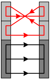
Figure B2: The color factor of this diagram is $3!\cdot 3$ since one has the valence circuit and an independent circuit.

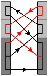
Figure B3: The color contractions in this diagram give a minus factor because of interchange of two valence quarks.

The second one has three crossings (they are degenerate in the drawing but it does not change anything considering one or three crossings since the important thing is that it is odd) and is thus negative. So is the third one with its unique crossing. The fourth diagram has four crossings and is thus positive. The last one has six crossings and is thus also positive.

Following rule 2 there must be $5!2!=240$ contractions. Indeed, there are 12 of the first and second types while there are 72 of the other ones. Thus we have $2\cdot 12+3\cdot 72=240$ contractions as expected.

The color factor of the first diagram is $3!\cdot 3\cdot 3=54$ since there are two independent circuits. The color factor of the second one is only $3!\cdot 3=18$ since there is only one independent circuit as one can see on Fig. B3. The third diagram has also a unique independent circuit and thus a color factor of $3!\cdot 3=18$. For the two last diagrams there are no more independent circuit and we have consequently a color factor of $3!=6$.

We close this appendix by considering the diagram in Fig. B3. Since two valence quarks are exchanged, it must belong to the fifth type of diagrams. There are seven crossings and thus a negative sign while the fifth type of diagrams is positive. In fact, for this particular diagram, the color contractions gives an additional minus sign since the third quark on the left is contracted with the second on the right $\epsilon^{\alpha_{1}\alpha_{2}\alpha_{3}}\epsilon_{\alpha_{1}\alpha_{3}\alpha_{2}}=-6$.

Bibliography

- [1] E. Fermi and C.N. Yang, Phys. Rev. 76 (1949) 1739.
- [2] S. Sakata, Prog. Theor. Phys. 16 (1956) 686.
-
[3]
E.D. Bloom et al., Phys. Rev. Lett. 23
(1969) 930;
M. Breidenbach et al., Phys. Rev. Lett. 23 (1969) 935. -
[4]
F.E. Close, An Introduction to Quarks and
Partons, Academic Press, London, 1979;
T. Muta, Foundations of Quantum Chromodynamics, World Scientific, Singapore, 1987;
R.G. Roberts, The Structure of the Proton, Cambridge University Press, Cambridge, 1990. - [5] J.D. Bjørken, Phys. Rev. 179 (1969) 1547.
-
[6]
R.P. Feynman, Phys. Rev. Lett. 23 (1969) 1415;
R.P. Feynman, Photon-Hadron Interactions, Benjamin, New York, 1972. - [7] M. Gell-Mann, Phys. Lett. 8 (1964) 214.
- [8] G. Zweig, CERN Reports, TH401 and TH412 (1964).
-
[9]
G. ’t Hooft, Proc. Colloquium on Renormalization of
Yang-Mills fields and Application to Particle Physics, ed. C.P.
Korthals-Altes, Marseilles, 1972;
D.J. Gross and F. Wilczek, Phys. Rev. Lett. 30 (1973) 1343;
H.D. Politzer, Phys. Rev. Lett. 30 (1973) 1346;
H. Fritzsch, M. Gell-Mann and H. Leutwyler, Phys. Lett. B46 (1973) 365. -
[10]
T.H.R. Skyrme, Proc. Roy. Soc. 260 (1961) 127;
T.H.R. Skyrme, Nucl. Phys. 31 (1962) 556;
A. Chodos, R.L. Jaffe, K. Johnson, C.B. Thorn and V.F. Weisskopf, Phys. Rev. D9 (1974) 3471;
A. Chodos, R.L. Jaffe, K. Johnson and C.B. Thorn, Phys. Rev. D10 (1974) 2599;
A. de Rujula, H. Georgi and S.L. Glashow, Phys. Rev. D12 (1975) 147;
T. DeGrand, R.L. Jaffe, K. Johnson and J. Kiskis, Phys. Rev. D12 (1975) 2060;
R. Friedberg and T.D. Lee, Phys. Rev. D16 (1977) 1096;
R. Friedberg and T.D. Lee, Phys. Rev. D18 (1978) 2623;
E. Witten, Nucl. Phys. B223 (1983) 422. - [11] E. Witten, Nucl. Phys. B223 (1983) 433.
-
[12]
N. Isgur and G. Karl, Phys. Rev. D18
(1978) 4187;
N. Isgur and G. Karl, Phys. Rev. D19 (1979) 2653;
N. Isgur and G. Karl, Phys. Rev. D20 (1979) 1191. -
[13]
M. Oka and K. Yakazaki, Phys. Lett. B90
(1980) 41;
M. Oka and K. Yakazaki, Prog. Theor. Phys. 66 (1981) 556;
M. Oka and K. Yakazaki, Prog. Theor. Phys. 66 (1981) 572;
A. Fäßler, F. Fernandez, G. Lübeck and K. Shimizu, Phys. Lett. B112 (1982) 201;
A. Fäßler, F. Fernandez, G. Lübeck and K. Shimizu, Nucl. Phys. A402 (1983) 555;
Y. Fujiwara and K.T. Hencht, Nucl. Phys. A444 (1985) 541;
S. Takeushi, K. Shimizu and K. Yazaki, Nucl. Phys. A504 (1989) 777;
F. Wang, G.H. Wu, L.J. Teng and T. Goldman, Phys. Rev. Lett. 69 (1992) 2901;
Z.Y. Zhang, A. Fäßler, U. Straub and L.Ya. Glozman, Nucl. Phys. A578 (1994) 573;
G.H. Wu, L.J. Teng, J.L. Ping, F. Wang and T. Goldman, Phys. Rev. C53 (1996) 1161;
Y. Fujiwara, C. Nakamoto and Y. Suzuki, Phys. Rev. Lett. 76 (1996) 2242. - [14] J.I. Friedman and H.W. Kendall, Annu. Rev. Nucl. Sci. B28 (1971) 240.
- [15] J.D. Bjørken and E.A. Paschos, Phys. Rev. 185 (1969) 1975.
- [16] J. Kuti and V.F. Weisskopf, Phys. Rev. D4 (1971) 3418.
-
[17]
E. Noether, Kgl. Ges. d. Wiss. Nachricten,
Math.-Phys. Klasse, Göttingen, 1918;
C. Itzykson and J.B. Zuber, Quantum Field Theory, McGraw-Hill, New York, 1985. - [18] J. Goldstone, Nuevo Cim. 19 (1961) 154.
- [19] D. Diakonov and V. Petrov, Nucl. Phys. B245 (1984) 259.
- [20] M.A. Schifman, A.I. Vainshyein and V.I. Zakharov, Nucl. Phys. B147 (1979) 385.
- [21] B.L. Ioffe, Nucl. Phys. B188 (1981) 317.
-
[22]
H. Yukawa, Proc. Phys. Math. Soc. Japan 17
(1935) 48;
J.L. Gammel and R.M. Thaler, Phys. Rev. 107 (1957) 291. -
[23]
F. Myhrer and J. Wroldsen, Rev. Mod. Phys. 60 (1988) 629;
L. Ya. Glozman, Nucl. Phys. A663/664 (2000) 103c. - [24] D. Bartz and Fl. Stancu, Phys. Rev. C63 (2001) 034001.
- [25] M.L. Goldberger and S.B. Treiman, Phys. Rev. 110 (1958) 1178.
- [26] V. Bernard, N. Kaiser and U.G. Meissner, Phys. Rev. D50 (1994) 6899.
- [27] A.M. Bernstein and C.N. Papanicolas, arXiv:0708.0008 [hep-ph].
- [28] R.L. Jaffe and X. Ji, Phys. Rev. Lett. 67 (1991) 552.
-
[29]
J.D. Bjørken, Phys. Rev. 148 (1966) 1467;
J.D. Bjørken, Phys. Rev. D1 (1966) 1376. -
[30]
M. Gourdin, Nucl. Phys. 38 (1972) 418;
J. Ellis and R.L. Jaffe, Phys. Rev. D9 (1974) 1444 [Erratum-ibid. D10 (1974) 1669]. -
[31]
R.L. Jaffe and A. Manohar, Nucl.
Phys. B337 (1990) 509;
X. Ji, Phys. Rev. Lett. 78 (1997) 610. -
[32]
S.J. Brodsky, J. Ellis and M. Karliner, Phys.
Lett. B206 (1988) 309;
J. Ellis and M. Karliner, Phys. Lett. B213 (1988) 73. -
[33]
J. Ashman et al. [EMC], Phys. Lett. B206
(1988) 364;
J. Ashman et al. [EMC], Nucl. Phys. 328 (1989) 1. - [34] G. Veneziano, Mod. Phys. Lett. A4 (1989) 1605.
-
[35]
S. Okubo, Phys. Lett. 5 (1963) 165;
J. Iizuka, Prog. Theor. Phys. Suppl. 37-38 (1966) 21;
J. Iizuka, K. Okada and O. Shito, Prog. Theor. Phys. 35 (1966) 1061. - [36] R.C. Hwa, Phys. Rev. D22 (1980) 759.
- [37] B.I. Abelev et al. [STAR Coll.], Phys. Rev. Lett. 97 (2006) 252001, hep-ex/0608030.
- [38] N. Bianchi, Talk givin at Pacific-SPIN07, July 30-August 2 2007, Vancouver BC, Canada, http://www.triumf.info/hosted/pacspin07/program.htm.
- [39] S. Forte and Y. Goto, hep-ph/0609127.
- [40] B. Lampe and E. Reya, Phys. Rept. 332 (2000) 1.
-
[41]
J. Gasser and H. Leutwyler, Ann. Phys. 136 (1981) 62;
J. Gasser and H. Leutwyler, Phys. Rept. 87 (1982) 77;
J. Gasser, H. Leutwyler and M.E. Sanio, Phys. Lett. B253 (1991) 252;
K. Abe et al., Phys. Lett. B405 (1997) 180;
G. Altarelli, Nucl. Phys. B496 (1997) 337;
T. Adams et al., hep-ex/9906038. -
[42]
B. Mueller et al. [SAMPLE Coll.], Phys.
Rev. Lett. 78 (1997) 3824;
R. Hasty et al. [SAMPLE Coll.], Science 290 (2000) 2117;
T.M. Ito et al. [SAMPLE Coll.], Phys. Rev. Lett. 92 (2004) 102003;
D.T. Spayde et al. [SAMPLE Coll.], Phys. Lett. B583 (2004) 79;
E.J. Beise, M.L. Pitt and D.T. Spayde, Prog. Part. Nucl. Phys. 54 (2005) 289. -
[43]
F.E. Maas et al. [A4 Coll.], Phys. Rev. Lett. 93
(2004) 022002;
F.E. Maas [A4 Coll.]et al., Phys. Rev. Lett. 94 (2005) 152001. -
[44]
K. Aniol et al. [HAPPEX Coll.], Phys. Rev. C69 (2004) 065501;
K. Aniol et al. [HAPPEX Coll.], Phys. Lett. B635 (2006) 275, nucl-ex/0506011;
K. Aniol et al. [HAPPEX Coll.], Phys. Rev. Lett. 96 (2006), 022003;
A. Acha. et al. [HAPPEX Coll.], Phys. Rev. Lett. 98 (2007) 032301, nucl-ex/0609002. - [45] D.S. Armstrong et al. [G0 Coll.], Phys. Rev. Lett. 95 (2005) 092001.
-
[46]
K.S. Kumar and P.A. Souder, Prog. Part. Nucl.
Phys. 45 (2000) S333;
D.H. Beck and B.R. Holstein, Int. J. Mod. Phys. E10 (2001) 1;
D.H. Beck and R.D. McKeown, Annu. Rev. Nucl. Part. Sci. 51 (2001) 189;
B.S. Zou and D.O. Riska, Phys. Rev. Lett. 95 (2005) 072001;
C.S. An, B.S. Zou and D.O. Riska, Phys. Rev. C73 (2006) 035207;
D.O. Riska and B.S. Zou, Phys. Lett. B36 (2006) 265;
R. Bijker, J. Phys. G32 (2006) L49. -
[47]
B. Adeva et al. [SMC], Phys. Lett. B369 (1996)
93;
B. Adeva et al. [SMC], Phys. Lett. B420 (1998) 180. -
[48]
A. Airapetian et al. [HERMES Coll.],
Phys. Rev. Lett. 92 (2004) 012005;
A. Airapetian et al. [HERMES Coll.], Phys. Rev. D71 (2005) 012003;
H.E. Jackson, hep-ex/0601006. -
[49]
V.Yu. Alexakhin et al., Phys. Lett. B647 (2007) 8;
A. Korzenev [COMPASS Coll.], arXiv:0704.3600 [hep-ex]. -
[50]
S. Kumano, Phys. Rept. 303 (1998) 183;
G.T. Garvey and J.C. Peng, Prog. Part. Nucl. Phys. 47 (2001) 203;
A.L. Kataev, Talk given at the 11th Lomonosov COnference on Elementary Particle physics, August 21-27 2003, Moscow, Russia, hep-ph/0311091. - [51] M. Arneodo et al. [NMC], Phys. Rev. D50 (1994) 1.
- [52] K. Gottfried, Phys. Rev. Lett. 18 (1967) 1174.
-
[53]
E. Reya, Rev. Mod. Phys. 46 (1974) 545;
R. Koch, Z. Phys. C15 (1982) 161. -
[54]
M.G. Olsson, W.B. Kafmann, N Newslett. 16 (2002) 382;
P. Schweitzer, Eur. Phys. J. A22 (2004) 89. - [55] F. Olness et al., Eur. Phys. J. C40 (2005) 145.
- [56] J. Ellis and M. Karliner, hep-ph/9601280.
-
[57]
R. Beck et al., Phys. Rev. C61 (2000)
035204, nucl-ex/9908017;
G. Blanpied et al., Phys. Rev. C64 (2001) 025203;
G.A. Warren et al., Phys. Rev. C58 (1998) 3722;
C. Mertz et al., Phys. Rev. Lett. 86 (2001) 2963;
C. Kunz et al., Phys. Lett. B564 (2003) 21, nucl-ex/0302018;
N.F. Sparveris et al., Phys. Rev. Lett. 94 (2005) 022003;
K. Joo et al., Phys. Rev. Lett. 88 (2002) 122001, hep-ex/0110007;
V.V. Frolov et al., Phys. Rev. Lett. 82 (1999) 45, hep-ex/9808024;
T. Pospischil et al., Phys. Rev. Lett. 86 (2001) 2959;
P. Bartsch et al., Phys. Rev. Lett. 88 (2002) 142001;
M. Ungaro et al., Phys. Rev. Lett. 97 (2006) 112003, hep-ex/0606042;
D. Elsner et al., Eur. Phys. J. A27 (2006) 91;
A.M. Sandorfi et al., Nucl. Phys. A629 (1998) 171C, hep-ex/0606042;
S. Stave et al., nucl-ex/0604013. - [58] D. Drechsel and L. Tiator, editors, Proceedings of the Workshop on the Physics of Excited Nucleons, World Scientific, 2001.
- [59] C. Becchi and G. Morpugo, Phys. Lett. 16 (1965) 16.
- [60] C.N. Papanicolas, Eur. Phys. J. A18 (2003) 141.
- [61] S. Capstick and G. Karl, Phys. Rev. D41 (1990) 2767.
- [62] S.L. Glashow, Physica A96 (1979) 27.
-
[63]
R. Koniuk and N. Isgur, Phys. Rev. D21
(1980) 1868;
D. Drechsel and M.M. Giannini, Phys. Lett. 143B (1984) 329. - [64] A.M. Bernstein, Eur. Phys. J. A17 (2003) 349.
-
[65]
N. Isgur, G. Karl and R. Koniuk, Phys. Rev. D25 (1982) 2394;
S.S. Gershtein and G.V. Jikia, Sov. J. Nucl. Phys. 34 (1981) 870 [Yad. Fiz. 34 (1981) 1566];
S.A. Gogilidze, Yu.S. Surovtsev and F.G. Tkebuchava, Yad. Fiz. 45 (1987) 1085. -
[66]
A. Wirzba and W. Weise, Phys. Lett. B188
(1987) 6;
E. Jenkins, X.D. Ji and A.V. Manohar, Phys. Rev. Lett. 89 (2002) 242001, hep-ph/0207092. - [67] K. Bermuth, D. Drechsel, L. Tiator and J.B. Seaborn, Phys. Rev. D37 (1988) 89.
-
[68]
T.A. Gail and T.R. Hemmert, Eur. Phys. J. A28
(2006) 91, nucl-th/0512082;
V. Pascalutsa and M. Vanderhaeghen, Phys. Rev. D73 (2006) 034003, hep-ph/0512244. - [69] C. Alexandrou, Ph. de Forcrand, H. Neff, J.W. Negele, W. Schroers and A. Tsapalis, Phys. Rev. Lett. 94 (2005) 021601, hep-lat/0409122.
- [70] V. Pascalutsa, M. Vanderhaeghen and S.N. Yang, Phys. Rept. 437 (2007) 125, hep-ph/0609004.
-
[71]
R.L. Jaffe, Phys. Rev. D15 (1977) 267;
preprint SLAC-PUB-1774;
D. Strottman, Phys. Rev. D20 (1979) 748. - [72] H.J. Lipkin, Nucl. Phys. A625 (1997) 207.
- [73] Ya. Azimov, K. Goeke and I. Strakovsky, arXiv:0704.3045 [hep-ph].
-
[74]
K.H. Hicks, Prog. Part. Nucl. Phys. 55 (2005) 647,
hep-ex/0504027;
M. Danilov, Talk given at Les Rencontres de Physique de la Vallée d’Aoste, hep-ex/0509012;
V.D. Burkert, Int. J. Mod. Phys. A21 (2006) 1764, hep-ph/0510309;
D. Diakonov, Talks given at Quarks 2006, May 19-26 2006, St Petersburg, Russia and at Quark Confinement and Hadron Spectrum VII, September 2-7 2006, Ponta Delgada, Portugal, hep-ph/0610166;
K. Hicks, hep-ph/0703004;
M. Danilov and R. Mizuk, arXiv:0704.3531 [hep-ex]. - [75] D. Diakonov, V. Petrov and M.V. Polyakov, Z. Phys. A359 (1997) 305, hep-ph/9703373.
- [76] D. Diakonov and V. Petrov, Phys. Rev. D72 (2005) 074009, hep-ph/0505201.
- [77] M.V. Polyakov and A. Rathke, Eur. phys. J. A18 (2003) 691, hep-ph/0303138.
- [78] R.A. Arndt, Y.I. Azimov, M.V. Polyakov, I.I. Strakovsky and R.L. Workman, Phys. Rev. C69 (2004) 035208, nucl-th/0312126.
-
[79]
V. Kuznetsov [GRAAL Coll.],
hep-ex/0409032;
V. Kuznetsov [GRAAL Coll.], hep-ex/0606065;
V. Kuznetsov et al., Phys. Lett. B647 (2007) 23. - [80] A. Fix, L. Tiator and M.V. Polyakov, Eur. Phys. J. A32 (2007) 311.
- [81] J. Kasagi, Talk given at Yukawa International Smeinar YKIS2006, November 20- December 8 2006, Kyoto, Japan, http://www2.yukawa.kyoto-u.ac.jp ykis06/.
-
[82]
J. Jaegle, Talk given at Workshop on the Physics of
Excited Nucleons NSTAR2005, October 12-15 2005, Tallahassee, FL,
USA, World Scientific 2006, p. 340;
B. Krusche et al., Talk given at International Workshop on Eta physics, May 8-12 2006, Jülich, Germany, nucl-th/0610011. - [83] V. Petrov and M. Polyakov, hep-ph/0307077.
- [84] C. Lorcé, Phys. Rev. D74 (2006) 054019, hep-ph/0603231.
- [85] C. Lorcé, arXiv:0708.3139 [hep-ph].
- [86] C. Lorcé, arXiv:0708.4168 [hep-ph].
- [87] C. Lorcé and M.V. Polyakov, two papers in preparation.
- [88] P.A.M. Dirac, The Principles of Quantum Mechanics, 4th ed., Oxford Univ. Press, Oxford, 1958.
- [89] P.A.M. Dirac, Rev. Mod. Phys. 21 (1949) 392.
-
[90]
J.K. Lubanski, Physica IX (1942) 310;
V. Bargmann and E.P. Wigner, Proc. Nat. Acad. Sci. (USA) 34 (1948) 211. - [91] J.B. Kogut and D.E. Soper, Phys. Rev. D1 (1970) 2901.
- [92] F. Coester, Prog. Part. Nucl. Phys. 29 (1992) 1.
- [93] M. Fuda, Ann. Phys. (N.Y.) 197 (1990) 265.
-
[94]
X.D. Ji, J. Phys. G24 (1998) 1181;
A.V. Radyushkin, hep-ph/0101225;
K. Goeke, M.V. Polyakov and M. Vanderhaeghen, Prog. Part. Nucl. Phys. 47 (2001), hep-ph/0106012;
A.V. Belitsky, D. Muller and A. Kirchner, Nucl. Phys. B629 (2002) 323, hep-ph/0112108;
M. Diehl, Phys. Rept. 388 (2003) 41;
B.C. Tiburzi, nucl-th/0407005. -
[95]
S.J. Brodsky, M. Diehl and D.S. Hwang, Nucl. Phys. B569 (2001) 99;
M. Diehl, T. Feldmann, R. Jakob and P. Kroll, Nucl. Phys. B596 (2001) 33 [Erratum-ibid. B605 (2001) 647]. -
[96]
B.V. Berestetsky and M.V. Terentev, Sov. J.
Nucl. Phys. 24 (1976) 547 [Yad. Fiz. 24 (1976) 1044];
B.V. Berestetsky and M.V. Terentev, Sov. J. Nucl. Phys. 25 (1977) 347 [Yad. Fiz. 25 (1977) 653]. - [97] P.L. Chung and F. Coester, Phys. Rev. D44 (1991) 229.
-
[98]
S.D. Drell and T.M. Yan, Phys. Rev. Lett. 24
(1970) 181;
G. West, Phys. Rev. Lett. 24 (1970) 1206. - [99] S. Fubini and G. Furlan, Physics 1 (1965) 229.
- [100] S. Weinberg, Phys. Rev. 150 (1966) 1313.
- [101] L. Susskind and G. Frye, Phys. Rev. 164 (1967) 1535.
- [102] K. Bardakci and M.B. Halpern, Phys. Rev. 176 (1968) 1786.
-
[103]
S.D. Drell, D. Levy and T.M. Yan, Phys. Rev. 187 (1969) 2159;
S.D. Drell, D. Levy and T.M. Yan, Phys. Rev. D1 (1970) 1035;
S.D. Drell, D. Levy and T.M. Yan, Phys. Rev. D1 (1970) 1617. - [104] V. De Alfaro, S. Fubini, G. Furlan and C. Rosetti, Currents in Hadron Physics, Amsterdam, North Holland, 1973.
-
[105]
G.P. Lepage and S.J. Brodsky, Phys. Rev. Lett. 43 (1979) 545;
G. Lepage and S. Brodsky, Phys. Rev. D22 (1980) 2157;
V.A. Karmanov, Nucl. Phys. B166 (1980) 378;
B.C. Tiburzi, nucl-th/0407005. -
[106]
F. Coester and W.N Polyzou, Phys. Rev. D26
(1982) 1348;
P.L. Chung, F. Coester, B.D. Keister and W.N. Polyzou, Phys. Rev. C37 (1988) 2000;
S.J. Brodsky, G. McCartor, H.C. Pauli and S.S. Pinsky, in Particle World 3 (1993) 203. - [107] H.J. Melosh, Phys. Rev. D9 (1974) 1095.
- [108] S.J. Brodksy and J.R. Primack, Annals Phys. 52 (1960) 315.
- [109] S.J. Brodsky, J.R. Hiller, D.S. Hwang and V.A. Karmanov, Phys. Rev. D69 (2004) 076001, hep-ph/0311218.
- [110] S.J. Brodsky, H.C. Pauli and S.S. Pinsky, Phys. Rept. 301 (1998) 299.
- [111] G. Adkins, C. Nappi and E. Witten, Nucl. Phys. B228 (1983) 552.
-
[112]
D. Diakonov and V. Petrov, Phys. Lett. B147
(1984) 351;
D. Diakonov and V. Petrov, Nucl. Phys. B272 (1986) 457. -
[113]
D. Diakonov and V. Petrov, JETP Lett. 43 (1986) 57 [Pisma Zh. Eksp. Teor. Fiz. 43 (1986) 57];
D. Diakonov, V. Petrov and P. Pobylitsa, Nucl. Phys. B306 (1988) 809;
D. Diakonov and V. Petrov, in Handbook of QCD, ed. M. Shifman, World Scientific, Singapore (2001), vol. 1, p. 359, hep-ph/0009006. - [114] D. Diakonov, V. Petrov and M. Praszalowicz, Nucl. Phys. B323 (1989) 53.
- [115] C. Christov, A. Blotz, H.-C. Kim, P. Pobylitsa, T. Watabe, Th. Meissner, E. Ruiz Arriola and K. Goeke, Prog. Part. Nucl. Phys. 37 (1996) 91, hep-ph/9604441.
-
[116]
R. Alkofer, H. Reinhardt and H. Weigel, Phys. Rept. 265 (1996)
139;
D. Diakonov and V. Petrov, nucl-th/0009006, Contribution to the Festschrift in honor of B.L. Ioffe;
M. Praszalowicz and K. Goeke, Acta Phys. Pol. B36 (2005) 2255. -
[117]
V.Yu. Petrov, P.V. Pobylitsa, M.V. Polyakov, I.
Borning, K. Goeke and C. Weiss, Phys. Rev. D57 (1998) 4325;
M. Penttinen, M.V. Polyakov and K. Goeke, Phys. Rev. D62 (2000) 014024. -
[118]
D. Diakonov, V. Petrov, P. Pobylitsa, M. Polyakov
and C. Weiss, Nucl. Phys. B480 (1996) 341,
hep-ph/9606314;
D. Diakonov, V. Petrov, P. Pobylitsa, M. Polyakov and C. Weiss, Phys. Rev. D56 (1997) 4069, hep-ph/9703420. -
[119]
H. Weigel, L. Gamberg and H. Reinhardt, Mod. Phys. Lett. A11 (1996) 3021;
H. Weigel, L. Gamberg and H. Reinhardt, Phys. Lett. B399 (1997) 287;
H. Weigel, L. Gamberg and H. Reinhardt, Phys. Rev. D55 (1997) 6910;
M. Wakamatsu and T. Kubota, Phys. Rev. D57 (1998) 5755;
P.V. Pobylitsa, M.V. Polyakov, K. Goeke, T. Watabe and C. Weiss, Phys. Rev. D59 (1999) 034024;
M. Wakamatsu and T. Kubota, Phys. Rev. D60 (1999) 034020. -
[120]
S. Kahana, G. Ripka and V. Soni, Nucl. Phys.
A415 (1984) 351;
S. Kahana and G. Ripka, Nucl. Phys. A429 (1984) 462. - [121] D. Diakonov and V. Petrov, Annalen des Phys. 13 (2004) 637, hep-ph/0409362.
- [122] E.H. Lieb, Rev. Mod. Phys. 53 (1981) 603.
- [123] M.S. Birse and M.K. Banerjee, Phys. Lett. B136 (1984) 284.
-
[124]
E. Guadagnini, Nucl. Phys. B236 (1984)
35;
L.C. Biedenharn, Y. Dothan and A. Stern, Phys. Lett. B146 (1984) 289;
P.O. Mazur, M.A. Nowak and M. Praszalowicz, Phys. Lett. B147 (1984) 137;
A.V. Manohar, Nucl. Phys. B248 (1984) 19;
M. Chemtob, Nucl. Phys. B256 (1985) 600;
S. Jain and S.R. Wadia, Nucl. Phys. B258 (1985) 713;
D. Diakonov and V. Petrov, Baryons as solitons, preprint LNPI-967 (1984), published in Elementary Particles, Proc. 12th ITEP Winter School, Energoatomizdat, Moscow, Russia (1985) pp. 50-93. - [125] A. Blotz, D. Diakonov, K. Goeke, N.W. Park, V. Petrov and P. Pobylitsa, Nucl. Phys. A555 (1993) 765, Appendix A.
- [126] Y. Oh and H. Kim, Phys. Rev. D70 (2004) 094022, hep-ph/0405010.
- [127] J.R. Ralston and D.E. Soper, Nucl. Phys. B152 (1979) 109.
- [128] R.L. Jaffe and X. Ji, Nucl. phys. B375 (1992) 527.
-
[129]
J.C. Collins, Nucl. Phys. B394 (1993) 169;
J.C. Collins, Nucl. phys. B396 (1993) 161, hep-ph/9208213. - [130] V. Barone, A. Drago and P.G. Ratcliffe, Phys. Rept. 359 (2002) 1, hep-ph/0104283.
- [131] N. Cabibbo, Phys. Rev. Lett. 10 (1963) 531.
-
[132]
D.B. Lichtenber, Unitary symmetry and elementary
particles, Academic Press, New York and London, 1970;
Yu. V. Novozhilov, Introduction to elementary particle physics, Pergamon Press, 1975;
V. Guzey and M. Polyakov, hep-ph/0512355. - [133] S. Coleman and S.L. Glashow, Phys. Rev. Lett. 6 (1961) 423.
- [134] V. Guzey and M. Polyakov, hep-ph/0512355.
-
[135]
D. Jido and W. Weise, Phys. Rev. C72 (2005) 045203;
P. Wang, D.B. Leinweber, A.W. Thomas and R.D. Young, hep-ph/0701082. - [136] R. Flores-Mendieta, E. Jenkins and A.V. Manohar, Phys. Rev. D58 (1998) 094028.
- [137] D.B. Kaplan and A. Manohar, Nucl. Phys. B310 (1988) 527.
- [138] V. Dmitrašinović, Phys. Rev. D71 (2005) 094003.
- [139] M.A.B. Bég, B.W. Lee and A. Pais, Phys. Rev. Lett. 13 (1964) 514.
-
[140]
D.A. Ross and C.T. Sachrajda, Nucl. Phys. B149 (1979) 497;
A.L. Kataev, A.V. Kotikov, G. Parente and A.V. Sidirov, Phys. Lett. B388 (1996) 179. - [141] R.S. Towell et al. [FNAL E866/NuSea Coll.], Phys. Rev. D64 (2001) 052002, hep-ex/0103030.
- [142] K. Ackerstaff et al. [HERMES Coll.], Phys. Rev. Lett. 81 (1998) 5519.
-
[143]
H. Abramowicz et al. [CDHS Coll.], Z. Phys. C15 (1982) 19;
H. Abramowicz et al. [CDHS Coll.], Z. Phys. C17 (1983) 283;
C. Foudas et al. [CCFR Coll.], Phys. Rev. Lett. 64 (1990) 1207;
S.A. Rabinowitz et al., Phys. Rev. Lett. 70 (1993) 134;
W.C. Leung et al., Phys. Lett. B317 (1993) 655;
A.O. Bazarko et al., Z. Phys. C65 (1995) 189. - [144] A.I. Signal and A.W. Thomas, Phys. Lett. B191 (1987) 205.
-
[145]
S.J. Brodsky and B.Q. Ma, Phys. Lett. B381
(1996) 317;
H.R. Christiansen and J. Magnin, Phys. Lett. B445 (1998) 8;
F.G. Cao and A.I. Signal, Phys. Rev. D60 (1999) 074021. -
[146]
A.O. Bazarko et al., Z. Phys. C65
(1995) 189;
F. Olness et al., Eur. Phys. J. C40 (2005) 145. -
[147]
S. Davidson, S. Forte, P. Gambino, N. Rius ans
A. Strumia, JHEP 0202 (2002) 037;
S. Kretzer, F. Olness, J. Pumplin, D. Stump, W.K. Tung and M.H. Reno, Phys. Rev. Lett. 93 (2004) 041802. - [148] G.P. Zeller et al. [NuTeV Coll.], Phys. Rev. D65 (2002) 111103(R).
- [149] Y.A. Siminov and M.A. Trusov, hep-ph/0506058.
- [150] B.W. Filippone and X.D. Ji, Adv. Nucl. Phys. 26 (2001) 1.
-
[151]
J. Ellis, R.A. Flores and S. Ritz, Phys. Lett. B198
(1987) 393;
K. Griest, Phys. Rev. D38 (1988) 2357;
J. Ellis and R.A. Flores, Nucl. Phys. B307 (1988) 883;
J. Ellis and R.A. Flores, Phys. Lett. B263 (1991) 259;
J. Ellis and R.A. Flores, Nucl. Phys. B400 (1993) 25. - [152] M. Ademollo and R. Gatto, Phys. Rev. Lett. 13 (1964) 264.
- [153] J.C. Peng, Eur. phys. J. A18 (2003) 395.
-
[154]
B.Q. Ma, J. Phys. G17 (1991) L53;
B.Q. Ma and Q.R. Zhang, Z. Phys. C58 (1993) 479. - [155] S.J. Brodsky and F. Schlumpf, Phys. Lett. B329 (1994) 111.
- [156] C. Bourrely, F. Buccella, J. Soffer, Eur. Phys. J. C41 (2005) 327.
- [157] D. de Florian, G.A. Navarro and R. Sassot, Phys. Rev. D71 (2005) 094018.
- [158] H.C. Kim, M. Praszalowicz and K. Goeke, Acta Phys. Polon. B32 (2001) 1343, hep-ph/0007022.
- [159] S.D. Bass, Rev. Mod. Phys. 77 (2005) 1257.
- [160] W.M. Yao et al., J. Phys. G33 (2006), 1.
- [161] T. Yamanishi, arXiv:0705.4340 [hep-ph].
- [162] P.G. Ratcliffe, Czech. J. Phys. 54 (2004) B11.
- [163] L.B. Okun, Leptons and Quarks, Nauka, Moscow (1981), ch. 8.
-
[164]
G.R. Goldstein and M.J. Moravcsik, Ann.
Phys. (N.Y.) 98 (1976) 128;
G.R. Goldstein and M.J. Moravcsik, Ann. Phys. (N.Y.) 142 (1982) 219;
G.R. Goldstein and M.J. Moravcsik, Ann. Phys. (N.Y.) 195 (1989) 213. - [165] X. Artru and M. Mekhfi, Z. Phys. C45 (1990) 669.
-
[166]
A. Hayashigaki, Y. Kanazawa and Y. Koike, Phys.
Rev. D56 (1997) 7350, hep-ph/9707208;
W. Vogelsang, Phys. Rev. D57 (1998) 1886, hep-ph/9706511. - [167] I.C. Cloët, W. Bentz and A.W. Thomas, arXiv:0708.3246 [hep-ph].
- [168] J. Soffer, Phys. Rev. Lett. 74 (1995) 1292.
- [169] J. Soffer, R.L. Jaffe and X. Ji, Phys. Rev. D52 (1995) 5006.
- [170] I. Schmidt and J. Soffer, Phys. Lett. B407 (1997) 331.
- [171] M. Anselmino, M. Boglione, U. D’Alesio, A. Kotzinian, F. Murgia, A. Prokudin and C. Turk, Phys. Rev. D75 (2007) 054032, hep-ph/0701006.
-
[172]
H.Y. Gao, Int. J. Mod. Phys. E12 (2003) 1 [Erratum-ibid. E12 (2003) 567],
nucl-ex/0301002;
C.E. Hyde-Wright and K. de Jager, Ann. Rev. Nucl. Part. Sci. 54 (2004) 217, nucl-ex/0507001;
J. Arrington, C.D. Roberts and J.M. Zanotti, nucl-th/0611050;
C.F. Perdrisat, V. Punjabi and M. Vanderhaeghen, Prog. Part. Nucl. Phys. 59 (2007) 694, hep-ph/0612014. - [173] F.J. Ernst, R.G. Sachs and K.C. Wali, Phys. Rev. 119 (1960) 1105.
- [174] R.G. Sachs, Phys. Rev. 126 (1962) 2256.
- [175] S.J. Brodsky and S.D. Drell, Phys. Rev. D22 (1980) 2236.
- [176] W. Rarita and J. Schwinger, Phys. Rev. 60 (1941) 61.
- [177] F. Schlumpf, Phys. Rev. D48 (1993) 4478, hep-ph/9305293.
- [178] H.F. Jones and M.D. Scadron, Annals Phys. 81 (1973) 1.
- [179] F. Cardarelli, E. Pace, G. Salmè and S. Simula, Nucl. Phys. A623 (1997) 361.
- [180] A. Silva, H.C. Kim and K. Goeke, Phys. Rev. D65 (2001) 014016.
- [181] B.D. Keister, Phys. Rev. D49 (1994) 1500.
- [182] V.A. Karmanov and J.F. Mathiot, Nucl. Phys. A602 (1996) 388.
-
[183]
M. Malheiro and W. Melnitchouk, Phys. Rev. C56 (1997) R2373, hep-ph/9709307;
W. Melnitchouk and M. Malheiro, Phys. Lett. B451 (1999) 224, hep-ph/9901321. - [184] D.B. Leinweber, T. Draper and R.M. Woloshyn, Phys. Rev. D46 (1992) 3067.
-
[185]
F. Schlumpf, Phys. Rev. D48 (1993) 4478;
J. Linde and H. Snellman, Phys. Rev. D53 (1996) 2337. - [186] S.T. Hong and G.E. Brown, Nucl. Phys. A580 (1994) 3459.
- [187] M.N. Butler, M.J. Savage and R.P. Springer, Phys. Rev. D49 (1994) 408.
-
[188]
F.X. Lee, Phys. Lett. B419 (1998) 14;
F.X. Lee, Phys. Rev. D57 (1998) 1801;
S.T. Hong, hep-ph/0702162. - [189] J. Linde, T. Ohlsson and H. Snellman, Phys. Rev. D57 (1998) 5916.
-
[190]
G.S. Yang, H.C. Kim, M. Praszalowicz and K. Goeke,
Phys. Rev. D70 (2004) 114002;
K. Goeke, H.C. Kim, M. Praszalowicz and G.S. Yang, Prog. Part. Nucl. Phys. 55 (2005) 350, hep-ph/0411195;
Z.G. Wang, W.M. Wang and S.L. Wan, J. Phys. G31 (2005) 703;
Z.G. Wang and R.C. Hu, hep-ph/0504273. - [191] A. Bohr and B. Mottelson, Nuclear structure II, Benjamin, Reading, MA, 1975.
-
[192]
C. Alexandrou, P. de Forcrand and A. Tsapalis,
Phys. Rev. D66 (2002) 094503, hep-lat/0206026;
C. Alexandrou, Nucl. Phys. Proc. Suppl. 128 (2004) 1, hep-lat/0311007. - [193] C. Alexandrou, G. Koutsou, H. Neff, J.W. Negele, W. Schroers and A. Tsapalis, arXiv:0710.4621 [hep-lat].
- [194] V. Pascalutsa and M. Vanderhaeghen, Phys. Rev. Lett. 95 (2005) 232001, hep-ph/0508060.
-
[195]
L. Tiator, D. Drechsel, O. Hanstein, S.S. Kamalov and S.N.
Yang, Nucl. Phys. A689 (2001) 205, nucl-th/0012046;
T. Sato and T.-S. H. Lee, Phys. Rev. C63 (2001) 055201;
L. Tiator, D. Drechsel, S.S. Kamalov and S.N. Yang, Eur. Phys. J A17 (2003) 357. - [196] S. Nam, K.-S. Choi, A. Hosaka and H.-C. Kim, arXiv:0704.3101 [hep-ph].
-
[197]
H.C. Kim, M. Polyakov, M. Praszalowicz, G.S. Yang and
K. Goeke, Phys. Rev. D71 (2005) 094023,
hep-ph/0506236;
H.C. Kim, G.S. Yang and K. Goeke, arXiv:0704.1777 [hep-ph]. - [198] Y. Azimov, V. Kuznetsov, M. Polyakov and I. Strakovsky, Eur. Phys. J. A25 (2005) 325, hep-ph/0506236.