Genuine Tripartite Entanglement in a Spin-Star Network at Thermal Equilibrium

Abstract

In a recent paper [M. Huber et al, Phys. Rev. Lett. 104, 210501 (2010)] new criteria to find out the presence of multipartite entanglement have been given. We exploit these tools in order to study thermal entanglement in a spin-star network made of three peripheral spins interacting with a central one. Genuine tripartite entanglement is found in a wide range of the relevant parameters. A comparison between predictions based on the new criteria and on the tripartite negativity is also given.

I Introduction

Entanglement has been widely studied for decades: criteria to find out the presence of bipartite entanglement in a quantum state are well known ref:Revealing_Bipartite , and, for systems with few degrees of freedom, it can be quantified ref:Wootters , whether the relevant state is pure or mixed. The analysis of multipartite entanglement is a more complicated task. For example, there have been many proposals of tripartite entanglement quantifiers ref:TripQuantify-1 ; ref:TripQuantify-2 ; ref:TripQuantify-3 ; ref:TripQuantify-4 and witnesses ref:TripWitnesses-1 ; ref:TripWitnesses-2 ; ref:TripWitnesses-3 , but none of such contributions have given a definitive solution to the problem of singling out and quantifying this type of correlations ref:Fazio2008 . The three-tangle has been considered a good tool able to quantify tripartite entanglement in pure states ref:TripQuantify-1 , but recently it has been criticized ref:DoesThreeTangle . Difficulties grow up when the system is described by a mixed state. Indeed, many of the proposals previously mentioned are valid only for pure states. An interesting tool for detecting tripartite correlations in mixed states has been presented by Sabin and Garcia-Alcaine ref:Sabin2008 , but the tripartite negativity they introduced (i.e., the geometric mean of the three negativities associated to the three possible bipartitions of a tripartite system) is not able to tell a genuine tripartite entangled state from a state which is biseparable in a generalized sense. Very recently, Huber et al ref:Huber2010 have given a set of relations that provide sufficient conditions to assert the presence of multipartite entanglement in an indisputable way, whether the state under scrutiny is pure or mixed. The basic idea of such criteria is to exclude the presence of any form of biseparability, in connection with all the possible bipartitions.

Over the last decade, the concept of thermal entanglement has emerged by investigating the presence of quantum correlations in quantum systems at thermal equilibrium ref:Arnesen2001 . In this context, the existence of quantum correlations have been put in connection with phase transitions ref:Osterloh2002 ; ref:Osborne2002 . Thermal entanglement has been studied in spin chains described by Heisenberg models ref:Gong2009 , in atom-cavity systems ref:Wang2009 , in simple molecular models ref:Pal2010 , and has been proposed as a resource in quantum teleportation protocols ref:Zhou2009 . Nonclassical and nonlocal correlations in thermalized quantum systems have been investigated ref:Werlang2010 ; ref:Souza2009 .

Thermal entanglement has been studied in spin-star networks. For instance, Hutton and Bose ref:Hutton2004 have analyzed the zero-temperature properties of such quantum systems, bringing to light interesting properties related to the parity of the number of outer (peripheral) spins. Recently, Wan-Li et al have studied the thermal entanglement in a spin-star network with three peripheral spins ref:Wan-Li2009 , evaluating pairwise entanglement between all possible couples of spins. More recently, Anzà et al ref:Anza2010 have analyzed tripartite correlations in a similar system, exploiting the tripartite negativity. Nevertheless, as already pointed out, such a tool cannot distinguish between tripartite entanglement and generalized biseparability.

In this paper, we investigate tripartite entanglement in the same system analyzed by Anzà et al, but exploiting the new criteria introduced by Huber et al. To this end, in the next section we summarize the results of ref ref:Huber2010 and specialize them to the three-spin case. In the third section we apply these tools to a thermalized spin-star network made of three peripheral spins interacting with a central one, bringing to light the presence of genuine tripartite thermal entanglement. Finally, in the last section, we discuss our results and give some conclusive remarks.

II Detection of Tripartite Entanglement

In a recent paper by Huber et al ref:Huber2010 , it has been shown that given a biseparable density operator $\rho$ acting on the Hilbert space $\cal H$, whether corresponding to pure or mixed state, for any completely separable state $\left|\Psi\right\rangle$ of the duplicated Hilbert space ${\cal H}\otimes{\cal H}$, it turns out that

$${\cal Q}(\rho,\Psi)=\sqrt{\left\langle\Psi\right|\,\rho^{\otimes 2}\,\Pi\,\left|\Psi\right\rangle}$$

$$\,\,-\sum_{i}\sqrt{\left\langle\Psi\right|\,(\Pi_{A_{i}}\otimes\mathbf{1}_{B_{i}})^{\dagger}\,\rho^{\otimes 2}\,(\Pi_{A_{i}}\otimes\mathbf{1}_{B_{i}})\,\left|\Psi\right\rangle}\leq 0\,,$$

(1)

where $i$ runs over all possible bipartitions of the system. The operator $\Pi$ performs swapping between the two parts of the duplicated Hilbert space, in the following way:

$$\left|\psi_{1}\right\rangle\otimes\left|\psi_{2}\right\rangle\,\epsilon\,{\cal H}\otimes{\cal H}\Rightarrow\Pi\left|\psi_{1}\right\rangle\otimes\left|\psi_{2}\right\rangle=\left|\psi_{2}\right\rangle\otimes\left|\psi_{1}\right\rangle\,.$$ (2)

Moreover, for a bipartition of the system $(A_{i},B_{i})$ and any separable state $\left|\Psi\right\rangle=\left|\psi_{A_{i}}\right\rangle\otimes\left|\psi_{B_{i}}\right\rangle\otimes\left|\chi_{A_{i}}\right\rangle\otimes\left|\chi_{B_{i}}\right\rangle\,\epsilon\,$ ${\cal H}\otimes{\cal H}$, one has:

$$(\Pi_{A_{i}}\otimes\mathbf{1}_{B_{i}})\left|\Psi\right\rangle=\left|\chi_{A_{i}}\right\rangle\otimes\left|\psi_{B_{i}}\right\rangle\otimes\left|\psi_{A_{i}}\right\rangle\otimes\left|\chi_{B_{i}}\right\rangle\,.$$ (3)

On the basis of (1), the occurrence of the condition ${\cal Q}>0$ for some trial state $\left|\Psi\right\rangle$ guarantees that state $\rho$ possesses genuine multipartite entanglement, in the sense that it is neither simply biseparable nor biseparable in a generalized sense (i.e., a state of the form $\rho=\sum_{i}\,p_{i}\,\rho_{A_{i}}\otimes\rho_{B_{i}}$). Therefore, after introducing the positive part of ${\cal Q}$,

$${\cal C}(\rho,\Psi)=\max[0,{\cal Q}(\rho,\Psi)]\,,$$ (4)

for a finite-dimensional Hilbert space, we can use the following condition,

$${\cal I}(\rho)=\int d\Psi\,{\cal C}(\rho,\Psi)>0\,,$$ (5)

as a sufficient condition to assert that $\rho$ is a multipartite ${\it entangled}$ state. In (5) the integration is meant over all possible completely separable states of the ${\cal H}\otimes{\cal H}$ Hilbert space. This means that, if the state $\left|\Psi\right\rangle$ depends on $P$ parameters, $q_{1}$, … $q_{P}$, one has $d\Psi=\prod_{k=1}^{P}\mathrm{d}q_{k}$.

Let us specialize this analysis to a three-spin system. In order to afford numerical calculation, we prevent integration over all possible trial states, and we consider only the special case

$$\left|\Psi(\theta,\phi,\eta,\xi)\right\rangle = \left|\theta,\phi\right\rangle\otimes\left|\theta,\phi\right\rangle\otimes\left|\theta,\phi\right\rangle$$ (6)

$$\otimes \left|\eta,\xi\right\rangle\otimes\left|\eta,\xi\right\rangle\otimes\left|\eta,\xi\right\rangle\,,$$

where

$$\left|\alpha,\beta\right\rangle=\cos\alpha\left|0\right\rangle+e^{-i\beta}\sin\alpha\left|1\right\rangle\,.$$ (7)

This choice gives rise to the following expression for the quantity ${\cal Q}$:

$${\cal Q}(\rho,\theta,\phi,\eta,\xi) = |\left\langle\theta,\phi\right|\left\langle\theta,\phi\right|\left\langle\theta,\phi\right|{\rho}\left|\eta,\xi\right\rangle\left|\eta,\xi\right\rangle\left|\eta,\xi\right\rangle|$$ (8)

$$- \sqrt{\left\langle\eta,\xi\right|\left\langle\eta,\xi\right|\left\langle\theta,\phi\right|{\rho}\left|\theta,\phi\right\rangle\left|\eta,\xi\right\rangle\left|\eta,\xi\right\rangle\,\left\langle\theta,\phi\right|\left\langle\theta,\phi\right|\left\langle\eta,\xi\right|{\rho}\left|\eta,\xi\right\rangle\left|\theta,\phi\right\rangle\left|\theta,\phi\right\rangle}$$

$$- \sqrt{\left\langle\theta,\phi\right|\left\langle\eta,\xi\right|\left\langle\eta,\xi\right|{\rho}\left|\eta,\xi\right\rangle\left|\eta,\xi\right\rangle\left|\theta,\phi\right\rangle\,\left\langle\eta,\xi\right|\left\langle\theta,\phi\right|\left\langle\theta,\phi\right|{\rho}\left|\theta,\phi\right\rangle\left|\theta,\phi\right\rangle\left|\eta,\xi\right\rangle}$$

$$- \sqrt{\left\langle\eta,\xi\right|\left\langle\theta,\phi\right|\left\langle\eta,\xi\right|{\rho}\left|\eta,\xi\right\rangle\left|\theta,\phi\right\rangle\left|\eta,\xi\right\rangle\,\left\langle\theta,\phi\right|\left\langle\eta,\xi\right|\left\langle\theta,\phi\right|{\rho}\left|\theta,\phi\right\rangle\left|\eta,\xi\right\rangle\left|\theta,\phi\right\rangle}\,,$$

where the first bra in a product $\left\langle\psi_{3}\right|\left\langle\psi_{2}\right|\left\langle\psi_{1}\right|$ refers to the third spin, and so on. The relevant positive part is:

$${\cal C}(\rho,\theta,\phi,\eta,\xi) = \max\left[0,\,{\cal Q}(\rho,\theta,\phi,\eta,\xi)\right]\,.$$ (9)

In order to further simplify the calculation associated to (5), we introduce the following nonnegative quantity:

$${\cal I}^{(N)}(\rho)=\sum_{j=0}^{N-1}\sum_{k=0}^{N-1}\int_{0}^{\pi}d\theta\,\int_{0}^{\pi}d\eta\,{\cal C}(\rho,\,\theta,\,2\pi j/N,\,\eta,\,2\pi k/N).$$ (10)

where integration over the longitudinal angles, $\phi$ and $\xi$, has been replaced by a finite sum.

For any biseparable state $\rho$ one has ${\cal I}^{(N)}(\rho)=0$, and then, conversely, strict positivity of such quantity is a sufficient condition for the state $\rho$ to be a genuinely tripartite entangled state. Though this condition is not strong as (5), we will prove that it allows revealing of tripartite entanglement in an effective way. In particular, in Fig. 1 it is shown the function ${\cal C}(\rho,\theta,0,\eta,0)$ for the two archetypical tripartite entangled states: $\left|GHZ\right\rangle=(\left|000\right\rangle+\left|111\right\rangle)/\sqrt{2}$ and $\left|W\right\rangle=(\left|100\right\rangle+\left|010\right\rangle+\left|001\right\rangle)/\sqrt{3}$. The analytical expression of ${\cal C}(\rho,\theta,0,\eta,0)$ can be easily given for these two states:

$${\cal C}(\rho_{W},\theta,0,\eta,0)=3\left|\cos\theta\,\cos\eta\right|\,\sin^{2}\theta\,\sin^{2}\eta$$

$$\qquad-\left|\sin\theta\,\sin\eta\,(2\cos\theta\,\sin\eta+\sin\theta\,\cos\eta)\right|$$

$$\qquad\times\left|(2\cos\eta\,\sin\theta+\sin\eta\,\cos\theta)\right|\,,$$ (11a)

and

$${\cal C}(\rho_{GHZ},\theta,0,\eta,0)=\frac{3}{2}|\cos^{2}\eta\,\cos\theta+\sin^{2}\eta\,\sin\theta|$$

$$\qquad\times|\cos^{2}\theta\,\cos\eta+\sin^{2}\theta\,\sin\eta|$$

$$\qquad+|3\cos\eta+\cos 3\eta+4\sin^{3}\eta|$$

$$\qquad\times|3\cos\theta+\cos 3\theta+4\sin^{3}\theta|/32\,,$$ (11b)

where $\rho_{W}=|W\rangle\langle W|$ and $\rho_{GHZ}=|GHZ\rangle\langle GHZ|$. It is well visible that ${\cal C}$ is far from being identically vanishing, for these two states.

The analytical calculation of the same quantity for the state $|\tilde{W}\rangle=(\left|110\right\rangle+\left|101\right\rangle+\left|011\right\rangle)/\sqrt{3}$ can be easily carried on, and it gives a result very similar to that obtained for the $W$-state, provided the swapping of all the trigonometric functions: $\sin\leftrightarrows\cos$. Moreover, we have performed the same analysis for separable states of different kinds, and we have always found that the corresponding ${\cal C}$-function is zero everywhere. Integration of the functions plotted in Fig. 1 provides ${\cal I}^{(1)}$ for the two states. Performing the integration over $\theta$ and $\eta$ with a $15\times 15$, grid we have got ${\cal I}^{(1)}(\rho_{W})\approx 0.36$ and ${\cal I}^{(1)}(\rho_{GHZ})\approx 0.75$, while, spanning over four remarkable longitudinal angles ($0$, $\pi/2$, $\pi$, $3\pi/2$), we have got ${\cal I}^{(4)}(\rho_{W})\approx 2.87$ and ${\cal I}^{(4)}(\rho_{GHZ})\approx 11.46$.

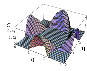
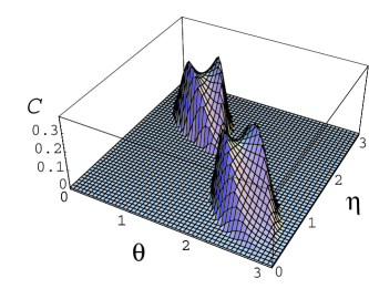
Figure 1: (Color online). The function ${\cal C}(\rho,\theta,0,\eta,0)$ for the $GHZ$-state (a) and for the $W$-state (b).

In Fig. 2 we show the function ${\cal I}^{(N)}(\rho)$ for three classes of mixed states: mixtures of $\left|GHZ\right\rangle$ and $\left|W\right\rangle$, mixtures of $\left|GHZ\right\rangle$ and the factorized state $\left|111\right\rangle$, and mixtures of $\left|W\right\rangle$ and $\left|111\right\rangle$. In this figure and in the next analogous ones, we plot the ratios between ${\cal I}^{(N)}(\rho)$ and ${\cal I}^{(N)}_{0}={\cal I}^{(N)}(\rho_{GHZ})$. It is well visible that ${\cal I}^{(1)}(\rho)$ and ${\cal I}^{(4)}(\rho)$ approach zero as the state approaches a factorized state, while these quantities reach higher values as the state possesses tripartite entanglement.

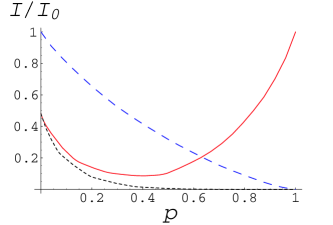
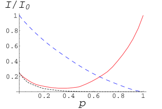
Figure 2: (Color online). The functions ${\cal I}^{(N)}(\rho)/{\cal I}^{(N)}_{0}$ for three exemplar mixed states. Figure (a) corresponds to $N=1$ and figure (b) to $N=4$. In both figures, the solid (red) line corresponds to the state $\rho=p\left|GHZ\right\rangle\left\langle GHZ\right|+(1-p)\left|W\right\rangle\left\langle W\right|$, the dotted (black) line to the state $\rho=p\left|111\right\rangle\left\langle 111\right|+(1-p)\left|W\right\rangle\left\langle W\right|$, and the dashed (blue) line to the state $\rho=p\left|111\right\rangle\left\langle 111\right|+(1-p)\left|GHZ\right\rangle\left\langle GHZ\right|$.

This analysis supports the idea that the criteria introduced in ref:Huber2010 are quite effective in revealing genuine tripartite entanglement. Nevertheless, it is important to note that the subset of trial states considered plays a very fundamental role in the detection of multipartite entanglement. Indeed, if we consider for example trial states of the form $|\tilde{\Psi}\rangle=\left|\theta,\phi\right\rangle\otimes\left|\theta,\phi\right\rangle\otimes\left|\eta,\xi\right\rangle\otimes\left|\eta,\xi\right\rangle\otimes\left|\eta,\xi\right\rangle\otimes\left|\theta,\phi\right\rangle$, then we are not able to detect entanglement of the GHZ-state. On the contrary, this choice is able to detect tripartite entanglement of the state $\left|\sigma GHZ\right\rangle=(\left|110\right\rangle+\left|001\right\rangle)/\sqrt{2}$, which instead never violates the inequality ${\cal Q}\leq 0$ when the trial state has the form given in (6). In fact, on the one hand, it is ${\cal I}^{(1)}(\rho_{\sigma GHZ})={\cal I}^{(4)}(\rho_{\sigma GHZ})=0$, while on the other hand, in Fig. 3 we can see that, when the trial state has the form $|\tilde{\Psi}\rangle$, it turns out to be ${\cal Q}>0$ in a wide range.

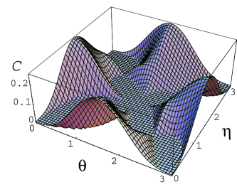
Figure 3: (Color online). The function ${\cal C}(\rho,\Psi)$ for the $GHZ$-like state $\left|\sigma GHZ\right\rangle=(\left|110\right\rangle+\left|001\right\rangle)/\sqrt{2}$ with the trial state $\left|\theta,0\right\rangle\otimes\left|\theta,0\right\rangle\otimes\left|\eta,0\right\rangle\otimes\left|\eta,0\right\rangle\otimes\left|\eta,0\right\rangle\otimes\left|\theta,0\right\rangle$.

In spite of these limitations related to spanning a subset of the relevant Hilbert space, we will use the functionals ${\cal I}^{(N)}(\rho)$ defined in (10) to carry on our analysis, both for the sake of simplicity and since we think it is effective enough in our problem.

III Thermal Tripartite Entanglement

Spin-star networks have been studied in connection with decoherence problems, especially in the analysis of the Non-Markovian character of spin baths ref:SSN-Decoherence , and for applications in quantum information ref:SSN-QuantumInfo .

In a recent paper, Wan-Li et al ref:Wan-Li2009 have studied the thermal entanglement in a spin-star system made of a central spin coupled to three peripheral spins through an anisotropic $\sigma$-$\sigma$ interactions (the longitudinal (‘$\sigma_{z}$-$\sigma_{z}$’) interaction and the total transverse interaction (‘$\sigma_{x}$-$\sigma_{x}$’$+$ ‘$\sigma_{y}$-$\sigma_{y}$’) have independent coupling strengths) identical for the three outer spins. More recently, a similar system has been studied, removing the longitudinal (i.e., $\sigma_{z}-\sigma_{z}$) interaction from the coupling between the spins, and introducing a certain inhomogeneity in the coupling strengths between the central spin and the outer ones ref:Anza2010 . Here we examine the same model, then considering the following Hamiltonian:

$$H=\frac{\omega_{0}}{2}\,\sum_{k=0}^{3}\,\hat{\sigma}_{z}^{k}\,+\,\sum_{k=1}^{3}\,c_{k}(\hat{\sigma}_{+}^{0}\hat{\sigma}_{-}^{k}+\hat{\sigma}_{-}^{0}\hat{\sigma}_{+}^{k})\,,$$ (12)

where $\hat{\sigma}_{\alpha}^{k}$ is the Pauli operator along the direction $\alpha$ ($\alpha=x,y,z$) of the spin $k$ ($k=0,1,2,3$), $\hat{\sigma}_{\pm}^{k}$ are the corresponding raising and lowering operators, $\omega_{0}$ is the free Bohr frequency of all the spins due to an external magnetic field, and $c_{k}$ is the coupling constant between the spin $0$ and the $k$-th one.

Once the system reaches the thermodynamical equilibrium, it can be described by the thermal state,

$$\rho^{(\mathrm{T})}=\frac{e^{-H/kT}}{\mathrm{tr}(e^{-H/kT})}\,\,,$$ (13)

which has the same eigenstates of the Hamiltonian $H$. The result of the diagonalization of $H$ is reported in the Appendix A.

In ref ref:Anza2010 , Anzà et al have considered the homogeneous case ($c_{1}=c_{2}=c_{3}=c$) and different kinds of inhomogeneous models. In the following we will consider both the homogeneous model and the inhomogeneous case $c_{1}=c_{3}=c$ and $c_{2}=c\,x$, with $x$ a dimensionless inhomogeneity parameter. We will apply the new criteria for multipartite entanglement detection to the state obtained starting from the four-qubit thermal state and tracing over the degrees of freedom of the central spin:

$$\rho^{(\mathrm{P})}=\mathrm{tr}_{0}(\rho^{(\mathrm{T})})\,\,,$$ (14)

which describes the three peripheral spins.

III.1 Homogeneous Model

The homogeneous model has been studied by Wan-Li et al ref:Wan-Li2009 (with the addition of a longitudinal coupling) and by Anzà et al ref:Anza2010 . In the first paper, the pairwise entanglement has been studied, through the use of concurrences. In the second paper, tripartite correlations have been investigated, through the use of the tripartite negativity ref:Sabin2008 .

Tripartite negativity is an imperfect tool to detect genuine tripartite entanglement, since it cannot distinguish between this form of entanglement and generalized biseparability. Nevertheless, it has helped to find points wherein tripartite correlations are significant, even if to disclose the nature of these correlations one needs a further analysis.

On the basis of the criteria proposed in ref ref:Huber2010 , it is possible to assert in an indisputable way the presence of tripartite entanglement when the condition ${\cal Q}>0$ is fulfilled. The quantity in (5) and its simplified version in (10), provide sufficient conditions for the presence of tripartite entanglement. Moreover, one could think that they furnish sorts of degree of entanglement, in the sense that higher values of these quantities can be understood as higher or wider violations of the inequality ${\cal Q}\leq 0$. Notwithstanding, it is important to stress that neither ${\cal I}^{(N)}$ nor ${\cal I}$ provide a measure of entanglement, and that in the case of ${\cal I}^{(N)}$ there is also the problem that a limited part of the relevant Hilbert space is spanned in the integration process, as already pointed out.

Fig. 4 and 5 show the tripartite negativity ${\cal N}(\rho^{(\mathrm{P})})$ and the quantity ${\cal I}^{(1)}(\rho^{(\mathrm{P})})$, respectively, as functions of both the temperature and the coupling constant between the central spin and the peripheral ones. Fig. 6 shows the quantities ${\cal I}^{(N)}(\rho^{(\mathrm{P})})$, for $N=1$ and $N=4$, as functions of the coupling constant, at low temperature. The behaviors are qualitatively very similar: for increasing temperature the quantity ${\cal I}^{(1)}(\rho^{(\mathrm{P})})$ decreases, while at very low temperature abrupt changes are well visible at specific values of the coupling constant. In particular, for $kT/\omega_{0}=0.01$, around the value of the coupling constant $c=0.6\omega_{0}$, there is a first transition from $0$ to a positive value, and around $c=3.7\omega_{0}$ another transition is well visible. These transitions, revealed by all the witness quantities here considered, correspond to very abrupt changes of the ground state of the four-qubit system. In particular, for $c<0.6\omega_{0}$ the ground state is $\left|\psi_{8}\right\rangle=\left|0000\right\rangle$, for $0.6\omega_{0}<c<3.7\omega_{0}$ the lowest energy state is $\left|\psi_{4}^{-}\right\rangle$, and for $c>3.7\omega_{0}$ the ground state is $\left|\psi_{2}^{-}\right\rangle$ (see Appendix A for the explicit expression of these states). The corresponding three-qubit states are: $\rho^{(\mathrm{P})}\approx\rho^{(8)}=\left|000\right\rangle\left\langle 000\right|$, $\rho^{(\mathrm{P})}\approx\rho^{(4-)}=0.5\,\left|111\right\rangle\left\langle 111\right|+0.5\,|\tilde{W}\rangle\langle\tilde{W}|$, and $\rho^{(\mathrm{P})}\approx\rho^{(2-)}=0.5\,|W\rangle\langle W|+0.5\,|\tilde{W}\rangle\langle\tilde{W}|$, respectively.

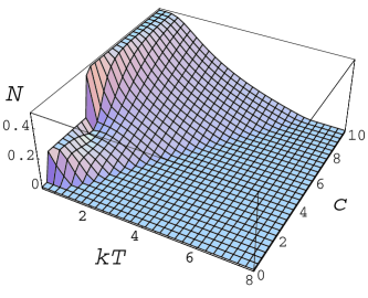
Figure 4: (Color online). The negativity for the state of the peripheral system ${\cal N}(\rho^{(\mathrm{P})})$ vs temperature ($kT$ in units of $\omega_{0}^{-1}$) and coupling constant ($c$ in units of $\omega_{0}^{-1}$).

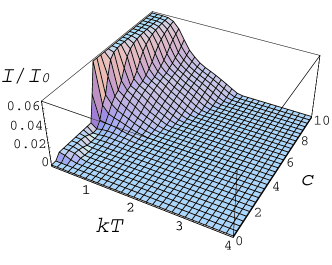
Figure 5: (Color online). The function ${\cal I}^{(1)}(\rho^{(\mathrm{P})})/{\cal I}^{(1)}_{0}$ for the state of the peripheral system vs temperature ($kT$ in units of $\omega_{0}^{-1}$) and coupling constant ($c$ in units of $\omega_{0}^{-1}$).

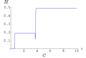
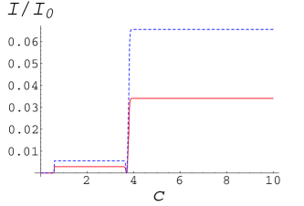
Figure 6: Figure (a) shows the low temperature profile of the tripartite negativity of the peripheral state ${\cal N}(\rho^{(\mathrm{P})})$ versus the coupling constant $c$ (in units of $\omega_{0}^{-1}$). Figure (b) shows the low temperature profiles of ${\cal I}^{(1)}(\rho^{(\mathrm{P})})/{\cal I}^{(1)}_{0}$ (solid curve, red online) and ${\cal I}^{(4)}(\rho^{(\mathrm{P})})/{\cal I}^{(4)}_{0}$ (dashed curve, blue online) . In both figures, the temperature is such that $kT/\omega_{0}=0.01$..

III.2 Inhomogeneous Model

In ref:Anza2010 , it has also been analyzed the effect of anisotropy in the coupling constants. The analysis based on the tripartite negativity shows that, in spite of the lack of symmetry of the system, the degree of correlation between the three peripheral spins can still be appreciable. In particular, it has been brought to the light the fact that at low temperature the maximum of tripartite negativity is reached for values of the inhomogeneity parameter different from (larger than) unity. Such behavior is well visible in Fig. 7 and Fig. 9a. This unexpected result seemingly suggests that the maximum of tripartite correlations does not correspond to the maximum of symmetry of the system.

It can be interesting to compare such results with those coming from the tools based on the work by Huber et al ref:Huber2010 . Fig. 8 shows the quantity ${\cal I}^{(1)}(\rho^{(\mathrm{P})})$ as a function of temperature and anisotropy parameter $x$, for $c=6\omega_{0}$. Fig. 9 shows the low temperature profiles, where fast transitions are very well visible. The local maximum of the tripartite negativity around $x=2.5$ is appreciable. On the contrary, the quantity ${\cal I}^{(4)}(\rho^{(\mathrm{P})})$ does not exhibit the same behavior. Instead, it does possess a maximum in $x=1$.

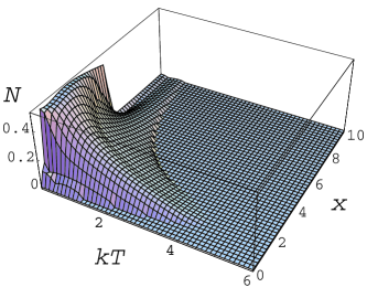
Figure 7: (Color online). The tripartite negativity of the peripheral state, ${\cal N}(\rho^{(\mathrm{P})})$, for the inhomogeneous model, as a function of both temperature ($kT$ in units of $\omega_{0}^{-1}$) and inhomogeneity parameter, with $c=6\omega_{0}$.

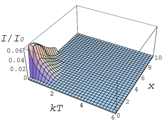
Figure 8: (Color online). The function ${\cal I}^{(1)}(\rho^{(\mathrm{P})})/{\cal I}^{(1)}_{0}$ for the thermalized system in the presence of inhomogeneity, for $c=6\omega_{0}$. This quantity is plotted versus the temperature ($kT$ in units of $\omega_{0}^{-1}$) and the inhomogeneity parameter $x$.

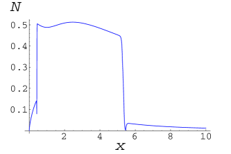
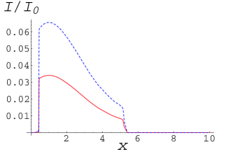
Figure 9: (Color online). Figure (a) shows the low temperature profile of the tripartite negativity of the peripheral state ${\cal N}(\rho^{(\mathrm{P})})$ versus the inhomogeneity parameter $x$. Figure (b) shows the low temperature profiles of ${\cal I}^{(1)}(\rho^{(\mathrm{P})})/{\cal I}^{(1)}_{0}$ (solid curve, red online) and ${\cal I}^{(4)}(\rho^{(\mathrm{P})})/{\cal I}^{(4)}_{0}$ (dashed curve, blue online) . In both figures, the coupling constant is $c=6\omega_{0}$ and the temperature is such that $kT/\omega_{0}=0.01$.

At low temperature, both ${\cal N}(\rho^{(\mathrm{P})})$ and the ${\cal I}^{(N)}$ functionals have significant values for intermediate values of $x$, say for $0.5\lesssim x\lesssim 5$, and are small or vanishing out of this region. Note that for very small $x$ ($c_{2}\ll c_{1},c_{3}$) one of the spins is almost uncoupled to the central one. On the other hand, for large $x$ ($c_{2}\gg c_{1},c_{3}$) that spin has a much stronger coupling constant than the other two, whose couplings can then be considered as a perturbation, so that, at zeroth order, the latter two spins are uncoupled to the central one. In both cases, it is physically reasonable that tripartite correlations between the outer spins are negligible or absent. The abrupt changes of the witness quantities are related to the sudden modifications of the ground state of the system. However, we remark that low or vanishing values of the tripartite negativity and ${\cal I}^{(N)}$ (or even ${\cal I}$) do not guarantee the absence of tripartite entanglement or tripartite correlations. Conversely, the non-vanishing values of some ${\cal I}^{(N)}$ functionals guarantee the presence of tripartite entanglement.

IV Discussion

In this paper we have investigated the tripartite thermal entanglement in a spin-star network with three peripheral spins. The interaction with the central spin is responsible for the establishment of tripartite correlations between the peripheral ones, and such correlations survive even when the system is at thermal equilibrium. We have considered both the homogeneous model, where all the coupling constants are equal, and the inhomogeneous model, where one of the outer spins is coupled to the central one with a different strength.

The analysis is carried on through the use of the quantities defined in (10), which is a simplified version of (5), where a limited region of the relevant Hilbert space is spanned. Each of these functionals has the property that its strict positivity guarantees the presence of genuine tripartite entanglement. Nevertheless, it must be clarified that none of such quantities provides a measure of the amount of tripartite entanglement. Anyway, a larger value of ${\cal I}$ does mean a higher or wider violations of the condition ${\cal Q}\leq 0$. Therefore, one can conjecture that a higher value of ${\cal I}$ corresponds to a state that exhibits entanglement more than other states. The same assertion is weaker when applied to ${\cal I}^{(N)}$, since evaluation of this functional does not require spanning over all of the Hilbert space. Moreover, it is important to know that the use of different ${\cal I}$-functionals (${\cal I}$, ${\cal I}^{(N)}$ with different $N$, or other similar quantities that consider spanning on different subsets of the relevant Hilbert space) could lead to different predictions.

For the homogeneous model, the low temperature behavior is characterized by abrupt changes of the quantities ${\cal I}^{(N)}$ versus the coupling constant. These transitions correspond to concomitant abrupt changes of the system ground state. At higher temperature, ${\cal I}^{(1)}$ goes to zero. For the inhomogeneous model, the dependence of ${\cal I}^{(1)}$ on the inhomogeneity parameter and temperature, when the coupling constant is fixed at some high value, is again characterized by abrupt changes with respect to $x$ at low temperature, and by vanishing at high temperature. It is remarkable that, at low temperature, the dependence on the inhomogeneity parameter reveals the presence of a maximum for $x=1$, i.e. in the homogeneous case. This result, on the one hand is seemingly in line with expectations coming from intuition, and on the other hand is supposedly different from the predictions coming from the use of tripartite negativity. Nevertheless, different behaviors of these quantities do not imply contradictions, since neither tripartite negativity nor the ${\cal I}$-quantities provide necessary conditions for the presence of tripartite entanglement or a measure of such form of entanglement. What is sure is that in the parameter region where ${\cal I}^{(N)}$ is non vanishing, the thermal state possesses genuine tripartite entanglement.

Therefore, in spite of the limitations of our analysis, we have found genuine tripartite entanglement in our system at thermal equilibrium, even at non vanishing temperature and in the presence of inhomogeneity.

Appendix A Diagonalization of $H$

In this appendix we give eigenvalues and eigenvectors of the Hamiltonian in (12), as functions of $x$, $c>0$ and $\omega_{0}$. The homogeneous model is obtained for $x=1$.

The eigenvalues of the Hamiltonian are:

$$E_{1}^{\pm} = \pm c\,,$$ (15a)

$$E_{2}^{\pm} = \pm\frac{c}{2}\left[x+\left(8+x^{2}\right)^{\frac{1}{2}}\right]\,,$$ (15b)

$$E_{3}^{\pm} = \pm\frac{c}{2}\left[x-\left(8+x^{2}\right)^{\frac{1}{2}}\right]\,,$$ (15c)

$$E_{4}^{\pm} = \pm\left[c\left(2+x^{2}\right)^{\frac{1}{2}}+\omega_{0}\right]\,,$$ (15d)

$$E_{5}^{\pm} = \pm\left[c\left(2+x^{2}\right)^{\frac{1}{2}}-\omega_{0}\right]\,,$$ (15e)

$$E_{6} = -\omega_{0}\,,$$ (15f)

$$E_{7} = \omega_{0}\,,$$ (15g)

$$E_{8} = -2\omega_{0}\,,$$ (15h)

$$E_{9} = 2\omega_{0}\,,$$ (15i)

where the eigenvalues $E_{6}$ and $E_{7}$ are twofold degenerate eigenvalues.

The relevant eigenstates are:

$$\left|\psi_{1}^{\pm}\right\rangle = \frac{1}{2}\left[\left(\left|0011\right\rangle\pm\left|1100\right\rangle\right)-\left(\left|0110\right\rangle\pm\left|1001\right\rangle\right)\right]\,,$$

(16a)

$$\left|\psi_{2}^{\pm}\right\rangle = \frac{1}{K_{1}}\>[\left(\left|0011\right\rangle\pm\left|1100\right\rangle\right)+\left(\left|0110\right\rangle\pm\left|1001\right\rangle\right)$$ (16b)

$$+ \frac{\sqrt{8+x^{2}}-x}{2}\left(\left|0101\right\rangle\pm\left|1010\right\rangle\right)]\,,$$

$$\left|\psi_{3}^{\pm}\right\rangle = \frac{1}{K_{1}}\>[\left(\left|0011\right\rangle\pm\left|1100\right\rangle\right)+\left(\left|0110\right\rangle\pm\left|1001\right\rangle\right)$$ (16c)

$$- \frac{\sqrt{8+x^{2}}+x}{2}\left(\left|0101\right\rangle\pm\left|1010\right\rangle\right)]\,,$$

$$\left|\psi_{4}^{\pm}\right\rangle = \frac{1}{K_{2}}\left[\sqrt{2+x^{2}}\left|0111\right\rangle\right.$$ (16d)

$$\pm \left.\left(\left|1011\right\rangle+x\left|1101\right\rangle+\left|1110\right\rangle\right)\right]\,,$$

$$\left|\psi_{5}^{\pm}\right\rangle = \frac{1}{K_{2}}\left[\left(\left|0100\right\rangle+x\left|0010\right\rangle+\left|0001\right\rangle\right)\right.$$ (16e)

$$\pm \left.\sqrt{\left(2+x^{2}\right)}\left|1000\right\rangle\right]\,,$$

$$\left|\psi_{6}^{\alpha}\right\rangle = \frac{1}{K_{3}}\left[\frac{1}{x}\left|0001\right\rangle+\left|0010\right\rangle-\left(\frac{1}{x}+x\right)\left|0100\right\rangle\right]\,,$$

$$\left|\psi_{6}^{\beta}\right\rangle = \frac{1}{\sqrt{1+x^{2}}}\left(\left|0010\right\rangle-x\left|0001\right\rangle\right)\,,$$ (16f)

$$\left|\psi_{7}^{\alpha}\right\rangle = \frac{1}{K_{3}}\left[\frac{1}{x}\left|1011\right\rangle+\left|1101\right\rangle-\left(\frac{1}{x}+x\right)\left|1110\right\rangle\right]\,,$$

$$\left|\psi_{7}^{\beta}\right\rangle = \frac{1}{\sqrt{1+x^{2}}}\left(\left|1101\right\rangle-x\left|1011\right\rangle\right)\,,$$ (16g)

$$\left|\psi_{8}\right\rangle = \left|0000\right\rangle\,,$$ (16h)

$$\left|\psi_{9}\right\rangle = \left|1111\right\rangle\,,$$ (16i)

with

$${K_{1}}^{2}=4+2\left(\frac{\sqrt{8+x^{2}}-x}{2}\right)^{2}\,,$$ (17a)

$${K_{2}}^{2}=2\left(2+x^{2}\right)\,,$$ (17b)

$${K_{3}}^{2}=\frac{2}{x^{2}}+3+x^{2}\,.$$ (17c)

References

- (1) A. Peres, Phys. Rev. Lett. 77, 1413 (1996); K. Zyczkowski, P. Horodecki, A. Sanpera, M. Lewenstein, Phys. Rev. A 58, 883 (1998); G. Vidal, R. F. Werner, Phys. Rev. A 65, 032314 (2002).
- (2) W. K. Wootters, Phys. Rev. Lett. 80, 2245 (1998).
- (3) V. Coffman, J. Kundu, W. K. Wootters, Phys. Rev. A 61, 052306 (2000).
- (4) A. Wong and N. Christensen, Phys. Rev. A 63, 044301 (2001).
- (5) D. A. Meyer and N. R. Wallach, J. Math. Phys. 43, 4273 (2002).
- (6) P. Facchi, G. Florio, U. Marzolino, G. Parisi and S. Pascazio, J. Phys. A: Math. Theor. 42, 055304 (2009).
- (7) Lin Chen and Yi-Xin Chen, Phys. Rev. A 76, 022330 (2007).
- (8) M. Wiesiak, V. Vedral, C. Brukner, New J. Phys. 7, 258 (2005).
- (9) G. S. L. Brandão Fernando, Phys. Rev. A 72, 022310 (2005).
- (10) For a review on entanglement in multipartite systems, see: L. Amico, R. Fazio, A. Osterloh and V. Vedral, Rev. Mod. Phys. 80, 517 (2008).
- (11) E. Jung, D. Park, J. W. Son, Phys. Rev. A 80, 010301(R) (2009).
- (12) C. Sabin and G. Garcia-Alcaine, Eur. Phys. J. D 48, 435 (2008).
- (13) M. Huber, F. Mintert, A. Gabriel and B. C. Hiesmayr, Phys. Rev. Lett. 104, 210501 (2010).
- (14) M. C. Arnesen, S. Bose, V. Vedral, Phys. Rev. Lett. 87, 017901 (2001).
- (15) A. Osterloh et al, Nature 416, 608 (2002).
- (16) T. J. Osborne and M. A. Nielsen, Phys. Rev. A 66, 032110 (2002)
- (17) Shou-Shu Gong and Gang Su, Phys. Rev. A 80, 012323 (2009).
- (18) Hao Wang, Sanqiu Liu, and Jizhou He, Phys. Rev. E 79, 041113 (2009).
- (19) Amit Kumar Pal and Indrani Bose, J. Phys.: Cond. Matt. 22, 016004 (2010).
- (20) Yue Zhou et al, Europhys. Lett. 86, 50004 (2009).
- (21) T. Werlang and G. Rigolin Phys. Rev. A 81, 044101 (2010).
- (22) A. M. Souza et al, Phys. Rev. B 79, 054408 (2009).
- (23) A. Hutton and S. Bose, Phys. Rev. A 69, 042312 (2004).
- (24) Y. Wan-Li, W. Hua, F. Mang, and A. Jun-Hong, Chinese Phys. B 18, 3677 (2009).
- (25) F. Anzà, B. Militello and A. Messina, J. Phys. B 43, 205501 (2010).
- (26) H.-P. Breuer, D. Burgarth, and F. Petruccione, Phys. Rev. B 70, 045323 (2004); H. Krovi, O. Oreshkov, M. Ryazanov, and D. A. Lidar, Phys. Rev. A 76, 052117 (2007); E. Ferraro, H.-P. Breuer, A. Napoli, M. A. Jivulescu, and A. Messina, Phys. Rev. B 78, 064309 (2008); D. Rossini, P. Facchi, R. Fazio, G. Florio, D. A. Lidar, S. Pascazio, F. Plastina, and P. Zanardi, Phys. Rev. A 77, 052112 (2008).
- (27) N. Arshed, A. H. Toor, and D. A. Lidar, Phys. Rev. A 81, 062353 (2010); Yuhan Chen et al, Phys. Rev. A 81, 032338 (2010).