Statistical Properties of Ideal Ensemble of Disordered 1$D$ Steric Spin-Chains

Abstract

The statistical properties of ensemble of disordered 1$D$ steric spin-chains (SSC) of various length are investigated. Using 1$D$ spin-glass type classical Hamiltonian, the recurrent trigonometrical equations for stationary points and corresponding conditions for the construction of stable 1$D$ SSCs are found. The ideal ensemble of spin-chains is analyzed and the latent interconnections between random angles and interaction constants for each set of three nearest-neighboring spins are found. It is analytically proved and by numerical calculation is shown that the interaction constant satisfies Lev́y’s alpha-stable distribution law. Energy distribution in ensemble is calculated depending on different conditions of possible polarization of spin-chains. It is specifically shown that the dimensional effects in the form of set of local maximums in the energy distribution arise when the number of spin-chains $M<<N^{2}_{x}$ (where $N_{x}$ is number of spins in a chain) while in the case when $M\propto N^{2}_{x}$ energy distribution has one global maximum and ensemble of spin-chains satisfies Birkhoff’s ergodic theorem. Effective algorithm for parallel simulation of problem which includes calculation of different statistic parameters of 1$D$ SSCs ensemble is elaborated.

I Formulation of the problem

Let us consider classical ensemble of disordered 1$D$ steric spin-chains (SSC), where it is supposed that interactions between spin-chains are absent (later it will be called an ideal ensemble) and that there are $N_{x}$ spins in an each chain. Despite some ideality of the model it can be interesting enough and rather convenient for investigation of a number of important and difficult applied problems of physics, chemistry, material science, biology, evolution, organization dynamics, hard-optimization, environmental and social structures, human logic systems, financial mathematics etc (see for example Young ; Bov ; Fisch ; Tu ; Chary ; Baake ). As was shown by authors spin-glass model can be used for investigation of media’s properties on scales of space-time periods of an external fields at conditions far from a usual equilibrium of media gev .

Mathematically mentioned type of ideal ensemble can be generated by 1$D$ Heisenberg spin-glass Hamiltonian without external field Bind ; Mezard ; Young :

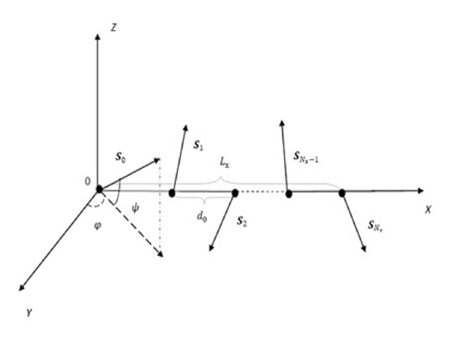
Figure 1: A stable $1D$ steric spin-chain with random interactions and the length of $L_{x}$. The spherical angles $\varphi$ and $\psi$ describe the spatial orientation of $\textbf{\emph{S}}_{0}$ spin, the pair of angles $(\varphi_{i},\psi_{i})$ correspondingly defines the spatial orientation of the spin $\textbf{\emph{S}}_{i}$, the distance between two neighboring spins in $1D$ lattice is $d_{0}$.

$$H_{0}(N_{x})=-\sum_{i=0}^{N_{x}-1}J_{i\,i+1}{\textbf{\emph{S}}}_{i}{\textbf{\emph{S}}}_{i+1}.$$ (1)

where ${\textbf{\emph{S}}}_{i}$ describes the $i$-th spin which is a unit length vector and has a random orientation. In the expression (1) $J_{i\,i+1}$ characterizes a random interaction constant between $i$ and $i+1$ spins, which can have positive and negative values as well EdwAnd .

In other words we consider the mathematical model of spin-chains ensemble where every spin-chain is like a regular 1$D$ lattice with the length $L_{x}=d_{0}N_{x}$, where spins are put on nodes of lattice and interactions between them are random (see FIG 1).

The distribution of spin-spin interaction constant $W(J)$ is chosen from considerations of convenience and as a rule it is a Gauss-Edwards-Anderson model EdwAnd (see also Bind ):

$$W(J)=\frac{1}{\sqrt{2\pi(\Delta{J})^{2}}}\exp\biggl{\{}-\frac{\bigl{(}J-J_{0}\bigr{)}^{2}}{2(\Delta{J})^{2}}\biggr{\}},$$ (2)

where $J_{0}=\bigl{<}J\bigr{>}_{av}$ and $\bigl{(}\Delta{J}\bigr{)}^{2}=\bigl{<}J^{2}\bigr{>}_{av}-\bigl{<}J\bigr{>}_{av}^{2}$.

Let us recall that $J_{0}$ and $\Delta{J}$ for this model are independent from the distance and scaled with the spin number $N_{x}$ as:

$$\bigl{<}J\bigr{>}_{av}=J_{0}\propto{N_{x}^{-1}},\qquad\Delta{J}\propto{N_{x}^{-1/2}},$$ (3)

in order to ensure a sensible thermodynamic limit. $\bigl{<}...\bigr{>}_{av}$ in Eqs. (2) and (3) describes the averaging procedure. Below we will investigate the issue of how much lawful the choice of this model is.

For further investigations it is useful to rewrite the Hamiltonian (1) in spherical coordinates (see FIG 1):

$$H_{0}(N_{x})=-\sum_{i=0}^{N_{x}-1}J_{i\,i+1}\bigl{[}\cos\psi_{i}\cos\psi_{i+1}\cos(\varphi_{i}-\varphi_{i+1})+\sin\psi_{i}\sin\psi_{i+1}\bigr{]}.$$ (4)

A stationary point of the Hamiltonian is given by the system of trigonometrical equations:

$$\frac{\partial{H_{0}}}{\,\,\partial\psi_{i}}=0,\qquad\qquad\frac{\partial{H_{0}}}{\,\,\partial\varphi_{i}}=0,$$ (5)

where ${\Theta}_{i}=(\psi_{i},\varphi_{i})$ are angles of $i$-th spin in the spherical coordinates system ($\psi_{i}$ is a polar and $\varphi_{i}$ is an azimuthal angles), $\mathbf{\Theta}=({\Theta_{1}},{\Theta_{2}}....{\Theta_{N_{x}}})$ respectively describe the angular part of a spin-chain configuration.

Now using expression (4) and equations (5) it is easy to find the following system of trigonometrical equations:

$$\sum_{\nu=i-1;\,\,\nu\neq i}^{i+1}J_{\nu i}\bigl{[}\sin\psi_{\nu}-\tan\psi_{i}\cos\psi_{\nu}\cos(\varphi_{i}-\varphi_{\nu})\bigr{]}=0,$$

$$\sum_{\nu=i-1;\,\,\nu\neq i}^{i+1}J_{\nu i}\,\cos\psi_{\nu}\sin(\varphi_{i}-\varphi_{\nu})=0,\,\,\,\qquad\,J_{\nu i}\equiv J_{i\nu}.$$ (6)

In case when all the interaction constants between $i$-th spin with its nearest-neighboring spins $J_{i-1\,i}$,   $J_{i\,i+1}$ and angle configurations $\bigl{(}\psi_{i-1},\varphi_{i-1}\bigr{)}$,  $\bigl{(}\psi_{i},\varphi_{i}\bigr{)}$ are known, it is possible to explicitly calculate the pair of angles ${\Theta_{i+1}}=\bigl{(}\psi_{i+1},\varphi_{i+1}\bigr{)}$. Correspondingly, the $i$-th spin will be in the ground state (in the state of minimum energy) if in the stationary point ${\Theta_{i}^{0}}=\bigl{(}\psi_{i}^{0},\varphi_{i}^{0}\bigr{)}$ the following conditions are satisfied:

$$A_{\psi_{i}\psi_{i}}({\Theta_{i}^{0}})>0,\qquad A_{\psi_{i}\psi_{i}}({\Theta_{i}^{0}})\,A_{\varphi_{i}\varphi_{i}}({\Theta_{i}^{0}})-A_{\psi_{i}\phi_{i}}^{2}({\Theta_{i}^{0}})>0,$$ (7)

where $A_{\alpha_{i}\alpha_{i}}({\Theta_{i}^{0}})={\partial^{2}{H_{0}}}/{\partial\alpha_{i}^{2}},\quad A_{\alpha_{i}\beta_{i}}({\Theta_{i}^{0}})=A_{\beta_{i}\alpha_{i}}({\Theta_{i}^{0}})={\partial^{2}{H_{0}}}/{\partial\alpha_{i}\partial\beta_{i}}$, in addition:

$$A_{\psi_{i}\psi_{i}}({\Theta_{i}^{0}})\,=\,\biggl{\{}\,\sum_{\nu=i-1;\,\,\nu\neq i}^{i+1}J_{\nu i}\bigl{[}\cos\psi_{\nu}\cos(\varphi_{\nu}-\varphi_{i}^{0})+\tan\psi_{i}^{0}\sin\psi_{\nu}\bigr{]}\biggr{\}}\cos\psi_{i}^{0},\,\,\,\,$$

$$A_{\varphi_{i}\varphi_{i}}({\Theta_{i}^{0}})=\biggl{\{}\,\sum_{\nu=i-1;\,\,\nu\neq i}^{i+1}J_{\nu i}\cos\psi_{\nu}\cos(\varphi_{\nu}-\varphi_{i}^{0})\biggr{\}}\cos\psi_{i}^{0},\qquad\qquad\qquad$$

$$A_{\psi_{i}\phi_{i}}({\Theta_{i}^{0}})=\biggl{\{}\,\sum_{\nu=i-1;\,\,\nu\neq i}^{i+1}J_{\nu i}\cos\psi_{\nu}\sin(\varphi_{\nu}-\varphi_{i}^{0})\,\biggr{\}}\sin\psi_{i}^{0}.\qquad\qquad\qquad$$ (8)

Taking into account the second equation in (6) we can reduce condition (7) to the following kind:

$$A_{\psi_{i}\psi_{i}}({\Theta_{i}^{0}})>0,\qquad\qquad A_{\varphi_{i}\varphi_{i}}({\Theta_{i}^{0}})>0.$$ (9)

So, with the help of Eq.s (6) and conditions (9) huge number of stable $1D$ SSCs may be calculated and on its basis it is possible to further construct the statistical properties of 1$D$ SSCs ensemble. It is important to note that the average polarization of 1$D$ SSCs ensemble is supposed to be equal to zero.

Now we can construct the distribution function of energy in 1$D$ SCCs ensemble. To this effect it is useful to divide the nondimensional energy axis $\varepsilon=\epsilon/\delta\epsilon$ into regions $0>\varepsilon_{0}>...>\varepsilon_{n}$, where $n>>1$ and $\epsilon$ is a real energy axis. The number of stable 1$D$ SSC configurations with length of $L_{x}$ in the range of energy $[\varepsilon-\delta\varepsilon,\varepsilon+\delta\varepsilon]$ will be denoted by $M_{L_{x}}(\varepsilon)$ while the number of all stable 1$D$ SSC configurations - correspondingly by symbol $M_{L_{x}}^{full}=\sum_{j=1}^{n}M_{L_{x}}(\varepsilon_{j})$. Accordingly, the energy distribution function into the 1$D$ SSCs ensemble may be defined by expressions:

$$F_{L_{x}}(\varepsilon;d_{0}(T))=M_{L_{x}}(\varepsilon)/M_{L_{x}}^{full},$$ (10)

where distribution function is normalized to unit:

$$\lim_{n\to\infty}\sum^{n}_{j=1}F_{L_{x}}(\varepsilon_{j};d_{0}(T))\delta\varepsilon_{j}=\int^{\,0}_{-\infty}F_{L_{x}}(\varepsilon;d_{0}(T))d\varepsilon=1.$$

By similar way we can define also distributions for polarization and for a spin-spin interaction constant.

II Algorithm of 1$D$ SSCs Ideal Ensemble Simulation

Now our aim is elaboration of algorithm for parallel simulation of ideal ensemble of $1D$ SSCs.
Using equations (6) for stationary points of Hamiltonian $H_{0}(N_{x})$ we can find the following equations system:

$$J_{i-1\,i}\bigl{[}\sin\psi_{i-1}-\tan\psi_{i}\cos\psi_{i-1}\cos(\varphi_{i}-\varphi_{i-1})\bigr{]}+J_{i\,i+1}\bigl{[}\sin\psi_{i+1}$$

$$-\tan\psi_{i}\cos\psi_{i+1}\cos(\varphi_{i}-\varphi_{i+1})\bigr{]}=0,$$

$$J_{i-1\,i}\,\cos\psi_{i-1}\sin(\varphi_{i}-\varphi_{i-1})\,+J_{i+1\,i}\,\cos\psi_{i+1}\sin(\varphi_{i}-\varphi_{i+1})=0.$$ (11)

After designations:

$$x=\cos\psi_{i+1},\qquad y=\sin(\varphi_{i}-\varphi_{i+1}),$$ (12)

the system (11) may be transformed to the following form:

$$C_{1}+J_{i\,i+1}\bigl{[}\sqrt{1-x^{2}}-\tan\psi_{i}\,x\sqrt{1-y^{2}}\bigr{]}=0,\qquad C_{2}+J_{i\,i+1}\,x\,y=0,$$ (13)

where parameters $C_{1}$ and $C_{2}$ are defined by expressions:

$$C_{1}=J_{i-1\,i}\bigl{[}\sin\psi_{i-1}-\tan\psi_{i}\cos\psi_{i-1}\cos(\varphi_{i}-\varphi_{i-1})\bigr{]},$$

$$C_{2}=J_{i-1\,i}\cos\psi_{i-1}\sin(\varphi_{i}-\varphi_{i-1}).\qquad\qquad\qquad\qquad\,\,$$ (14)

From the system of equations (13) we can find the equation for the unknown variable $y$:

$$C_{1}y+C_{2}\sqrt{1-y^{2}}\tan\psi_{i}+\sqrt{J_{i\,i+1}^{2}y^{2}-C_{2}^{2}}=0.$$ (15)

We can transform the equation (15) to the following equation of fourth order:

$$\bigl{[}A^{2}+4C_{1}^{2}C_{2}^{2}\sin\psi_{i}\bigl{]}y^{4}-2\bigl{[}AC_{2}^{2}+2C_{1}C_{2}^{2}\sin^{2}\psi_{i}\bigr{]}y^{2}+C_{2}^{4}=0,$$ (16)

where

$$A=J^{2}_{i\,i+1}\cos^{2}\psi_{i}-C_{1}^{2}+C_{2}^{2}\sin^{2}\psi_{i}.$$ (17)

Discriminant of equation (16) is equal to:

$$D=C_{2}^{4}\bigl{(}A+2C_{1}\sin^{2}\psi_{i}\bigr{)}^{2}-C_{2}^{4}\bigl{(}A^{2}+4C_{1}^{2}C_{2}^{2}\sin^{2}\psi_{i}\bigr{)}$$

$$=4C^{4}_{2}C^{2}_{1}\sin^{2}\psi_{i}\bigl{(}A+C^{2}_{1}\sin^{2}\psi_{i}-C^{2}_{2}).\qquad\qquad$$

From the condition of nonnegativity of discriminant $D\geq 0$ we can find the following condition:

$$A+C^{2}_{1}\sin^{2}\psi_{i}-C^{2}_{2}\geq 0.$$ (18)

Further substituting the value of $A$ from (17) into (18) we can find the new condition to which the interaction constant between two successive spins should satisfy:

$$J_{i\,i+1}^{2}\geq C^{2}_{1}+C^{2}_{2}.$$ (19)

Now we can write the following expressions for unknown variables $x$ and $y$:

$$x^{2} =\frac{C_{2}^{2}}{J_{i\,i+1}^{2}y^{2}},$$

$$y^{2} =C_{2}^{2}\,\frac{\cos^{2}\psi_{i}J_{i\,i+1}^{2}\pm 2C_{1}\sin\psi_{i}\cos\psi_{i}\sqrt{J_{i\,i+1}^{2}-C_{1}^{2}-C_{2}^{2}}+C_{3}+2C_{1}^{2}\sin^{2}\psi_{i}}{\cos^{4}\psi_{i}J_{i\,i+1}^{4}+2C_{3}\cos^{2}\psi_{i}J_{i\,i+1}^{2}+(C_{1}^{2}+\sin^{2}\psi_{i}C_{2}^{2})^{2}},$$ (20)

where $C_{3}=-C_{1}^{2}+C_{2}^{2}\,\sin^{2}\psi_{i}.$
Finally taking into account designations (12) we can find new conditions of restriction of the calculated angles $\bigl{(}\varphi_{i+1},\psi_{i+1}\bigr{)}$:

$$0\leq x^{2}\leq 1,\qquad 0\leq y^{2}\leq 1.$$ (21)

These conditions are very important for elaborating correct and effective algorithm for numerical simulations.

II.1 Algorithm description

This is parallel algorithm for simulation of 1$D$ SSCs ensemble, which consists of separate iterative calculations of nodes in 1$D$ SSC. The first and second nodes are initialized randomly, then $i$-th node is obtained from $(i-2)$-th and $(i-1)$-th layers nodes. Every node contains the following information:
$\varphi$-polar angle,
$\psi$-azimuthal angle,
$J$-interaction coefficient,

The following parameters are initializes in the following way:
$\varphi_{0}$ and $\varphi_{1}$ - rand()${}^{\ast}2^{\ast}\pi^{\ast}R$;
$\psi_{0}$ and $\psi_{1}$ - acos (rand());
$J_{0\,1}$ - rand();

where rand() function generates uniformly distributed random numbers on the interval $(0,1)$.

The algorithm pseudo-code is following:

// generate $n$ separate independent sets of problem in parallel

for $i=1:N_{x}$

for $j=1:R$  // regenerate $J_{i}$ maximum $R$ times if needed

for $k=1:L_{i}$  // go through all elements in the $i$-th layer if conditions

// (9) are satisfied

begin

// calculate energy on $i$-th layer,

// calculate polarization on $x,y$ and $z$-axis

// calculate $x_{i+1}$ and $y_{i+1},$

// save $J_{i}$ value

. . . .

end

endfor

endfor

endfor

if ($i==N_{x}$) // reached the $N_{x}$-th layer

begin

// save energy, polarizations values

end

endif
// construct distribution functions of energy $\varepsilon$, polarization $p$ and
// interaction constant $J$

// calculate the mean value of energy $\bar{\varepsilon}$, polarization $\bar{p}$, interaction constant $\bar{J}$ and
// its variance $\bar{J^{2}}$.

III Numerical Simulation

We will consider an ideal ensemble of 1$D$ SSCs which consists of $M$ number of spin-chains each of them with the length 25$d_{0}$. For realization of parallel simulation we will use algorithm A (see FIG 2).

The parallel algorithm works in the following way. Randomly $M$ sets of initial parameters are generated and parallel calculations of equations (20) for unknown variables $x$ and $y$ transact with taking into account conditions (21). However only specifying of initial conditions is not enough for solution of these equations. Evidently these equations can be solved after definition of the constant $J_{0\,1}$, which is also randomly generated. In the case when solutions are found then conditions of stability of spin in node (9) are checked. The solution proceeds for the following spin if the specified conditions (9) are satisfied. If conditions are not satisfied, a new constant $J_{0\,1}$ is randomly generated and correspondingly new solutions are found which are checked later on conditions (9). This cycle on each spin repeats until the solutions do not satisfy to conditions of the minimum spin energy in the node.

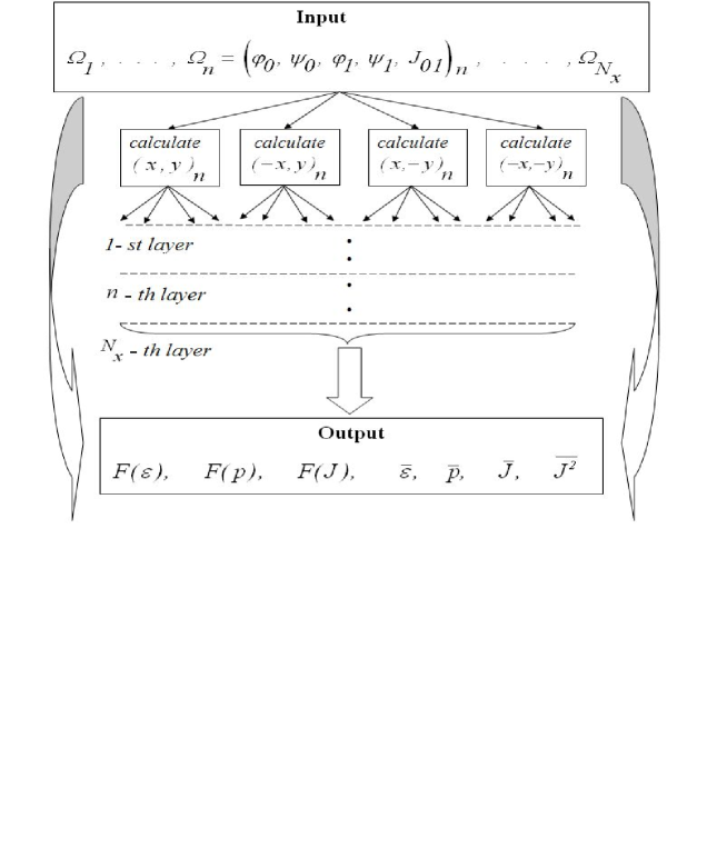
Figure 2: The algorithm of $1D$ SSCs of ideal ensemble parallel simulation of statistical parameters.

At first we have conducted numerical simulation for definition of different statistical parameters of the ensemble which consists of $10^{2}$ spin-chains. Let us recall that the number of simulation of spin-chains define the number of spin-chains in the ensemble. As the simulation shows (see the left picture in FIG 3) the energy distribution function has a set of local maximums ($\varepsilon^{(0)},...,\varepsilon^{(m)})$. Obviously they are dimensional effects and are similar to the first-order phase transitions which often happen in spin-glass systems Bind ).

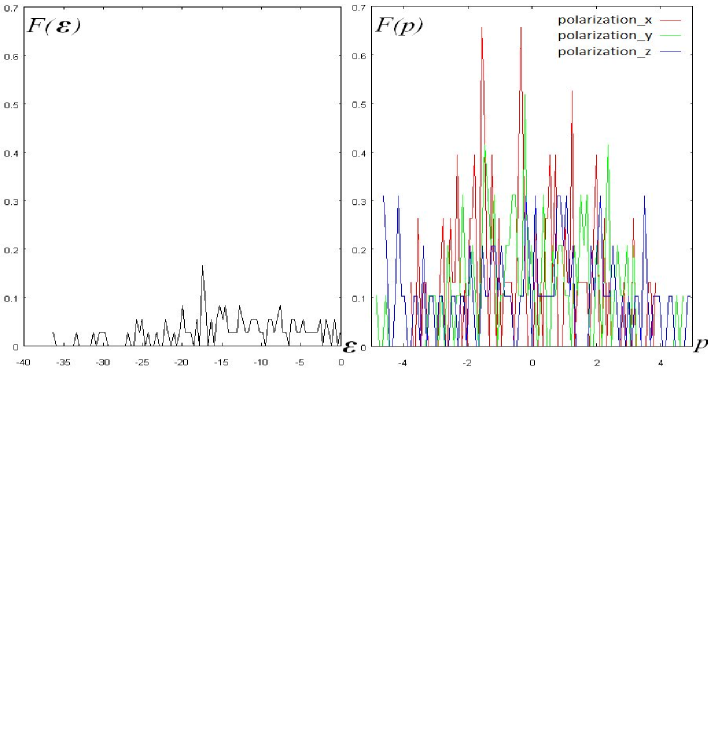
Figure 3: The energy distribution where there are apparently many local minimum of energy for ensemble of 1$D$ SSCs with the length of $L_{x}=25d_{0}$, which consists of $10^{2}$ spin-chains (the left picture). On the right picture polarization distributions of ensemble on coordinates $x,y$ and $z$ are shown.

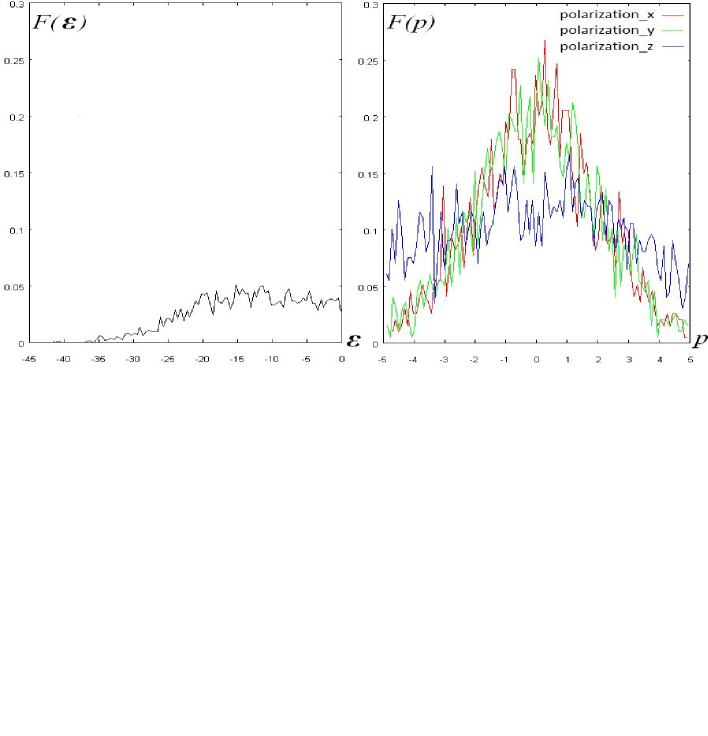
Figure 4: In the left picture is shown the energy distribution in the ensemble of 1$D$ SSCs with the length of $L_{x}=25d_{0}$, which consists of 2$\cdot 10^{3}$ spin-chains. Apparently, the number of local minimums of energy is promptly reduced comparing with the increase of spin-chains. On the right picture polarization distributions of ensemble on coordinates $x,y$ and $z$ are shown.

Let us note that during simulation we suppose that spin-chains can be polarized up to 20 percent i.e. the total value of spins sum in each chain can be in an interval of $-5\leq p\leq 5$, where $p$ designates the polarization of spin-chain. In other words each spin-chain is a vector of certain length which is directed to coordinate $x$. As calculations show, in the ensemble consisting of a small number of spin-chains, for example, of the order $10^{2}$, the self-averaging of spin-chains does not occur in full measure i.e. the total polarization of an ensemble differs from zero: $p_{x}=-0.33099,\,p_{y}=-0.035191,\,p_{z}=-0.024543$ where $p=\int_{-\infty}^{+\infty}F(p)dp$, where it is supposed that $p=(p_{x},\,p_{y},\,p_{z})$. In this case the average energy of an ensemble is equal to $\bar{\varepsilon}=-14.121$, where $\bar{\varepsilon}=\int_{-\infty}^{0}F(\varepsilon)\varepsilon d\varepsilon$.

For the ensemble which consists of $2.10^{3}$ spin-chains (see FIG 4), the dimensional effects practically disappear. The summary polarization of ensemble in this case is very small: $p_{x}=-0.020538,\,p_{y}=-0.047634,\,p_{z}=-0.12687$ and correspondingly the average energy of $1D$ SSC is equal to $\bar{\varepsilon}=-13.603$.

Ensemble which consists of $10^{4}$ spin-chains has an energy distribution $F(\varepsilon)$ with one global maximum (see Fig 5). As to polarization distributions, $F(p_{x})$ $F(p_{y}),$ and $F(p_{z})$, in the considered case are obviously very symmetric in comparison with similar distributions of previous ensembles (see FIG 3 and Fig 4). The average values of polarizations on coordinates for this ensemble are much smaller $p_{x}=-0.0072863,\,p_{y}=-0.014242,\,p_{z}=-0.018387$, correspondingly the average energy is equal to $\bar{\varepsilon}=-13.634$. Thus in the case when ensemble consists of a big number of spin-chains, the self-averaging of spin-chains system occurs with high accuracy. Whereas the summation procedure on the number of spins in chain or spin-chains ensemble is similar to the procedure of averaging by the natural parameter or ”timing” in the dynamical system, it is possible to introduce the concept of ergodicity for the both separate spin-chains and ensemble as a whole.

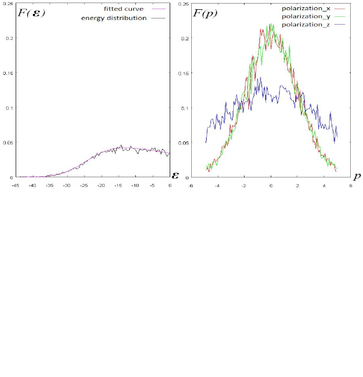
Figure 5: The energy distribution and its fitted curve (left picture) in ensemble of 1$D$ SSCs with the length of $L_{x}=25d_{0}$, which consists of $10^{4}$ spin-chains. Evidently there is only one global maximum for energy distribution. In the right picture polarization distributions are shown correspondingly on coordinates $x,y$ and $z$.

Thus as calculations show Birkhoff ergodic hypothesis Birkhoff may be used for ensembles which consist of $M\sim N_{x}^{2}$ spin-chains in order to change the summation of spin-chains on the integration by the energy distribution of the ensemble. The energy distribution of ensemble does not depend on the length of the spin-chain in the limit of ergodicity and it can be fitted very precisely with Eckart function Eckart (see FIG 5, the smooth

$$F(\varepsilon)=C(a,b,c,\gamma)\biggl{\{}\frac{a}{b+e^{-2\gamma\varepsilon}}+\frac{c\gamma^{2}}{(e^{-\gamma\varepsilon}+e^{\gamma\varepsilon})^{2}}\biggr{\}},$$ (22)

where $a,b,c$ and $\gamma$ some constants, in addition $C$ is a normalization constant and can be found from the condition:

$$\int_{-\infty}^{0}F(\varepsilon)d\varepsilon=1.$$ (23)

By placing (22) into (23) we can find:

$$C^{-1}(a,b,c,\gamma)=\frac{a}{2b\gamma}\ln(1+b)+\frac{c\gamma}{4}.$$ (24)

After fitting the energy distribution by means of analytical function (22) we find values of constants by entering into the function: $a=131.4,\,b=3138.2,\,\,c=-1.20344$ and $\gamma=0.162174.$

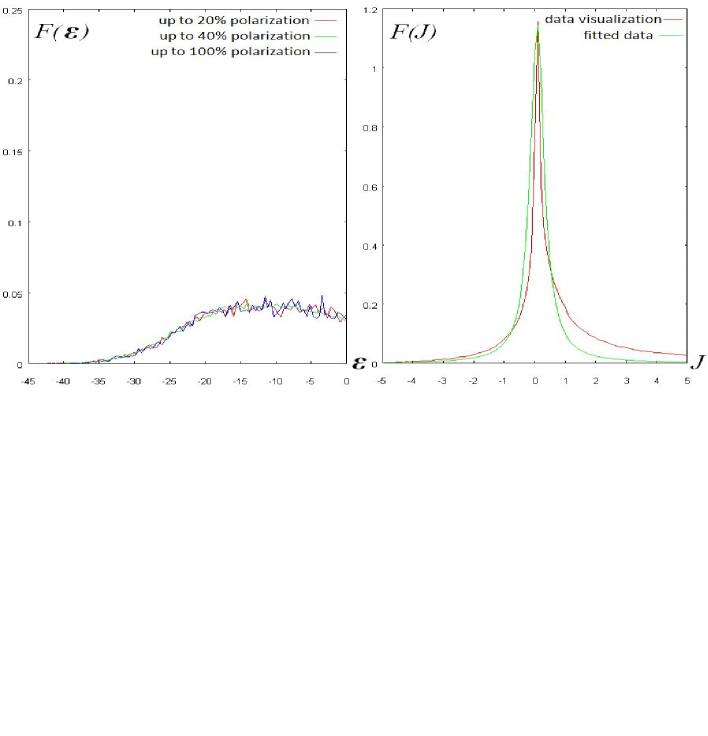
Figure 6: The energy distributions for ensembles consisting of 1$D$ SSCs of the length $L_{x}=25d_{0}$, with spin-chains polarization correspondingly up to $20,\,40$ and $100$ percents (left picture). Note that all the ensembles consist of $10^{4}$ spin-chains and their distributions practically do not differ. On the right picture the distribution of the spin-spin interaction constant is shown which differs essentially from Gauss-Edwards-Anderson distribution model (2).

We have also calculated 1$D$ SSCs ensemble with the length of spin-chains 25$d_{0}$ and correspondingly with polarizations of spin-chains up to 20,  40,  and 100 percents (see Fig 6, the left picture). In particular, as it follows from the picture the energy distribution does not depend on the degree of spin-chains polarization. We also have conducted simulation of ensembles which consist of spin-chains with lengths $100d_{0}$ and $1000d_{0}$ correspondingly. As the numerical modeling shows, statistical properties of ensembles are similar. In the considered cases distributions of energy concentrate correspondingly on scales $100d_{0}$ and $1000d_{0}$. Limits of ergodicities of ensembles are also investigated and it is shown that in these cases too it is of an order $N_{x}^{2}$.

Finally it is important to note that the distribution of spin-spin interaction constant is not defined apriori with the help of expression (2) but with the mass calculations of equations (6). On the basis of the obtained numerical data, the distribution of interaction constant $W(J)\equiv F(J)$ is constructed (see Fig 6, the right picture) from which it follows, that it essentially differs from the Gauss-Edwards-Anderson distribution model (2). The obtained distribution relatively is well fitted by the normalized to the unit of nonsymmetric Cauchy function Spiegle :

$$F(J)=\frac{g+\beta J}{\pi\bigl{[}g^{2}+(J-a_{0})^{2}\bigr{]}}.$$ (25)

where $g,\,\beta$ and $a_{0}$ are some adjusting parameters which are found from the condition of a good approximation of the data visualization curve. In the considered case they are correspondingly equal to: $g=0.27862,\,\beta=0.009$ and $a_{0}=0.083236$. Nevertheless, as the detailed analysis of curve of numerical data visualization shows (in particular its asymptotes) the distribution of interaction constant can be approximated precisely by Lev́y skew alpha-stable distribution function. Let us recall that Lev́y skew alpha-stable distribution is a continuous probability and a limit of certain random process $X(\alpha,\beta,\gamma,\delta;k)$ where parameters describe correspondingly: an index of stability or characteristic exponent $\alpha\in(0;2]$, a skewness parameter $\beta\in[-1;1]$, a scale parameter $\gamma>0$, a location parameter $\delta\in\mathbb{R}$ and an integer $k$ shows the certain parametrization (see in more detailed references Ibragimov ; Nolan ). Let us note, that the mean of distribution and its variance are infinite. However, taking into account that spin-spin interaction constant has limited value in real physical systems, it is possible to calculate distribution mean and its variance. In particular if $J\in[-5,+5]$ then $\overline{J}=0.50113$ and $\overline{J^{2}}=2,1052$.

IV Conclusion

The investigation of statistical properties of classical spin-glass system of various sizes is very important for understanding possibilities of effective influence and control over parameters of medium with the help of weak external fields. Evidently, when we put the spin-glass in external field the space-time periods define scales on which probably an essential changes in medium occur. For simplicity we suppose that the spin-glass system is an ensemble which consists of disordered 1$D$ steric spin-chains of $L_{x}$ lengths, between which interaction is absent (ideal ensemble). This type of classical ensemble is described by Heisenberg Hamiltonian (2). We have researched conditions of arising of stable spin-chains Eqs. (11) and nonequalities (9) and found a latent connection between random variables (see expression (19)), which shows that the distribution for spin-spin interaction constant can not be described by Guss-Edwards-Anderson model. In the result of equations of stationary points analysis (11) we have found system of recurrent equations (20) and new conditions (21). On the basis of obtained mathematical formulas the effective parallel algorithm for numerical simulation is developed which was realized on the example of the ensemble which consists of 1$D$ SSCs with length 25$d_{0}$. Similar to the dynamical systems, we have introduced the idea of Birkhoff ergodic hypothesis Birkhoff for the statical spin-glass systems. In this case the number of spin-chains of ensemble plays a role of the natural or ”timing” parameter of the system. Numerical simulations show that the ergodic hypothesis may be used for the case when ensemble consists of $M\propto N_{x}^{2}$ spin-chains in order to change the summation of spin-chains on the integration by the energy (polarization, etc.) distribution of the ensemble.

In particular, we have made numerical experiments for ensembles which include $10^{2}$,   $2\cdot 10^{3}$ and $10^{4}$ spin-chains. As it was shown by simulations in the case when $M\ll N_{x}^{2}$ for an ensemble, they are characteristic dimensional effects in energy distribution (the left picture on FIG 3). When the number of spin-chains is $M$ of order $2\cdot 10^{3}$ or more $10^{4}$, dimensional effects disappear and correspondingly energy distribution functions have one global maximum (see left pictures on FIG 4 and FIG 5). As it was shown, when increasing spin-chains number, the total and partial polarizations of the ensemble disappear. Let us note, that at modelling by algorithm (see scheme on FIG 2) condition (19) specifies the region of localization of random interaction constant $J_{i\,i+1}$ which depends on angular configurations $(i-1)$-th and $i$-th spins and interaction constant $J_{i-1\,i}$ between them. As a result, it allows to accelerate calculations of each spin-chain and hence the speed of parallel calculations of ensemble is increased essentially.

Finally it is important to note that it is proved, that the spin-spin interaction constant $J_{i\,i+1}$ has a form of Lev́y skew alpha-stable distribution (see the right picture on FIG 6). The considered scheme of solution of 1$D$ steric spin-glass problem can be used in different applied fields (see e.g. Helmut ). It can also be useful for analyzing 3$D$ spin-glass problem and creation of an effective parallel simulation algorithm of the spin-glass system with large dimensionality.

References

- (1) K. Binder and A. P. Young, Spin glasses: Experimental facts, theoretical concepts, and open questions. Rev. Mod. Physics, 58(4), 801-976 (1986).
- (2) M. Mézard, G. Parisi, M. A. Virasoro, Spin Glass Theory and Beyond (World Scientific, Singapore, 1987)
- (3) A. P. Young (ed.), Spin Glasses and Random Fields (World Scientific, Singapore, 1998)
- (4) R. Fisch and A. B. Harris, Spin-glass model in continuous dimensionality, Phys. Rev. Let., 47, 620 (1981).
- (5) A. Bovier, Statistical Mechanics of Disordered Systems: A Mathematical Perspective, Cambridge Series in Statistical and Probabilistic Mathematics, p 308 (2006).
- (6) Y. Tu, J. Tersoff and G. Grinstein, Structure and Energetic of the and Interface, Phys. Rev. Lett., 81, 4899 (1998).
- (7) K. V. R. Chary, G. Govil, NMR in Biological Systems: From Molecules to Human (Focus on Structural Biology 6), Springer, p 511, (2008).
- (8) E. Baake, M. Baake and H. Wagner, Ising Quantum Chain is a Equivalent to a Model of Biological Evolution, Phys. Rev. Let., 78(3), 559-562 (1997.)
- (9) A S Gevorkyan et al., New Mathematical Conception and Computation Algorithm for Study of Quantum 3D Disordered Spin System Under the Influence of External Field, Trans. On Comput. Sci., VII, LNCS 132-153, Spinger-Verlage, 10.1007/978-3-642-11389-58
- (10) S. F. Edwards and P. W. Anderson, Theory of spin glasses, J. Phys. F 9, 965 (1975).
-
(11)
J. von Neuman, Physical Applications of the
Ergodic Hypothesis, Proc. Nat. Acad. Sci. USA, 18(3):
263-266 (1932).
G. D. Birkhoff, What is ergodic theorem? American Mathematical Monthly, 49(4): 222-226 (1931). - (12) S. Flügge, Practical Quantum Mechanics I, (Springer-Verlag, Berlin-Heidelberg- New York 1971).
- (13) M. R. Spiegle, Theory and Problems of Probability and Stochastics, (New-York, McGraw-Hill, pp 114-115, 1992).
- (14) I. Ibragimov and Yu. Linnik, Independent and Stationary Sequences of Random Variebles, (Wolters-Noordhoff Publishing Groningen, The Netherlands 1971).
- (15) J. P. Nolan, Stable Distributions: Models for Heavy Tailed Data (2009-02-21). .
- (16) H. G. Katzgraber, A. K. Hartmann and A. P. Young, New Insights from One-Dimensional Spin Glasses, (2008) ArXiv:0803.3417v1 [cond-mat.dis-nn].