Manipulating quantum information on the controllable systems or subspaces

Abstract

In this paper, we explore how to constructively manipulate qubits by rotating Bloch spheres. It is revealed that three-rotation and one-rotation Hamiltonian controls can be constructed to steer qubits when two tunable Hamiltonian controls are available. It is demonstrated in this research that local-wave function controls such as Bang-Bang, triangle-function and quadratic function controls can be utilized to manipulate quantum states on the Bloch sphere. A new kind of time-energy performance index is proposed to trade-off time and energy resource cost, in which control magnitudes are optimized in terms of this kind of performance. It is further exemplified that this idea can be generalized to manipulate encoded qubits on the controllable subspace.

I Introduction

Dating from the birth of quantum theory, control of quantum systems is an important issue [1]. Quantum control theory has been developed ever since 1980s[2, 3, 4]. Recently, quantum information and quantum computation is the focus of reseach[5]. A great progress has been made in the domain of quantum control[6, 7], in which the controllability of quantum systems is a fundamental issue. The different notations of controllability have been explored in [8, 9, 10, 11, 12, 13, 14]. Specially, the controllability of quantum open systems has been studied by some researchers[15, 16, 17, 18]. It is quite well known that quantum open systems are not open-loop controllable but there may exist decoherence-free subsystems or subspaces[19, 20, 21, 22, 23]. The works on encoded universality[24, 25] further enhance the belief that one can manipulate quantum information on the encoded subspace. Optimal control theory has also been successfully applied to the design of open-loop coherent control strategies in physical chemistry[26, 27, 28]. Recently, time-optimal control problems for spin systems have been solved to achieve specified control objectives in minimum time[29, 30, 31]. On the other hand, the challenge of open-loop control is to design external fields or potentials acting as model-relied controls. The main strategies for open-loop control design seem to be based either on geometric ideas or more formally Lie group decompositions, as in[32, 33, 34, 35, 36].

In this paper, we explore how to constructively manipulate qubits or encoded qubits based on the geometric parametrization of qubits when two tunable Hamiltonian controls are available. It is demonstrated that one can not only design $3$-rotation Hamiltonian controls to manipulate qubits, but can also construct $1$-rotation Hamiltonian controls to steer qubits by carefully choosing a rotation axis. It should be underlined that local wave controls can be constructed to manipulate qubits corresponding to each rotation. Furthermore, we proposed a new kind of time-energy performance index

$$J=\lambda\cdot{t_{f}}+\int_{0}^{t_{f}}E(u(t))dt=\int_{0}^{t_{f}}[\lambda+E(u(t))]dt$$ (1)

where $E(u(t))$ is the energy cost of control at time $t$, $t_{f}$ is free terminal time, and $\lambda$ is introduced as a ratio parameter to trade-off the cost of time and energy resource. It has also been discussed in [36] how to optimize $3$-rotation Bang-Bang controls to transfer quantum state in terms of this kind of time-energy performance. In this paper, we comprehensively discuss how to optimize control magnitudes in terms of this kind of time-energy performance for both $3$-rotation and $1$-rotation controls, and present optimal Bang-Bang, triangle-function and quadratic function controls, respectively.

The rest of this paper are organized as follows. In Sect. II, we present prerequisite for further discussion. It is illustrated in Sect. III how to manipulate qubit by $3$-rotation Bang-Bang, triangle-function, and quadratic function controls. The optimal controls are further presented in the sense of time-energy performance. It is also revealed in Sect. IV that one can utilize three kinds of local-wave controls to manipulate qubits just by one-times rotation. The paper concludes with Sect. V.

II Prerequisite

Consider a controlled qubit governed by the equation

$$\frac{d}{dt}|\psi(t)\rangle=-\frac{{i}}{\hbar}H(t)|\psi(t)\rangle=-\frac{{i}}{\hbar}[u_{z}(t)\sigma_{z}+u_{y}(t)\sigma_{y}]|\psi(t)\rangle$$ (2)

where $\sigma_{z}=I_{2}-2|1\rangle\langle 1|$ and $\sigma_{y}=i|1\rangle\langle 0|-i|0\rangle\langle 1|$. For simplicity, we set $\hbar=1$.

Denote $|u_{+}\rangle=\cos\frac{\theta_{u}}{2}|0\rangle+i\sin\frac{\theta_{u}}{2}|1\rangle;|u_{-}\rangle=\sin\frac{\theta_{u}}{2}|0\rangle-i\cos\frac{\theta_{u}}{2}|1\rangle$. It is interesting to point out that if $H(t)=f(t)[\cos\theta_{u}\sigma_{z}+\sin\theta_{u}\sigma_{y}]$, then one can express the Hamiltonian $H(t)$ as $H(t)=f(t)\sigma^{u}_{z}$ where $\sigma^{u}_{z}=|u_{+}\rangle\langle{u_{+}}|-|u_{-}\rangle\langle{u_{-}}|$.

(a) $3$-rotation trajectories

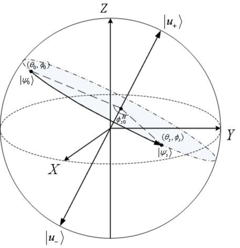
(b) $1$-rotation trajectory

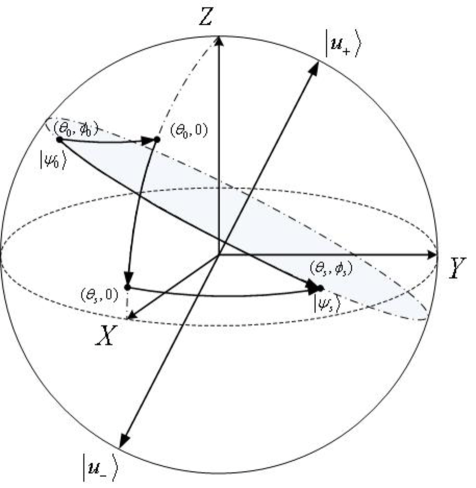
(c) $3$- and $1$-rotation trajectories

Figure 1: trajectories on the Bloch sphere

As shown in Fig.1, one can not only choose $3$-rotation control functions to steer the controlled qubit system from an arbitrary initial state to another arbitrary target state, but can also construct $1$-rotation control function $f(t)$ to achieve the same goal.

In this paper, we will just concentrate on three kind of local wave-functions: a piece-wise constant function (Bang-Bang control), a triangle-function and a quadratic function.

Denote the triangle function $u_{T}(t;t_{0},t_{1},L)$ and the quadratic function $u_{Q}(t;t_{0},t_{1},L)$ respectively as follows:

$$u_{T}(t;t_{0},t_{1},L)=\bigg{\{}\begin{array}[]{cc}\frac{2L}{t_{1}-t_{0}}\cdot{(t-t_{0})}&t\in[t_{0},\frac{t_{0}+t_{1}}{2})\\ -\frac{2L}{t_{1}-t_{0}}\cdot{(t-t_{1})}&t\in[\frac{t_{0}+t_{1}}{2},t_{1})\\ 0&otherwise\end{array}$$ (3)

and

$$u_{Q}(t;t_{0},t_{1},L)=\bigg{\{}\begin{array}[]{cc}\frac{4L\cdot{(t-t_{0})(t_{1}-t)}}{(t_{1}-t_{0})^{2}}&t\in[t_{0},t_{1}]\\ 0&otherwise\end{array}$$ (4)

where both $u_{T}(t;t_{0},t_{1},L)$ and $u_{Q}(t;t_{0},t_{1},L)$ are nonzero only when $t\in(t_{0},t_{1})$, and take the maximum magnitude $L$ at time $\frac{t_{0}+t_{1}}{2}$. It should be underlined that the pulse area of the control pulses is the key control variable for geometric control and the pulse area inequality for Bang-Bang, triangle-function and quadratic function controls is given as

$$\int^{t_{1}}_{t_{0}}u_{T}(t;t_{0},t_{1},L)dt<\int^{t_{1}}_{t_{0}}u_{Q}(t;t_{0},t_{1},L)dt<\int^{t_{1}}_{t_{0}}Ldt=L(t_{1}-t_{0})$$ (5)

Furthermore, it is worth pointing out that $\int^{t_{1}}_{t_{0}}L^{2}dt=L^{2}(t_{1}-t_{0})$ and

$$E(u_{T}(t;t_{0},t_{1},L))=\int^{t_{1}}_{t_{0}}|u_{T}(t;t_{0},t_{1},L)|^{2}dt=\frac{1}{3}L^{2}(t_{1}-t_{0})$$ (6)

and

$$E(u_{Q}(t;t_{0},t_{1},L))=\int^{t_{1}}_{t_{0}}|u_{Q}(t;t_{0},t_{1},L)|^{2}dt=\frac{8}{15}L^{2}(t_{1}-t_{0})$$ (7)

Remark: We would like to further emphasize that that one can construct both $3$-rotation and $1$-rotation local wave-function controls to manipulate qubits if $H(t)=u_{x}(t)\sigma_{x}+u_{y}(t)\sigma_{y}$ or $H(t)=u_{z}(t)\sigma_{z}+u_{x}(t)\sigma_{x}$. In other words, $3$-rotation and $1$-rotation controls can be constructed as long as two tunable Hamiltonian controls are available.

III Manipulate qubit by three rotations

Consider a controlled qubit governed by the equation

$$\frac{d}{dt}|\psi(t)\rangle=-{i}(u_{z}(t)\sigma_{z}+u_{y}(t)\sigma_{y})|\psi(t)\rangle$$ (8)

with an initial state $|\psi_{0}\rangle=\cos\frac{\theta_{0}}{2}|0\rangle+e^{i\phi_{0}}\sin\frac{\theta_{0}}{2}|1\rangle$ and a target state $|\psi_{s}\rangle=\cos\frac{\theta_{s}}{2}|0\rangle+e^{i\phi_{s}}\sin\frac{\theta_{s}}{2}|1\rangle$. For the sake of the following analysis in this section, we denote $\phi_{0m}=\min(\phi_{0},2\pi-\phi_{0})$, $\phi_{sm}=\min(\phi_{s},2\pi-\phi_{s})$, $\theta_{0s}=|\theta_{s}-\theta_{0}|$ and $\Sigma_{\phi\theta}=\phi_{0m}+\theta_{0s}+\phi_{sm}$.

In this section, our control goal is to find $t_{f}$ and some form of controls $\{u_{z}(t),u_{y}(t):0\leq{t}\leq{t_{f}}\}$ so that

$$|\psi(t_{f})\rangle=|\psi_{s}\rangle$$ (9)

by three rotations about $z-$axis, $y-$axis and $z-$axis, respectively. Furthermore, we hope to optimize control magnitude in terms of the performance (1) where $E(u(t))=|u_{z}(t)|^{2}+|u_{y}(t)|^{2}$ and $\lambda>0$.

III-A $3$-rotation Bang-Bang controls

In this subsection, we will discuss how to manipulate quantum system (8) by three-rotation Bang-Bang control. According to the properties of Pauli matrices[5], we choose the piecewise constant controls $\{u_{z}(t),u_{y}(t):0\leq{t}\leq{t_{f}}\}$ as follows:

$$u_{z}(t)=\bigg{\{}\begin{array}[]{cc}sign(\phi_{0}-\pi)M_{z1}&t\in[0,t_{1})\\ 0&t\in[t_{1},t_{2})\\ sign(\pi-\phi_{s})M_{z2}&t\in[t_{2},t_{f}]\end{array}$$ (10)

and

$$u_{y}(t)=\bigg{\{}\begin{array}[]{cc}0&t\in[0,t_{1})\\ sign(\theta_{s}-\theta_{0})M_{y}&t\in[t_{1},t_{2})\\ 0&t\in[t_{2},t_{f}]\end{array}$$ (11)

where $t_{1}=\frac{\phi_{0m}}{2M_{z1}}$, $t_{2}=\frac{\theta_{0s}}{2M_{y}}+t_{1}$ and $t_{f}=\frac{\phi_{sm}}{2M_{z2}}+t_{2}$.

After some calculations, we have $|\psi(t_{1})\rangle=\cos\frac{\theta_{0}}{2}|0\rangle+\sin\frac{\theta_{0}}{2}|1\rangle$, $|\psi(t_{2})\rangle=\cos\frac{\theta_{s}}{2}|0\rangle+\sin\frac{\theta_{s}}{2}|1\rangle$, and $|\psi(t_{f})\rangle=\cos\frac{\theta_{s}}{2}|0\rangle+e^{i\phi_{s}}\sin\frac{\theta_{s}}{2}|1\rangle$.

Next, our task is to choose $M_{z1}$, $M_{z2}$ and $M_{y}$ to minimize the performance (1). It can be demonstrated that

$$\begin{array}[]{c}J=\lambda(\frac{\phi_{0m}}{2M_{z1}}+\frac{\theta_{0s}}{2M_{y}}+\frac{\phi_{sm}}{2M_{z2}})+(\frac{M_{z1}\phi_{0m}}{2}+\frac{M_{y}\theta_{0s}}{2}+\frac{M_{z2}\phi_{sm}}{2})\geq\sqrt{\lambda}\Sigma_{\phi\theta}\end{array}$$ (12)

where the equality holds only if $M_{z1}=M_{z2}=M_{y}=\sqrt{\lambda}$.

If only bounded Bang-Bang controls with bound $L_{B}$ are permitted, then the optimal controls are given as:

$$u^{*}_{z}(t)=\bigg{\{}\begin{array}[]{cc}sign(\phi_{0}-\pi)L_{B}^{*}&t\in[0,t^{*}_{1})\\ 0&t\in[t^{*}_{1},t^{*}_{2})\\ sign(\pi-\phi_{s})L_{B}^{*}&t\in[t^{*}_{2},t^{*}_{f}]\end{array}$$ (13)

and

$$u^{*}_{y}(t)=\bigg{\{}\begin{array}[]{cc}0&t\in[0,t^{*}_{1})\\ sign(\theta_{s}-\theta_{0})L_{B}^{*}&t\in[t^{*}_{1},t^{*}_{2})\\ 0&t\in[t^{*}_{2},t^{*}_{f}]\end{array}$$ (14)

where $t^{*}_{1}=\frac{\phi_{0m}}{2L_{B}^{*}}$, $t^{*}_{2}=\frac{\theta_{0s}}{2L_{B}^{*}}+t^{*}_{1}$, $t^{*}_{fB}=\frac{\phi_{sm}}{2L_{B}^{*}}+t^{*}_{2}=\frac{\Sigma_{\phi\theta}}{2L_{B}^{*}}$ and $L_{B}^{*}=\min(\sqrt{\lambda},L_{B})$. Furthermore, the corresponding optimal performance is $J_{B}^{*}=(\frac{\lambda}{2L_{B}^{*}}+\frac{L_{B}^{*}}{2})\Sigma_{\phi\theta}$. It is interesting to underline that $J_{B}^{*}=\lambda\cdot{t^{*}_{fB}}+E^{*}_{B}$ where $E^{*}_{B}=\frac{1}{2}L_{B}^{*}\Sigma_{\phi\theta}$, and ${t^{*}_{fB}}\cdot{E^{*}_{B}}=\frac{1}{4}\Sigma_{\phi\theta}^{2}$ only depends on the location of both initial and target states on the Bloch sphere.

If unbounded Bang-Bang controls are permitted, we have $L_{B}^{*}=\sqrt{\lambda}$, $t^{*}_{fB}=\frac{\Sigma_{\phi\theta}}{2\sqrt{\lambda}}$, $E^{*}_{B}=\frac{\sqrt{\lambda}}{2}\Sigma_{\phi\theta}$ and $J_{B}^{*}=\sqrt{\lambda}\Sigma_{\phi\theta}$, therefore ${t^{*}_{fB}}\cdot{E^{*}_{B}}=\frac{1}{4}\Sigma_{\phi\theta}^{2}$.

III-B $3$-rotation triangle-function controls

In this subsection, we will first demonstrate that the target state $|\psi(t_{f})\rangle=|\psi_{s}\rangle$ can be achieved from the initial state $|\psi_{o}\rangle$ by the following three-rotation triangle-function controls:

$$u_{z}(t)=sign(\phi_{0}-\pi)u_{T}(t;0,t_{1},M_{z1})+sign(\pi-\phi_{s})u_{T}(t;t_{2},t_{f},M_{z2})$$ (15)

and

$$u_{y}(t)=sign(\theta_{s}-\theta_{0})u_{T}(t;t_{1},t_{2},M_{y})$$ (16)

where $t_{1}=\frac{\phi_{0m}}{M_{z1}}$, $t_{2}=\frac{\theta_{0s}}{M_{y}}+t_{1}$ and $t_{f}=\frac{\phi_{sm}}{M_{z2}}+t_{2}$. It can be proved that $|\psi(t_{1})\rangle=\cos\frac{\theta_{0}}{2}|0\rangle+\sin\frac{\theta_{0}}{2}|1\rangle$, $|\psi(t_{2})\rangle=\cos\frac{\theta_{s}}{2}|0\rangle+\sin\frac{\theta_{s}}{2}|1\rangle$, and $|\psi(t_{f})\rangle=\cos\frac{\theta_{s}}{2}|0\rangle+e^{i\phi_{s}}\sin\frac{\theta_{s}}{2}|1\rangle$.

Subsequently, our task is to select magnitude $M_{z1}$, $M_{z2}$ and $M_{y}$ to minimize the performance (1). It can be demonstrated that

$$\begin{array}[]{c}J=\lambda(\frac{\phi_{0m}}{M_{z1}}+\frac{\theta_{0s}}{M_{y}}+\frac{\phi_{sm}}{M_{z2}})+(\frac{M_{z1}\phi_{0m}}{3}+\frac{M_{y}\theta_{0s}}{3}+\frac{M_{z2}\phi_{sm}}{3})\geq\frac{2\sqrt{\lambda}}{\sqrt{3}}\Sigma_{\phi\theta}\end{array}$$ (17)

where the equality holds only if $M_{z1}=M_{z2}=M_{y}=\sqrt{3\lambda}$. If only bounded triangle-function controls with bound $L_{B}$ are permitted, then the optimal $3$-rotation triangle-function controls are given as:

$$u^{*}_{z}(t)=sign(\phi_{0}-\pi)u_{T}(t;0,t^{*}_{1},L_{T}^{*})+sign(\pi-\phi_{s})u_{T}(t;t^{*}_{2},t^{*}_{fT},L_{T}^{*})$$ (18)

and

$$u^{*}_{y}(t)=sign(\theta_{s}-\theta_{0})u_{T}(t;t^{*}_{1},t^{*}_{2},L_{T}^{*})$$ (19)

where $t^{*}_{1}=\frac{\phi_{0m}}{L_{T}^{*}}$, $t^{*}_{2}=\frac{\theta_{0s}}{L_{T}^{*}}+t^{*}_{1}$, $t^{*}_{fT}=\frac{\Sigma_{\phi\theta}}{L_{T}^{*}}$ and $L_{T}^{*}=\min(\sqrt{3\lambda},L_{B})$. Furthermore, the optimal performance corresponding to bounded triangle-function control is $J_{T}^{*}=(\frac{\lambda}{L_{T}^{*}}+\frac{L_{T}^{*}}{3})\Sigma_{\phi\theta}$. It is interesting to underline that $J_{T}^{*}=\lambda\cdot{t^{*}_{fT}}+E^{*}_{T}$ with $E^{*}_{T}=\frac{1}{3}L_{T}^{*}\Sigma_{\phi\theta}$, and ${t^{*}_{fT}}\cdot{E^{*}_{T}}=\frac{1}{3}\Sigma_{\phi\theta}^{2}$ only depends on the location of both initial and target states on the Bloch sphere.

If unbounded triangle-function controls are permitted, then we have $t^{*}_{fT}=\frac{\Sigma_{\phi\theta}}{\sqrt{3\lambda}}$, $L_{T}^{*}=\sqrt{3\lambda}$, $E^{*}_{T}=\frac{\sqrt{3\lambda}}{3}\Sigma_{\phi\theta}$ and $J_{T}^{*}=\frac{2\sqrt{\lambda}}{\sqrt{3}}\Sigma_{\phi\theta}$, thus ${t^{*}_{fT}}\cdot{E^{*}_{T}}=\frac{1}{3}\Sigma_{\phi\theta}^{2}$.

III-C $3$-rotation quadratic function controls

In this subsection, it is demonstrated that the target state $|\psi(t_{f})\rangle=|\psi_{s}\rangle$ can be achieved from the initial state $|\psi_{o}\rangle$ by the following quadratic controls:

$$u_{z}(t)=sign(\phi_{0}-\pi)u_{Q}(t;0,t_{1},M_{z1})+sign(\pi-\phi_{s})u_{Q}(t;t_{2},t_{f},M_{z2})$$ (20)

and

$$u_{y}(t)=sign(\theta_{s}-\theta_{0})u_{Q}(t;t_{1},t_{2},M_{y})$$ (21)

where $t_{1}=\frac{3\phi_{0m}}{4M_{z1}}$, $t_{2}=\frac{3\theta_{0s}}{4M_{y}}+t_{1}$ and $t_{f}=\frac{3\phi_{sm}}{4M_{z2}}+t_{2}$. It can be confirmed that $|\psi(t_{1})\rangle=\cos\frac{\theta_{0}}{2}|0\rangle+\sin\frac{\theta_{0}}{2}|1\rangle$, $|\psi(t_{2})\rangle=\cos\frac{\theta_{s}}{2}|0\rangle+\sin\frac{\theta_{s}}{2}|1\rangle$, and $|\psi(t_{f})\rangle=\cos\frac{\theta_{s}}{2}|0\rangle+e^{i\phi_{s}}\sin\frac{\theta_{s}}{2}|1\rangle$.

Next, our task is to choose magnitude $M_{z1}$, $M_{z2}$ and $M_{y}$ to minimize the performance (1).

After some calculations, we have

$$\begin{array}[]{c}J=\lambda(\frac{3\phi_{0m}}{4M_{z1}}+\frac{3\theta_{0s}}{4M_{y}}+\frac{3\phi_{sm}}{4M_{z2}})+(\frac{2M_{z1}\phi_{0m}}{5}+\frac{2M_{y}\theta_{0s}}{5}+\frac{2M_{z2}\phi_{sm}}{5})\geq\frac{{\sqrt{30\lambda}}}{5}\Sigma_{\phi\theta}\end{array}$$ (22)

where the equality holds only if $M_{z1}=M_{z2}=M_{y}=\frac{\sqrt{30\lambda}}{4}$.

If only bounded quadratic function controls with bound $L_{B}$ are permitted, the optimal $3$-rotation bounded quadratic-function controls are given as:

$$u^{*}_{z}(t)=sign(\phi_{0}-\pi)u_{Q}(t;0,t^{*}_{1},L_{Q}^{*})+sign(\pi-\phi_{s})u_{Q}(t;t^{*}_{2},t^{*}_{f},L_{Q}^{*})$$ (23)

and

$$u^{*}_{y}(t)=sign(\theta_{s}-\theta_{0})u_{Q}(t;t^{*}_{1},t^{*}_{2},L_{Q}^{*})$$ (24)

where $t^{*}_{1}=\frac{3\phi_{0m}}{4L_{Q}^{*}}$, $t^{*}_{2}=\frac{3\theta_{0s}}{4L_{Q}^{*}}+t_{1}$, $t^{*}_{fQ}=\frac{3\Sigma_{\phi\theta}}{4L_{Q}^{*}}$ and $L_{Q}^{*}=\min(\frac{\sqrt{30\lambda}}{4},L_{B})$. Moreover, the optimal performance corresponding to bounded control is $J_{Q}^{*}=(\frac{3\lambda}{4L_{Q}^{*}}+\frac{2L_{Q}^{*}}{5})\Sigma_{\phi\theta}$. It is interesting to underline that $J_{Q}^{*}=\lambda\cdot{t^{*}_{fQ}}+E^{*}_{Q}$ where $E^{*}_{Q}=\frac{2}{5}L_{Q}^{*}\Sigma_{\phi\theta}$, and ${t^{*}_{fQ}}\cdot{E^{*}_{Q}}=\frac{3}{10}\Sigma_{\phi\theta}^{2}$ only depends on the location of both initial and target states on the Bloch sphere.

If unbounded quadratic function controls are permitted, we have $t^{*}_{fQ}=\frac{3\Sigma_{\phi\theta}}{\sqrt{30\lambda}}$, $L_{Q}^{*}=\frac{\sqrt{30\lambda}}{4}$, $E^{*}_{Q}=\frac{\sqrt{30\lambda}}{10}\Sigma_{\phi\theta}$ and $J_{Q}^{*}=\frac{\sqrt{30\lambda}}{5}\Sigma_{\phi\theta}$, therefore ${t^{*}_{fQ}}\cdot{E^{*}_{Q}}=\frac{3}{10}\Sigma_{\phi\theta}^{2}$.

Remark: 1. When unbounded controls are permitted, it has been demonstrated in this section that $J^{*}_{B}<J^{*}_{Q}<J^{*}_{T}$, $E^{*}_{B}<E^{*}_{Q}<E^{*}_{T}$ and $t^{*}_{fB}<t^{*}_{fQ}<t^{*}_{fT}$, therefore we have $t^{*}_{fB}{\cdot}E^{*}_{B}<t^{*}_{fQ}{\cdot}E^{*}_{Q}<t^{*}_{fT}{\cdot}E^{*}_{T}$.

2. Even when only bounded controls are permitted, the above inequalities are valid for all $\lambda$ and $L_{B}$ except that $E^{*}_{B}<E^{*}_{Q}<E^{*}_{T}$ does not hold for some $\lambda$ and $L_{B}$.

IV Manipulate qubits just by one rotation

Reconsider the controlled qubit (8) with both the same initial and target states given in the Section III. In this section, our control goal is to find $t_{f}$ and some form of controls $\{u_{z}(t),u_{y}(t):0\leq{t}\leq{t_{f}}\}$ so that $|\psi(t_{f})\rangle=|\psi_{s}\rangle$ is attained just by one rotation. Furthermore, we hope to choose $\{u_{z}(t),u_{y}(t):0\leq{t}\leq{t_{f}}\}$ to minimize the performance (1).

Choose $H(t)=f(t)(\cos\theta_{u}\sigma_{z}+\sin\theta_{u}\sigma_{y})$ with $\theta_{u}\in[0,\pi]$ so that the following equation holds

$$\sin\theta_{u}\sin\theta_{0}\sin\phi_{0}+\cos\theta_{u}\cos\theta_{0}=\sin\theta_{u}\sin\theta_{s}\sin\phi_{s}+\cos\theta_{u}\cos\theta_{s}$$ (25)

Since $|0\rangle=\cos\frac{\theta_{u}}{2}|u_{+}\rangle+i\sin\frac{\theta_{u}}{2}|u_{-}\rangle;|1\rangle=-i\sin\frac{\theta_{u}}{2}|u_{+}\rangle+i\cos\frac{\theta_{u}}{2}|u_{-}\rangle$, the initial and target states can be expressed in terms of the new basis $|u_{+}\rangle$ and $|u_{-}\rangle$ as follows

$$|\psi_{0}\rangle=\cos\frac{\theta^{H}_{s0}}{2}|u_{+}\rangle+e^{i\phi^{H}_{0}}\sin\frac{\theta^{H}_{s0}}{2}|u_{-}\rangle$$ (26)

and

$$|\psi_{s}\rangle=\cos\frac{\theta^{H}_{s0}}{2}|u_{+}\rangle+e^{i\phi^{H}_{s}}\sin\frac{\theta^{H}_{s0}}{2}|u_{-}\rangle$$ (27)

where

$$\cos\frac{\theta^{H}_{s0}}{2}=\sqrt{\frac{1}{2}+\frac{1}{2}[\sin\theta_{u}\sin\theta_{0}\sin\phi_{0}+\cos\theta_{u}\cos\theta_{0}]}$$ (28)

and

$$\begin{array}[]{c}\phi^{H}_{0}=-\angle(\cos\frac{\theta_{0}}{2}\cos\frac{\theta_{u}}{2}-ie^{i\phi_{0}}\sin\frac{\theta_{0}}{2}\sin\frac{\theta_{u}}{2})\\ +\angle(i\cos\frac{\theta_{0}}{2}\sin\frac{\theta_{u}}{2}+ie^{i\phi_{0}}\sin\frac{\theta_{0}}{2}\cos\frac{\theta_{u}}{2})\pm{2n_{0}}\pi\end{array}$$ (29)

and

$$\begin{array}[]{c}\phi^{H}_{s}=-\angle(\cos\frac{\theta_{s}}{2}\cos\frac{\theta_{u}}{2}-ie^{i\phi_{s}}\sin\frac{\theta_{s}}{2}\sin\frac{\theta_{u}}{2})\\ +\angle(i\cos\frac{\theta_{s}}{2}\sin\frac{\theta_{u}}{2}+ie^{i\phi_{s}}\sin\frac{\theta_{s}}{2}\cos\frac{\theta_{u}}{2})\pm{2n_{s}}\pi\end{array}$$ (30)

It is easy to prove that one can choose the suitable integers $n_{0}$ and $n_{s}$ so that $\phi^{H}_{0},\phi^{H}_{s}\in[0,2\pi)$.

Remark: 1. We would like to point out that the initial and target states have the same angle $\theta^{H}_{s0}$ about the control Hamiltonian axis as shown in Fig.1.

2. For the sake of the analysis, we introduce $\phi^{H}_{s0}=\min(|\phi^{H}_{s}-\phi^{H}_{0}|,2\pi-|\phi^{H}_{s}-\phi^{H}_{0}|)$ with $\phi^{H}_{s0}\in[0,\pi)$. It should be underlined that $\phi^{H}_{s0}$ depends not only on the location of both initial and target states on the Bloch sphere, but also on the Hamiltonian $H(t)$, i.e., the $y-z$ plane.

IV-A $1$-rotation Bang-Bang controls

In this subsection, we will discuss how to manipulate the quantum system (8) by Bang-Bang control. According to the aforementioned analysis in the section, we can choose the piecewise constant controls $\{f(t):0\leq{t}\leq{t_{f}}\}$ as follows:

$$f(t)=\bigg{\{}\begin{array}[]{cc}M_{ub},t\in[0,t_{f})&if0\pm{2k\pi}<(\phi^{H}_{s}-\phi^{H}_{0})<\pi\pm{2k\pi}\\ -M_{ub},t\in[0,t_{f})&if\pi\pm{2k\pi}\leq(\phi^{H}_{s}-\phi^{H}_{0})<2\pi\pm{2k\pi}\end{array}$$ (31)

where $t_{f}=\frac{\phi^{H}_{s0}}{2M_{ub}}$.

Subsequently, our task is to choose $M_{ub}$ to minimize the performance (1) where $E(u(t))=|f(t)|^{2}$ and $\lambda>0$.

After some careful calculations, we have

$$\begin{array}[]{c}J=\lambda\frac{\phi^{H}_{s0}}{2M_{ub}}+\frac{M_{ub}\phi^{H}_{s0}}{2}\geq\sqrt{\lambda}\phi^{H}_{s0}\end{array}$$ (32)

where the equality holds only if $M_{ub}=\sqrt{\lambda}$.

If only bounded Bang-Bang controls with bound $L_{B}$ are permitted, then the optimal controls are given as:

$$u^{*}_{z}(t)=\bigg{\{}\begin{array}[]{cc}\cos\theta_{u}L_{B}^{*},t\in[0,t^{*}_{fB})&if0\pm{2k\pi}\leq(\phi^{H}_{s}-\phi^{H}_{0})<\pi\pm{2k\pi}\\ -\cos\theta_{u}L_{B}^{*},t\in[0,t^{*}_{fB})&if\pi\pm{2k\pi}\leq(\phi^{H}_{s}-\phi^{H}_{0})<2\pi\pm{2k\pi}\end{array}$$ (33)

and

$$u^{*}_{y}(t)=\bigg{\{}\begin{array}[]{cc}\sin\theta_{u}L_{B}^{*},t\in[0,t^{*}_{fB})&if0\pm{2k\pi}\leq(\phi^{H}_{s}-\phi^{H}_{0})<\pi\pm{2k\pi}\\ -\sin\theta_{u}L_{B}^{*},t\in[0,t^{*}_{fB})&if\pi\pm{2k\pi}\leq(\phi^{H}_{s}-\phi^{H}_{0})<2\pi\pm{2k\pi}\end{array}$$ (34)

where $t^{*}_{fB}=\frac{\phi^{H}_{s0}}{2L_{B}^{*}}$ and $L_{B}^{*}=\min(\sqrt{\lambda},\frac{L_{B}}{\max(\cos\frac{\theta_{u}}{2},\sin\frac{\theta_{u}}{2})})$. The optimal performance corresponding to bounded Bang-Bang controls is $J_{B}^{*}=(\frac{\lambda}{2L_{B}^{*}}+\frac{L_{B}^{*}}{2})\phi^{H}_{s0}$. It is interesting to emphasize that optimal performance can be expressed as $J_{B}^{*}=\lambda\cdot{t^{*}_{fB}}+E^{*}_{B}$ with $E_{B}^{*}=\frac{L_{B}^{*}}{2}\phi^{H}_{s0}$, and $E^{*}_{B}\cdot{t^{*}_{fB}}=\frac{1}{4}(\phi^{H}_{s0})^{2}$ where $\phi^{H}_{s0}$ is independent of $\lambda$.

If unbounded Bang-Bang controls are permitted, then $L_{B}^{*}=\sqrt{\lambda}$, $t^{*}_{fB}=\frac{\phi^{H}_{s0}}{2\sqrt{\lambda}}$, $E_{B}^{*}=\frac{\sqrt{\lambda}}{2}\phi^{H}_{s0}$, and $J_{B}^{*}=\sqrt{\lambda}\phi^{H}_{s0}$. Therefore, $E^{*}_{B}\cdot{t^{*}_{fB}}=\frac{1}{4}(\phi^{H}_{s0})^{2}$.

IV-B $1$-rotation triangle-function controls

In this subsection, we will explore how to construct one-rotation triangle-function controls $\{f(t):0\leq{t}\leq{t_{f}}\}$ to achieve the target state from the initial state. We can select

$$f(t)=\bigg{\{}\begin{array}[]{cc}u_{T}(t;0,t_{f},M_{ut})&if0\pm{2k\pi}\leq(\phi^{H}_{s}-\phi^{H}_{0})<\pi\pm{2k\pi}\\ -u_{T}(t;0,t_{f},M_{ut})&if\pi\pm{2k\pi}\leq(\phi^{H}_{s}-\phi^{H}_{0})<2\pi\pm{2k\pi}\end{array}$$ (35)

where $t_{f}=\frac{\phi^{H}_{s0}}{M_{ut}}$. In other words, $\{u_{z}(t),u_{y}(t)\}$ can be constructed as follows:

$$u_{z}(t)=\bigg{\{}\begin{array}[]{cc}u_{T}(t;0,\frac{\phi^{H}_{s0}}{M_{ut}},M_{ut})\cos\theta_{u}&if0\pm{2k\pi}\leq(\phi^{H}_{s}-\phi^{H}_{0})<\pi\pm{2k\pi}\\ -u_{T}(t;0,\frac{\phi^{H}_{s0}}{M_{ut}},M_{ut})\cos\theta_{u}&if\pi\pm{2k\pi}\leq(\phi^{H}_{s}-\phi^{H}_{0})<2\pi\pm{2k\pi}\end{array}$$ (36)

and

$$u_{y}(t)=\bigg{\{}\begin{array}[]{cc}u_{T}(t;0,\frac{\phi^{H}_{s0}}{M_{ut}},M_{ut})\cos\theta_{u}&if0\pm{2k\pi}\leq(\phi^{H}_{s}-\phi^{H}_{0})<\pi\pm{2k\pi}\\ -u_{T}(t;0,\frac{\phi^{H}_{s0}}{M_{ut}},M_{ut})\cos\theta_{u}&if\pi\pm{2k\pi}\leq(\phi^{H}_{s}-\phi^{H}_{0})<2\pi\pm{2k\pi}\end{array}$$ (37)

Next, our task is to optimize magnitude $M_{ut}$ in terms of the performance (1). It is easy to demonstrate that

$$\begin{array}[]{c}J=\lambda\frac{\phi^{H}_{s0}}{M_{ut}}+\frac{M_{ut}\phi^{H}_{s0}}{3}\geq\frac{2\sqrt{\lambda}}{\sqrt{3}}\phi^{H}_{s0}\end{array}$$ (38)

where the equality holds only if $M_{ut}=\sqrt{3\lambda}$.

If only bounded triangle-function controls with bound $L_{B}$ are permitted, then the optimal controls are given as:

$$u^{*}_{z}(t)=\bigg{\{}\begin{array}[]{cc}u_{T}(t;0,t^{*}_{fT},L_{T}^{*})\cos\theta_{u}&if0\pm{2k\pi}\leq(\phi^{H}_{s}-\phi^{H}_{0})<\pi\pm{2k\pi}\\ -u_{T}(t;0,t^{*}_{fT},L_{T}^{*})\cos\theta_{u}&if\pi\pm{2k\pi}\leq(\phi^{H}_{s}-\phi^{H}_{0})<2\pi\pm{2k\pi}\end{array}$$ (39)

and

$$u^{*}_{y}(t)=\bigg{\{}\begin{array}[]{cc}u_{T}(t;0,t^{*}_{fT},L_{T}^{*})\sin\theta_{u}&if\ 0\pm{2k\pi}\leq(\phi^{H}_{s}-\phi^{H}_{0})<\pi\pm{2k\pi}\\ -u_{T}(t;0,t^{*}_{fT},L_{T}^{*})\sin\theta_{u}&if\ \pi\pm{2k\pi}\leq(\phi^{H}_{s}-\phi^{H}_{0})<2\pi\pm{2k\pi}\end{array}$$ (40)

where $t^{*}_{fT}=\frac{\phi^{H}_{s0}}{L_{T}^{*}}$ and $L_{T}^{*}=\min(\sqrt{3\lambda},\frac{L_{B}}{\max(\cos\frac{\theta_{u}}{2},\sin\frac{\theta_{u}}{2})})$. The optimal performance corresponding to bounded control is $J_{T}^{*}=(\frac{\lambda}{L_{T}^{*}}+\frac{L_{T}^{*}}{3})\phi^{H}_{s0}$. It is interesting to emphasize that optimal performance corresponding to bounded triangle-function controls can be expressed as $J_{T}^{*}=\lambda\cdot{t^{*}_{fT}}+E^{*}_{T}$ with $E_{T}^{*}=\frac{1}{3}L_{T}^{*}\phi^{H}_{s0}$, and $E^{*}_{T}\cdot{t^{*}_{fT}}=\frac{1}{3}(\phi^{H}_{s0})^{2}$ where $\phi^{H}_{s0}$ is independent of $\lambda$.

If unbounded triangle-function controls are permitted, then $t^{*}_{fT}=\frac{\phi^{H}_{s0}}{\sqrt{3\lambda}}$, $L_{T}^{*}={\sqrt{3\lambda}}$, $E_{T}^{*}=\frac{\sqrt{3\lambda}}{3}\phi^{H}_{s0}$ and $J_{T}^{*}=\frac{2\sqrt{\lambda}}{\sqrt{3}}\phi^{H}_{s0}$. Therefore $E^{*}_{T}\cdot{t^{*}_{fT}}=\frac{1}{3}(\phi^{H}_{s0})^{2}$.

IV-C $1$-rotation quadratic-function controls

In this subsection, we will explore how to construct quadratic controls $\{f(t):0\leq{t}\leq{t_{f}}\}$ to achieve the target state from the initial state. We can choose

$$f(t)=\bigg{\{}\begin{array}[]{cc}u_{Q}(t;0,t_{f},M_{uq})&if0\pm{2k\pi}\leq(\phi^{H}_{s}-\phi^{H}_{0})<\pi\pm{2k\pi}\\ -u_{Q}(t;0,t_{f},M_{uq})&if\pi\pm{2k\pi}\leq(\phi^{H}_{s}-\phi^{H}_{0})<2\pi\pm{2k\pi}\end{array}$$ (41)

where $t_{f}=\frac{3\phi^{H}_{s0}}{4M_{uq}}$. In other words, the quadratic controls $\{u_{z}(t),u_{y}(t)\}$ are given as follows:

$$u_{z}(t)=\bigg{\{}\begin{array}[]{cc}u_{Q}(t;0,\frac{3\phi^{H}_{s0}}{4M_{uq}},M_{uq})\cos\theta_{u}&if0\pm{2k\pi}\leq(\phi^{H}_{s}-\phi^{H}_{0})<\pi\pm{2k\pi}\\ -u_{Q}(t;0,\frac{3\phi^{H}_{s0}}{4M_{uq}},M_{uq})\cos\theta_{u}&if\pi\pm{2k\pi}\leq(\phi^{H}_{s}-\phi^{H}_{0})<2\pi\pm{2k\pi}\end{array}$$ (42)

and

$$u_{y}(t)=\bigg{\{}\begin{array}[]{cc}u_{Q}(t;0,\frac{3\phi^{H}_{s0}}{4M_{uq}},M_{uq})\sin\theta_{u}&if0\pm{2k\pi}\leq(\phi^{H}_{s}-\phi^{H}_{0})<\pi\pm{2k\pi}\\ -u_{Q}(t;0,\frac{3\phi^{H}_{s0}}{4M_{uq}},M_{uq})\sin\theta_{u}&if\pi\pm{2k\pi}\leq(\phi^{H}_{s}-\phi^{H}_{0})<2\pi\pm{2k\pi}\end{array}$$ (43)

Next, our task is to choose magnitude $M_{uq}$ to minimize the performance (1). After some calculations, we further obtain

$$\begin{array}[]{c}J=\lambda\frac{3\phi^{H}_{s0}}{4M_{uq}}+\frac{2M_{uq}\phi^{H}_{s0}}{5}\geq\frac{{\sqrt{30\lambda}}}{5}\phi^{H}_{s0}\end{array}$$ (44)

where the equality holds only if $M_{uq}=\frac{\sqrt{30\lambda}}{4}$.

If only bounded quadratic controls with bound $L_{B}$ are permitted, then the optimal controls are given as:

$$u^{*}_{z}(t)=\bigg{\{}\begin{array}[]{cc}u_{Q}(t;0,t^{*}_{fQ},L_{Q}^{*})\cos\theta_{u}&if0\pm{2k\pi}\leq(\phi^{H}_{s}-\phi^{H}_{0})<\pi\pm{2k\pi}\\ -u_{Q}(t;0,t^{*}_{fQ},L_{Q}^{*})\cos\theta_{u}&if\pi\pm{2k\pi}\leq(\phi^{H}_{s}-\phi^{H}_{0})<2\pi\pm{2k\pi}\end{array}$$ (45)

and

$$u^{*}_{y}(t)=\bigg{\{}\begin{array}[]{cc}u_{Q}(t;0,t^{*}_{fQ},L_{Q}^{*})\sin\theta_{u}&if0\pm{2k\pi}\leq(\phi^{H}_{s}-\phi^{H}_{0})<\pi\pm{2k\pi}\\ -u_{Q}(t;0,t^{*}_{fQ},L_{Q}^{*})\sin\theta_{u}&if\pi\pm{2k\pi}\leq(\phi^{H}_{s}-\phi^{H}_{0})<2\pi\pm{2k\pi}\end{array}$$ (46)

where $t^{*}_{fQ}=\frac{3\phi^{H}_{s0}}{4L_{Q}^{*}}$ and $L_{Q}^{*}=\min(\frac{\sqrt{30\lambda}}{4},\frac{L_{B}}{\max(\cos\frac{\theta_{u}}{2},\sin\frac{\theta_{u}}{2})})$. The optimal performance corresponding to bounded control is $J_{Q}^{*}=(\frac{3\lambda}{4L_{Q}^{*}}+\frac{2L_{Q}^{*}}{5})(\phi^{H}_{s0})$. It is interesting to emphasize that optimal performance corresponding to unbounded quadratic controls can be expressed as $J_{Q}^{*}=\lambda\cdot{t^{*}_{fQ}}+E^{*}_{Q}$ with $E_{Q}^{*}=\frac{2}{5}L_{Q}^{*}\phi^{H}_{s0}$, and $E^{*}_{Q}\cdot{t^{*}_{fQ}}=\frac{3}{10}(\phi^{H}_{s0})^{2}$ where $\phi^{H}_{s0}$ is independent of $\lambda$.

If unbounded quadratic controls are permitted, then $t^{*}_{fQ}=\frac{3\phi^{H}_{s0}}{\sqrt{30\lambda}}$, $L_{Q}^{*}=\frac{\sqrt{30\lambda}}{4}$, $E_{Q}^{*}=\frac{{\sqrt{30\lambda}}}{10}\phi^{H}_{s0}$, $J_{Q}^{*}=\frac{\sqrt{30\lambda}}{5}\phi^{H}_{s0}$, and $E^{*}_{Q}\cdot{t^{*}_{fQ}}=\frac{3}{10}(\phi^{H}_{s0})^{2}$.

IV-D Further discussions

1. When unbounded controls are permitted, we have $J^{*}_{B}<J^{*}_{Q}<J^{*}_{T}$, $E^{*}_{B}<E^{*}_{Q}<E^{*}_{T}$ and $t^{*}_{fB}<t^{*}_{fQ}<t^{*}_{fT}$, therefore we have $t^{*}_{fB}{\cdot}E^{*}_{B}<t^{*}_{fQ}{\cdot}E^{*}_{Q}<t^{*}_{fT}{\cdot}E^{*}_{T}$.

2. Even when only bounded controls are permitted, the aforementioned inequalities are valid for all $\lambda$ and $L_{B}$ except that the inequality $E^{*}_{B}<E^{*}_{Q}<E^{*}_{T}$ is invalid for some $\lambda$ and $L_{B}$.

3. When one fixed Hamiltonian and another tunable control Hamiltonian are available, only $1-$rotation Bang-Bang control can be designed to transfer the qubit from the initial state to the target state. For example, if $H(t)=(\sigma_{z}+u_{y}(t)\sigma_{y})|\psi(t)\rangle$ and $\sin\theta_{0}\sin\phi_{0}\neq\sin\theta_{s}\sin\phi_{s}$, one may be able to construct $1-$rotation Bang-Bang control to achieve the target state. When unbounded Bang-Bang control are available, one should choose $u_{y}(t)=\tan\theta_{u}$ where $\tan\theta_{u}=\frac{\cos\theta_{s}-\cos\theta_{0}}{\sin\theta_{0}\sin\phi_{0}-\sin\theta_{s}\sin\phi_{s}}$. When only bounded Bang-Bang controls with the bound $L_{B}$ are available, $1-$rotation bounded Bang-Bang control can be constructed only if $L_{B}\geq{|\tan\theta_{u}|}$. This result is in interesting contrast with the recent research[39].

V Discussions and conclusions

At first, we would like to point out that the three-rotation and one-rotation control design methods can be generalized to manipulate encoded qubit on controllable subspace of both closed and open quantum systems.

For example, let us consider a controlled $2$-qubit system which is governed by the equation

$$\frac{d}{dt}|\psi(t)\rangle=-{\frac{i}{\hbar}}H(u(t))|\psi(t)\rangle$$ (47)

where $H(u(t))=u_{z_{1}I_{2}}(t)\sigma^{(1)}_{z}\otimes{I^{(2)}_{2}}+u_{I_{1}z_{2}}(t)I^{(1)}_{2}\otimes{\sigma^{(2)}_{z}}+u_{y_{1}x_{2}}(t)\sigma^{(1)}_{y}\otimes{\sigma^{(2)}_{x}}+u_{x_{1}y_{2}}(t)\sigma^{(1)}_{x}\otimes{\sigma^{(2)}_{y}}$. Under the above condition, an encoded qubit basis can be given as $\{|0_{L}\rangle=|0_{1}1_{2}\rangle,|1_{L}\rangle=|1_{1}0_{2}\rangle\}$. Denote the encoded subspace, which can be expanded by the encoded state basis $\{|0_{L}\rangle,|1_{L}\rangle\}$, as $E_{L}$. It is interesting to underline that for any pure state $|\psi_{E}\rangle{\in}E_{L}$, one can obtain its geometric parametrization in terms of $\{|0_{L}\rangle=|0_{1}1_{2}\rangle$ and $|1_{L}\rangle=|1_{1}0_{2}\rangle\}$. Denote $\sigma^{L}_{z}=|0_{L}\rangle\langle 0_{L}|-|1_{L}\rangle\langle 1_{L}|=\frac{1}{2}(\sigma^{(1)}_{z}\otimes{I^{(2)}_{2}}-{I^{(1)}_{2}}\otimes\sigma^{(2)}_{z})$ and $\sigma^{L}_{y}=i|1_{L}\rangle\langle 0_{L}|-i|0_{L}\rangle\langle 1_{L}|=\frac{1}{2}(\sigma^{(1)}_{y}\otimes{\sigma^{(2)}_{x}}-\sigma^{(1)}_{x}\otimes\sigma^{(2)}_{y})$ By setting $u_{z_{1}I_{2}}(t)=-u_{I_{1}z_{2}}(t)=\frac{1}{2}u^{L}_{z}(t)$ and $u_{y_{1}x_{2}}(t)=-u_{x_{1}y_{2}}(t)=\frac{1}{2}u^{L}_{y}(t)$, one can express the equation (47) as

$$\frac{d}{dt}|\psi(t)\rangle=-{{\frac{i}{\hbar}}}(u^{L}_{z}(t)\sigma^{L}_{z}+u^{L}_{y}(t)\sigma^{L}_{y})|\psi(t)\rangle$$ (48)

For an open quantum system, its dynamics equation is in general rather difficult to gain. However, in many practical situation, quantum dynamical semi-group master equation[37, 38] is an appropriate way to describe the evolution of the quantum open system as follows

$$\frac{\partial\rho}{\partial{t}}=-\frac{i}{\hbar}[{H(u(t))},\rho]+L(\rho)$$ (49)

where Lindbladian is:

$$L(\rho)=\frac{1}{2}\sum_{i,j}^{N}\alpha_{ij}([F_{i},\rho{F^{+}_{j}}]+[F_{i}\rho,F^{+}_{j}])$$ (50)

and ${H(u(t))}$ is the system Hamiltonian, the operators $F_{i}$ constitute a basis for the $N$-dimensional space of all bounded operators acting on $H$, and $\alpha_{ij}$ are the elements of a positive semi-definite Hermitian matrix.

If $\hat{H}(u(t))=u_{z_{1}I_{2}}(t)\sigma^{(1)}_{z}\otimes{I^{(2)}_{2}}+u_{I_{1}z_{2}}(t)I^{(1)}_{2}\otimes{\sigma^{(2)}_{z}}+u_{y_{1}x_{2}}(t)\sigma^{(1)}_{y}\otimes{\sigma^{(2)}_{x}}+u_{x_{1}y_{2}}(t)\sigma^{(1)}_{x}\otimes{\sigma^{(2)}_{y}}$ and $L(|\psi_{E}\rangle\langle\psi_{E}|)=0$ for any pure state $|\psi_{E}\rangle{\in}E_{L}$, then, for $\rho=|\psi_{E}\rangle\langle\psi_{E}|$ with $|\psi_{E}\rangle{\in}E_{L}$, Eq.(49) is further reduced to Eq. (48) because $L(|\psi_{E}\rangle\langle\psi_{E}|)=0$.

So far, it has been demonstrated in this research that one can utilize various local wave-function controls including Bang-Bang controls, triangle-function controls and quadratic-function controls to manipulate qubits and encoded qubits on controllable subspaces for both open quantum dynamical systems and uncontrollable closed quantum dynamical systems when two tunable Hamiltonian controls are available. Furthermore, we discuss how to design control magnitude in terms of a kind of time-energy performance. It is demonstrated that optimal Bang-Bang controls have the best performance and optimal triangle-function controls have the worst performance among three kinds of control schemes. It is the pulse area inequality for three controls given in Eq. (5) who makes the performance difference. It should be emphasized that one can introduce a ratio parameter $\lambda$ to trade-off between time and energy resource cost, but the product of time and energy cost is an invariance under different $\lambda$ for each kind of controls due to the characteristic of geometric control.

It is well known that low-capacitance Josephson tunneling junctions offer a promising way to realize qubits for quantum information processing[40] and two tunable Hamiltonian controls are available in this application. Therefore this research implies that one can constructively adjust gate voltages or magnetic fields to manipulate qubits based on either charge or phase (flux) degrees of freedom .

References

[1] A. Blaquiere, S. Diner and G. Lochak, (edit) Information Complexity and Control in Quantum Physics,
Springer-Verlag, New York, (1987)
[2] G. M. Huang, T. J. Tarn and J. W. Clark, “On the Controllability of Quantum Mechanical Systems”, J. Math. Phys., vol.24, pp. 2608,
(1983)
[3] C. K. Ong, G. Huang, T. J. Tarn and J. W. Clark, “Invertibility of Quantum-Mechanical Control Systems”, Math. Sys. Theor. vol.17, pp. 335,
(1984)
[4] J. W. Clark, C. Ong, T. J. Tarn and G. M. Huang, “Quantum non-Demolition Filters”, Math. Sys. Theor.
vol.18, pp. 33, (1985)
[5] M. A. Nielsen and I. L. Chuang, Quantum Computation and Quantum Information,
Cambridge, Cambridge University Press, (2000)
[6] D’Alessandro, Domenico Introduction to quantum control and dynamics, CRC Press,
(2007)
[7] D. Dong, and I. R. Petersen,“Quantum control theory and applications: a survey”, IET Control Theory Appl., 4(12), pp.
2651-2671 (2010)
[8] V. Ramakrishna, M. V. Salapaka, M. Dahleh, H. Rabitz and A.
Peirce, “Controllability of molecular systems”, Phys. Rev.
A, 51, 960 (1995)
[9] R. B. Wu, T. J. Tarn and C. W. Li, “Smooth controllability of infinite dimensional
quantum mechanical systems”, Phys. Rev. A, 73, 012719
(2006)
[10] S. G. Schirmer, H. Fu and A. I. Solomon, “Complete controllability of quantum systems”,
Phys. Rev. A, 63, 063410 (2001).
[11] C. B. Zhang, D.Y. Dong and Z.H. Chen, “Control of noncontrollable
quantum systems: a quantum control algorithm based on Grover
iteration”, J. Opt. B: Quantum Semiclassical Opt., 7,
S313-S317 (2005)
[12] F. Albertini and D. D’Alessandro, “Notions of controllability for bilinear multilevel quantum systems” IEEE Trans.
Autom. control, 48(8), 1399 (2003)
[13] R. Wu, A. Pechen, C. Brif and H. Rabitz “ontrollability of open
quantum systems with Kraus-map dynamics”, J. Phys. A:Math.
Theor., 40 5681-5693 (2007)
[14] G. Turinici and H. Rabitz, “Quantum wavefunction controllability”, Chem. Phys.267(1-3), 1-9 (2001)
[15] S. G. Schirmer, I. C. H. Pullen and A. I. Solomon,
controllability of quantum systems, in Hamiltonian and
Lagrangian Methods in Nonlinear Control, Proceedings of the second
IFAC Workshop, Seville, Spain, 2003, edited by A. Astolfi and A. J.
van der Schaft (Elsevier Science Ltd., New York, 2003), pp. 311-316
[16] C. Altafini, ”Coherent control of open quantum dynamical systems”, Phys. Rev. A, 70, 062321
(2004)
[17] S. Lloyd and L. Viola,“Engineering quantum dynamics”, Phys. Rev. A65, 010101(R)
(2001)
[18] M. Zhang, H.-Y. Dai, X. C. Zhu, X. W. Li and D. Hu, “Control of the quantum open system
via quantum generalized measurement”, Phys. Rev. A73, 032101 (2006)
[19] P. Zanardi and M. Rasetti,“Noiseless Quantum Codes”, Phys.
Rev. Lett.79, 3306 (1997)
[20] D. A. Lidar, I. L. Chuang and K. B. Whaley, “Decoherence-Free Subspaces for Quantum Computation”, Phys. Rev. Lett.81, 2594 (1998)
[21]J. Kempe, D. Bacon, D. A. Lidar and K. B. Whaley, “Theory of decoherence-free fault-tolerant universal quantum computation”, Phys. Rev.
A, 63, 042307 (2001)
[22]M. Zhang, H.-Y. Dai, G.-H. Dong, H.-W. Xie and D. Hu, “Controllable subsystems of quantum dynamical systems”, Quantum
Information and Computation, 7, 469 C478 (2007)
[23] F. Ticozzi and L. Viola, “Quantum Markovian subsystems: invariance,
attractivity and control”, IEEE Transaction on Automatic
Control, 53(9), 2048-2063 (2008)
[24] J. Kempe, D. Bacon, D. P. DiVincenzo and K. B. Whaley, “Encoded universality from a single physical interaction”,
Quantum Information and Computation, 1, 33-55 (2001)
[25] J. Vala and K. B. Whaley, “Encoded universality for generalized anisotropic exchange Hamiltonians”,
Phys. Rev. A, 66(2), 022304 (2002)
[26] M. Shapiro and P. Brumer, Principles of the quantum control
of molecular processes, John Wiley and Sons, Inc. (2003)
[27] A. P. Peirce, M. Dahlen and H. Rabitz, “Optimal control of
quantum-mechanical systems: existence, numerical approximation, and
applications”, Phys. Rev. A, 37, 4950-4964 (1988)
[28] M. Dahlen, A. P. Peirce and H. Rabitz, “Optimal control of
uncertain quantum systems”, Phys. Rev. A, 42, 1065-1079
(1990)
[29] N. Khaneja, R. Brockett and S. J. Glaser, ”Time optimal control
in spin systems”, Phys. Rev. A, 63, 032308 (2001)
[30] U. Boscain, G. Charlot, J. P. Gauthier, S. Guerin and H. R. Jauslin,
“Optimal control in laser-induced population transfer for two- and
three-level quantum systems”, J. Math. Phys., 43,
2107-2132 (2002)
[31] U. Boscain and P. Mason, “Time minimal trajectories for a
spin 1/2 particle in a magnetic field”, J. Math. Phys.,
47, 062101 (2006)
[32] M. Reck, A. Zeilinger, H. J. Bernstein and P. Bertani,
“Experimental realization of any discrete unitary operator”,
Phys. Rev. Lett., 73, 58 C61 (1994)
[33] V. Ramakrishna, K. L. Flores, H. Rabitz
and R. j. Ober, “Control of a coupled two-spin system without hard
pulses” Phys. Rev. A62, 053409 (2000)
[34] S. G. Schirmer, A. D. Greentree, V. Ramakrishna and H. Rabitz, “Constructive control of quantum systems using factorization of
unitary operators”, J. Phys. A: Math. Gen., 35,
8315 C8339 (2002)
[35] R. Cabrera, T. Strohecker and H. Rabitz, “The canonical coset
decomposition of unitary matrices through Householder
transformations”, J. Math. Phys., 51, 082101 (2010)
[36] W. Zhou, S. G. Schirmer, M. Zhang and H.-Y. Dai,
“Bang-bang control design for quantum state transfer based on hyperspherical coordinates and optimal time-energy control”,
J. Phys. A: Math. Theor., 44, 105303 (2011)
[37] G. Lindblad, “On The Generators Of Quantum Dynamical Semigroups”, Commun. Math. Phys., 48, 119 (1976).
[38] R. Alicki and K. Lendi, Quantum Dynamical Semigroups and
Applications, Lecture Notes in Physics Vol. 286, Springer-Verlag,
Berlin (1987)
[39] D. Dong, L. James and I. R. Petersen, “Robust incoherent control
of qubit systems via switching and optimisation”,
Int. J. Control, 83, 206-217 (2010)
[40] Y. Makhlin, G. Schon and A. Shnirman, “Quantum-state engineering with Josephson-junction
devices”, Rev. Mod. Phys.73, 357 (2001)