Power optimization for domain wall motion in ferromagnetic nanowires

Abstract

The current mediated domain-wall dynamics in a thin ferromagnetic wire is investigated. We derive the effective equations of motion of the domain wall. They are used to study the possibility to optimize the power supplied by electric current for the motion of domain walls in a nanowire. We show that a certain resonant time-dependent current moving a domain wall can significantly reduce the Joule heating in the wire, and thus it can lead to a novel proposal for the most energy efficient memory devices. We discuss how Gilbert damping, non-adiabatic spin transfer torque, and the presence of Dzyaloshinskii-Moriya interaction can effect this power optimization.

Introduction. Due to its direct relevance to future memory and logic devices, the dynamics of domain walls (DW) in magnetic nanowires has become recently a very popular topic.Parkin, Hayashi, and Thomas (2008); *Hayashi08; Allwood et al. (2002, 2005) There are mainly two goals which scientists try to achieve in this field. One goal is to move the domain walls with higher velocity in order to make faster memory or computer logic. The other one is inspired by the modern trend of energy conservation and concerns a power optimization of the domain-wall devices.

Generally, the domain walls can be manipulated whether by a magnetic field Ono et al. (1999); Allwood et al. (2005) or electric current. Yamaguchi et al. (2004); Parkin, Hayashi, and Thomas (2008); *Hayashi08 Although the latter method is preferred for industrial applications due to the difficulty with the application of magnetic fields locally to small wires. For this reason, we consider in this paper the current induced domain-wall dynamics. We make a proposal on how to optimize the power for the DW motion by means of reducing the losses on Joule heating in ferromagnetic nanowires. Tretiakov, Liu, and Ar. Abanov Moreover, because the averaged over time (often called drift) velocity of a DW generally increases with applied current, we also address the first goal. Namely, our proposal allows to move the DWs with higher current densities without burning the wire by the excessive heat and thus archive higher drift velocities of DWs. The central idea of this proposal is to employ resonant time-dependent current to move DWs, where the period of the current pulses is related to the periodic motion of DW internal degrees of freedom.

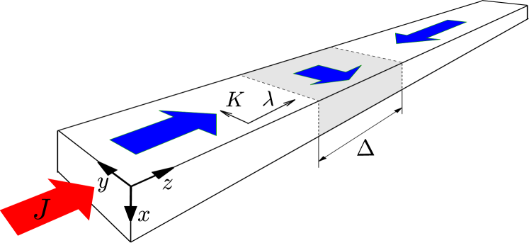
Figure 1: (color online) A schematic view of a current-driven domain wall in a ferromagnetic wire. The DW width is $\Delta$.

The schematic view of a domain wall in a narrow ferromagnetic wire is shown in Fig. 1. These DWs are characterized by their width $\Delta$ which is mainly determined by exchange interaction and anisotropy along the wire $\lambda$. Another important quantity is the transverse anisotropy across the wire $K$, which governs the pinning of the transverse component of the DW magnetization. When no current is applied to the wire it leads to two degenerate positions of the transverse magnetization component of the wall: as shown in Fig. 1 and anti-parallel to it.

To describe the dynamics of DW in a thin wire we derived the effective equations of motion from generalized Landau-Lifshitz-GilbertLi and Zhang (2004); Thiaville et al. (2005) (LLG) equation with the current $J$,

$$\dot{\mathbf{S}}=\mathbf{S}\times\mathbf{H}_{eff}-J\frac{\partial\mathbf{S}}{\partial z}+\beta J\mathbf{S}\times\frac{\partial\mathbf{S}}{\partial z}+\alpha\mathbf{S}\times\dot{\mathbf{S}},$$ (1)

where $\mathbf{S}$ is magnetization unit vector, $\mathbf{H}_{eff}=\delta\mathcal{H}/\delta\mathbf{S}$ is the effective magnetic field given by the Hamiltonian $\mathcal{H}$ of the system, $\beta$ is non-adiabatic spin torque constant, and $\alpha$ is Gilbert damping constant. The derivation of the effective equations of motion is based on the fact that in thin ferromagnetic wires the static DWs are rigid topologically constrained spin-textures. Therefore, for not too strong drive, their dynamics can be described in terms of only a few collective coordinates associated with the DW degrees of freedom. Tretiakov et al. (2008); *Clarke08 In very thin wires, there are two collective coordinates corresponding to two softest modes of the DW motion: the DW position along the wire $z_{0}$ and the magnetization angle $\phi$ in the DW around the wire axis. All other degrees of freedom are gapped by strong anisotropic energy along the wire.

By applying the orthogonality condition to LLG, one can obtain the equations of motion for the two DW softest modes, $z_{0}(t)$ and $\phi(t)$,Tretiakov and Ar. Abanov (2010)

$$\dot{z}_{0} = AJ+B[J-j_{c}\sin(2\phi)],$$ (2)

$$\dot{\phi} = C[J-j_{c}\sin(2\phi)],$$ (3)

where $J(t)$ is a time-dependent current. The coefficients $A$, $B$, $C$, and critical current $j_{c}$ can be evaluated for a particular model in terms of $\alpha$, $\beta$ and other microscopic parameters. Following Ref. Tretiakov and Ar. Abanov, 2010, for the model with Dzyaloshinskii-Moriya interaction (DMI) one can find $A=\beta/\alpha$, $B=(\alpha-\beta)(1+\alpha\Gamma\Delta)/[\alpha(1+\alpha^{2})]$, $C=(\alpha-\beta)\Delta/[(1+\alpha^{2})\Delta_{0}^{2}]$, and $j_{c}=(\alpha K\Delta/\left|\alpha-\beta\right|)[\pi\Gamma\Delta/\sinh(\pi\Gamma\Delta)]$, where $J_{\rm{ex}}$ is exchange constant, $D$ is DMI constant, and $\Gamma=D/J_{\rm{ex}}$. Also, $\Delta=\Delta_{0}/\sqrt{1-\Gamma^{2}\Delta_{0}^{2}}$ where $\Delta_{0}$ is the DW width in the absence of DMI.

Alternatively, Eqs. (2) and (3) can be obtained in a more general framework by means of symmetry arguments. We note that because of the translational invariance $\dot{z}_{0}$ and $\dot{\phi}$ cannot depend on $z_{0}$. Furthermore, to the first order in small transverse anisotropy $K$, $\dot{\phi}$ and $\dot{z}_{0}$ are proportional to the first harmonic $\sin(2\phi)$. Then the expansion in small current $J$ up to a linear in $J$ order gives Eqs. (2) and (3). In this case the coefficients $A$, $B$, $C$, and $j_{c}$ have to be determined directly from experimental measurements. Yang et al. (2009); Liu

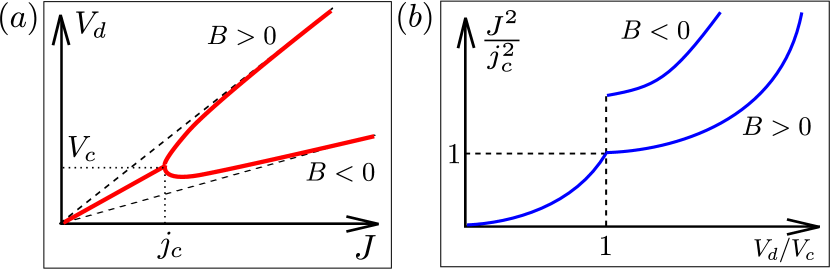
Figure 2: (color online) DW motion characteristics for dc currents. (a) Drift velocity $V_{d}$ of DW as a function of current $J$ for $B>0$ and $B<0$, see Eq. (2). The slope at $J<j_{c}$ is given by $A$, whereas at $J\gg j_{c}$ it is $A+B$. (b) Power of Ohmic losses $p_{\rm{dc}}(V_{d}/V_{c})=J^{2}/j_{c}^{2}$ as a function of drift velocity $V_{d}$. For $B<0$ the power has a discontinuity at $V_{d}/V_{c}=1$.

For the dc current applied to the wire the DW dynamics governed by Eqs. (2) and (3) can be obtained explicitly.Tretiakov and Ar. Abanov (2010) For $J<j_{c}$ and $A\neq 0$ the DW only moves along the wire and is tilted on angle $\phi_{0}$ from the transverse-anisotropy easy axis given by condition $\sin(2\phi_{0})=J/j_{c}$. The drift velocity is $V_{d}=\langle\dot{z}_{0}(J)\rangle=AJ$, see Eq. (2). Therefore, the linear slope of $V_{d}(J)$ below $j_{c}$ gives constant $A$, see Fig. 2 (a). The value of $j_{c}$ is determined as the endpoint of this linear regime. At $J=j_{c}$ the magnetization angle becomes perpendicular to the easy axis, $\phi_{0}=\pi/2$. For $J>j_{c}$ the DW both moves and rotates, and Eqs. (2) and (3) give $V_{d}=AJ+B\sqrt{J^{2}-j_{c}^{2}}$, so that the slope of $V_{d}(J)$ at large $J$ gives $A+B$.

Power optimization. The largest losses in the nanowire with a DW are the Ohmic losses of the current. In general, the influence of the DW on the resistance is negligible and therefore we can assume that the resistance of the wire is constant with time. Then the time-averaged power of Ohmic losses is proportional to $\langle J^{2}(t)\rangle$. Since the resistance is almost constant, in this paper we will calculate $P=\langle J^{2}(t)\rangle$ and loosely call it the power of Ohmic losses. Our goal is to minimize the Ohmic losses while keeping the DW moving with a given constant drift velocity.

For the following it will be convenient to introduce the dimensionless variables for time, drift velocity, current, power, and the ratio of slopes of $V_{d}(J)$ at large and small currents,

$$\tau=Cj_{c}t,\quad v_{d}=\frac{V_{d}}{V_{c}},\quad j=\frac{J}{j_{c}},\quad p=\frac{\mathcal{P}}{j_{c}^{2}},\quad a=\frac{A+B}{A}.$$ (4)

Although we note that in the special case of $\alpha=\beta$, it can be shown that $C=B=0$ and one cannot use dimensionless variables (4). However, in this case the DW dynamics is trivial: Barnes and Maekawa (2005) the DW does not rotate $\phi=0,\pi$ and moves with the velocity $\dot{z}_{0}=J$.

First, we consider the case of dc current and the power as a function of drift velocity. For $v_{d}<1$ we find $p_{\rm{dc}}=v_{d}^{2}$. For currents above $j_{c}$ the power $p_{\rm{dc}}(v_{d})=j^{2}$ is given in terms of drift velocity $v_{d}=j+(B/A)\sqrt{j^{2}-1}$ as shown in Fig. 2 (b). The power is quadratic in $v_{d}$, and for $B<0$ it has a discontinuity at $v_{d}=1$.

In general, the DW motion has some period $T$ and current $j(\tau)$ must be a periodic function with the same $T$ to minimize the Ohmic losses. Measuring the angle from the hard axis instead of easy axis and scaling it by 2, i.e, $2\phi=\theta-\pi/2$, we can write the dimensionless current drift velocity as Tretiakov, Liu, and Ar. Abanov

$$j(\tau)=\dot{\theta}/2-\cos\theta,\quad v_{d}=\frac{a}{2}\langle\dot{\theta}\rangle-\langle\cos\theta\rangle,$$ (5)

where $\dot{\theta}=\partial\theta/\partial\tau$.

To minimize the power of Ohmic losses we need to find the minimum of $\langle j^{2}(\tau)\rangle$ at fixed $v_{d}$,

$$\overline{p}=\left\langle(\dot{\theta}/2-\cos\theta)^{2}-2\rho(a\dot{\theta}/2-\cos\theta-v_{d})\right\rangle,$$ (6)

where we use a Lagrange multiplier $2\rho$ to account for the constraint given by $v_{d}$ from Eq. (5). Power (6) can be considered as an effective action for a particle in a periodic potential $U$, and its minimization gives the equation of motion $\ddot{\theta}/2=-\partial U/\partial\theta$ which in turn can be reduced to

$$\dot{\theta}=\pm 2\sqrt{d-U(\theta,\rho)},\quad U(\theta,\rho)=-\cos^{2}\theta-2\rho\cos\theta.$$ (7)

where $d$ is an arbitrary constant. Since changing $\rho\to-\rho$ in $U$ of Eq. (7) is equivalent to changing $\theta\to\pi+\theta$, below we can consider only positive $\rho$.

Eq. (7) shows that there are two different regimes: 1) the bounded regime where $d<\rm{max}[U(\theta,\rho)]$ in which case $\theta$ is bounded, and the particle oscillates in potential well $U(\theta)$, see inset of Fig. 3 (a); and 2) the rotational regime where $d>\rm{max}[U(\theta,\rho)]$ with freely rotating magnetization in the DW.

In the bounded regime the particle moves between the two turning points $-\theta_{0}$ and $\theta_{0}$ given by $d=U(\pm\theta_{0},\rho)$. Since $\theta$ is a bounded function $\langle\dot{\theta}\rangle=0$ and $v_{d}=-\langle\cos\theta\rangle$. One can showTretiakov, Liu, and Ar. Abanov that in this regime the power of Ohmic losses is minimal for dc current, i.e., $\overline{p}=v_{d}^{2}$.

In the rotational regime the term in Eq. (5) with $\langle\dot{\theta}\rangle$ should be kept because $\theta$ is not bounded. The equation of motion is the same as for a nonlinear oscillator.Tretiakov, Liu, and Ar. Abanov Using the minimization condition $\partial\overline{p}/\partial\rho|_{v_{d}}=0$ one finds

$$\int_{-\pi}^{\pi}\!\sqrt{d-U(\theta,\rho)}d\theta=2\pi a\rho.$$ (8)

This equation defines the relationship between $d$ and $\rho$.

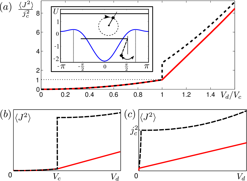
Figure 3: (color online) (a) Minimal power of Ohmic losses $\overline{p}=\langle J^{2}\rangle/j^{2}_{c}$ as a function of drift velocity $V_{d}$ shown by solid line for $a=0.5$. The dashed line depicts $\overline{p}$ for dc current. The inset shows the potential $U(\theta)$ in which a “particle” is moving in the bounded (pendulum-like) and unbounded (rotational) regimes. A sketch of $\langle J^{2}\rangle(V_{d})$ shown by solid line in (b) for $\beta\gg\alpha$ ($a\ll 1$) and (c) for $\beta\ll\alpha$ ($a\gg 1$).

The results for the minimal power of Ohmic losses $\overline{p}(v_{d})$ are presented in Fig. 3. For $a>1$ there is a critical velocity $v_{\rm{rc}}<1$, such that at $v_{d}<v_{\rm{rc}}$ the power of Ohmic losses is $\overline{p}=v_{d}^{2}=p_{\rm{dc}}$. Above $v_{\rm{rc}}$ one can minimize the Ohmic losses by moving DW with resonant current pulses. Right above $v_{\rm{rc}}$ there is a certain range of $v_{d}$ where $\overline{p}=2\rho_{0}v_{d}-\rho_{0}^{2}$ with $\rho_{0}(a)<1$ given by Eq. (8) with $d=\rho^{2}$. The critical velocity is found as $v_{\rm{rc}}=\rho_{0}(a)$. For $a<1$, see e.g. Fig. 3 (a), we find that $v_{\rm{rc}}=1$, whereas at $v_{d}>1$ minimal power $\overline{p}$ is significantly lower than $p_{\rm{dc}}$. Immediately above $v_{d}=1$ we find that there is a range of $v_{d}$ where $\overline{p}$ is linear in $v_{d}$. At large $v_{d}$ the minimal power is always smaller than $p_{\rm{dc}}$, the difference between them then approaches $p_{\rm{dc}}-\overline{p}=(1-1/a)^{2}/2$.

We note that even in the limiting cases of the systems with weak ($\beta\ll\alpha$) or strong ($\beta\gg\alpha$) non-adiabatic spin transfer torque, see Fig. 3 (b) and (c), where the power of Ohmic losses is high for dc currents, the optimized ac current gives dramatic reduction in heating power thus greatly expanding the range of materials which can be used for spintronic devices. Allwood et al. (2005); Parkin, Hayashi, and Thomas (2008) We also note that DMI suppresses critical current $j_{c}$ and affects parameter $a$.

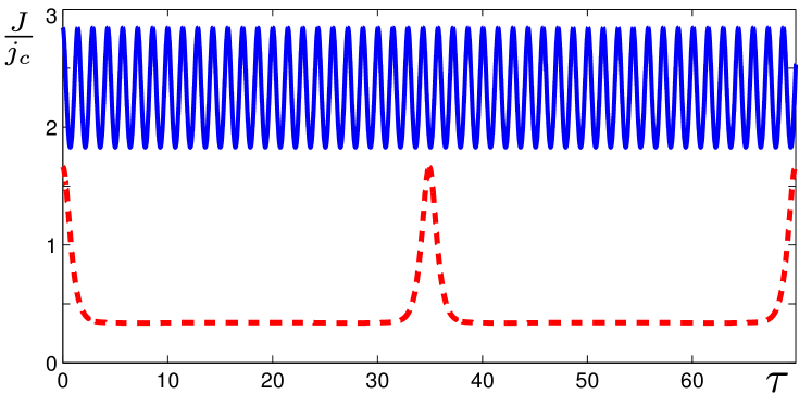
Figure 4: (color online) Resonant time-dependent current $J(\tau)$ with $\tau=Cj_{c}t$ for drift velocities $v_{d}=0.5$ (dashed line) and $v_{d}=4.5$ (solid line) for $a=2$.

For $v_{d}<v_{\rm{rc}}$ the optimal current coincides with the dc current, above $v_{\rm{rc}}$ the resonant current $j(t)$ is plotted in Fig. 4 for $a=2$ and two different velocities $v_{d}$. At $v_{d}>v_{\rm{rc}}$ the current’s maximum $j_{\rm{max}}$ increases from $2-v_{\rm{rc}}$ at small enough $v_{d}\lesssim 1$ up to $j_{\rm{max}}\approx v_{d}/a$ at $v_{d}\gg 1$. The current’s minimum increases monotonically from small positive values $j_{\rm{min}}=v_{\rm{rc}}$ at $v_{d}\sim 1$ up to $j_{\rm{min}}=j_{\rm{max}}-2|1-a|/a$ at $v_{d}\gg 1$. At $v_{d}\lesssim 1$ (for $a>1$) the time between the current picks decreases with increasing velocity as $T\simeq(\pi a-2\arcsin v_{\rm{rc}})/(v_{d}-v_{\rm{rc}})$, whereas the pick’s width is given by $\approx 1.3/\sqrt{(1-v_{\rm{rc}})}$. Therefore, at small $v_{d}-v_{\rm{rc}}$ the picks are widely separated, then as $v_{d}$ increases the time between the picks decreases. At $v_{d}\gg 1$ the optimal current has a large constant component and small-amplitude ac modulations on top of it.

Conclusions. We have studied the current driven DW dynamics in thin ferromagnetic wires. The ultimate lower bound for the Ohmic losses in the wire has been found for any DW drift velocity $V_{d}$. We have obtained the explicit time-dependence of the current which minimizes the Ohmic losses. We believe that the use of these resonant current pulses instead of dc current can help to dramatically reduce heating of the wire for any $V_{d}$.

We thank Jairo Sinova for valuable discussions. This work was supported by the NSF Grant No. 0757992 and Welch Foundation (A-1678).

References

- Parkin, Hayashi, and Thomas (2008) S. S. P. Parkin, M. Hayashi, and L. Thomas, Science 320, 190 (2008).
- Hayashi et al. (2008) M. Hayashi, L. Thomas, R. Moriya, C. Rettner, and S. S. P. Parkin, Science 320, 209 (2008).
- Allwood et al. (2002) D. A. Allwood, G. Xiong, M. D. Cooke, C. C. Faulkner, D. Atkinson, N. Vernier, and R. P. Cowburn, Science 296, 2003 (2002).
- Allwood et al. (2005) D. A. Allwood, G. Xiong, C. C. Faulkner, D. Atkinson, D. Petit, and R. P. Cowburn, Science 309, 1688 (2005).
- Ono et al. (1999) T. Ono, H. Miyajima, K. Shigeto, K. Mibu, N. Hosoito, and T. Shinjo, Science 284, 468 (1999).
- Yamaguchi et al. (2004) A. Yamaguchi, T. Ono, S. Nasu, K. Miyake, K. Mibu, and T. Shinjo, Phys. Rev. Lett. 92, 077205 (2004).
- (7) O. A. Tretiakov, Y. Liu, and Ar. Abanov, Phys. Rev. Lett., in press; arXiv:1006.0725.
- Li and Zhang (2004) Z. Li and S. Zhang, Phys. Rev. Lett. 92, 207203 (2004).
- Thiaville et al. (2005) A. Thiaville et al., Europhys. Lett. 69, 990 (2005).
- Tretiakov et al. (2008) O. A. Tretiakov, D. Clarke, G.-W. Chern, Y. B. Bazaliy, and O. Tchernyshyov, Phys. Rev. Lett. 100, 127204 (2008).
- Clarke et al. (2008) D. J. Clarke, O. A. Tretiakov, G.-W. Chern, Y. B. Bazaliy, and O. Tchernyshyov, Phys. Rev. B 78, 134412 (2008).
- Tretiakov and Ar. Abanov (2010) O. A. Tretiakov and Ar. Abanov, Phys. Rev. Lett. 105, 157201 (2010).
- Yang et al. (2009) S. A. Yang, G. S. D. Beach, C. Knutson, D. Xiao, Q. Niu, M. Tsoi, and J. L. Erskine, Phys. Rev. Lett. 102, 067201 (2009).
- (14) Y. Liu, O. Tretiakov, and Ar. Abanov, (unpublished).
- Barnes and Maekawa (2005) S. E. Barnes and S. Maekawa, Phys. Rev. Lett. 95, 107204 (2005).