Relativistic heat conduction: the kinetic theory approach and comparison with Marle’s model

Abstract

In order to close the set of relativistic hydrodynamic equations, constitutive relations for the dissipative fluxes are required. In this work we outline the calculation of the corresponding closure for the heat flux in terms of the gradients of the independent scalar state variables: number density and temperature. The results are compared with the ones obtained using Marle’s approximation in which a relativistic correction factor is included for the relaxation time parameter. It is shown how including such correction this BGK-like model yields good results in the relativistic case and not only in the non-relativistic limit as was previously found by other authors.

I Introduction

The interest in relativistic non-equilibrium thermodynamics has grown recently, mostly due to recent experiments as well as new ideas in theoretical modeling Kodama ; Azwinndini1 ; Azwinndini2 ; Policastro . Most works dealing with applications of the theory do not refer to the corresponding system of transport equations including dissipation to first order in the gradients. This is principally due to the fact that for decades such system has been thought to predict unphysical dynamics in the fluid Hiscock . However, it was recently pointed out that when kinetic theory is used to formulate the constitutive equations that complete such set, instead of phenomenological arguments, the system of transport equations is free of instabilities and shows no causality issues in the linear regime PA2009 .

Relativistic kinetic theory to first order in the gradients has been vastly explored by previous authors Israel ; deGroot ; kremer . In those works the purely relativistic term that appears in the closure for the heat flux is included in a generalized thermal force with one transport coefficient i.e. a relativistic thermal conductivity. However, the system of transport equations constitutes a set of five balance equations and needs to be eventually expressed in terms of only five state variables. In the usual representation, these variables are the number density $n$, the hydrodynamic four velocity $\mathcal{U}^{\nu}$, which only has three independent components, and temperature $T$. Because of this, constitutive equations for the dissipative fluxes in terms of gradients of those quantities are required to close the system. The aim of this work is to show the highlights of the calculation of the heat flux from the complete Boltzmann equation using the Chapman-Enskog approximation within the $n,\,\mathcal{U}^{\nu},\,T$ representation. The details and further analysis of this calculation can be found in Ref. aa2010 . In order to perform this task we consider the density and temperature gradients as independent forces and write two uncoupled integral equations. The coefficients involved in the constitutive relation are calculated and plotted for a constant cross section model. Here, we also compare the results with those found in previous works using a BGK-like approximation PA2009 ; aip-proceedings2009 . In order to make such comparison, we adjust the parameter included in Marle’s kernel by a relativistic factor arising from the structure of the kinetic equation. We further show that when this factor is taken into account, the deviation from the exact values are as significative as in the non-relativistic case.

The rest of this work is organized as follows. In the second section some basic elements of relativistic kinetic theory are briefly reviewed including the Chapman-Enskog expansion for the solution of the Boltzmann equation. In the third section an outline of the calculation of the heat flux using two independent forces is shown. The results for the transport coefficients are compared to the values obtained in the BGK approximation in section four and some final remarks and conclusions are included in the last section.

II Relativistic kinetic theory

In the kinetic theory of gases, the evolution of the distribution function of a a dilute gas is given by the Boltzmann equation. If the temperature $T$ of such gas is high enough such that the relativistic parameter $z=kT/mc^{2}$, where $m$ is the rest mass of the particles, $c$ the speed of light and $k$ Boltzmann’s constant, is not negligible, the non-relativistic description is not appropriate. Instead, relativistic kinetic theory (RKT) constitutes a more accurate framework. In RKT the fact that the speed of the molecules can be close to the speed of light is taken into account. The evolution of the distribution function is then given by the special relativistic Boltzmann equation lichnerowicz

$$v^{\alpha}f_{,\alpha}=J(f\,f^{\prime}),$$ (1)

where $v^{\alpha}=\gamma\left(\omega^{\ell},c\right)$ is the molecular four-velocity, $\gamma$ being Lorentz factor , and $J(f,f^{\prime})$ is the collision kernel kremer

$$J\left(f\,f^{\prime}\right)=\int\int\left[f\,^{\prime}f_{1}\,^{\prime}-f\,f_{1}\right]\mathcal{F}\sigma\left(\Omega\right)d\Omega dv_{1}^{*}$$

In the previous equation $\mathcal{F}$ the invariant flux and $\sigma\left(\Omega\right)d\Omega$ is the differential cross section kremer . The system here considered is a dilute, single component, neutral, non-degenerate, inert gas. The local variables, number density $n$, hydrodynamic four-velocity $u^{\nu}$ and internal energy density $e$, are defined as

$$n=\int f\gamma dv^{*},$$ (2)

$$nu^{\nu}=\int fv^{\nu}dv^{*},$$ (3)

$$ne=mc^{2}\int f\gamma^{2}dv^{*}.$$ (4)

respectively. The local equilibrium distribution function, which is the solution of the homogeneous Boltzmann equation, in the relativistic case is given by Ref. Juttner

$$f^{(0)}=\frac{n}{4\pi c^{3}}\frac{1}{zK_{2}\left(\frac{1}{z}\right)}\exp^{\frac{u^{\nu}v_{\nu}}{zc^{2}}}$$ (5)

where $K_{n}(x)$ is the modified Bessel function of the second kind. As shown in Ref. AAL2010 , the heat flux can be calculated as the average of the chaotic kinetic energy, that is

$$q^{\mu}=mc^{2}h_{\nu}^{\mu}\int\gamma v^{\nu}fd^{*}v$$ (6)

The chaotic velocity corresponds to the velocity measured in a local comoving frame. Thus, one can replace the invariant $u^{\nu}v_{\nu}$ in Eq. (5) by its value in the local comoving frame, that is $u^{\nu}v_{\nu}=-c^{2}\gamma$. In this context the total energy and momentum fluxes for an arbitrary observer are given by the Lorentz transformed dissipative fluxes as calculated in the local comoving frame. This argument is clearly discussed in Refs. aa2010 ; AAL2010 .

In order to calculate the heat flux, given in Eq. (6), one does not need an explicit solution to the Boltzmann equation. Using Hilbert’s method one can obtain a good approximation to the integral in Eq. (6). Following the prescription of such method, the velocity distribution function is written as $f=f^{(0)}+f^{(1)}$ where $f^{\left(1\right)}$ is considered to be a first order correction in the gradients of the state variables. Also, in order to associate the local variables to the equilibrium state, the following subsidiary conditions need to be imposed

$$\int f^{(1)}\left(\begin{array}[]{c}\gamma^{2}\\ v^{\nu}\end{array}\right)dv^{*}=0.$$ (9)

Under these hypotheses, the linearized relativistic Boltzmann equation, obtained by substituting $f$ in Eq. (1) and considering only linear deviations from local equilibrium, reads

$$v^{\alpha}f_{,\alpha}^{(0)}=f^{(0)}\mathbin{C}(\phi)$$ (10)

where

$$\mathbin{C}\left(\phi\right)=\int\int\left\{\phi^{\prime}_{1}+\phi^{\prime}-\phi_{1}-\phi\right\}f_{1}^{\left(0\right)}\mathcal{F}\sigma\left(\Omega\right)d\Omega dv_{1}^{*},$$

is the linearized collision kernel. Substituting $f^{(0)}$ on the left hand side and using the identity $v^{\alpha}A_{,\alpha}=h^{\mu\nu}v_{\nu}A_{,\mu}-\frac{\mathcal{U}^{\mu}\mathcal{U}^{\nu}}{c^{2}}v_{\nu}A_{,\mu}$ Eq. (10) yields

$$v^{\alpha}f_{,\alpha}^{(0)} =f^{(0)}h^{\mu\nu}v_{\nu}\left(\frac{n_{,\mu}}{n}-\frac{T_{,\mu}}{T}\left[1+\frac{u^{\beta}v_{\beta}}{zc^{2}}+\frac{1}{2z}\left(\frac{K_{1}(\frac{1}{z})+K_{3}(\frac{1}{z})}{K_{2}(\frac{1}{z})}\right)\right]+\frac{v_{\beta}u_{;\mu}^{\beta}}{zc^{2}}\right)$$ (11)

$$+f^{(0)}\gamma c\left(\frac{\dot{n}}{n}-\frac{\dot{T}}{T}\left[1+\frac{u^{\beta}v_{\beta}}{zc^{2}}+\frac{1}{2z}\left(\frac{K_{1}(\frac{1}{z})+K_{3}(\frac{1}{z})}{K_{2}(\frac{1}{z})}\right)\right]+\frac{v^{\beta}\dot{u}_{\beta}}{zc^{2}}\right).$$

Notice that the first line in Eq. (11) only includes the spatial components, since in the comoving frame $h^{\mu 4}=0$ while the time derivatives are isolated in the second line which we have simplified using that

$$\frac{u^{\mu}u^{\nu}}{c^{2}}v_{\nu}=-u^{\mu}\gamma\delta_{\mu}^{4}$$

This separation between temporal and spatial parts is particularly useful since for the Chapman-Enskog solution to first order in the gradients to exist, the previous order equations have to be satisfied. Because of this, the relativistic Euler equations namely,

$$\dot{n}=-nu_{;\alpha}^{\alpha},$$

$$\dot{u}=-\left(\frac{ne}{c^{2}}+\frac{p}{c^{2}}\right)^{-1}p_{,\mu}h_{\beta}^{\mu},$$ (12)

$$\dot{T}=-\frac{T\beta}{nC_{n}k}u_{;\alpha}^{\alpha},$$

are substituted in the expression in Eq. (11) such that only spatial gradients appear in it. Also, since the momentum balance equation is in terms of the gradient of the hydrostatic pressure, we introduce in it the relation

$$p_{,\mu}=\left(\frac{\partial p}{\partial n}\right)n_{,\mu}+\left(\frac{\partial p}{\partial T}\right)T_{,\mu}.$$ (13)

in order to be consistent with our representation. After Euler Eqs. (12), are introduced in Eq. (11) and using the equation state for an ideal gas $p=nkT$, we can write

$$v^{\beta}h_{\beta}^{\alpha}\left\{\left(1-\gamma\frac{K_{2}(\frac{1}{z})}{K_{3}(\frac{1}{z})}\right)\frac{n_{,\alpha}}{n}+\frac{T_{,\alpha}}{T}\left(1+\frac{\gamma}{z}-\gamma\frac{K_{2}(\frac{1}{z})}{K_{3}(\frac{1}{z})}-\frac{K_{3}(\frac{1}{z})}{zK_{2}(\frac{1}{z})}\right)\right\}=\mathbin{C}(\phi).$$ (14)

Since in this work we are only interested in the heat flux, we have ignored the term proportional to $u_{;\alpha}^{\beta}$ in Eq. (14) due to Curie’s principle.

Following Hilbert’s method, the general solution for the integral equation (14) is given by the sum of a particular solution and a linear combination of the collision invariants as solutions to the homogeneous equation. That is

$$\phi=\mathcal{A}(\gamma)v^{\alpha}h_{\beta}^{\alpha}\frac{T_{,\alpha}}{T}+\mathcal{B}(\gamma)v^{\alpha}h_{\beta}^{\alpha}\frac{n_{,\alpha}}{n}+\alpha+\tilde{\alpha}_{\nu}v^{\nu}$$ (15)

where $\mathcal{A}(\gamma)$ and $\mathcal{B}(\gamma)$ are functions of $\gamma$ and the local variables $n,\vec{v},T$ while $\alpha$ and $\tilde{\alpha}_{\nu}$ are constants. By imposing the subsidiary conditions, required for the uniqueness of the solution, Eq. (9), $\phi$ can be rewritten as

$$\phi=\mathcal{A}(\gamma)v^{\beta}h_{\beta}^{\alpha}\frac{T_{,\alpha}}{T}+\mathcal{B}(\gamma)v^{\beta}h_{\beta}^{\alpha}\frac{n_{,\alpha}}{n}.$$ (16)

The coefficients $\mathcal{A}(\gamma)$ and $\mathcal{B}(\gamma)$ are further expressed in terms of orthogonal polynomials in the form

$$\mathcal{A}(\gamma)=\sum_{n=0}^{\infty}a_{n}\mathcal{L}_{n}(\gamma),$$

$$\mathcal{B}(\gamma)=\sum_{n=0}^{\infty}b_{n}\mathcal{L}_{n}(\gamma),$$

with $\mathcal{L}_{n}(\gamma)=\sum_{k=0}^{n}\alpha_{kn}\gamma^{k}$. The elements of this set satisfy the orthogonality condition

$$\int\mathcal{L}_{n}(\gamma)\mathcal{L}_{m}(\gamma)\exp^{-\frac{\gamma}{z}}(\gamma^{2}-1)^{3/2}d\gamma=\delta_{nm},$$

More details on these polynomials can be consulted in Refs. kremer ; aa2010 . Direct substitution of coefficients $\mathcal{A}(\gamma)$ and $\mathcal{B}(\gamma)$ in the solution (16) leads us to the expression

$$\phi=h_{\beta}^{\alpha}\sum_{n=0}^{\infty}a_{n}\mathcal{L}_{n}(\gamma)v^{\beta}{\frac{T_{,\alpha}}{T}}+h_{\beta}^{\alpha}\sum_{n=0}^{\infty}b_{n}\mathcal{L}_{n}(\gamma)v^{\beta}{\frac{n_{,\alpha}}{n}},$$ (17)

It is worthwhile pointing out that the first-order approximation for the distribution function is obtained here in terms of the density and temperature gradients as was already discussed in PA2009 ; aa2010 . This is because of the chosen representation in which $n$ and $T$ are considered independent state variables. Thus, when the heat flux is calculated from the distribution function, the term proportional to the temperature gradient will lead us to a Fourier-like law, while the term proportional to the density gradient is a purely relativistic contribution. The latter has no non-relativistic counterpart since the corresponding term in Eq. (14) vanishes in such limit.

Substituting the proposed solution $\phi$ in the linearized Boltzmann equation (14) leads to an integral equation

$$v^{\beta}h_{\beta}^{\alpha}\left\{\left(1-\gamma\frac{K_{2}(\frac{1}{z})}{K_{3}(\frac{1}{z})}\right)\frac{n_{,\alpha}}{n}+\frac{T_{,\alpha}}{T}\left(1+\frac{\gamma}{z}-\gamma\frac{K_{2}(\frac{1}{z})}{K_{3}(\frac{1}{z})}-\frac{K_{3}(\frac{1}{z})}{zK_{2(\frac{1}{z})}}\right)\right\}=\mathbin{C}(\phi).$$

which can be separated into two independent equations as follows

$$v^{\beta}h_{\beta}^{\alpha}\left\{1+\frac{\gamma}{z}-\gamma\frac{K_{2}(\frac{1}{z})}{K_{3}(\frac{1}{z})}-\frac{K_{3}(\frac{1}{z})}{zK_{2}(\frac{1}{z})}\right\}=h_{\beta}^{\alpha}\sum_{n=1}^{\infty}a_{n}\mathbin{C}(\mathcal{L}_{n}(\gamma)v^{\beta})$$

$$v^{\beta}h_{\beta}^{\alpha}\left\{1-\gamma\frac{K_{2}(\frac{1}{z})}{K_{3}(\frac{1}{z})}\right\}=h_{\beta}^{\alpha}\sum_{n=1}^{\infty}b_{n}\mathbin{C}(\mathcal{L}_{n}(\gamma)v^{\beta}).$$

As mentioned above, the explicit complete solution for $f^{\left(1\right)}$ is not required in order to calculate the heat flux. As will be shown in the next section only one term in the infinite sums appearing in the previous equations is enough in order to get a good approximation for $q^{\mu}$.

III Heat flux

The heat flux is physically the average of a chaotic energy flux. Because of this, it is calculated in the local comoving frame, as is clearly stated in Eq. (6). Substituting $f^{(1)}=f^{(0)}\phi$ with $\phi$ given by Eq. (17) in Eq. (6) yields

$$q^{\mu}=\frac{nm}{4\pi czK_{2}(\frac{1}{z})}\left[I_{a}^{\mu}+I_{b}^{\mu}\right],$$ (18)

where the integrals in the bracket are given by

$$I_{a}^{\nu}=\int\left[\mathcal{A}(\gamma)v_{k}\frac{T^{,k}}{T}\right]\gamma v^{\nu}\exp^{-\frac{\gamma}{z}}\sqrt{\gamma^{2}-1}d\gamma,$$ (19)

$$I_{b}^{\nu}=\int\left[\mathcal{B}(\gamma)v_{k}\frac{n^{,k}}{n}\right]\gamma v^{\nu}\exp^{-\frac{\gamma}{z}}\sqrt{\gamma^{2}-1}d\gamma.$$ (20)

In Ref. aa2010 it is shown how, of all coefficients $a_{n}$ and $b_{n}$ in Eqs. (19) and (20), only one of each is required in order to obtain a good first approximation to $I_{a}^{\nu}$ and $I_{b}^{\nu}$. After a cumbersome calculation, which can be found to some detail in Ref. aa2010 , and assuming constant collisions cross-section (see kremer ) one obtains

$$q^{\mu}=-h^{\mu\alpha}\left[L_{T}\frac{T_{,\alpha}}{T}+L_{n}\frac{n_{,\alpha}}{n}\right],$$ (21)

where the transport coefficients $L_{T}$ and $L_{n}$ can be written as

$$L_{T}=\frac{3}{64}\frac{ckT}{\pi\sigma}f_{1}(z)\qquad L_{n}=\frac{3}{64}\frac{ckT}{\pi\sigma}f_{2}(z)$$ (22)

where

$$f_{1}(z)=\left(1-z\frac{K_{2}(\frac{1}{z})}{K_{3}(\frac{1}{z})}\right)\frac{\left(K_{2}\left(\frac{1}{z}\right)\left[\frac{1}{z}+5\mathcal{G}\left(\frac{1}{z}\right)-\frac{1}{z}\mathcal{G}\left(\frac{1}{z}\right)^{2}\right]\right)^{2}}{z^{4}\left(\frac{5}{z}K_{3}\left(\frac{2}{z}\right)+\left(\frac{1}{z^{2}}+2\right)K_{2}\left(\frac{2}{z}\right)\right)}$$ (23)

$$f_{2}(z)=-\frac{K_{2}\left(\frac{1}{z}\right)\left(K_{2}\left(\frac{1}{z}\right)\left[\frac{1}{z}+5\mathcal{G}\left(\frac{1}{z}\right)-\frac{1}{z}\mathcal{G}\left(\frac{1}{z}\right)^{2}\right]\right)^{2}}{z^{3}K_{3}\left(\frac{1}{z}\right)\left(\frac{5}{z}K_{3}\left(\frac{2}{z}\right)+\left(\frac{1}{z^{2}}+2\right)K_{2}\left(\frac{2}{z}\right)\right)}.$$ (24)

and $\mathcal{G}(1/z)=K_{3}(1/z)/K_{2}(1/z)$. In order to compare these results with the ones obtained in the relaxation time approximation we will explore Marle’s model in the next section and find appropriate expressions for the functions $f_{1}(z)$ and $f_{2}(z)$ in such context.

IV Comparison with the BGK approximation

The BGK approximation consists in replacing the right hand side of the Boltzmann equation with a simplified kernel in which all the details of the collisions are substituted by a parameter. The kinetic equation within relaxation models reads

$$v^{\alpha}f_{,\alpha}=-\mathcal{K}(f-f^{(0)}).$$ (25)

where the parameter $\mathcal{K}$ is assumed to be independent of $v^{\mu}$. The transport coefficients obtained using this method will have a strong dependence on this parameter. Thus, in order to compare the results obtained in the previous section using the complete kernel with the ones obtained with this model we need an approximation for the parameter $\mathcal{K}$.

To understand the role of this constant we follow the standard reasoning. We assume that the one particle distribution function does not depend on the spatial coordinates such that we can write

$$\gamma\frac{df}{dt}=-\mathcal{K}(f-f^{(0)})$$

from where one obtains

$$f(t)=\exp\left(-\frac{\mathcal{K}t}{\gamma}\right)\left[f(0)+\frac{\mathcal{K}}{\gamma}\int_{0}^{t}\exp\left(\frac{\mathcal{K}x}{\gamma}\right)f^{(0)}(x)dx\right]$$ (26)

Equation (26) motivates the association of the quantity $\gamma/\mathcal{K}$ with a characteristic relaxation time $\tau$. In the non-relativistic case, the analog to Eq. (26) leads to assuming $\tau\sim\mathcal{K}$. In Ref. kremer the $\gamma$ factor is not included in $\mathcal{K}$ which at the end leads to results for the thermal conductivity that deviate substantially from the complete solution value in the relativistic and ultra-relativistic scenarios. Only when $\gamma\to 1$, in the non-relativistic limit, the results are consistent.

Here we consider $\tau\sim\gamma/\mathcal{K}$ and propose a reasonable estimate for the parameter $\mathcal{K}$ from known characteristic times related to the collisions in the system. In non-relativistic kinetic theory, the time between collisions $\tau_{c}$ for hard-sphere particles of cross section $\sigma$ is given by

$$\tau_{c}=\frac{1}{4n\pi\sigma\langle g\rangle}$$

where $\langle g\rangle$ denotes the mean value of the relative velocity of two particles. Usually, the relaxation time $\tau$ appearing in BGK model, is considered proportional to $\tau_{c}$ and since $\langle g\rangle$ is of the order of the mean velocity $\langle v\rangle$ and/or the adiabatic sound speed $v_{s}=\sqrt{5kT/3m}$, we propose for this case

$$\frac{\gamma}{\mathcal{K}}=\frac{1}{4n\pi\sigma V(z)}$$ (27)

where $V(z)$ is the characteristic speed proportional to $\langle v\rangle$ or $v_{s}$. Finally to approximate $\mathcal{K}$ we propose

$$\frac{1}{\mathcal{K}}\sim\frac{1}{4n\pi\sigma V(z)\langle\gamma\rangle},$$ (28)

in analogy with the non-relativistic case.

Using Marle’s model, Sandoval et al. PA2009 obtained expressions for the transport coefficients which can be written in same fashion as Eq. (22) where the functions $f_{1}(z)$ and $f_{2}(z)$ are replaced by

$$f_{1M}(z)=\frac{16c}{3}\left(1-z\frac{K_{2}}{K_{3}}\right)\left\{\frac{1}{z}+5\mathcal{G}\left(\frac{1}{z}\right)-\frac{1}{z}\mathcal{G}\left(\frac{1}{z}\right)^{2}\right\}\frac{4n\pi\sigma}{\mathcal{K}}$$ (29)

$$f_{2M}(z)=-\frac{16c}{3}\frac{zK_{2}}{K_{3}}\left\{\frac{1}{z}+5\mathcal{G}\left(\frac{1}{z}\right)-\frac{1}{z}\mathcal{G}\left(\frac{1}{z}\right)^{2}\right\}\frac{4n\pi\sigma}{\mathcal{K}}.$$ (30)

where we have included the $M$’s subscript to indicate Marle’s model solution.

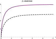
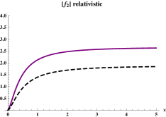
Figure 1: Relativistic coefficients $f_{1}$ and $f_{2}$. The continuous line for the complete kernel and the dashed line for Marle’s model including the $\gamma$ factor in the relaxation parameter.

The results of substituting expression (27) into (29) and (30) are shown in Fig. 1, where we have considered $V(s)=\sqrt{2}\langle v\rangle$. As can be clearly seen from the plot, the deviation of the approximated solution from the exact one is not as significant as without the $\gamma$ factor, which is shown in Fig. 2. Moreover, the difference between exact and approximated solutions when the $\gamma$ factor is taken into account is not grater than to the one obtained in the non-relativistic case which is shown in Fig. 3, for the sake of comparison.

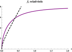
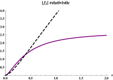
Figure 2: Relativistic coefficients $f_{1}$ and $f_{2}$. The continuous line for the complete kernel and the dashed line for Marle’s model without taking into account the $\gamma$ factor in the relaxation parameter.

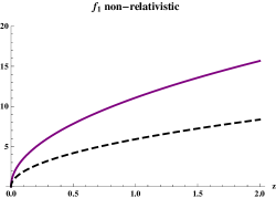
Figure 3: Non-relativistic case with the complete kernel (continuous line) and the BGK model (dashed line). Only the thermal conductivity factor $f_{1}$ is shown since $f_{2}$ corresponds to a purely relativistic correction.

With the information in hand, one can also infer the most reasonable expression for the characteristic velocity $V(z)$ with the help of both models. To accomplish this task, we write

$$\frac{1}{\mathcal{K}}\frac{L_{T}}{L_{MT}}=\frac{3}{64\pi\sigma nc}\frac{K_{2}\left(\frac{1}{z}\right)^{2}\left[\frac{1}{z}+5\mathcal{G}\left(\frac{1}{z}\right)-\frac{1}{z}\mathcal{G}\left(\frac{1}{z}\right)^{2}\right]}{z^{4}\left(\frac{5}{z}K_{3}\left(\frac{2}{z}\right)+\left(\frac{1}{z^{2}}+2\right)K_{2}\left(\frac{2}{z}\right)\right)}$$

and

$$\frac{1}{\mathcal{K}}\frac{L_{n}}{L_{Mn}}=\frac{3}{64\pi c\sigma n}\frac{K_{2}\left(\frac{1}{z}\right)^{2}\left[\frac{1}{z}+5\mathcal{G}\left(\frac{1}{z}\right)-\frac{1}{z}\mathcal{G}\left(\frac{1}{z}\right)^{2}\right]}{z^{4}\left(\frac{5}{z}K_{3}\left(\frac{2}{z}\right)+\left(\frac{1}{z^{2}}+2\right)K_{2}\left(\frac{2}{z}\right)\right)}$$

and consider the best approximation to $V(z)$ to be the one that makes both coefficients $L_{T}$’s or $L_{n}$’s match perfectly. The results are shown in Fig. 4 together with the characteristic velocity given by Eq. (28) and $v_{s}$. Note that $V_{c}\left(z\right)$ is the value one should give to the characteristic relative speed for the relaxation time model to match exactly the results obtained with the complete kernel.

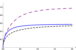
Figure 4: This plot shows a comparison of the different characteristic velocities $V_{c}(z)$ (long dashed line), $\langle v\rangle(z)$ (dashed line) and $v_{s}(z)$ (continuous line) .

V Final remarks

The relativistic hydrodynamic equations at the Navier-Stokes level need closure relations in order to constitute a complete set. In particular, the constitutive equation for the heat flux can be written in terms of the gradients of the temperature and the density when such quantities are considered independent state variables. The corresponding coupling coefficients have been calculated before assuming Marle’s model PA2009 ; aip-proceedings2009 . Here we outlined the procedure for the exact calculation, within Chapman-Enskog’s approximation, and compared the results in the case of constant cross-section collisions.

We re-analyzed Marle’s proposal as a relaxation model and found that the quantity related to a relaxation time is actually best approximated by $\langle\gamma\rangle/\mathcal{K}$. With this correction Marle’s model proves to be a good approximation not only in very mildly relativistic systems. Additionally we compare the different values that can be assigned to the characteristic microscopic velocity when approximating the value for $\mathcal{K}$ with the one inferred from the exact solution.

We finally wish to point out the similarity in structure of the second term in Eq. (21) with the Dufour effect. This is only in the sense that such relation implies the existence of a heat flux even in isothermic conditions due to a gradient in density. However, the coupling between heat and the density gradient in relativistic gases cannot be properly referred to as a cross effect since there is no reciprocal (diffusive) flux. The Dufour effect is the heat flux due to a diffusive force that appears in more than one component systems and has a conjugate effect called Soret effect. The role of the term here studied in the case of a binary mixture is still not clear and will be addressed in the future.

Acknowledgements: This work was partially supported by PROMEP grant UAM-PTC-142.

References

- (1) T. Kodama, T. Koide, G. S. Denicol, and P. Mota, Int.J.Mod.Phys.E 16, 763 (2007).
- (2) A. Muronga, Phys. Rev. C 76, 014909 (2007).
- (3) A. Muronga, Phys. Rev. C 76, 014910 (2007).
- (4) G. Policastro, JHEP 0209, 043 (2001).
- (5) W. A. Hiscock and L. Lindblom, Phys. Rev. D 31, 725 (1985).
- (6) A. Sandoval-Villalbazo, A. L. García-Perciante and L. S. García-Colin, Physica A 388, 3765 (2009).
- (7) W. Israel, J. Math. Phys 4, 1163 (1963).
- (8) S. R. de Groot, W. A. van Leeuwen and C. van der Wert, Relativistic Kinetic Theory (North Holland Publ. Co., Amsterdam,1980).
- (9) C. Cercignani and G. Kremer, The relativistic Boltzmann equation: Theory and applications (Cambridge University Press, UK, 1991).
- (10) A. L. García-Perciante and A. R. Méndez, arxiv:1009.6220v1 (2010).
- (11) A. Sandoval-Villalbazo, A. L. García-Perciante and L. S. García-Colin, Physics and Mathematics of Gravitation, in AIP Conf. Proc. 1122, Edited by Kunze, Mars, and Vazquez-Mozo, 388 (2009).
- (12) A. Lichnerowicz and R. Marrot, Compt. Rend. Acad. Sc. 210, 759 (1940).
- (13) F. Jüttner, Annalen der Physik 339, 856 (1911).
- (14) A. L. García-Perciante, A. Sandoval-Villalbazo and L. S. García-Colin, arXiv:1007.2815v1 (2010).