Quantifying the Imprecision of Accretion Theory and Implications for Multi-Epoch Observations of Protoplanetary Discs

Abstract

If accretion disc emission results from turbulent dissipation, then axisymmetric accretion theory must be used as a mean field theory: turbulent flows are at most axisymmetric only when suitably averaged. Spectral predictions therefore have an intrinsic imprecision that must be quantified to interpret the variability exhibited by a source observed at different epochs. We quantify contributions to the stochastic imprecision that come from azimuthal and radial averaging and show that the imprecision is minimized for a particular choice of radial averaging, which in turn, corresponds to an optimal spectral resolution of a telescope for a spatially unresolved source. If the optimal spectral resolution is less than that of the telescope then the data can be binned to compare to the theoretical prediction of minimum imprecision. Little stochastic variability is predicted at radii much larger than that at which the dominant eddy turnover time ($\sim$ orbit time) exceeds the time interval between observations; the epochs would then be sampling the same member of the stochastic ensemble. We discuss the application of these principles to protoplanetary discs for which there is presently a paucity of multi-epoch data but for which such data acquisition projects are underway.

1 Introduction

Accretion discs are ubiquitous in astrophysics, often forming around stars and compact objects where angular momentum would inhibit direct gravitational infall of the plasma onto the central object. A long standing theme of research in accretion theory has been to understand how how the discs transport angular momentum and remain quasi-steady accretors. This transport likely involves different combination of local and global mechanisms depending on the circumstances. However, there is presently an intellectual gap between the study of the fundamental theory of angular momentum transport in accretion discs via numerical simulations and practical accretion disc models that can be used to compare with observed spectra. For reviews that sample a range of perspectives see Frank et al. (2002); Balbus and Hawley (2003); Hartmann (2009); Spruit (2010); Blackman (2010).

The most commonly used practical accretion disc model is based on local viscous transport of angular momentum in axisymmetric discs and hides the unknown physics of transport into an effective local “turbulent viscosity” (Shakura and Sunyaev, 1973; Pringle, 1981; Frank et al., 2002). Because microphysical molecular viscosity is typically much too small to drive the observed accretion rates given constraints on surface densities, some kind of enhanced transport is needed. While these mechanisms routinely involve some form of turbulent motion (often with a magnetic origin), the standard practical model equations describing accretion discs do not specify or accommodate the nuanced physics of transport, lumping the processes into a single dimensionless transport coefficient. The assumption that the discs are axisymmetric can then at best apply in a spatially or temporally averaged mean-field sense since turbulence necessarily violates axisymmetry locally and turbulent transport is a stochastic process.

In order to properly compare standard axisymmetric accretion theory with observations, the limitations of the theory must be quantified. The theory has a limited precision which implies that agreement between models and observation can only be approximate. Disagreement within the precision error may be consistent with a stochastic nature of the discs. A key quantity, and the focus of this paper, is the relative precision error (RPE) in the luminosity at a given frequency. Blackman (1998) discussed the RPE for accretion discs in the context of Advection Dominated Accretion Flows (ADAFs) and thin discs in active galactic nuclei (AGN) and X-ray binarys (XRBs) in which the observation times are often longer than the orbit times at a given radius. In contrast, protoplanetary discs often involve small observational exposure times compared to disc orbit times. In this context, we revisit quantifying the precision of standard accretion disc theory and make predictions for multi-epoch observations. The predictions can help to diagnose whether a systematic variability may also be present.

In section 2, we compute the azimuthal and radial contributions to the luminosity RPE and combine them for a spatially unresolved source. In section 3 we discuss how to minimize the RPE and the role of telescope spectral resolving power. In section 4 we consider how to apply the results to the specific case of LLRL 31, one of the few protoplanetary discs in which there are multi-epoch observations. Although we find that the observed variability in that source is systematic and not stochastic, the application exemplifies how to use the results herein. We also discuss further implications for future multi-epoch observations. of protoplanetary discs, and conclude in section 5.

2 Calculation of RPE in Luminosity from Turbulent Dissipation

We assume a standard $\alpha$-disc prescription (Shakura and Sunyaev, 1973) for the turbulent viscosity.The characteristic turbulent eddy scales have characteristic velocities $v_{\text{ed}}$ and sizes $l_{\text{ed}}$ so that the effective viscosity satisfies

$$\nu\approx\alpha c_{\text{s}}h\approx v_{\text{ed}}l_{\text{ed}}\sim{v_{ed}^{2}\over\Omega}$$ (1)

where $c_{\text{s}}$ is the disc sound speed, $h$ is the scale height, and $\Omega$ is the orbital speed. We take $0<\alpha<1$ to be a constant over the whole disc. The last similarity in (1) follows from the assumption that the eddy turnover time $\tau_{ed}\sim{1\over\Omega}$ consistent with simulations of the magnetorotational instability (MRI) (e.g. Balbus and Hawley (2003)). For a thin disc in hydrostatic equilibrium, Eq. (1) also implies that $v_{ed}\sim\alpha^{1/2}c_{s}$ and $l_{ed}\sim\alpha^{1/2}h$ (Blackman, 1998).

In what follows, we focus on cases for which the required observational exposure time is much less than the eddy turnover time at all radii. We can then regard a measured spectrum as an instantaneous snapshot. This applies to Spitzer observations of protoplanetary discs. The discs range in size from a few tenths of an AU to several tens of AU so that $t_{\text{ed}}$ ranges from days (in the inner disc) to years (in the outer disc). In contrast, a typical Spitzer exposure takes only a few minutes.

Since the sources of interest are spatially unresolved, we calculate the contributions to the RPE by averaging in the azimuthal and in the radial directions for the axisymmetric theory. If the disc is sufficiently optically thick then the photosphere occurs within the first layer of energy containing eddies. An optically thin disc requires additionally averaging over the third dimension of eddies.

2.1 Azimuthal Contribution

Consider an annulus of width equal to one eddy scale centered at a radius $r$ within the disc. The number of eddies producing observable emission in this annulus is given by

$$N_{\text{ed}}\sim\frac{2\pi r}{l_{\text{ed}}}\left[1+\left({h\over l_{ed}}-1\right)e^{-\tau_{\nu}}\right],$$ (2)

where $\tau_{\nu}$ is the optical depth. In the limit that $\tau_{\nu}\rightarrow 0$, eddies over the entire thickness of the disc contribute to the emission. For $\tau_{\nu}\rightarrow\infty$ only the top layer of eddies contribute to the emission.

Over its lifetime, the brightness of each dominant eddy will rise to some maximum and then fall as it cascades to small scales. Let us assume that the rate of brightening and dimming are constant so that the eddy brightens to its peak luminosity $L_{0}$ at $t_{ed}/2$ and then falls to zero at $t=t_{0}$. The probably distribution function for the luminosity during the rise and fall is then

$$p(L_{e})d{L_{e}}=\frac{1}{L_{0}}dL_{e}.$$ (3)

Then the mean luminosity for each eddy is $\langle L_{e}\rangle=L_{0}/2$ and the mean squared luminosity is

$${\langle L_{e}^{2}\rangle}={1\over 2}\left[{\int_{0}^{L_{0}}{L_{e}^{2}\over L_{0}}dL_{e}\over\int_{0}^{L_{0}}{1\over L_{0}}dL_{e}}+{\int_{L_{0}}^{0}{L_{e}^{2}\over L_{0}}dL_{e}\over\int_{L_{0}}^{0}{1\over L_{0}}dL_{e}}\right]=L_{0}^{2}/3.$$ (4)

The variance is then

$$\sigma^{2}(L_{e})=\langle L_{e}^{2}\rangle-\langle L_{e}\rangle^{2}=\frac{L_{0}^{2}}{12}$$ (5)

If the value of the mean luminosity of each eddy is normally distributed about $L_{0}/2$ then the standard deviation of the luminosity per eddy when averaged over all $N_{ed}$ eddies in a given annulus satisfies $\frac{\sigma(L)}{\sqrt{N_{\text{ed}}}}$. Using $L_{\nu}$ to indicate the luminosity at frequency $\nu$ measured from the annulus whose peak temperature corresponds to that frequency, the fractional luminosity variation of the entire annulus of $N_{ed}$ eddies is then

$$\left[\frac{\Delta L_{\nu}}{{L_{\nu}}}\right]_{az}=\frac{N_{ed}\Delta L_{e}}{N_{ed}\langle L_{e}\rangle}={\sigma(L_{e})/{\sqrt{N}_{ed}}\over L_{0}/2}=\frac{1}{\sqrt{3N_{\text{ed}}}}$$ (6)

where we have used Eq. (2), the relations below Eq. (1), and the subscript $az$ to indicate the azimuthal contribution to the variation. In the optically thick limit Eq. (6) gives $\left[\frac{\Delta L_{\nu}}{{L_{\nu}}}\right]_{az}=\frac{\alpha^{\frac{1}{4}}}{\sqrt{6\pi}}\left(\frac{h}{r}\right)^{\frac{1}{2}}$.

2.2 Radial Contribution

In determining the radial contribution to the luminosity RPE we consider two independent contributions. The first comes from a radial smoothing implicit to the mean field theory. The second comes from turbulent velocity fluctuations that add macroscopic fluctuations about the mean orbital velocity at each radius. We address each in turn.

In formulating a mean field theory for accretion discs, one can in principle simply take vertical and azimuthal averages to obtain a theory that depends only on radius without any radial smoothing. However in the commonly employed framework which invokes a turbulent viscosity (Shakura & Sunyaev 1973), the scale of the turbulence is assumed to be smaller than the scale of the mean quantities. The theory is not really resolved on spatial scales below an eddy scale so we therefore include a radial smoothing scale, $\xi$, chosen such that $l_{\text{ed}}<\xi<r_{\text{disc}}$. In addition, telescopes have a finite spectral resolution and a given frequency in practice corresponds to a radius range in the disc, not a precise radius for a spatially unresolved source. We therefore invoke a radial smoothing of mean quantities of the form

$${\overline{X}}(r)\approx\langle X(r,t)\rangle_{\xi}=\int_{-\xi}^{\xi}X(r+\lambda,t)d\lambda,$$ (7)

where $X$ is an arbitrary quantity to be averaged and $\overline{X}$ is its mean. The similarity follows from the assumption that eddy statistics are steady in time. Blackman (1998) discussed an additional temporal average but as mentioned above, our present interest is for cases in which the required snapshot observation time is much less than an eddy turnover time at all radii.

The radial contribution to the luminosity variation can be written as

$$\left[\frac{\Delta L_{\nu}}{L_{\nu}}\right]_{rad}\approx\left|\frac{r}{L_{\nu}}\frac{\partial{L_{\nu}}}{\partial{r}}\right|\frac{\Delta r}{r}.$$ (8)

We must now calculate the contributions to the right hand side.

We write the total imprecision in radius as a quadratic sum of the smoothing and velocity fluctuation contributions. That is,

$$\frac{(\Delta r)^{2}}{r^{2}}\approx\frac{\left(\Delta r\right)_{\text{rs}}^{2}}{r^{2}}+\frac{\left(\Delta r\right)_{\text{fl}}^{2}}{r^{2}}$$ (9)

where first term comes from the blurring induced by the radial smoothing scale $\xi$ and the second term comes from the macroscopic turbulent velocity fluctuations.

For the radial smoothing term of Eq. (9), we use the fact that

$$r-\frac{\xi}{2N_{\text{rs}}^{\frac{1}{2}}}<r<r+\frac{\xi}{2N_{\text{rs}}^{\frac{1}{2}}}$$ (10)

are indistinguishable once $\xi$ is chosen, so that

$${(\Delta r)_{rs}\over r}=\frac{\xi}{2rN_{\text{rs}}^{\frac{1}{2}}},$$ (11)

where

$$N_{\text{rs}}=1+\left({h\over l_{ed}}-1\right)e^{-\tau_{\nu}}+\frac{t_{\text{obs}}}{t_{\text{ed}}}$$ (12)

and measures the effective number of averaging scales per $\xi$. The role of $\tau_{\nu}$ the same as that for Eq. (2). In the limit $t_{obs}<<t_{ed}$ and $\tau_{\nu}>>1$, $N_{fl}=1$. For the velocity fluctuation contribution to Eq. (9), we note that the dominant contribution to the local velocity at a given radius is $\propto r^{-1/2}$ from Keplerian rotation. Thus

$$\frac{\left(\Delta r\right)_{\text{fl}}}{r}\approx 2\frac{\left(\Delta v_{0}\right)_{\text{fl}}}{v_{0}}\approx 2\frac{v_{\text{ed}}}{v_{0}N_{\text{fl}}^{\frac{1}{2}}},$$ (13)

where we have again used the standard result for error on the mean as applied to $N_{fl}$ eddies each of whose mean velocity is normally distributed with fluctuations of order $v_{ed}$. The number of eddies over which the radial averaging is performed is given by

$$N_{\text{fl}}=\frac{\xi}{l_{\text{ed}}}\left[1+\left({h\over l_{ed}}-1\right)e^{-\tau_{\nu}}\right]+\frac{t_{\text{obs}}}{t_{\text{ed}}}$$ (14)

For $\tau_{\nu}>>1$ and $t_{\text{obs}}/t_{ed}\sim 0$, this gives $N_{fl}=\xi/l_{ed}$. In this limit, adding (11) and (13) in quadrature, we obtain

$$\frac{(\Delta r)^{2}}{r^{2}}\approx 4\frac{v_{\text{ed}}^{2}l_{\text{ed}}}{v_{0}^{2}\xi}+\frac{\xi^{2}}{4r^{2}}.$$ (15)

If each ring of material radiates around a specific blackbody temperature $T$, the luminosity of an annulus of width $l_{ed}$ is

$$L_{\nu}=2\pi rB_{\nu}^{\text{peak}}{}\left(T(r)\right)l_{ed},$$ (16)

where

$$B_{\nu}^{\text{peak}}(T)=AT^{3}$$ (17)

is the peak value of the Planck function $B_{\nu}$ and $A$ is a constant that comes from evaluating

$$B_{\nu}(T)=T^{3}\frac{2k^{3}}{h^{2}c^{2}}\frac{x^{3}}{e^{x}-1}$$ (18)

at $x\equiv h\nu/kT\sim 2.82$, corresponding to the Wien displacement law. Then

$$\frac{\partial{L_{\nu}}}{\partial{r}}=2\pi AT^{2}\left[l_{ed}T+3rl_{ed}\frac{\partial{T}}{\partial{r}}+rT{dl_{ed}\over dr}\right].$$ (19)

If we assume that

$$T=Cr^{-p},$$ (20)

then combining with the scalings below Eq. (1) gives $l_{ed}=\alpha^{1/2}h\propto c_{s}/\Omega\propto r^{{1\over 2}(3-p)}$. In combination with Eqs (8), (16) and (19), we then obtain

$$\left[\frac{\Delta L_{\nu}}{L_{\nu}}\right]_{rad}\approx\left|1-3p+{3\over 2}-{p\over 2}\right|\frac{\Delta r}{r}=\left|{5\over 2}-{7p\over 2}\right|\frac{\Delta r}{r}$$ (21)

Edgar et al. (2007) calculated $p$ for a variety of disc models, and their values are given in Table 1. Eq. (21) is strictly applicable for the $\tau_{\nu}>>1$ regime so here $p=9/10$.

Disc Model	$p$
Viscously Heated, Optically Thick	$9/10$
Viscously Heated, Optically Thin	$3/5$
Irradiated by central star	$1/3$

Table 1: Values for $p$ in Eq. (20) for various disc models (Edgar et al., 2007)

.

3 Total RPE and Role of Resolving Power

Eqs. (6) and (21) give the respective azimuthal and radial contributions to the RPE of the predicted luminosity in terms of disc model properties. They must be added in quadrature to get the total luminosity RPE. The choice of $\xi$ can be taken to minimize the RPE but whether this minimum can be compared with data depends on the resolving power of the instruments. We explain these points further below.

3.1 Minimizing the Intrinsic RPE

First we determine the minimum of Eq. (15), which applies in the optically thick $\tau_{\nu}>>1$ and $t_{obs}=0$ limit. Differentiating and setting equal to zero gives

$$\frac{\xi_{\text{opt}}}{r}=2\left(\frac{v_{\text{ed}}}{v_{0}}\right)^{\frac{2}{3}}\left(\frac{l_{\text{ed}}}{r}\right)^{\frac{1}{3}}.$$ (22)

The optically thin case gives the same result because the optically thin corrections to $N_{rs}$ and $N_{fl}$ just produce an overall multiplicative factor of $l_{ed}/h$ to both terms in Eq. (15) and thus do not change its minimum.

Choosing $\xi=\xi_{opt}$ will minimize the RPE of the theory. Increasing $\xi$ would average over more turbulent fluctuations, but at the price of poorer spatial precision. Reducing $\xi$ would increase the random error due to a smaller number of eddies. If $\xi_{\text{opt}}<l_{\text{ed}}$, we must use $\xi=l_{\text{ed}}$ instead.

Substituting Eq. (22) into Eq. (15), gives

$$\left.\frac{\Delta r}{r}\right|_{\text{min}}=\sqrt{3}\left(\frac{v_{\text{ed}}}{v_{0}}\right)^{\frac{2}{3}}\left(\frac{l_{\text{ed}}}{r}\right)^{\frac{1}{3}},$$ (23)

where we have used $v_{\text{ed}}l_{\text{ed}}=\alpha c_{\text{s}}h$. Note that $\xi_{\text{opt}}$ of Eq. (22) can only be used to compare with observations if the observations are resolved on scales $\xi\leq\xi_{opt}$ since only then can the data be binned accordingly. We will come back to this point. First we calculate the RPE for the luminosity using $\xi=\xi_{opt}$.

Substituting $l_{ed}=\alpha^{1/2}h$ and $v_{ed}=\alpha^{1/2}c_{s}$ into Eq. (23), and in turn substituting the result into Eq. (21) gives

$$\left.\frac{\Delta L_{\nu}}{L_{\nu}}\right|_{\text{rad,opt}}\approx\sqrt{3}\left|{5\over 2}-{7p\over 2}\right|\alpha^{\frac{1}{2}}\left(\frac{h}{r}\right).$$ (24)

Combining results from Eqs. (6) and (24) by adding the radial and azimuthal contributions in quadrature,we have for the net minimum RPE in the $\tau_{\nu}>>1$ limit

$$\left.\frac{\Delta L_{\nu}}{L_{\nu}}\right|_{\text{opt}}\approx\left[{{3}\over 4}(5-7p)^{2}\alpha\left(\frac{h}{r}\right)^{2}+{\alpha^{1/2}\over 6\pi}\left(\frac{h}{r}\right)\right]^{1/2},$$ (25)

where in the optically thick limit (Edgar et al., 2007) $p=9/10$ and $h/r$ is given by

$$\frac{h}{r}=1.8\times 10^{-2}\left(\frac{\dot{M}_{\ast}}{10^{-8}M_{\odot}yr^{-1}}\right)^{1\over 5}\left(\frac{M_{\ast}}{M_{\odot}}\right)^{-7\over 20}\left(\frac{r}{AU}\right)^{1\over 20}.$$ (26)

3.2 Expressing Total RPE as function of Resolving Power

For a telescope, we can only choose $\xi$ to be as small as the spatial or spectral resolution allows. If the smallest $\xi$ that the telescope can resolve is smaller than $\xi_{opt}$, the data can be binned to create an effective $\xi=\xi_{opt}$ that minimizes the RPE.

We can estimate the radial averaging scale from the spectral resolving power of the telescope. The resolving power is given by

$$R\equiv\frac{\nu}{\Delta\nu}.$$ (27)

From the Wien displacement law, we know that a blackbody spectrum has $\nu_{\text{peak}}\propto T_{\text{peak}}$, so the effective resolving power is then $R_{ef}\approx T/\Delta T$. From Eq. (20), we then obtain

$$|\xi_{\text{ef}}|\approx\frac{r}{pR_{\text{ef}}}$$ (28)

Substituting into Eq. (15), we find

$$\left.\frac{\Delta r}{r}\right|_{\text{ef}}\approx\left(4\alpha^{3/2}\left(\frac{h}{r}\right)^{3}pR_{\text{ef}}+\frac{1}{4p^{2}R^{2}_{\text{ef}}}\right)^{\frac{1}{2}}$$ (29)

Using this in (21) we obtain

$$\left.\frac{\Delta L_{\nu}}{L_{\nu}}\right|_{\text{rad,ef}}\approx\left|{5\over 2}-{7p\over 2}\right|\left(4\alpha^{3/2}\left(\frac{h}{r}\right)^{3}pR_{\text{ef}}+\frac{1}{4p^{2}R^{2}_{\text{ef}}}\right)^{\frac{1}{2}}.$$ (30)

The azimuthal contribution Eq. (6), does not depend on the frequency explicitly so combining it in quadrature with Eq. (30) gives the total effective RPE

$$\begin{array}[]{r}\left.\frac{\Delta L_{\nu}}{L_{\nu}}\right|_{\text{ef}}\approx\left[\left|{5\over 2}-{7p\over 2}\right|^{2}\left(4\alpha^{3/2}\left(\frac{h}{r}\right)^{3}pR_{\text{ef}}+\frac{1}{4p^{2}R^{2}_{ef}}\right)+{\alpha^{1/2}\over 6\pi}\left({h\over r}\right)\right]^{1\over 2}.\end{array}$$ (31)

It might seem surprising that increasing $R$ in Eq. (30) can give less precise results but recall that for a fixed $p$ and $r$ there is a one-to-one correspondence between $R_{ef}$ and $\xi$. But as discussed above, there is a value $\xi=\xi_{opt}$ that minimizes the RPE. There is therefore a corresponding value of $R_{ef}$ that minimizes the RPE and the two turn out to be related by $\xi_{opt}={r\over pR_{opt}}$. Figure 1 illustrates these basic principles in plots of Eq. (31) for different values of $\alpha$. Note that the minima are less pronounced as $\alpha$ is decreased.

Note that if $R$ of the telescope is sufficiently large and the data are not more coarsely binned by hand, the data could represent a radial resolution less than the eddy scale of the theory. The $\alpha$-disc model based on turbulence becomes ill-defined below such scales. Coarse graining of the data has to be considered carefully before sensibly comparing with a mean field theory.

3.3 Optically thin case

Finally, note that for $\tau_{\nu}<<1$ Eqs. (2) (12) and (14) take a different values compared to the $\tau_{\nu}>>1$ case. The overall calculation of the RPE follows that which led to (31) with the analogous result being

$$\begin{array}[]{r}\left.\frac{\Delta L_{\nu}}{L_{\nu}}\right|_{\text{ef}}\approx\left[\left|{5\over 2}-{7p\over 2}\right|^{2}\left(4\alpha^{2}\left(\frac{h}{r}\right)^{3}pR_{\text{ef}}+\frac{\alpha^{1/2}}{4p^{2}R^{2}_{ef}}\right)+{\alpha\over 6\pi}\left({h\over r}\right)\right]^{1\over 2}.\end{array}$$ (32)

where in this $\tau_{\nu}<<1$ limit (Edgar et al., 2007), $p=3/5$ and

$$\frac{h}{r}=2.8\times 10^{-2}\left(\frac{\dot{M}_{\ast}}{10^{-8}M_{\odot}yr^{-1}}\right)^{1\over 10}\left(\frac{M_{\ast}}{M_{\odot}}\right)^{-2\over 5}\left(\frac{r}{AU}\right)^{1\over 5}.$$ (33)

To obtain minimum (optimal) value of (32) (the analogue of (25)), we substiute in (32) the value $R_{ef}=R_{opt}={r/p\xi_{opt}}$ and use $\xi_{opt}/r$ from Eq. (22) which applies for both the optically thin and thick cases,

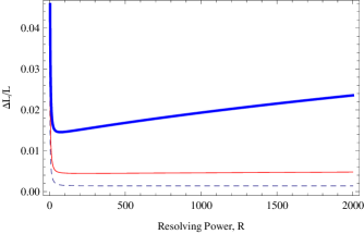
Figure 1: RPE in luminosity from turbulent dissipation for optically thin case at $r=10$AU for the parameters of LLRL 31 as a function of resolving power $R_{ef}$ for $\alpha=0.1(\text{Thick lined Blue}),0.01(\text{thin lined Red}),0.001(\text{Dashed})$. The higher $\alpha$ has the most prominent minimum, which does not correspond to the maximum resolving power but an intermediate value.

4 Implications for Multi-epoch Observations

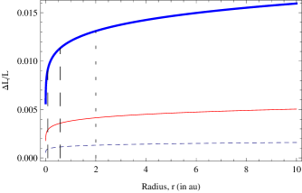
Figure 2: RPE in luminosity from turbulent dissipation vs. radius $r$ for the optically thin case, using $\alpha=0.1(\text{thick lined Blue}),0.01(\text{thin lined Red}),0.001(\text{Dashed})$. From left to right the three vertical dashed lines correspond to three specific radii whose orbit period equals different inter-epoch observation periods for LRLL 31 (Muzerolle et al., 2009): 1 week ($r=0.087$ AU) and 4 months($r=0.58$ AU), and $\sim$ 25 months ($r=2$ AU). For the respective inter-epoch periods, these vertical lines mark the upper radial limit of observational validity of the curves, and above which the expected variability will be sharply reduced. For example, if the inter-epoch interval is 25 months, then the RPE would predict the regime of validity for the curves to be $r<2\AU$. Above $r>2$ AU the prediction would be that $\Delta L_{\nu}/L_{\nu}$ falls near zero because the epochs would sample data from the same statistical ensemble.

A basic application of the RPE described above arises for multi-epoch observations of a single object when the time scale for a snapshot observation is shorter than the eddy time at any radius. Emission from radii at which the time scale between epochs of observation exceeds the eddy turnover time would then be expected to vary stochastically between epochs. In contrast, at radii larger than the that at which the eddy turnover time matches the epoch interval time, successive observations sample the same member of the statistical ensemble and no stochastic variability corresponding to the the local energy-dominating eddies would be expected.

4.1 Lessons from the specific case of LRLL 31

Presently, multi-epoch data are sparse. Programs such as YSOVAR (Stauffer et al., 2010) will eventually produce more data. Nevertheless, to focus the practical application on a on a specific object, we consider IR Spitzer multi epoch observations of the source LRLL 31 in the star-forming region IC 348 (Muzerolle et al., 2009) . For reasons discussed below, this object is most likely not showing its primary variability from stochastic effects we discuss but our analysis to reach this conclusion below illustrates how to use the concepts of the present paper to arrive at that conclusion.

The stellar mass of LRLL 31 is $M=1.8M_{\odot}$ and the estimated accretion rate is $\dot{M}=1.5\times 10^{-8}M_{\odot}{\rm yr}^{-1}({\rm from\ }\text{Pa}\beta)$. For the low spectral resolution mode used to observe this source in the 5-38 micron range (Muzerolle et al., 2009), the Spitzer spectral resolving power is $R\sim 200$. The observation times are minutes, well below the smallest relevant orbit time and consistent with setting $t_{obs}\sim 0$ in (12) and (14) and out assumption throughout the previous sections.

Figure 2 shows Eq. (30) plotted as a function of radius for three different values of $\alpha$ and a value of $R_{ef}=200$ for the optically thin case. The vertical lines show, for three separate choices of the inter-epoch time, the radii above which there would be no variability expected because the inter-epoch time is less than the eddy turnover time above these radii.

Tables 2 and 3 exemplify how use of $R_{ef}=R$, the resolving power for the telescope, compares to the use of $R_{ef}=R_{opt}$, the value that minimizes the luminosity RPE, for different choices of $r$ and $\alpha$. For these tables, the epoch time is taken to exceed the eddy turnover time at all radii. In reality, as emphasized by the vertical lines in Figure 2, there would be negligible expected variability at radii above which the orbit time ($\sim$ eddy turnover time) exceeds a chosen inter-epoch observation interval. For cases in which the telescope resolution (column 6) exceeds the optimal value (column 4) the data can in principle be binned such that the binned data can be compared to the optimal $\alpha$-disc model prediction. The tables highlight two trends in the Tables: (i) the larger the value of $\alpha$ the larger the predicted variability between epochs at a given radius and (ii) the larger the radius for a fixed $\alpha$ the larger the predicted variability.

Muzerolle (2009) argue that the disc of LLRL 31, at $r<10$ AU, is optically thin and substantially cleared out (perhaps via the action of planet) below $10$AU but optically thick for a least some range of larger radii. Thus for this object, the values in the Table 2 would apply for $r<10$AU and the values of table 3 may apply for some range of larger radii above which the disc again becomes optically thin. The value at which the latter occurs requires more detailed modeling.

There is also a transition radius above which viscous dissipation would be dominated by irradiation from the central star (Sicilia-Aguilar et al., 2006; Edgar et al., 2007), namely

$$r_{c}=0.3AU\left(\frac{\dot{M}_{\ast}}{10^{-8}M_{\odot}yr^{-1}}\right)^{\frac{3}{4}}\left(\frac{M_{\ast}}{M_{\odot}}\right)^{\frac{7}{6}}\left(\frac{L_{\ast}}{L_{\odot}}\right)^{-\frac{5}{6}}.$$ (34)

For $r>r_{c}$ the photospheric temperature induced by viscous dissipation falls below that associated from surface dust illumination by the central star. The values of $p$ would then flatten to $p=1/3$ (see Table 1) and irradiation would dominate at all larger radii. Disc emission resulting from stellar irradiation is less influenced by the stochasticity of turbulence than emission via turbulent dissipation. Since the local blackbody emission varies with $T^{3}$, we would expect a much reduced stochastic variability in regions of the disc dominated by emission from reprocessed starlight. This implies that even for epoch intervals longer than the orbit periods at $r>r_{c}$ that the stochastic variability discussed herein would be reduced compared to regions of $r<r_{c}$ It is important to emphasize that the RPEs calculated in Tables 2 and 3 is a stochastic variability corresponding to that of mean field $\alpha$-disc resulting from the disc luminosity contribution by stochastic process such as turbulent viscous dissipation. As applied to the specific object LLRL 31 therefore, these would only amount to a variability in a subdominant contribution to the total emission above $r_{c}$.

An absence of observed stochastic fluctuations for $r>r_{c}$ would support the expectation that the primary emission in those regions is not the result of turbulent dissipation. For $r<r_{c}$ the absence of stochastic variability would be expected only if the inter-epoch time scale is shorter than the characteristic eddy turnover time at the radius dominating the radiation at the particular frequency measured. Note also that the amplitude of the predicted stochastic variability would not depend on the epoch interval as long as the epoch interval is larger than the orbit time at the radius producing the corresponding emission. Other systematic non-axisymmetry or variable accretion rates would add to the variability and could be distinguished form stochastic effects given enough multi-epoch observations

For the specific case of LRLL 31, the largest time scale between epochs is of order 4 months which means that according to Fig. 2, the stochastic variability would be expected only for $r<0.58$ AU. This is well within the dust depleted inner region of this transitional object where the disc is optically thin and where the emission would come from dissipation internal to the disc rather than reprocessed starlight. Thus there would be some stochastic contribution to the measured variability between epochs predicted by the RPE of the mean field models. However, the double-digit percentages of the observed variability reported by Muzerolle et al. (2009) in LRLL 31 are larger than the values predicted in our Tables that arise from stochastic variability alone In addition, the presence of a single pivot wavelength of 8.5 microns (see Fig 1 of Muzerolle et al. (2009)) at which there is no variability in this source and above which the sign of the variability between epochs changes sign from that at low wavelengths strongly suggests the influence of a global geometric feature such as a thick wall or a warp. In short the dominant variability in LRLL 31 object likely comes from systematic rather than stochastic effects.

5 Conclusions

For $\alpha$ models of turbulent accretion discs we have derived a predicted RPE in the luminosity as function of frequency, focusing on the case in which the observational exposure times are small compared ti other dynamical time scales. We have discussed the implications for interpreting multi-epoch spectral observations of spatially unresolved protoplanetary discs.

The RPE depends on the radial scale of averaging and there exists an optimal scale that minimizes the error which also corresponds to an optimal spectral resolution when the correspondence between peak frequency of emission and radius is made. The data can be binned to compare with the theory of minimum RPE only when the spectral resolution of the telescope exceeds the value $R_{opt}$ which minimizes the RPE. An optimal resolution exists because if the spectral resolution is too high then the instrument ends up sampling noise and if the spectral resolution is too low, then the instrument samples overly coarsely binned regions of the disk.

The stochastic variability expected between multi-epoch observations of discs is an implicit prediction of alpha disc theory and can be directly compared to observed variabilities. Complementarily, the nature of the observed variability can be used to constrain whether or not the behavior of the disc is consistent with luminosity produced by stochastic or systematic processes.

The predicted stochastic variability from $\alpha$ discs has several distinct characteristics that would signature its prevalence:

$\bullet$ The stochastic variability is predicted primarily for regions where the luminosity is dominated by internal turbulent dissipation in the disc. For regions dominated by surface dust-reprocessed starlight, the stochastic variability could be expected to be strongly reduced.

$\bullet$. For regions of the discs dominated by from turbulent dissipation, the strength of the stochastic variabilty would increase gradually with decreasing emission frequency (and thus increasing radius) down to a critical frequency below which the associated disc radii have orbital times exceeding the inter-epoch observation time. There the expected variability from the RPE would drop sharply.

$\bullet$ For inner regions of the discs in transitional objects, where emission may be dominated by turbulent dissipation but the discs are optically thin, the stochastic variability would be expected to be lower than that expected from the same radii for optically thick turbulent dissipation dominated discs.

In applying the basic ideas herein to the specific case of LRLL 31, we find that systematic variability NOT stochastic variability dominates. This is indeed consistent with the conclusion of Muzerolle et al. (2009). As more multi-epoch observations of broader samples of discs at different stages in their lifetimes are obtained, the present work may help provide a tool to distinguish stochastic processes in discs from systematic dynamical changes and the time scales on which these occur.

Two overall lessons from this analysis are: (1) the precision of axisymmetric accretion theories can be quantified and deviations the alpha-accretion disc theory and observations at a given epoch cannot rule out the theory if the deviations between epochs exhibit stochastic behavior and fall within the expected RPE of the theory. The theory may be incomplete but because a mean field theory for a turbulent system is intrinsically imprecise, but the imprecision must be quantified so that the user realizes its limitations. (2) Arbitrarily high spectral resolution can lead to misleading comparisons between theory and observation and binning the data may be necessary to compare the data with the theory of minimum RPE.

r(au)	$\alpha$	$R_{\text{opt}}$	${\Delta L_{\nu}\over L_{\nu}}$ (%)	$R_{\text{tel}}$	${\Delta L_{\nu}\over L_{\nu}}$(%)
0.1	0.001	1832	0.08754	200	0.09226
	0.01	579.3	0.2781	200	0.2816
	0.1	183.2	0.8914	200	0.8915
1	0.001	1156	0.1103	200	0.1139
	0.01	365.5	0.3514	200	0.3531
	0.1	115.6	1.135	200	1.144
10	0.001	729.3	0.1392	200	0.1417
	0.01	230.6	0.4449	200	0.4451
	0.1	72.93	1.454	200	1.513
20	0.001	634.9	0.1493	200	0.1515
	0.01	200.8	0.4780	200	0.4780
	0.1	63.49	1.570	200	1.661

Table 2: Optically Thin Case. In column 4, we list the RPE varibilities calculated using $R_{ef}=R_{opt}$ and and in column 6 the values corresponding to the Spitzer telescope low mode $R_{ef}=R_{tel}\sim 200$. The RPEs are computed from Eq. (32) for different $r$ and $\alpha$ and $h/r$ from Eq. (33) using $p=0.6$. The optimal resolution is calculated from Eq. (22) as described below Eq. (33). Note that if $R_{opt}<R_{tel}$ data can be binned to compare with the $\alpha$-disc model of minimal RPE.

r(au)	$\alpha$	$R_{\text{opt}}$	${\Delta L_{\nu}\over L_{\nu}}$(%)	$R_{\text{tel}}$	${\Delta L_{\nu}\over L_{\nu}}$(%)
0.1	0.001	625.8	0.6935	200	0.7111
	0.01	249.2	1.116	200	1.118
	0.1	99.19	1.835	200	1.881
1	0.001	557.8	0.7355	200	0.7510
	0.01	222.1	1.186	200	1.186
	0.1	88.40	1.958	200	2.030
10	0.001	497.1	0.7802	200	0.7935
	0.01	197.9	1.260	200	1.260
	0.1	78.79	2.091	200	2.200
20	0.001	480.2	0.7942	200	0.8069
	0.01	191.2	1.284	200	1.284
	0.1	76.10	2.133	200	2.256

Table 3: same as Table 2 but for optically thick case. The RPEs are computed from Eqs. (25) and (31) for different $r$ and $\alpha$ and for the optically thick version of $h/r$ in Eq. (26) and $p=0.9$.

References

- Balbus and Hawley (2003) Balbus, S. A. and Hawley, J. F.: 2003, in E. Falgarone & T. Passot (ed.), Turbulence and Magnetic Fields in Astrophysics, Vol. 614 of Lecture Notes in Physics, Berlin Springer Verlag, pp 329–348
- Blackman (1998) Blackman, E. G.: 1998, MNRAS 299, L48
- Blackman (2010) Blackman, E. G.: 2010, Astronomische Nachrichten 331, 101
- Edgar et al. (2007) Edgar, R. G., Quillen, A. C., and Park, J.: 2007, MNRAS 381, 1280
- Frank et al. (2002) Frank, J., King, A., and Raine, D. J.: 2002, Accretion Power in Astrophysics: Third Edition, Cambridge University Press
- Hartmann (2009) Hartmann, L.: 2009, Accretion Processes in Star Formation: Second Edition, Cambridge University Press
- Muzerolle et al. (2009) Muzerolle, J., Flaherty, K., Balog, Z., Furlan, E., Smith, P. S., Allen, L., Calvet, N., D’Alessio, P., Megeath, S. T., Muench, A., Rieke, G. H., and Sherry, W. H.: 2009, ApJ 704, L15
- Pringle (1981) Pringle, J. E.: 1981, ARA&A 19, 137
- Shakura and Sunyaev (1973) Shakura, N. I. and Sunyaev, R. A.: 1973, A&A 24, 337
- Sicilia-Aguilar et al. (2006) Sicilia-Aguilar, A., Hartmann, L., Calvet, N., Megeath, S. T., Muzerolle, J., Allen, L., D’Alessio, P., Merín, B., Stauffer, J., Young, E., and Lada, C.: 2006, ApJ 638, 897
- Spruit (2010) Spruit, H. C.: 2010, ArXiv e-prints
- Stauffer et al. (2010) Stauffer, J. R., Megeath, T., Rebull, L., Morales, M., Plavchan, P., Gutermuth, R., Inseok, S., Carey, S., Covey, K., and YSOVAR/Orion team: 2010, in Bulletin of the American Astronomical Society, Vol. 41 of Bulletin of the American Astronomical Society, pp 350–+
Acknowledgments
The authors acknowledge support from NSF grants AST-0406799, AST-0098442, AST-0406823, and NASA grants ATP04-0000-0016 and NNG04GM12G (issued through the Origins of Solar Systems Program). FN acknowledges a Horton Fellowship from the Laboratory for Laser Energetics at U. Rochester.