Solution of three-dimensional Faddeev equations: ultracold Helium trimer calculations with a public quantum three-body code
Abstract
We present an illustration of using a quantum three-body code being prepared for public release. The code is based on iterative solving of the three-dimensional Faddeev equations. The code is easy to use and allows users to perform highly-accurate calculations of quantum three-body systems. The previously known results for He3 ground state are well reproduced by the code.
Keywords:
three-body atomic systems, Faddeev equations, Helium trimer, ultracold collisions:
21.45.-v, 31.15.ac, 34.10.+x, 36.90.+f, 02.70.Jn1 Introduction
The quantum few-body problem is important for investigating physical processes at practically all possible length and energy scales. For instance, three-body models can be employed for describing nuclear reactions Friar ; dd ; alphaBe ; Lambda , electron- and positron-atom collisions Hu ; Rescigno , and chemical reactions HNe2 . The developments of the last decade demonstrated the importance of three-body processes for understanding the dynamics of ultra-cold gases EsryGreen . An ability to solve a few-body problem directly would also be beneficial to theorists for testing, for instance, effective-field theories Braaten ; Phillips .
The three-body problem, however, has sufficient intrinsic complexity that it often inhibits or prevents non-experts in few-body calculations from considering realistic three-body models and from employing physically correct representations BadHelium . Accordingly, a standard, easily operable and rigorously constructed tool for three-body calculations will be beneficial for a broad physical community. Such a tool should be tested independently to ensure its usability and applicability. This work is a result of a collaboration between the authors of this tool, developed at the University of Kentucky, and a research group in JINR performing independent tests.
In the following sections we describe the equations being solved and report the results of the tests we have performed.
2 Formalism
The three-body code being tested is based on solving Faddeev equations in configuration space. The complete and mathematically rigorous theory of Faddeev equations can be found in books on the topic MerkFadd ; Integral ; SchmidtZigelman . Here we only sketch out the gross features important for understanding and using the code.
We start by describing the physical model from the three-body Hamiltonian
| (1) |
where stands for the kinetic energy of the three particles, is the interaction potential acting in the pair , and is a short-range three-body interaction. (In the following description the latter will be omitted only for simplicity. Taking into account the three-body interactions, however, does not produce any practical or principal difficulties.) The configuration space of the three particles is described in terms of 3 sets of Jacobi coordinates
| (2) |
The set of coordinates describes a partitioning of the three particles into a pair and a separate particle . Faddeev decomposition represents the wave function in terms of a sum over all possible partitioning of the three-body system
| (3) |
Faddeev components, , satisfy the following set of equations MerkFadd
| (4) |
where and are mass-weighted Jacobi coordinates, is the interaction potential in the -th pair and is the total energy of the system. It is not difficult to prove that the exact wave function of the three body system can be uniquely constructed from the Faddeev components by means of Eq. (3).
The equations in six-dimensional space can hardly be solved directly, and some partial analysis is necessary. We consider the states with zero total angular momentum. The angular degrees of freedom corresponding to collective rotation of the three-body system can be separated Kvits and the kinetic energy operator reduces to
| (5) |
where , and are so called intrinsic coordinates
| (6) |
In the case of identical bosons Faddeev components take identical functional form, which makes it possible to reduce the system of three equations (4) to one equation
| (7) |
where
and , , and are
| (8) |
Assuming that in each two-body subsystem only one bound state exists, we can write the asymptotic boundary conditions for the Faddeev component as follows
| (9) |
where stands for the wave function of the two-body subsystem bound state, , , is the two-body bound state energy, and the energy of the three-body system. For three-body bound states the first term corresponds to virtual decay into a particle and a two-body bound system, while the second term corresponds to a virtual decay with an amplitude into three single particles. The term corresponding to the latter configuration can generally be neglected for the states below the three-body threshold. Therefore, at sufficiently large distances and , the asymptotic boundary conditions for the Faddeev component are
| (10) |
For bound state calculations Dirichlet or Neumann boundary conditions can also be employed.
The important property of the Faddeev components which makes them suitable for numerical solution is their simple asymptotic form. For instance, each of the Faddeev components holds only bound states of the corresponding two-body subsystem. In this respect the coordinate is the internal coordinate of the corresponding two-body cluster and the coordinate plays the role of a reaction coordinate for all the states below the 3-body (break-up) threshold. This simple physical meaning of the coordinates suggest a natural requirement for discretizing the corresponding degrees of freedom: the discrete analogs of the coordinate should reproduce the spectrum of the -th cluster correctly, and discrete analogs of the coordinate must describe the scattering states reasonably well. These necessary requirements are easy to check prior to performing actual calculations, and they also provide a solid ground for a reasonable degree of automation for choosing the parameters of the numerical scheme. Another advantage of the Faddeev equations is the asymptotic decoupling of the components. The right-hand side of the equation (4) is, roughly speaking, exponentially small if the third particle is at larger distance than the typical size of the two-body bound state. This means that at longer distances the Faddeev components rapidly decouple, and calculations can be performed in the regions as small as the size of the largest two-body subsystem bound state.
The advantages of the Faddeev approach can be exploited even further when dealing with short-range interactions; i.e. assuming that the potentials are zero (or negligible) outside the region . To clarify this, consider the component in the asymptotic region , , where it satisfies a Schrödinger equation with the corresponding channel Hamiltonian
where is the free three-body Hamiltonian. This property of suggests that, rather than calculate directly, we instead calculate (Eq. 11), which is better localized in configuration space
| (11) |
These are non-zero only for small and small . Accordingly, they are localized to a region that can be much smaller than the typical size of a two-body bound state. This feature leads to substantial computational savings myCPL2 . The satisfy the following integral equations
| (12) |
where are the resolvents of the corresponding channel Hamiltonians. Since , the are more suitable for numerical approximation than the original Faddeev components. Furthermore, if the equation is being solved using an iterative technique, then no explicit representation for the integral operators is required. In this case we only need to calculate the action of the integral operator on the , which can be done with high computational efficiency by numerically solving the corresponding differential equation with appropriate boundary conditions. We call this computational scheme a Localized Component Method (LCM).
3 Computer code
In order to construct a discrete analogue of the system of equations (12) we employ quintic Hermite splines together with the orthogonal collocations method deBoorSwartz . A detailed description of the procedure is given in RoudnevYak . This high-order method guarantees fast convergence with respect to the number of grid points, sparse matrix structure for the discrete analog of the equation (4), and fast calculation of matrix elements that makes it possible to avoid storing big matrices in computer memory.
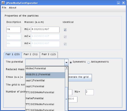
The code is written in Java and consists of two parts. The first part is a configurator that simplifies composing the necessary configuration files. The configurator allows the user to set masses of the interacting atoms, to specify identical particles in the system, to choose a potential model, to set the cutoff distances and and to set the number of grid points to be employed in the calculation. It also generates a mesh with -optimal point distribution which ensures the best possible approximation of the three-body wave function in the asymptotic region. In Fig. 1 we show an example of the configurator screenshot.
The second part is the three-body computational kernel based on the LCM approach. The kernel is currently capable of three-body calculations below the three-body threshold with a limitation of no more than one two-body bound state contributing to each asymptotic channel. This includes bound states, elastic scattering and chemical reactions below the first vibrational excitation threshold. Typical computational time can take from minutes to hours, depending on the physical system and the size of the grid.
4 Results
We apply the code to the calculation of binding energies of the Helium trimer 4He3 three-atomic system, to verify that we can reproduce the known calculated properties of helium trimer ground and excited states. This system is very particular about the approach being used, as the trimer binding energy is extremely small and a large volume of the configuration space should be treated, but the interaction features very strong repulsion at short distances, which requires very precise numerical methods to be used.
Experimentally, helium dimers have been observed for the first time in 1993 by the Minnesota group DimerExp , and in 1994 by Schöllkopf and Toennies Science . Later on, Grisenti et al. exp measured a bond length of Å for 4He2, which indicates that this dimer is the largest known diatomic molecular ground state. Based on this measurement they estimated a scattering length of Å and a dimer energy of mK exp . In the latter investigation HeEfimovExp the trimer pair distance is found to be nm in agreement with theoretical predictions for the ground state.
Many theoretical calculations of these systems were performed for various interatomic potentials Aziz91 ; TTY . Variational Orlandini ; Bressanini , hyperspherical EsryGreen ; BlumeGreene ; Barletta09 and Faddeev techniques myCPL2 ; RoudnevYak ; kea ; SalciLevin ; Lazauskas ; MSSK have been employed in this context. It was found that the Helium trimer has two bound states of total angular momentum zero: a ground state of about mK and an excited state of Efimov-type of about mK. Experimentally this Efimov-typeEfimov excited state has not yet been observed (see, e.g., Review2009 and refs. therein). It should be mentioned, however, that the year 2006 is noticeable due the first convincing experimental evidence for the Efimov effect in an ultracold gas of Caesium atoms Nature2006 ; Nature_th .
In present calculations we employed the code based on the Faddeev differential equations (5) with boundary conditions (10). As He-He interaction we used the semi-empirical LM2M2 potential Aziz91 . We use for the mass of the 4He atom and K Å2, unlike many three-body calculations, see, e.g., Review2009 , where a rounded value of the coefficient has been used.
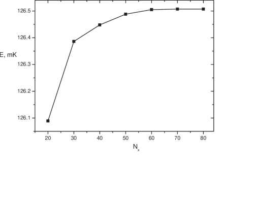
Investigation of the bound state energy convergence with respect to the number of grid points demonstrates that even a moderate number of points in variables and is sufficient to get up to six accurate figures for the energy of the ground state (Fig. 2).
| Potential model | (mK) | (Å) | (Å) | (Å) |
| LM2M2 Aziz91 | 100.23 | 52.001 | 70.926 | |
| Exp. exp | - |
The 4He dimer binding energies, 4He–4He scattering lengths and mean values of the radius and obtained with the LM2M2 potential Aziz91 are shown in Table 1 in comparison with experimental data exp . All the values agree with an experimental estimation of Ref.exp within quoted errors. The scattering length of the system is bigger than the range of the potential by an order of magnitude. All these features characterize the Helium dimer as the weakest, as well as the biggest, diatomic molecule found so far. Due to the fact that the energy of the dimer is so small, one should expect that the trimer indeed possesses the theoretically predicted state of the Efimov type (see, Efimov ; Review2009 ).
In Table 2 the results of trimer binding energies calculations obtained with LM2M2 potential are summarized. The binding energies of the 4He trimer ground () and exited () states are presented. These results demonstrate good agreement between different methods and show that the code competes well even against variational methods. It should be mentioned that the energy estimates obtained with the code are non-variational, and further variational improvements of the results are possible.
| present | kea | RoudnevYak | SalciLevin | Lazauskas | MSSK | BlumeGreene | Barletta09 | Orlandini | |
|---|---|---|---|---|---|---|---|---|---|
| (mK) | 126.41 | 126.39 | 125.9 | 111 | 126.15 | ||||
| (mK) | 2.271 | 2.268 | 2.282 | 2.274 |
We are planning to continue testing the code within current applicability limits, including scattering calculations, systems of distinguishable particles and modeling clusters of other rare gas atoms.
References
- (1) J. L. Friar, B. F. Gibson, G. Berthold, W. Glöckle, Th. Cornelius, H. Witala, J. Haidenbauer, Y. Koike, G. L. Payne, J. A. Tjon, and W. M. Kloet, Phys. Rev. C 42, 1838–1840 (1990).
- (2) S. L. Yakovlev, I. N. Filikhin, Phys. Atom. Nucl. 60, 1794–1802 (1997).
- (3) E. Garrido, D. V. Fedorov and A. S. Jensen, Phys. Rev. C 59, 1272–1289 (1999).
- (4) I. Filikhin, A. Gal, V. M. Suslov, Nucl. Phys. A 743, 194–207 (2004).
- (5) C.-Y. Hu, S. L. Yakovlev and Z. Papp, Nucl. Instr. and Methods in Physics Research B 247, 25–30 (2006).
- (6) C. W. McCurdy, M. Baertschy, T. N. Rescigno, J. Phys. B 37, R137–R187 (2004).
- (7) G. A. Parker, R. B. Walker, B. K. Kendrick, and R. T. Pack, J. Chem. Phys. 117, 6083–6085 (2002).
- (8) B. D. Esry, C. H. Greene, Y. Zhou and C. D. Lin, J. Phys. B 29, L51–L57 (1996).
- (9) E. Braaten and H.-W. Hammer, Phys. Rev. Lett. 87, 160407 (2001); P. F. Bedaque, E. Braaten, and H.-W. Hammer, Phys. Rev. Lett. 85, 908–911 (2000).
- (10) I. R. Afnan and D. R. Phillips, Phys. Rev. C 69, 034010 (2004).
- (11) T. Gonzalez-Lezana, J. Rubayo-Soneira, S. Miret-Artes, F. A. Gianturco, G. Delgado-Barrio, and P. Villarreal, Phys. Rev. Lett. 82, 1648–1651 (1999).
- (12) L. D. Faddeev and S. P. Merkuriev, Quantum Scattering Theory for several particle systems. Doderecht: Kluwer Academic Publishers, 1993.
- (13) V. B. Belyaev, Lectures on the Theory of Few-Body Systems, Springer Verlag, 1990.
- (14) E. Schmidt and H. Ziegelmann, The Quantum Mechanical Three Body Problem, Pergamon, 1974.
- (15) V. V. Kostrykin, A. A. Kvitsinsky, and S. P. Merkuriev, Few-Body Systems, 6, 97–113 (1989).
- (16) V. A. Roudnev, Chem. Phys. Lett. 367, 95–101 (2003).
- (17) C. de Boor and B. Swartz, SIAM J. Numer. Anal. 10, 582–606 (1973).
- (18) V. A. Roudnev, S. L. Yakovlev, S. A. Sofianos, Few-Body Systems, 37, 179–196 (2005).
- (19) F. Luo, G. C. McBane, G. Kim, C. F. Giese, W. R. Gentry, J. Chem. Phys. 98, 3564–3567 (1993).
- (20) W. Schöllkopf and J. P. Toennies, Science, 266, 1345–1348 (1994).
- (21) R. Grisenti, W. Schöllkopf, J. P. Toennies, G. C. Hegerfeld, T. Köhler, M. Stoll, Phys. Rev. Lett. 85, 2284–2287 (2000).
- (22) R. Brühl, A. Kalinin, O. Kornilov, J. P. Toennies, G. C. Hegerfeld, M. Stoll, Phys. Rev. Lett. 95, 06002 (2005).
- (23) R. A. Aziz and M. J. Slaman, J. Chem. Phys. 94, 8047–8053 (1991).
- (24) K. T. Tang, J. P. Toennies, and C. L. Yiu, Phys. Rev. Lett. 74, 1546–1549 (1995).
- (25) D. Bressanini, M. Zavaglia, M. Mella, G. Morosi, J. Chem. Phys. 112, 717–722 (2000).
- (26) S. Orlandini, I. Baccarelli, F. A.Gianturco, Comp. Phys. Comm. 180, 384–391 (2009).
- (27) D. Blume, C. H. Greene, J. Chem. Phys. 112, 8053–8067 (2000).
- (28) P. Barletta and A. Kievsky, Few-Body Systems, 45, 123–125 (2009).
- (29) E. A. Kolganova, Physics of Particles and Nuclei, 41, 1108–1110 (2010).
- (30) M. Salci, E. Yarevsky, S. B. Levin, N. Elander, Int. J. Quant. Chem. 107, 464–468 (2007).
- (31) R. Lazauskas, J. Carbonell, Phys. Rev. A 73, 062717(11) (2006).
- (32) A. K. Motovilov, W. Sandhas, S. A. Sofianos, E. A. Kolganova, Eur. Phys. J. D13, 33–41 (2001).
- (33) V. Efimov, Nucl. Phys. A 210, 157–188 (1973); Phys. Lett. B 33 563–564 (1970).
- (34) E. A. Kolganova, A. K. Motovilov, W. Sandhas, Physics of Particles and Nuclei, 40, 206–235 (2009).
- (35) T. Kraemer, M. Mark, P. Waldburger, J. G. Danzl, C. Chin, B. Engeser, A. D. Lange, K. Pilch, A. Jaakkola, H.-C. Nagerl and R. Grimm, Nature, 440, 315–318 (2006).
- (36) B. D. Esry and C. H. Greene, Nature, 440, 289–290 (2006).