Gluon polarisation from high transverse momentum hadron pairs production @ COMPASS

Abstract

A new preliminary result of a gluon polarisation $\Delta G/G$ obtained selecting high transverse momentum hadron pairs in DIS events with $Q^{2}>1\ (\mbox{GeV/}c)^{2}$ is presented. Data has been collected by COMPASS at CERN during the 2002-2004 years. In the extraction of $\Delta G/G$ contributions coming from the leading order $\gamma q$ and QCD processes are taken into account. A new weighting method based on a neural network approach is used. Also a preliminary result of $\Delta G/G$ for events with $Q^{2}<1\ (\mbox{GeV/}c)^{2}$ is presented.

1 Introduction

Deep inelastic scattering (DIS) of leptons on nucleons is an important tool to reveal the inner structure of the nucleon. The DIS experiment at SLAC in the 60’s showed the scaling predicted by J. Bjorken, in the limit $Q^{2}\rightarrow\infty$; this discovery was celebrated in 1990 by the Nobel Prize in Physics awaded to J.I. Friedman, H.W. Kendal and R.E. Taylor. The observation of this scaling was the first evidence of point-like constituents inside the nucleon.

DIS of polarised leptons on polarised nucleons is a tool to study the spin structure of the nucleon. The first experiments using polarised ep scattering were perfomed by the E80 Alguard:1976bm and E130 Baum:1983ha Collaborations at SLAC, measuring the spin-dependent asymmetries with a significant value consistent with the Ellis-Jaffe sum rule ellis-jaffe . Surprisingly on 1987 the EMC experiment at CERN, with an extended kinematic range down to $0.01<x$, announced that, contradicting previous results and predictions, the measured quark contribution to nucleon spin is small ($0.12\pm 0.17$) emc and its result has been confirmed by other experiments Abe:1997cx ; Abe:1998wq ; Anthony:1996mw ; Anthony:1999py ; Adams:1997tq ; Airapetian:1998wi . In 2007, COMPASS collaboration measured this contribution with a higher precision comp.del_sigma , using a NLO QCD fit with all world data available including 43 points measured by COMPASS, confirms that approximately 1/3 of the spin is carried by the quarks.

Since the quark contribution does not account fully for the nucleon spin some contributions need to be found to solve this “spin crisis”. As nucleons are also made of gluons together with quarks, the most natural would be to include the contributions from the gluons and from orbital angular momentum.

Thus the nucleon spin can be written as:

$$\frac{1}{2}=\frac{1}{2}\Delta\Sigma+\Delta G+L$$ (1)

$\Delta\Sigma$ and $\Delta G$ are, respectively, the quark helicity and gluon contributions to the nucleon spin and $L$ is the contribution to the nucleon spin coming from orbital angular momentum from the partons (quarks and gluons).

The aim of this study is to estimate the gluon polarisation using the high transverse momentum (high $p_{T}$) hadron pairs. The analysis is performed in two complementary kinematic regions: $Q^{2}<1\ (\mbox{GeV}/c)^{2}$ (low $Q^{2}$ region) and $Q^{2}>1\ (\mbox{GeV}/c)^{2}$ (high $Q^{2}$ region). The present work is mainly focused on the analysis for high $Q^{2}$. However, the analysis at low $Q^{2}$ region is summarised in section 7.

2 Analysis Formalism

Spin-dependent effects can be measured experimentally using the helicity asymmetry

$$A_{\rm LL}=\frac{\Delta\sigma}{2\sigma}=\frac{\sigma^{\uparrow\Downarrow}-\sigma^{\uparrow\Uparrow}}{\sigma^{\uparrow\Downarrow}+\sigma^{\uparrow\Uparrow}}$$ (2)

defined as the ratio of polarised ($\Delta\sigma$) and unpolarised ($\sigma$) cross sections. $\uparrow\Uparrow$ and $\uparrow\Downarrow$ refer to the parallel and anti-parallel configuration of the beam lepton spin ($\uparrow$) with respect to the target nucleon spin ($\Uparrow$ or $\Downarrow$).

According to the factorisation theorem, the (polarised) cross sections can be written as

$$\sigma=\sum_{i}e^{2}_{i}q_{i}\otimes\hat{\sigma}\otimes D$$ (3)

$$\Delta\sigma=\sum_{i}e^{2}_{i}\Delta q_{i}\otimes\Delta\hat{\sigma}\otimes D$$ (4)

i.e. the convolution of the parton distribution functions, ($\Delta$)$q_{i}$, the hard scattering partonic cross section, ($\Delta$)$\hat{\sigma}$, and the fragmentation function $D$.

The gluon polarisation is measured directly via the Photon-Gluon Fusion process (PGF); which allows to probe the gluon inside the nucleon. Two other processes compete with the PGF process in the leading order QCD approximation, namely the virtual photo-absorption leading order (LO) process and the gluon radiation (QCD Compton) process. In Fig. 1 all contributing processes are depicted.

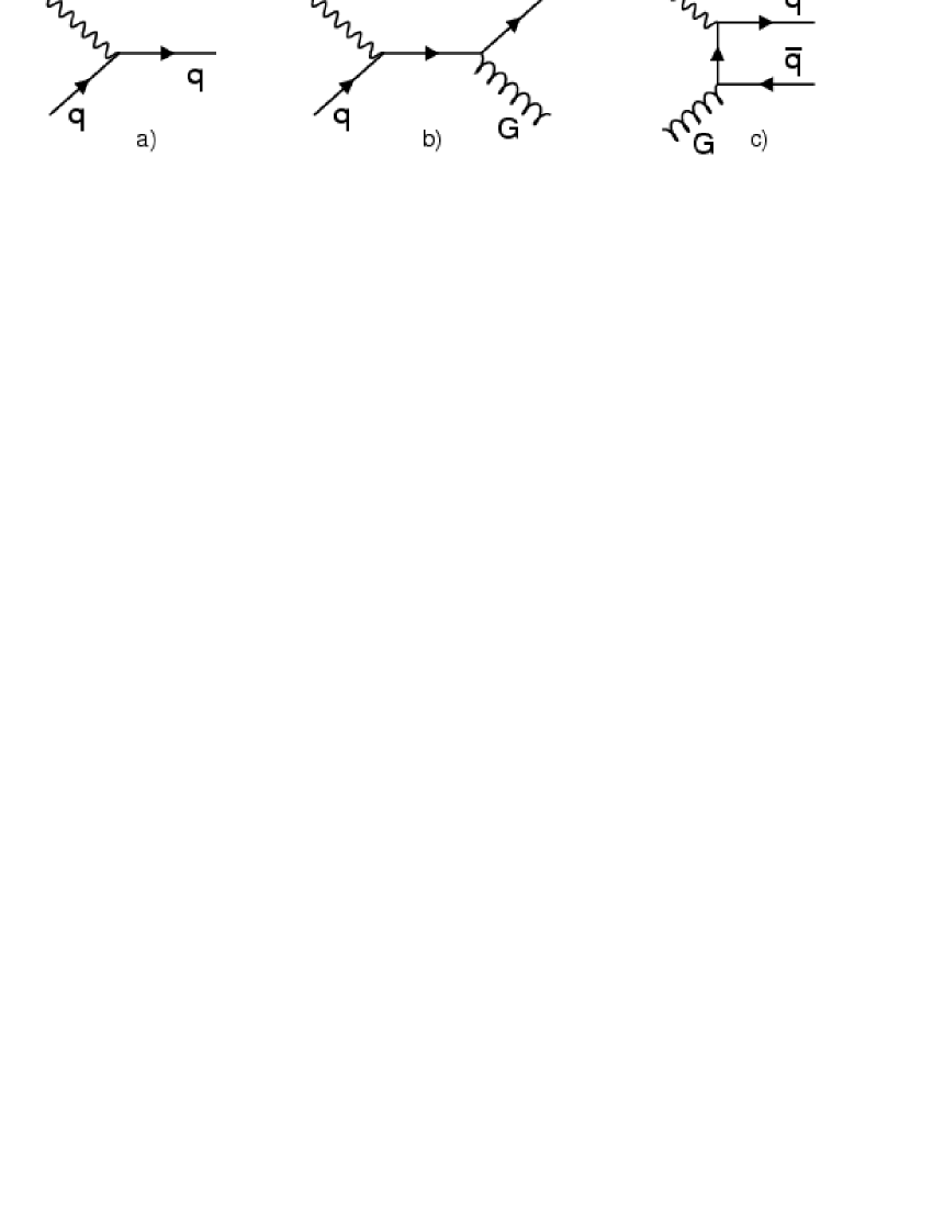
Figure 1: The contributing processes: a) DIS LO, b) QCD Compton and c) Photon-Gluon Fusion.

The helicity asymmetry for the high $p_{T}$ hadron pairs in high $Q^{2}$ regime can be written as:

$$A_{\rm LL}^{2h}(x_{Bj})=R_{\rm PGF}\,a_{\rm LL}^{\rm PGF}\frac{\Delta G}{G}(x_{G})+R_{\rm LO}\,D\,A_{1}^{\rm LO}(x_{Bj})+R_{\rm QCDC}\,a_{\rm LL}^{\rm QCDC}A_{1}^{\rm LO}(x_{C})$$ (5)

The $R_{i}$ (the index $i$ refers to the different processes) are the fractions of each process. $a_{\rm LL}^{i}$ represents the partonic cross section asymmetries, $\Delta\hat{\sigma}^{i}/\hat{\sigma}^{i}$, (also known as analysing power). $D$ is the depolarisation factor. The virtual photon asymmetry $A_{1}^{\rm LO}$ is defined as

$$A_{1}^{\rm LO}\equiv\frac{\sum_{i}e_{i}^{2}\Delta q_{i}}{\sum_{i}e_{i}^{2}q_{i}}.$$ (6)

To extract $\Delta G/G$ from eq. (5) the contribution from the physical background processes LO and QCD Compton need to be estimated. This is done using MC simulation to calculate $R_{i}$ fractions and $a_{\rm LL}^{i}$. The virtual photon asymmetry $A_{1}^{\rm LO}$ was estimated using a parametrisation based on inclusive the $A_{1}$ asymmetry data compassrho .

For the inclusive asymmetry $A_{\rm LL}^{incl}$ a similar decomposition as eq. (5) can be applied:

$$A_{\rm LL}^{incl}(x_{Bj})=R_{\rm PGF}^{incl}a_{\rm LL}^{incl,{\rm PGF}}\frac{\Delta G}{G}(x_{G})+R_{\rm LO}^{incl}DA_{1}^{\rm LO}(x_{Bj})+R_{\rm QCDC}^{incl}a_{\rm LL}^{incl,{\rm QCDC}}A_{1}^{\rm LO}(x_{C}).$$ (7)

Note that $y$, $D$, $x_{Bj}$, $x_{G}$ and $x_{C}$ in the inclusive and high $p_{T}$ sample can be different. The extraction of $\Delta G/G$ requires a new definition of the averaged $x_{G}$ at which the measurement is performed:

$$x_{G}^{av}=\frac{\alpha_{1}x_{G}-\alpha_{2}x_{G}^{\prime}}{\beta}$$ (8)

where:

$$\alpha_{1} = a_{\rm LL}^{\rm PGF}R_{\rm PGF}-a_{\rm LL}^{incl,{\rm PGF}}R_{\rm LO}\frac{R_{\rm PGF}^{incl}}{R_{\rm LO}^{incl}}$$ (9)

$$\alpha_{2} = a_{\rm LL}^{incl,{\rm PGF}}R_{\rm QCDC}\frac{R_{\rm PGF}^{incl}}{R_{\rm LO}^{incl}}\frac{a_{\rm LL}^{\rm QCDC}}{D}$$ (10)

$$\beta = \alpha_{1}-\alpha_{2}.$$ (11)

The definition of $x_{G}^{av}$ relies on the assumption of linear dependence of $\Delta G/G$ on $x_{G}$. This assumption is well justified by the narrow $x_{G}$ bin used.

Using eq. (5 and 7) and neglecting small terms the following expression is obtained:

$$\frac{\Delta G}{G}(x_{G}^{av}) = \frac{A_{\rm LL}^{2h}(x_{Bj})+A^{corr}}{\beta}$$

$$A^{corr} = -A_{1}(x_{Bj})D\frac{R_{\rm LO}}{R_{\rm LO}^{incl}}-A_{1}(x_{C})\beta_{1}+A_{1}(x_{C}^{\prime})\beta_{2}$$ (12)

and

$$\beta_{1} = \frac{1}{R_{\rm LO}^{incl}}\bigg{[}a_{\rm LL}^{\rm QCDC}R_{\rm QCDC}-a_{\rm LL}^{incl,{\rm QCDC}}R_{\rm QCDC}^{incl}\frac{R_{\rm LO}}{R_{\rm LO}^{incl}}\bigg{]}$$

$$\beta_{2} = a_{\rm LL}^{incl,{\rm QCDC}}\frac{R_{\rm QCDC}^{incl}}{R_{\rm LO}^{incl}}\frac{R_{\rm QCDC}}{R_{\rm LO}^{incl}}\frac{a_{\rm LL}^{\rm QCDC}}{D}$$ (13)

The term $A^{corr}$ comprises the correction due to the other two processes; namely the LO and the QCD Compton processes. $\beta_{1}$, $\beta_{1}$, $\beta_{1}$, $x_{C}$ and $x_{G}^{av}$ are estimated using high $p_{T}$ and inclusive MC samples. The gluon polarisation $\Delta G/G$ is extracted using a weight evaluated in a event-by-event analysis describe in section 6.

3 COMPASS Experiment

COMPASS is a deep inelastic scattering experiment located at the Super Proton Synchrotron (SPS) accelerator at CERN. It is dedicated to the study of the spin structure of the nucleon and to hadron spectroscopy. The experimental setup consists in three main components: a polarised muon beam, a polarised target and a two-stage spectrometer.

A $400\ \mbox{GeV/}c$ proton beam extracted from the SPS collides on a beryllium target producing mainly $\pi$ and $K$ mesons. Which are transported through a 600 m long decay channel. Due to the parity violation in weak decays of the parent hadrons ($\pi,\ K\rightarrow\mu\ \nu_{\mu}$) the newly produced muons are naturally polarised at the energy of 160 GeV.

The polarised target is composed by two cylindrical target cells polarised in opposite directions, filled with deuterated lithium (⁶LiD) solid state material. Each cell is 60 cm long and has a radius of 3 cm. They are disposed longitudinally one after the other with a separation of 10 cm and embedded in a superconducting solenoid magnet that provides a very homogeneous field of 2.5 Tesla. The target cells are kept under a temperature below 60 mK. This solenoid magnet was used in the SMC experiment and has a geometric acceptance of $\approx\pm 70$ mrad. In Fig. 2 a drawing of the polarised target is shown.

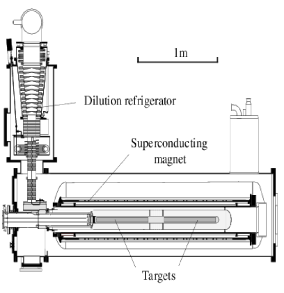
Figure 2: Schematic drawing of the polarised target.

The polarisation method is based on the dynamic nuclear polarisation (DNP) technique Abragam:89a ; the paramagnetic centers, the electrons, of the target cells under the high and homogeneous solenoid magnetic field and at a very low temperature are polarised to high degree. A microwave field is applied to the target material to transfer the polarisation from the paramagnetic centers to the nucleons. Since the desired situation is to have two cells oppositely polarised two independently microwave systems are required. Thus depending on the microwave frequency the nucleon spins of the cells can be polarised parallel or anti-parallel with respect to the beam polarisation. A dipole magnet with a field of 0.5 T perpendicular to the solenoid magnetic field performs the spins rotation of the target cells with respect to beam direction. This field rotation of $180^{\rm o}$ is done in a regular basis to minimise systematics errors due to geometrical acceptance of the solenoid.

The COMPASS spectrometer covers a large kinematic region ($10^{-4}~{}(\mbox{GeV}/c)^{2}<Q^{2}<60\ (\mbox{GeV}/c)^{2}$, $10^{-5}<x_{Bj}<0.5$). Each stage spectrometer is composed by a magnet, tracking chambers and trigger devices. The first spectrometer is disposed downstream after the polarised target, it covers an acceptance of $\pm 180$ mrad and has a bending magnet power of 1 Tm. Therefore this spectrometer is mainly devoted to low momentum particles, it is also known as large angle spectrometer (LAS). The next spectrometer is the small angle spectrometer (SAS) and devoted to high momentum particles, it covers an acceptance of $\pm 30$ mrad, with a bending power of 4.4 Tm. The tracking system is distributed in both stage spectrometers and it can be divided in three main zones: very small area trackers (VSAT) –the set of tracking planes between the solenoid magnet and the LAS magnet– , the small area trackers (SAT) –the set of tracking planes between the LAS and SAS magnets– and large area trackers (LAT) –the set of planes after the SAS magnet–. In Fig. 3 all regions and components of the COMPASS spectrometer are illustrated.

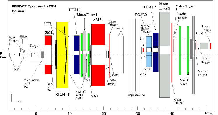
Figure 3: Compass 2004 muon setup top view.

For a more complete description of the experimental apparatus the reader is addressed to compass .

4 Data Selection

The data sample used in this analysis includes data from 2002, 2003 and 2004 years. The selected events have a primary vertex containing an incoming beam muon, a scattered outgoing muon and at least two outgoing hadrons with high transverse momentum.

The following kinematic cuts are applied: $Q^{2}>1\ (\mbox{GeV}/c)^{2}$. A cut applied is on the fraction of energy taken by the virtual photon, $y$: $0.1<y<0.9$; events with $y<0.1$ are rejected because their depolarisation factor is rather low, while events with $y>0.9$ are rejected because they are strongly affected by radiative effects, which are difficult to evaluate.

The incoming muon, $\mu$, is required to cross both target cells, to ensure the same flux. Two particles with highest $p_{T}$ associated with the primary vertex besides the $\mu$ and $\mu^{\prime}$ are considered as hadron candidates. They must fulfil the following requirements:

• The hadron candidates are not muons. There is indeed a small probability for a pile-up muon to be included in the primary vertex and therefore being considered as a hadron candidate. When the energy measurement by the calorimeters is available, the hadron candidate is rejected if $E_{cal}/p<0.3$, where $E_{cal}$ is the total energy measured by the hadronic calorimeters associated to the track of momentum $p$.

• The quality of the track reconstruction is good.

• Hadrons do not go through the solenoid. The hadron tracks are extrapolated to the entrance of the solenoid and then the distance between the track and the z axis should be less than the radius of the solenoid aperture.

The following cuts are applied to the leading (highest transverse momentum) and sub-leading hadrons:

• Both hadrons must have a transverse momentum above $0.7\ \mbox{GeV/c}$. This requirement constitutes the high $p_{T}$ cut.

• $x_{F}>0$, $z>0$ and $z_{1}+z_{2}<0.95$. This last cut is meant to reject events from exclusive production.

• Invariant mass of the two high $p_{T}$ hadrons must be greater than $1.5\ (\mbox{GeV/c})^{2}$. This cut is intended to remove the virtual photon events which fluctuate to a vector meson such as a $\rho$, that afterwards decay into two hadrons.

The number of events and the percentage that survives each cut are displayed in Table 1. In this table, the event candidates are events that pass all kinematic and high $p_{T}$ cuts. PID hadrons refer to event which pass the first cut of hadrons candidates.

	number of events that survive each cut
Cuts	2002	2003	2004	All years	%
Event candidate	89111	309893	524862	923866	100.0
Invariant mass	59711	208055	350989	618755	67.0
PID hadrons	52363	180965	301698	535026	57.9
$x_{F}>0$, $z>0$	51325	176426	294970	522721	56.6
$x_{Bj}>0$, $z_{1}+z_{2}<0.95$	49962	172431	288732	511125	55.3
Hadron quality	49585	170943	286685	507213	54.9

Table 1: Table summarising cuts.

The distributions of the kinematic variables $Q^{2}$, $y$, $x_{Bj}$ are shown in Fig. 4. The distributions of $p$, $p_{T}$, $\sum p_{T}^{2}$ and $z$ variables are presented in Figs. 5 and 6, for the leading and sub-leading hadrons.

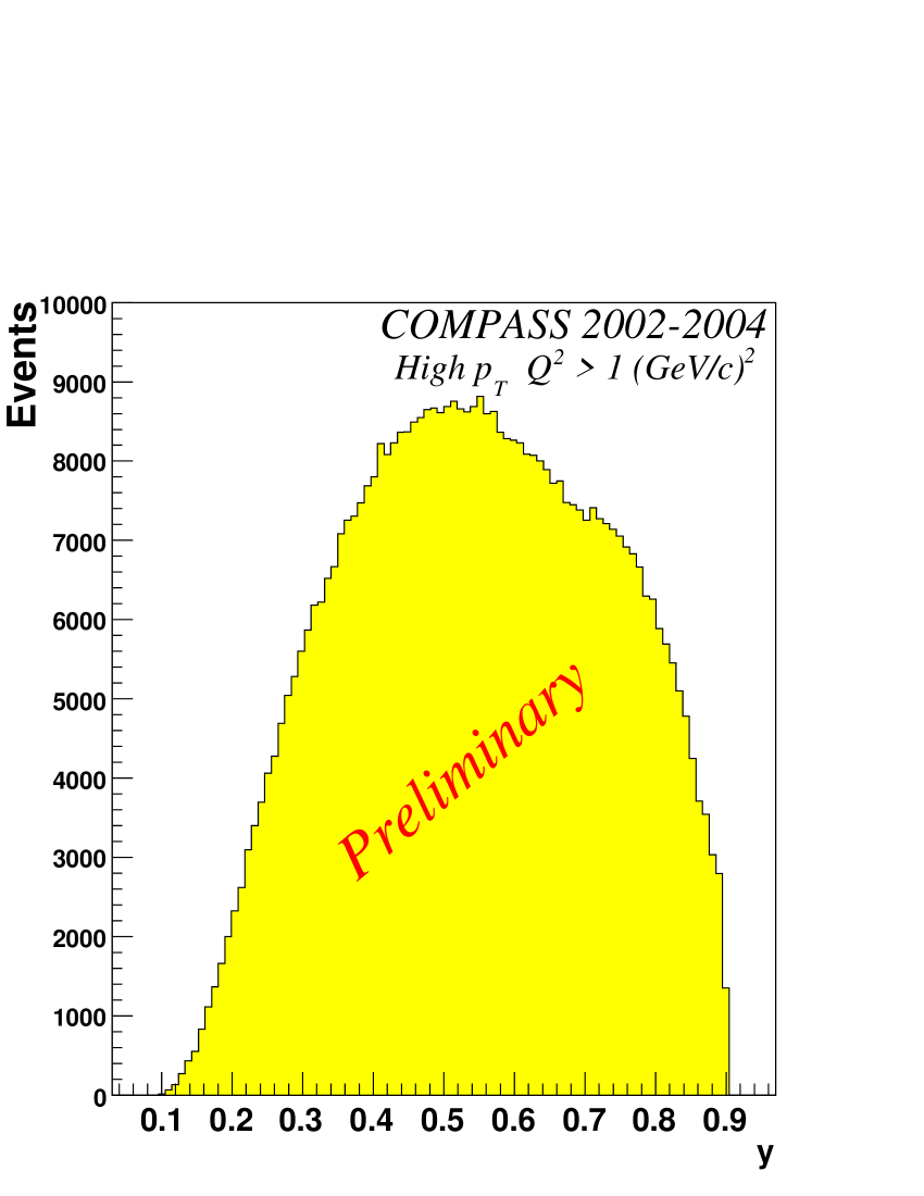
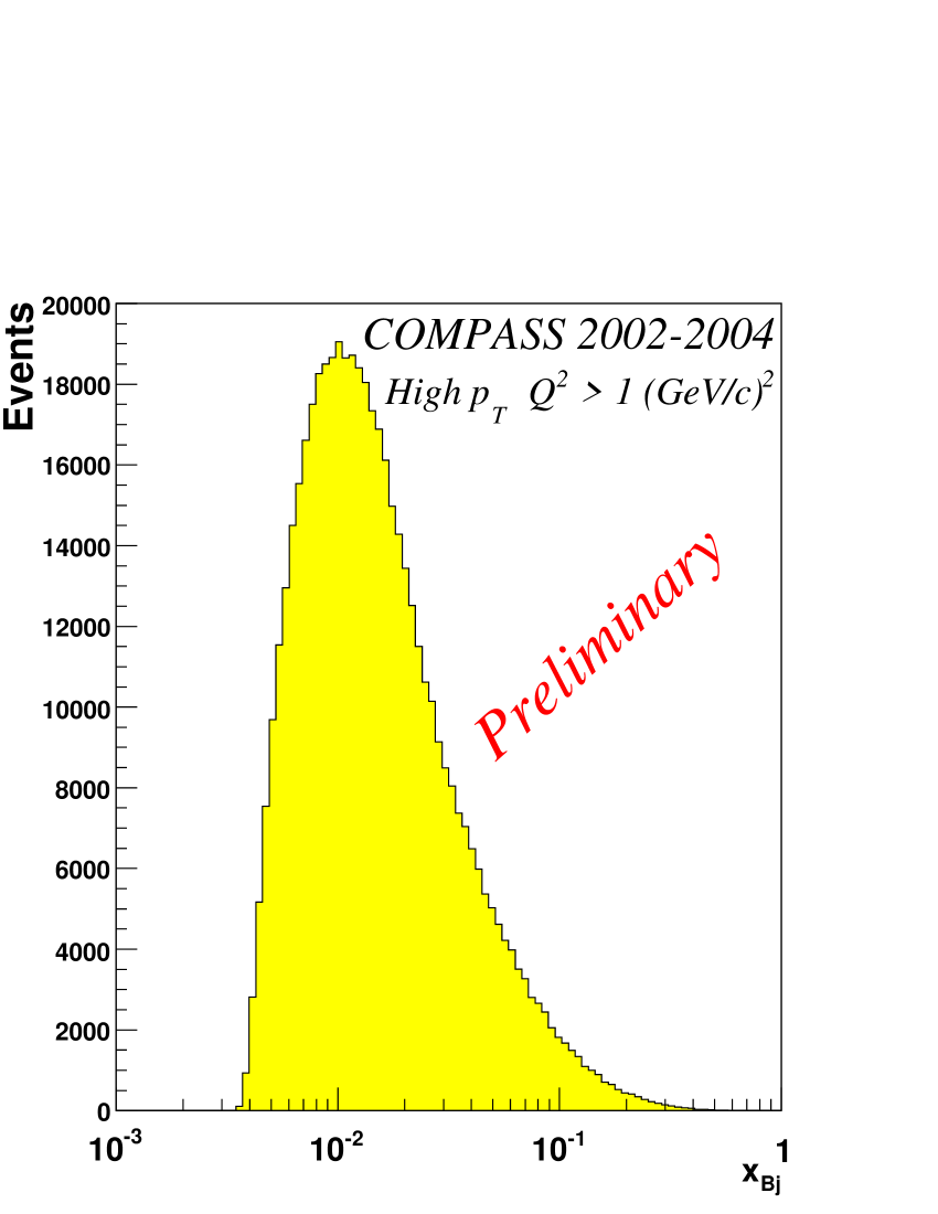
Figure 4: $Q^{2}$, $y$ and $x$ distributions of selected events.

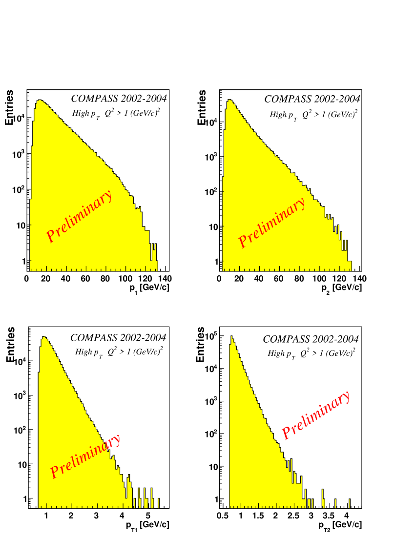
Figure 5: $p$ and $p_{T}$ distributions for leading and sub-leading hadrons: The left column shows the leading hadrons and the right column the sub-leading one. In the first row the momenta are plotted, in the second row the transverse momenta are shown.

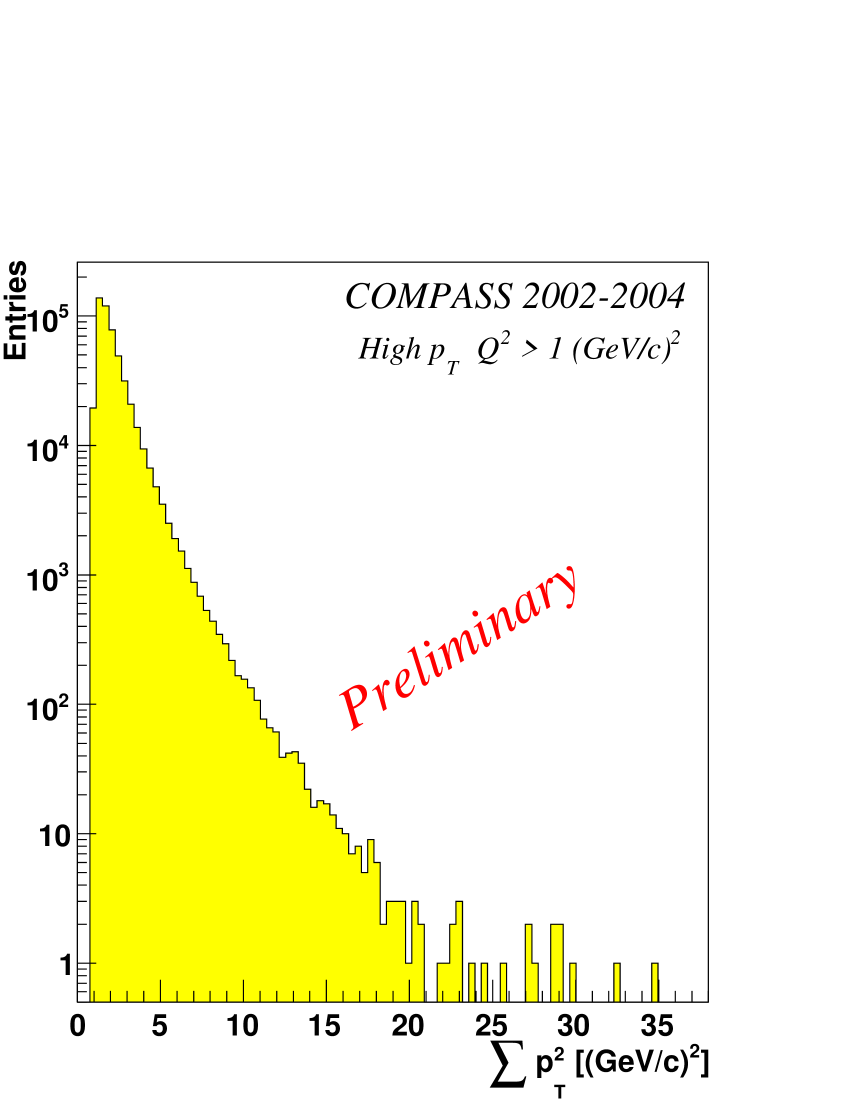
Figure 6: The distribution of the sum of the $p_{T}^{2}$ for the leading and sub-leading hadrons.

5 Monte Carlo simulation

A lot of information to be used in the $\Delta G/G$ calculation is obtained from Monte Carlo (MC) simulation, therefore this analysis is model dependent. That is the main reason why a good description of the experimental data by MC is fundamental in this analysis. Two MC samples were produced to account for the estimation of the statistical weight: one using the same cuts used in the high $p_{T}$ event selection in the previous section (sec. 4) and another using an inclusive selection based only on the cuts on the DIS kinematic variables ($Q^{2}$ and $y$). Both MC samples are restricted to the high $Q^{2}$ region. The MC production comprises three steps: First the events are generated, then a spectrometer simulation program is applied to these events and finally the events are reconstructed. The spectrometer simulation program based on GEANT3 geant was developed. The reconstruction procedure is the same for real and MC events.

For the first step the LEPTO 6.5 Ingelman:1996mq event generator is used together with a leading order parametrisation of the unpolarised parton distribution functions with partons generated in a fixed-flavour scheme given by MRST04LO Martin:2006qz , with a good description of $F_{2}$ in the COMPASS kinematic region. NLO corrections are simulated by the gluon radiation in the initial and final state (parton shower ON). The generation is done at two levels: the simulation of the hard scattering processes and the fragmentation and hadronisation model.

The fragmentation is based on the Lund string model Andersson:89 implemented in JETSET Sjostrand:2000wi . In this model the probability that a fraction $z$ of the available energy will be carried by a newly created hadron is expressed by the Lund symmetric function $f(z)=z^{-1}(1-z)^{a}e^{-bm_{\perp}/z}$, with $m_{\perp}^{2}=m^{2}+p_{\perp}^{2}$, where $m$ is the quark mass. To improve the agreement between MC and data, the parameters ($a$,$b$) were modified from their default values (0.3, 0.58) to (0.6, 0.1), and also the gluon radiation at the initial and final states were used; i.e. the so-called Parton Shower (PS) ON mode.

The transverse momentum of the hadrons, $k_{T}$, at the fragmentation level is given by the sum of the $p_{\perp}$ for $q_{i}\bar{q_{j}}$ hadron. Then the $k_{T}$ of the newly created hadrons is described by a convolution of two gaussian distributions; as it is illustrated in Fig. 7, PARJ(21) is the width of the narrower gaussian, PARJ(23) and PARJ(24) are, respectively, the factors to apply on the amplitude and on the width for the broader gaussian. The default values of (PARJ(21), PARJ(23), PARJ(24)) are (0.36 $(\mbox{GeV}/c)^{2}$, 0.01, 2.0), and were modified to (0.30 $(\mbox{GeV}/c)^{2}$, 0.02, 3.5). This set of modifications in these fragmentation parameters it is called the COMPASS tuning.

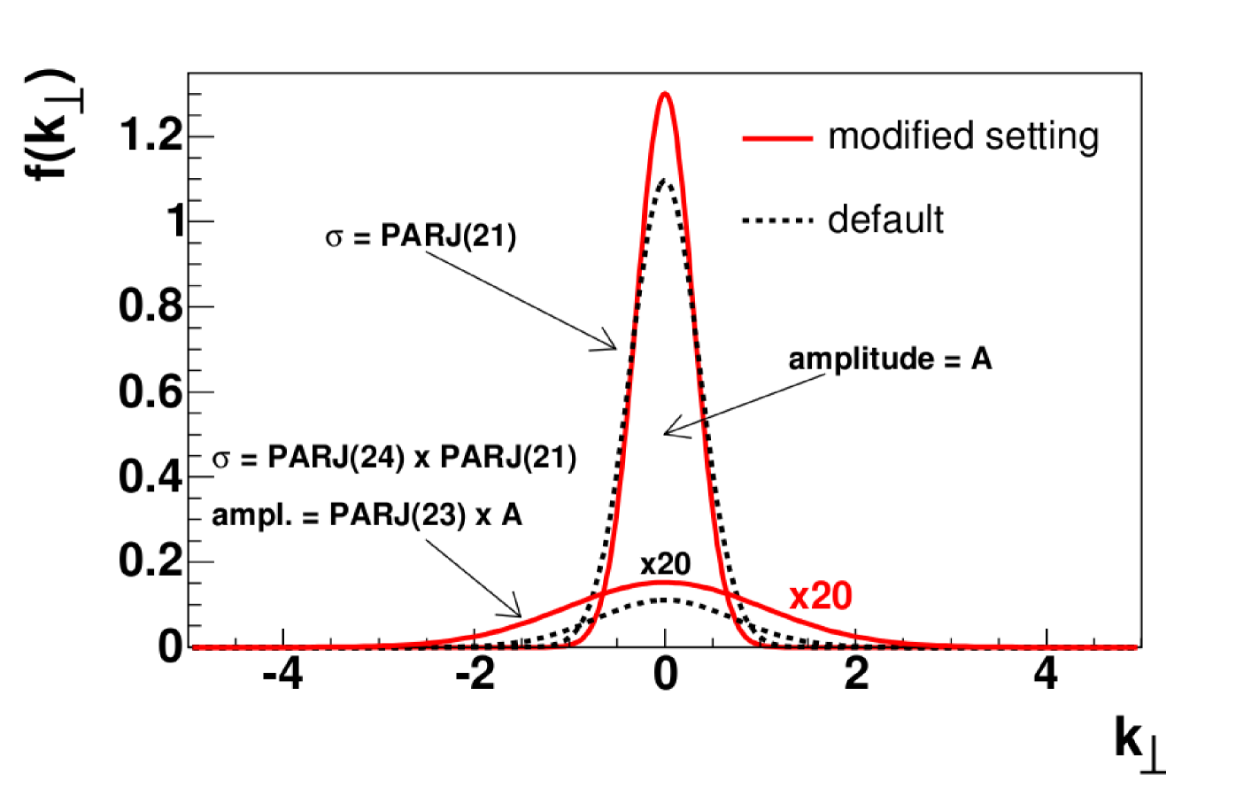
Figure 7: The distribution of $k_{T}$.

The remarkable agreement of the MC simulation with the data is illustrated in Figs. 8-10. In this analysis the used MC sample has PS on mode.

The MC–data comparison for different the kinematic variables is shown in Fig. 8. In Fig. 9 the hadronic variables, $p$, $p_{T}$ for the leading and sub-leading hadrons are shown, together with the sum of $p_{T}^{2}$; i.e. $\sum p_{T1}^{2}+p_{T2}^{2}$. In Fig. 10 the two comparison of the $\sum p_{T}^{2}$ variable one using the COMPASS tuning and another using the default LEPTO tuning is also shown the COMPASS tuning describes better our data sample than the LEPTO default one.

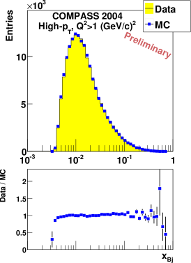
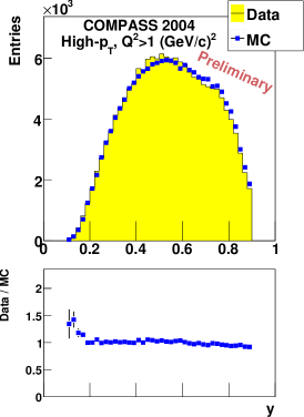
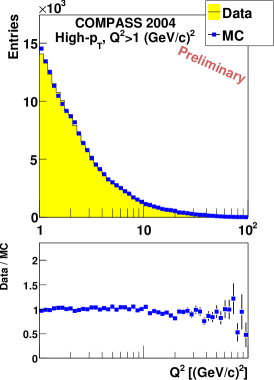
Figure 8: Comparison between data and MC simulation: On plots distributions and ratios Data/MC for inclusive variables are shown: $x_{Bj},\,Q^{2},\,y$.

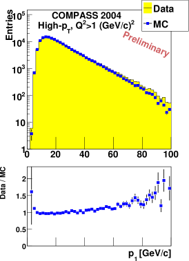
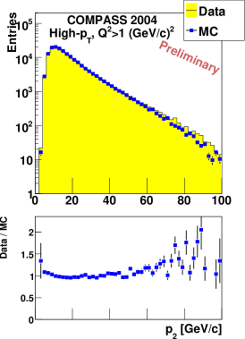
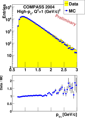
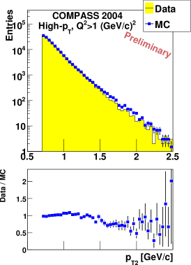
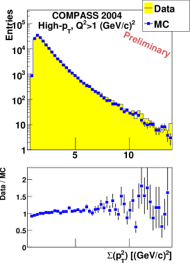
Figure 9: Comparison between data and MC simulation: On the plots distributions and ratios Data/MC for hadronic variables are shown: $p_{1},\,p_{2},\,p_{T1},\,p_{T2}$ and $\sum(p_{T}^{2}$.

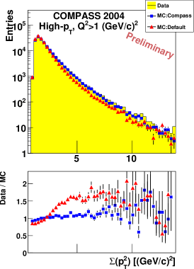
Figure 10: Comparison between COMPASS and default LEPTO MC genetation tunings for $\sum p_{T}^{2}$ variable.

6 The $\Delta G/G$ extracting method

The main goal of this approach is to enhance the PGF process which accounts for the gluon contribution to the nucleon spin. In the original idea of the high $p_{T}$ analysis, the selection was based on a very tight a set of cuts to suppress LO and QCD Compton. This situation results in a dramatic loss of statistics.

A new approach was found in which a not so strict set of cuts is applied, together with a neural network (NN) Sulej:2007zz to assign a probability to each event being originated from each of the three processes.

A parametrisation is created by the neural network using as input $x_{Bj}$ and $Q^{2}$, for inclusive sample and while for high $p_{T}$ sample the transverse and longitudinal momenta of the hadrons, namely $p_{T1}$, $p_{T2}$, $p_{l1}$, and $p_{l2}$, are used in addition. Using this parametrisation the values of the event fractions , $R$, the Bjorken variable, $x$ and the partonic asymmetry $a_{LL}$ for each process type are estimeted; these parameters represent the neural network output.

As the fractions of the three processes sum up to unity, we need two variables to parameterise them: $o_{1}$ and $o_{2}$. While for the remain output parameters are single.

The relations between the two neural network outputs $o_{1}$ and $o_{2}$ and the $R$ fraction are

• $R_{\rm PGF}=1-o_{1}-1/\sqrt{3}\cdot o_{2}$

• $R_{\rm QCDC}=o_{1}-1/\sqrt{3}\cdot o_{2}$

• $R_{\rm LO}=2/\sqrt{3}\cdot o_{2}$

A statistical weight is constructed for each event based on these probabilities. In this way we do not need to remove events that most likely do not came from PGF processes, because the weight will reduce their contribution in the gluon polarisation calculation. This approach uses wisely and optimally the statistical power of the available data.

To compute the gluon polarisation in an event-by-event basis the so-called 2nd order method jorg is used. In this analysis several neural networks are used.

The resulting neural network outputs for the fraction are presented in Fig. 11 in a 2-dimensional plot. The triangle limits the region where all fractions are positive. For the inclusive sample the average value of $o_{2}$ is quite large, which means that the LO process is the dominant one. The situation is different for the high $p_{T}$ sample, the average outputs are $\langle o_{1}\rangle\approx$ 0.5 and $\langle o_{2}\rangle\approx$ 0.35. Note also that the spread along $o_{2}$ is larger than along $o_{1}$.

This means that the neural network is able to detect a region where the contribution of PGF and QCDC is significant compared to LO; although it can not easily distinguish between the PGF and QCDC processes themselves.

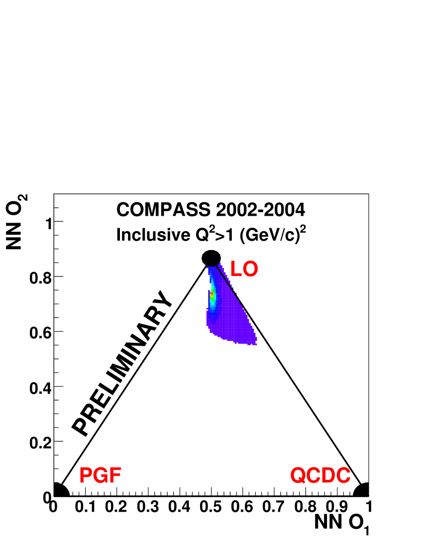
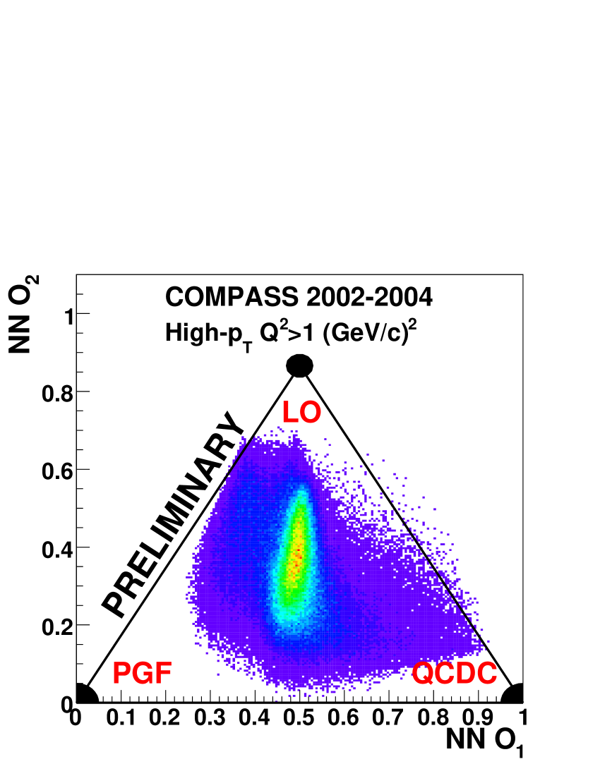
Figure 11: 2-d output of neural network for estimation that the given event is PGF, QCDC or LO; (left) for the inclusive sample and (right) for High $p_{T}$ sample.

For the inclusive sample, the $R$ fractions do not depend much upon $x_{Bj}$ and $Q^{2}$, there is no sharp cut, like e.g. PGF exists only for $12.5\ \mbox{GeV}/c^{2}<Q^{2}<15\ \mbox{GeV}/c^{2}$. Therefore the neural network, which gives the probability that a given event comes from PGF, QCDC or LO, never produces output close to $(0,0)$, i.e. $R_{\rm PGF}=1$. Instead all the inclusive events are confined in a quite limited region of $o_{1}$ and $o_{2}$. It is worth to note that the inclusive sample contains about 10% of PGF events.

To check the stability of the neural network the probability estimated from with the neural network is compared to the fraction of events for each process in MC. As can be seen it in Fig. 12, the comparisons are done for each process type separately and in bins of $\sum p_{T}^{2}$. The agreement for this comparison is good.

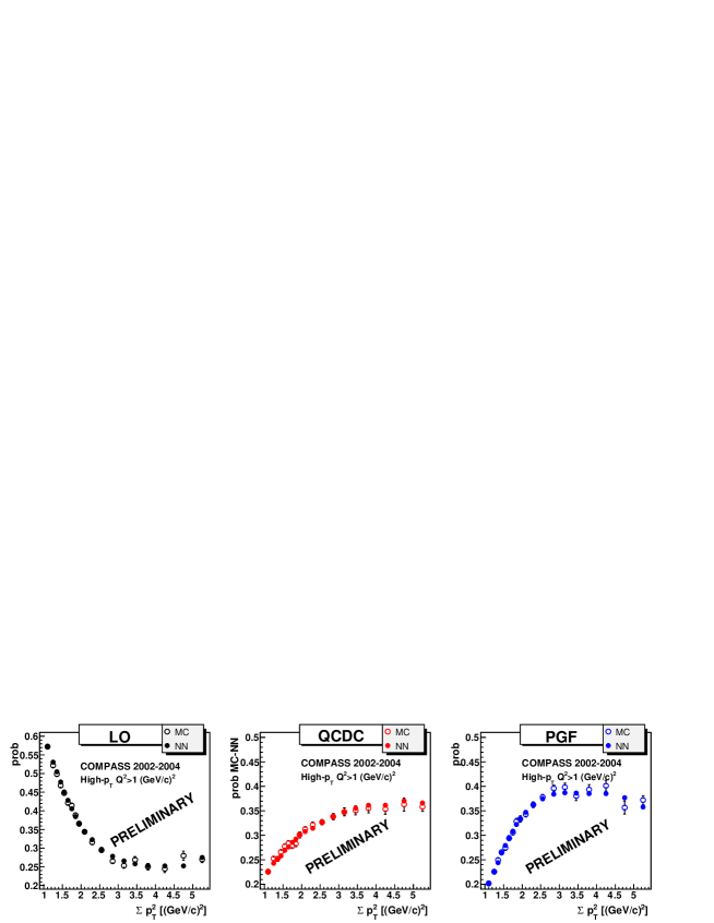
Figure 12: Neural network and MC comparison for $R_{\rm PGF}$, $R_{\rm QCDC}$, $R_{\rm LO}$as a function of $\sum p_{T}^{2}$.

7 High $p_{T}$ hadron pair analysis for low $Q^{2}$ region

This analysis was published in ref. Ageev:2005pq , using a data sample from the years 2002 to 2003. Here in this section, I will describe the same analysis but using data from 2002 to 2004.

The reason for splitting all the $Q^{2}$ range in two complementary regions is that for low $Q^{2}$ region the resolved photon contribution is considerably high ($\approx 50\ \%$). Therefore a more complicated description of the physics than pure QCD in lowest order needs to be included in the MC simulation.

This means that the analysis formalism, which is based on the processes that are involved in the analysis, is different for both regions. The data sample in the low $Q^{2}$ region is 90 % of all available data.

In the analysis in low $Q^{2}$ region the selection is essentially the same as in high $Q^{2}$ region plus a slightly tighter set of cuts: $x_{F}>0.1$, $z>0.1$, and $\sum p_{T}^{2}>2.5\ (\mbox{GeV}/c)^{2}$.

This strict set of cuts is used to reduce the physical background contributions (LO, QCD Compton and resolved photon). The weighting method used in the high $Q^{2}$ analysis, is not applied in this case. As a consequence not only the physical background is reduced but also a PGF fraction of events may be reduced too by this strict selection. In Fig. 13 the involved processes and their respective ratios are shown.

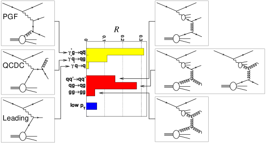
Figure 13: $Q^{2}$ distribution for the low $Q^{2}$ region.

The MC simulated and real data samples of high $p_{T}$ events are compared in Fig. 14 for $Q^{2}$, $y$, and for the total and transverse momenta of the leading hadron;showing a good agreement. An equally good agreement is obtained for the sub-leading hadron.

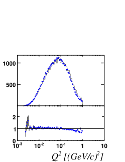
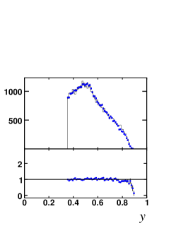
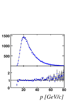
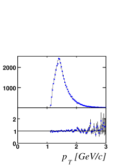
Figure 14: Comparison between data and MC for $Q^{2}$, $y$, and for the total (transverse) momentum $p$ ($p_{T}$) of the hadron with highest $p_{T}$. The upper part of each plot shows the real data (points) and simulation (line), normalised to the same number of events. The lower part shows the corresponding data/MC ratio.

The gluon polarisation in the low $Q^{2}$ region is extracted using averaged values as shown by this expression:

$$\left\langle\frac{A_{\rm LL}}{D}\right\rangle = R_{\rm PGF}\left\langle\frac{\hat{a}_{\rm LL}^{\rm PGF}}{D}\right\rangle\frac{\Delta G}{G}+R_{\rm QCDC}\left\langle\frac{\hat{a}_{\rm LL}^{\rm QCDC}}{D}A_{1}\right\rangle$$ (14)

$$+ \sum_{f,f^{\gamma}=u,d,s,\bar{u},\bar{d},\bar{s},G}R_{ff^{\gamma}}\left\langle\hat{a}_{\rm LL}^{ff^{\gamma}}\frac{\Delta f}{f}\frac{\Delta f^{\gamma}}{f^{\gamma}}\right\rangle$$

$$+ R_{\rm LO}\times A_{\rm LO}+R_{\rm low-p_{T}}\times A_{\rm low-p_{T}}.$$

The hard scale used to compute the gluon polarisation is set by the $p_{T}^{2}$ of the hadrons.

Here, $R_{ff^{\gamma}}$ is the fraction of events in the whole high $p_{T}$ sample for which a parton $f$ from the nucleon interacts with a parton $f^{\gamma}$ from a resolved photon. $A_{1}$ is the inclusive virtual photon deuteron asymmetry. $\Delta f/f$ ($\Delta f^{\gamma}/f^{\gamma}$) is the polarisation of quarks or gluons in the deuteron (photon). $R_{\rm low-p_{T}}$ and $A_{\rm low-p_{T}}$ are respectively the fraction and the asymmetry for events for which no hard scale can be found, these events are classified in PYTHIA as “low-$p_{T}$” processes. However the asymmetry for this kind of events is small, as indicated by previous measurements of $A_{1}$ at low $Q^{2}$ Adeva:1999pa . Moreover, the leading and low-$p_{T}$ processes together account for only 7% of the high $p_{T}$ sample. For these two reasons, we neglected their contributions.

The PGF analysing power $\hat{a}_{\rm LL}^{\rm PGF}$ is calculated using the leading order expressions for the polarised and unpolarised partonic cross sections and the parton kinematics for each PGF event in the high $p_{T}$ MC sample.

The contribution of QCD Compton events to the high $p_{T}$ asymmetry is evaluated from a parametrisation of the virtual photon deuteron asymmetry $A_{1}$ based on a fit to the world data Adeva:1998vv ; Abe:1998wq . This asymmetry is calculated for each event at the momentum fraction $x_{\rm q}$ of the quark, known in the simulation.

The parton from a resolved photon interacts either with a quark or a gluon from the nucleon. In the latter case, the process is sensitive to the gluon polarisation $\Delta G/G$. The analysing powers $\hat{a}_{\rm LL}^{ff^{\gamma}}$ are calculated in pQCD at leading order Bourrely:1987gp . The polarisations of the $u$, $d$ and $s$ quarks in the deuteron $\Delta f/f$ are calculated using the polarised parton distribution functions from Ref. Gluck:2000dy (GRSV2000) and the unpolarised parton distribution functions from Ref. Gluck:1998xa (GRV98, also used as an input for PYTHIA), all at leading order. The polarisations of quarks and gluons in the virtual photon $\Delta f^{\gamma}/f^{\gamma}$ are unknown because the polarised parton distribution functions of the virtual photon have not yet been measured. Nevertheless, theoretical considerations provide a minimum and a maximum value for each $\Delta f^{\gamma}$, in the so-called minimal and maximal scenarios Gluck:2001rn .

8 Results

The preliminary measurements of the gluon polarisation in low and high $Q^{2}$ regions, using data from the years 2002 to 2004, are:

$$\left(\Delta G/G\right)_{{\rm low}\ Q^{2}} = 0.02\pm 0.06_{(stat.)}\pm 0.06_{(syst.)}\qquad{\rm with}\quad x_{G}=0.09^{+0.07}_{-0.04}$$

$$\left(\Delta G/G\right)_{{\rm high}\ Q^{2}} = 0.08\pm 0.10_{(stat.)}\pm 0.05_{(syst.)}\qquad{\rm with}\quad x_{G}=0.08^{+0.04}_{-0.03}$$

The average of the hard scale, $\mu^{2}$, for low and high $Q^{2}$ is 3 $(\mbox{GeV}/c)^{2}$. $x_{G}$ is the momentum fraction carried by the probed gluons and it is determined by the $x_{Bj}$ distribution for the PGF processes, obtained from the MC parton kinematics.

The published result of this measurement for low $Q^{2}$ using data from 2002 to 2003 can be found in this ref. Ageev:2005pq . while for the low $Q^{2}$ measurement obtained using data from 2002 to 2004 was presented in several conferences, therefore this result is presented for comparison with the high $Q^{2}$ one.

Concerning the systematic error related to the gluon polarisation in the high $Q^{2}$ region several studies were performed to estimate its value.

For the neural network contribution to the systematic error, several neural networks with different fixed number of neurons in their internal structure were trained on the same MC sample, and for each $\Delta G/G$ was extracted.

For the MC contribution several tests were performed with different fragmentation and initial and final gluon radiation.

The relative error of $\delta P_{b}$, $\delta P_{t}$ is taken as 5% and 2% for relative error of the dilution factor, $\delta f/f$. It is assumed that the systematic error of $\delta(\Delta G/G)_{fP_{b}P_{t}}$ is proportional to the errors given above.

The false asymmetries are extracted using several constraints in the spectrometer with the purpose to assess its stability. Two main issues have a significant contribution to the false asymmetries. The first one is related to the asymmetry computed using acquired data from positive and negative microwave configurations separately. The second issue is related to the asymmetry calculated form different regions of the spectrometer (top, bottom, left and right regions).

A world data fit, with all $Q^{2}$ range, compassrho is used to parametrise $A_{1}^{d}$, to extract the preliminary value of $\Delta G/G$. Four different parameterisations of $A_{1}^{d}$ are used to estimate the associated systematics.

The impact of the $x^{\prime}_{C}$ factor in the eq. (12) was estimated in a two tests. In the first one $x^{\prime}_{C}$ was assumed to be proportional to $x_{C}$. In the second $x^{\prime}_{C}$ was approximated by using $x_{C}$ instead of $x_{Bj}$ as an input parameter for the neural network which estimates $x_{C}$.

The main contributions to this uncertainty are summarised in Table 2 together with their estimated values.

$\delta(\Delta G/G)_{NN}$	0.006
$\delta(\Delta G/G)_{MC}$	0.040
$\delta(\Delta G/G)_{f,P_{b},P_{t}}$	0.006
$\delta(\Delta G/G)_{false}$	0.011
$\delta(\Delta G/G)_{A1^{d}}$	0.008
$\delta(\Delta G/G)_{formula}$	0.013
TOTAL	0.045

Table 2: Summary of the major systematic contributions

9 Conclusions and outlook

The preliminary values of the gluon polarisation for low and high $Q^{2}$ regions were presented. The gluons were probed at an average scale $\langle\mu^{2}\rangle\approx 3\ (\mbox{GeV/}c)^{2}$.

Fig. 15 shows these new values of $\Delta G/G$ together with the preliminary value from the open charm analysis comp.del_sigma and the measurements from SMC collaboration, from the high $p_{T}$ analysis for the $Q^{2}>1\ (\mbox{GeV/}c)^{2}$ region Adeva:2004dh and also the measurements from HERMES collaboration; for single hadrons and high $p_{T}$ hadrons pairs analyses Airapetian:1999ib . The curves in Fig. 15 are the parametrisation of $\Delta G/G(x)$ using a NLO QCD analysis in the $\overline{MS}$ scheme with a renormalisation scale $\langle\mu^{2}\rangle=3\ (\mbox{GeV/}c)^{2}$. The curve with the dashed line is the QCD fit assuming that $\Delta G>0$, the dotted line is the QCD fit assuming $\Delta G<0$. It is seen that both high $p_{T}$ values; for high and low $Q^{2}$ analyses are in compatible with each other and also, within their $x_{G}$ region, in agreement with the NLO QCD fits. These both measurement show that gluon contribution to the spin for $x_{G}\approx 0.1$ is compatible with zero.

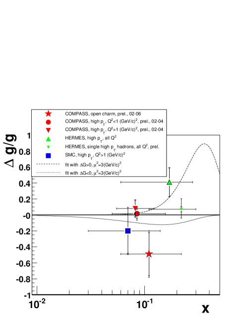
Figure 15: Comparison of $\Delta G/G$ measurements from COMPASS comp.del_sigma , SMC Adeva:2004dh , and HERMES Airapetian:1999ib . The two curves correspond to the parametrisation from the NLO QCD analysis in the $\overline{MS}$ scheme with scale at 3 $(\mbox{GeV/}c)^{2}$

References

- (1) M. J. Alguard et al., Phys. Rev. Lett. 37 (1976) 1261.
- (2) G. Baum et al., Phys. Rev. Lett. 51 (1983) 1135.
- (3) J. R. Ellis and R. L. Jaffe, Phys. Rev. D 9 (1974) 1444 [Erratum-ibid. D 10 (1974) 1669].
-
(4)
J. Ashman et al. [European Muon Collaboration],
Phys. Lett. B 206 (1988) 364.
J. Ashman et al. [European Muon Collaboration], Nucl. Phys. B 328 (1989) 1. - (5) K. Abe et al. [E154 Collaboration], Phys. Rev. Lett. 79 (1997) 26 [arXiv:hep-ex/9705012].
- (6) K. Abe et al. [E143 collaboration], Phys. Rev. D 58, (1998) 112003 [arXiv:hep-ph/9802357].
- (7) P. L. Anthony et al. [E142 Collaboration], Phys. Rev. D 54, (1996) 6620 [arXiv:hep-ex/9610007].
- (8) P. L. Anthony et al. [E155 Collaboration], Phys. Lett. B 458 (1999) 529 [arXiv:hep-ex/9901006].
- (9) D. Adams et al. [Spin Muon Collaboration (SMC)], Phys. Rev. D 56 (1997) 5330 [arXiv:hep-ex/9702005].
- (10) A. Airapetian et al. [HERMES Collaboration], Phys. Lett. B 442 (1998) 484 [arXiv:hep-ex/9807015].
- (11) V. Y. Alexakhin et al. [COMPASS Collaboration], Phys. Lett. B 647 (2007) 8.
- (12) M. Alekseev et al. [COMPASS collaboartion], Eur. Phys. J. C 52 (2007) 255.
- (13) A. Abragam, The Principles of nuclear magnetism (The Clarendon Press , Oxford, 1961).
- (14) P. Abbon et al., Nuclear Instruments and Methods in Physics Research A577 (2007) 455.
- (15) R. Brun et al., CERN Program Library W5013 (1994).
- (16) G. Ingelman, A. Edin and J. Rathsman, Comput. Phys. Commun. 101 (1997) 108 [arXiv:hep-ph/9605286].
- (17) A. D. Martin, W. J. Stirling and R. S. Thorne, Phys. Lett. B 636 (2006) 259 [arXiv:hep-ph/0603143].
- (18) B. Andresson, The Lund model (Cambridge Univ. Press , Cambridge, 1989).
- (19) T. Sjostrand, P. Eden, C. Friberg, L. Lonnblad, G. Miu, S. Mrenna and E. Norrbin, Comput. Phys. Commun. 135 (2001) 238 [arXiv:hep-ph/0010017].
- (20) R. Sulej, K. Zaremba, K. Kurek and E. Rondio, Measur. Sci. Tech. 18 (2007) 2486.
- (21) J. Pretz, “A New Method for Asymmetry Extraction”, COMPASS internal note (2004).
- (22) E. S. Ageev et al. [COMPASS Collaboration], Phys. Lett. B 633 (2006) 25 [arXiv:hep-ex/0511028].
- (23) B. Adeva et al. [SMC], Phys. Rev. D 60 (1999) 072004.
- (24) B. Adeva et al. [SMC], Phys. Rev. D 58 (1998) 112001.
- (25) C. Bourrely, J. Soffer, F. M. Renard, and P. Taxil, Phys. Rept. 177 (1989) 319.
- (26) M. Glück, E. Reya, M. Stratmann, and W. Vogelsang, Phys. Rev. D 63 (2001) 094005.
- (27) M. Glück, E. Reya, and A. Vogt, Eur. Phys. J. C 5 (1998) 461.
- (28) M. Glück, E. Reya, and C. Sieg, Eur. Phys. J. C 20 (2001) 271.
- (29) B. Adeva et al. [SMC], Phys. Rev. D 70 (2004) 012002.
- (30) A. Airapetian et al. [HERMES collaboration], Phys. Rev. Lett. 84 (2000) 2584.