Probing Capacity

Abstract

We consider the problem of optimal probing of states of a channel by transmitter and receiver for maximizing rate of reliable communication. The channel is discrete memoryless (DMC) with i.i.d. states. The encoder takes probing actions dependent on the message. It then uses the state information obtained from probing causally or non-causally to generate channel input symbols. The decoder may also take channel probing actions as a function of the observed channel output and use the channel state information thus acquired, along with the channel output, to estimate the message. We refer to the maximum achievable rate for reliable communication for such systems as the ‘Probing Capacity’. We characterize this capacity when the encoder and decoder actions are cost constrained. To motivate the problem, we begin by characterizing the trade-off between the capacity and fraction of channel states the encoder is allowed to observe, while the decoder is aware of channel states. In this setting of ‘to observe or not to observe’ state at the encoder, we compute certain numerical examples and note a pleasing phenomenon, where encoder can observe a relatively small fraction of states and yet communicate at maximum rate, i.e. rate when observing states at encoder is not cost constrained.

I Introduction

Shannon showed the importance of availability of channel state at the encoder for communication system in his seminal paper [1], where he computed capacity of DMC with i.i.d. states available causally to the encoder. This spawned an active research in the area of channel coding and was extended to various scenarios, notably for storage in computer memory. Kuznetsov and Tsybakov in [2] constructed defect-correcting codes for coding in computer memory with defective cells. Gel’fand and Pinsker in [3], extended work in [1] to the case where channel states are available non-causally to the encoder, again with applications for computer memories, which was further researched by Heegard and El Gamal in [4]. Keshet, Steinberg and Merhav presented a detailed survey in [5] on channel coding in the presence of state information, where the channel state information (CSI) signal is available at the transmitter (CSIT) or at the receiver (CSIR), or both.

Permuter and Weissman introduced the notion of actions in source coding context in [6]. Their setting is a generalization of the Wyner-Ziv source coding with decoder side information problem ([7]), where now the decoder can take actions based on the index obtained from the encoder to affect the formation or availability of side information. Weissman, in [8], studied the channel coding dual where the transmitter takes actions that affect the formation of channel states. This framework captures various new coding scenarios which include two stage recording on a memory with defects, motivated by similar problems in magnetic recording and computer memories. Kittichokechai et al in [9] studied a variant of the problem in [6] and [8], where encoder and decoder both have action dependent partial side information. However, in the source coding formulation of [6], they restricted the actions to be taken by decoder while in the channel coding scenario of [8] and [9], actions were taken only by the encoder.

In this paper, we revisit channel coding scenarios but now cost constrained actions are taken to acquire any partial or complete channel state information by the encoder, the decoder or both. Our framework is aimed at capturing and understanding the trade offs involved in natural scenarios where the acquisition of channel state information is associated with expenditure of costly system resources. The encoder and decoder actions are cost constrained creating tension between achievable rate and the cost of acquisition of the channel state (or the defect) information. Note that our framework differs from those of [8] and [9] where actions affect the channel, followed by channel encoding. In our scenario channel statistics are not affected, i.e., nature generates the state sequence i.i.d $\sim P_{S}$. Our work is novel in the sense that not only the encoder but the decoder also takes actions to acquire channel state information. Encoder takes actions ($A_{e}$) depending on messages. Decoder also takes actions ($A_{d}$) depending upon observed channel output. Using their respective actions, encoder and decoder observe partial states, $S_{e}$ and $S_{d}$ through discrete memoryless channel (DMC), $P_{S_{e},S_{d}|S,A_{e},A_{d}}$. The encoder can causally or non-causally use its partial state information to generate the channel input symbols. In this paper, we characterize the fundamental limit of such a framework and call it Probing Capacity. When the actions are not taken by the decoder, there is an equivalence between our setting and that of channels with action dependent states as in [8], which we make explicit in Section III.

The rest of the paper is organized as follows. We begin with a motivating scenario in Section II, where decoder knows the complete state and the encoder takes message dependent binary actions to observe or not to observe the channel state. This is generalized in Section III, when only encoder takes actions. This section also establishes the equivalence between our framework of optimal probing and that of channels with action dependent states in [8]. Motivated by the framework of communication over slow fading channels, where the information of channel states is to be exploited on the fly, we have in Section IV characterization of the probing capacity where encoder takes actions to get channel states and use them causally to construct channel inputs and decoder takes actions strictly causally dependent on channel outputs. Note that in this section, we characterize a novel and a generalized setting, where both encoder and decoder take costly actions to get channel state information. Later in this section, inspired by coding on computer memory with defects, we explain the non-causal case, i.e., when channel states are used non-causally by the encoder to generate channel input symbols and decoder waits for the entire channel output before taking actions to get channel states. This in general is a hard problem and we show its equivalence to a standard relay channel with infinite lookahead. In Section V, we work out several examples, with some surprising implications. The paper is concluded in Section VI with directions of future research.

II To Observe or Not to Observe Channel States at Encoder

We begin by explaining the notation to be used throughout this paper. Let upper case, lower case, and calligraphic letter denote, respectively, random variables, specific or deterministic values which random variables may assume, and their alphabets. For two jointly distributed random variables, $X$ and $Y$, let $P_{X}$, $P_{XY}$ and $P_{X|Y}$ respectively denote the marginal of $X$, joint distribution of $(X,Y)$ and conditional distribution of $X$ given $Y$. $X_{m}^{n}$ is a shorthand for $n-m+1$ tuple $\{X_{m},X_{m+1},\cdots,X_{n-1},X_{n}\}$. We impose the assumption of finiteness of cardinality on all alphabets, unless otherwise indicated.

In this section, we consider the problem of optimal probing where encoder takes a ‘costly’ action depending upon message and use it to probe the channel and observe or not the channel state. The actions are binary, hence while action, $A=1$ corresponds to the case when encoder observes the channel state, action, $A=0$ implies no acquired state information. Note that such a kind of abstraction taps in the motivation considered in Compressed Sensing framework in [10], where due to cost of sensing and measurement, you aim to observe only a few noisy signal observations and construct the original signal accurately. We further assume decoder knows the complete state information and that the encoder uses partial state information non-causally to generate channel input symbol.

II-A Problem Setup

The setting is depicted in Figure 1: Message $M$ is selected uniformly from a uniform distribution on the message set $\mathcal{M}=\{1,2,\cdots,\left|\mathcal{M}\right|\}$. Nature generates states sequence $S^{n}\in\mathcal{S}^{n}$ i.i.d $\sim P_{S}$, independent of message. A $(2^{nR},n)$ code consists of :

• Probing Logic : $f_{A}:M\rightarrow A^{n}\in\{0,1\}^{n}$ such that the action sequence $A^{n}$ satisfies the cost constraints

  $$\Lambda(A^{n})=\frac{1}{n}\sum_{i=1}^{n}\Lambda(A_{i})\leq\Gamma,$$ (1)

  where $\Lambda(\cdot)$ is the cost function while $\Gamma$ is the cost constraint. Given nature generated state sequence $S^{n}$ and message dependent action sequence $A^{n}$, encoder receives partial state information $S_{e}^{n}\in\{\{\ast\}\cup\mathcal{S}\}^{n}$ through a deterministic channel characterized by,

  $$S_{e}=h(S,A)=S\mbox{ if }A=1,$$ (2)

  $$S_{e}=h(S,A)=\ast\mbox{ if }A=0,$$ (3)

  where $\ast$ stands for erasure or no information of state symbol. Thus, $A=1$ corresponds to an observation of the channel state while $A=0$ to a lack of an observation. Without loss of generality we can assume, $\Gamma(0)=0$.

• Encoding : $f_{e}:(M,S^{n}_{e})\rightarrow X^{n}\in\mathcal{X}^{n}$, i.e. encoder uses the partial state information non-causally to generate channel input symbols.

• Decoding : $f_{d}:(Y^{n},S^{n})\rightarrow\hat{M}\in\mathcal{\{}1,2,\cdots,\left|\mathcal{M}\right|\}$, where the channel output $Y^{n}\in\mathcal{Y}^{n}$.

The joint PMF on $(M,A^{n},S^{n},S^{n}_{e},X^{n},Y^{n},\hat{M})$ induced by a given scheme is

$$P_{M,A^{n},S^{n},S^{n}_{e},X^{n},Y^{n},\hat{M}}(m,a^{n},s^{n},s^{n}_{e},x^{n},y^{n},\hat{m})$$ (4)

$$= \frac{{\bf 1}_{\{f_{A}(m)=a^{n},f_{e}(m,s_{e}^{n})=x^{n},f_{d}(y^{n},s^{n})=\hat{m}\}}}{\left|\mathcal{M}\right|}\prod_{i=1}^{n}P_{S}(s_{i}){\bf 1}_{\{s_{e,i}=h(s_{i},a_{i})\}}P_{Y|X,S}(y_{i}|x_{i},s_{i}).$$

The probability of error is calculated as $P_{e}=P(M\neq\hat{M}(Y^{n},S^{n}))$. The rate $R$ is said to be achievable if there exists a sequence of $(2^{nR},n)$ codes for increasing block lengths satisfying the cost constraints (1) with $\frac{1}{n}\log\left|\mathcal{M}\right|\leq R$ and $P^{n}_{e}\stackrel{{\scriptstyle n\rightarrow\infty}}{{\longrightarrow}}0$

Figure 1: Encoder takes message dependent actions to observe state, encodes using available partial state information non-causally while decoder knows the complete channel state sequence.

II-B Probing Capacity

Theorem 1

The cost constrained ‘probing capacity’ of the system in Fig. 1 with channel inputs constructed using the observed state sequence non-causally while decoder has complete information of the state is given by

$$C(\Gamma)=\max[I(X;Y|S)],$$ (5)

where maximization is over all joint distributions of the form

$$P_{A,S,S_{e},X,Y}=P_{A}P_{S}{\bf 1}_{\{S_{e}=h(S,A)\}}P_{X|S_{e},A}P_{Y|X,S},$$ (6)

for some $P_{A},P_{X|S_{e},A}$ such that $E[\Lambda(A)]\leq\Gamma$.

Proof:

Achievability : We use Rate-Splitting and Multiplexing to achieve capacity (for a similar scheme refer to [11]). Note that in this problem while knowing $S_{e}$ we know $A$, hence we would show achievability with $P_{X|S_{e},A}$ replaced by $P_{X|S_{e}}$. Without loss of generality we assume $\mathcal{S}=\{1,2,\cdots,\left|\mathcal{S}\right|\}$, hence $\mathcal{S}_{e}=\{\ast,1,2,\cdots,\left|\mathcal{S}\right|\}$. Fix $P_{A},P_{X|S_{e}}$ which achieve $C(\frac{\Gamma}{1+\epsilon})$. We split message $M$ of rate $R$ into two messages $M_{1}$ and $M_{2}$ of rate $R_{1}$ and $R_{2}$ respectively.

• Generation of Codebooks :

  • Generate codebook $\mathcal{C}_{A}$ of $\{A^{n}(m_{1})\}_{m_{1}=1}^{2^{nR_{1}}}$ $n$-tuples i.i.d. $\sim P_{A}$. To send message $M=(M_{1},M_{2})$, if $A^{n}(M_{1})\in T^{n}_{\epsilon}(A)$ ($T_{\epsilon}^{n}$ are typical in the sense of [12]), then action $A^{n}(M_{1})$ is taken, else $A_{0}^{n}=(0,0,\cdots,0)$ is taken. If $A^{n}(M_{1})\in T^{n}_{\epsilon}(A)$, then by typical average lemma [13], constraints are satisfied as,

    $$\Lambda(A^{n})=\frac{1}{n}\sum_{i=1}^{n}\Lambda(A_{i})\leq(1+\epsilon)E(\Lambda(A))=\Gamma.$$ (7)

  • For every $A^{n}(m_{1})$, generate a codebook $\mathcal{C}_{X}(m_{1})$ of $\{(X_{e}^{n}(m_{1},m_{2}),X_{1}^{n}(m_{1},m_{2}),\cdots,X_{\left|\mathcal{S}\right|}^{n}(m_{1},m_{2}))\}_{m_{2}=1}^{2^{nR_{2}}}$
    $(\left|\mathcal{S}\right|+1)n$-tuples such that $X_{e}^{n}$, $X_{1}^{n},\cdots,X_{\left|\mathcal{S}\right|}^{n}$ are i.i.d. $\sim P_{X|S_{e}=\ast},P_{X|S_{e}=1},\cdots,P_{X|S_{e}=\left|\mathcal{S}\right|}$ respectively. Also generate a codebook $\mathcal{C}^{0}_{X}$ of codewords $\{(X_{0,e}^{n}(m_{2})\}_{m_{2}=1}^{2^{nR_{2}}}$ i.i.d. $\sim P_{X|S_{e}=\ast}$.

• Encoding :

  • Given a message $M=(M_{1},M_{2})$, encoder decides to take actions $A^{n}(M_{1})$ or $A^{n}_{0}$ depending whether $A^{n}(M_{1})$ is in $T^{n}_{\epsilon}(A)$ or not. If $A^{n}(M_{1})\in T^{n}_{\epsilon}(A)$ encoder finds $S_{e}^{n}=h(A^{n}(M_{1}),S^{n})$, and then sends $X^{n}(M_{1},M_{2})$ using the following multiplexing.

    $$X_{i} = X_{e,i}(M_{1},M_{2})\mbox{ if }S_{e,i}=\ast,$$ (8)

    $$X_{i} = X_{j,i}(M_{1},M_{2})\mbox{ if }S_{e,i}=j\in\{1,2,\cdots,\left|\mathcal{S}\right|\}.$$

    If $A^{n}(M_{1})\notin T^{n}_{\epsilon}(A)$, encoder sends $X^{n}_{0}(M_{2})$.

• Decoding : We perform Successive Decoding and Demultiplexing. By successive decoding we mean that actions are decoded first by decoder and then the actual codewords.

  • On obtaining the channel output sequence $Y^{n}$ and channel state sequence $S^{n}$ decoder finds the smallest value of $\hat{M}_{1}$ for which $(A^{n}(\hat{M}_{1}),Y^{n},S^{n})\in T_{\epsilon}^{n}(A,Y,S)$. If there is no such $\hat{M_{1}}$, decoder assumes $\hat{M}_{1}=1$.

  • Once the decoder decodes the value of $M_{1}$, if $A^{n}(M_{1})\in T^{n}_{\epsilon}(A)$, it knows $S^{n}_{e}=h(A^{n}(M_{1}),S^{n})$ and hence, using the codebook $C_{X}(M_{1})$, it demultiplexes $\{(X_{e}^{n}(M_{1},m_{2}),X_{1}^{n}(M_{1},m_{2}),\cdots,X_{\left|\mathcal{S}\right|}^{n}(M_{1},m_{2}))\}_{m_{2}=1}^{2^{nR_{2}}}$ to construct $X^{n}(M_{1},m_{2})_{m_{2}=1}^{2^{nR_{2}}}$ sequences as,

    $$X_{i}(M_{1},m_{2}) = X_{e,i}(M_{1},m_{2})\mbox{ if }S_{e,i}=\ast,$$ (10)

    $$X_{i}(M_{1},m_{2}) = X_{j,i}(M_{1},m_{2})\mbox{ if }S_{e,i}=j\in\{1,2,\cdots,\left|\mathcal{S}\right|\}.$$ (11)

  • After demultiplexing, if $A^{n}(M_{1})\in T^{n}_{\epsilon}(A)$, decoder finds the smallest value of $\hat{M_{2}}$ for which $(X^{n}(M_{1},\hat{M}_{2}),Y^{n}|S^{n},A^{n}(M_{1}))\in T_{\epsilon}^{n}(X,Y|S^{n},A^{n}(M_{1})$. If there is no such $\hat{M_{2}}$, decoder assumes $\hat{M_{2}}=1$. If $A^{n}(M_{1})\notin T^{n}_{\epsilon}(A)$, decoder finds the smallest value of $\hat{M_{2}}$ for which $(X_{0}^{n}(\hat{M}_{2}),Y^{n}|S^{n})\in T_{\epsilon}^{n}(X,Y|S^{n})$, else $\hat{M_{2}}=1$ is assumed.

• Analysis of Probability of Error : Without loss of generality we can assume $M=(M_{1},M_{2})=(1,1)$ was sent. We have the following error events,

  • $\mathcal{E}_{11}=\{A^{n}(1),Y^{n},S^{n}\}\notin T_{\epsilon}^{n}(A,Y,S)$.

  • $\mathcal{E}_{12}=\{A^{n}(\hat{m}_{1}),Y^{n},S^{n}\}\in T_{\epsilon}^{n}(A,Y,S)$ for $\hat{m}_{1}\neq 1$.

  • $\mathcal{E}_{21}=\{X^{n}(1,1),Y^{n}|S^{n},A^{n}(1)\}\notin T_{\epsilon}^{n}(X,Y|S^{n},A^{n}(1))$.

  • $\mathcal{E}_{22}=\{X^{n}(1,\hat{m}_{2}),Y^{n}|S^{n},A^{n}(1)\}\in T_{\epsilon}^{n}(X,Y|S^{n},A^{n}(1))$ for $\hat{m}_{2}\neq 1$.

  Let $\mathcal{E}_{0}=P((A^{n}(1),X^{n}(1,1))\in T^{n}_{\epsilon}(A,X))$. Hence,

  $$P(\mathcal{E}) = P(\mathcal{E}_{0}\cap\mathcal{E})+P(\mathcal{E}^{c}_{0}\cap\mathcal{E})$$ (12)

  $$\leq P(\mathcal{E}_{0}\cap\mathcal{E})+P(\mathcal{E}^{c}_{0}).$$ (13)

  Note that by LLN ([13]), $P(\mathcal{E}^{c}_{0})\rightarrow 0$ as $n\rightarrow\infty$.
  We will now show that $P(\mathcal{E}_{0}\cap\mathcal{E})\rightarrow 0$. Let $\mathcal{E}_{1}=\mathcal{E}_{11}\cup\mathcal{E}_{12}$ and $\mathcal{E}_{2}=\mathcal{E}_{21}\cup\mathcal{E}_{22}$. By Law of Large Numbers, (LLN, ([13]), $P(\mathcal{E}_{0}\cap\mathcal{E}_{11})\rightarrow 0$. By Packing Lemma ([13]), $P(\mathcal{E}_{0}\cap\mathcal{E}_{12})\rightarrow 0$ if $R_{1}<I(A;Y,S)=I(A;Y|S)$ which implies by union bound $P(\mathcal{E}_{0}\cap\mathcal{E}_{1})\leq P(\mathcal{E}_{0}\cap\mathcal{E}_{11})+P(\mathcal{E}_{0}\cap\mathcal{E}_{12})\rightarrow 0$.
  Similarly by LLN, $P(\mathcal{E}_{0}\cap\mathcal{E}^{c}_{1}\cap\mathcal{E}_{21})\rightarrow 0$ and by Packing Lemma $P(\mathcal{E}_{0}\cap\mathcal{E}^{c}_{1}\cap\mathcal{E}_{22})\rightarrow 0$ if $R_{2}<I(X;Y|S,A)$ which implies by the union bound $P(\mathcal{E}_{0}\cap\mathcal{E}^{c}_{1}\cap\mathcal{E}_{2})\leq P(\mathcal{E}_{0}\cap\mathcal{E}^{c}_{1}\cap\mathcal{E}_{21})+P(\mathcal{E}_{0}\cap\mathcal{E}^{c}_{1}\cap\mathcal{E}_{22})\rightarrow 0$. Hence the total probability of error

  $$P(\mathcal{E}_{0}\cap\mathcal{E})=P(\mathcal{E}_{0}\cap(\mathcal{E}_{1}\cup\mathcal{E}_{2}))\leq P(\mathcal{E}_{0}\cap\mathcal{E}_{1})+P(\mathcal{E}_{0}\cap\mathcal{E}^{c}_{1}\cap\mathcal{E}_{2})\rightarrow 0,$$ (14)

  if $R_{1}<I(A;Y|S)$ and $R_{2}<I(X;Y|S,A)$. Therefore we obtain for vanishing probability of error that

  $$R = R_{1}+R_{2}$$ (15)

  $$< I(A;Y|S)+I(X;Y|A,S)$$ (16)

  $$= I(X,A;Y|S)$$ (17)

  $$= H(Y|S)-H(Y|X,S,A)$$ (18)

  $$= I(X;Y|S)=C(\frac{\Gamma}{1+\epsilon}).$$ (19)

  Proof of achievability is completed by taking $\epsilon\rightarrow 0$.

Converse : Suppose rate $R$ is achievable. Now consider a sequence of $(2^{nR},n)$ codes for which we have $P^{n}_{e}\stackrel{{\scriptstyle n\rightarrow\infty}}{{\longrightarrow}}0$. Consider

$$nR = H(M)$$ (20)

$$\stackrel{{\scriptstyle(a)}}{{=}} H(M|S^{n})$$ (21)

$$= I(M;Y^{n}|S^{n})+H(M|Y^{n},S^{n}).$$ (22)

By Fano’s Inequality ([14])

$$H(M|Y^{n},S^{n})\leq 1+P^{n}_{e}R\leq n\epsilon_{n},$$ (23)

where $\epsilon_{n}\stackrel{{\scriptstyle n\rightarrow\infty}}{{\longrightarrow}}0$. Now Consider

$$I(M;Y^{n}|S^{n}) = H(Y^{n}|S^{n})-H(Y^{n}|M,S^{n})$$

$$\stackrel{{\scriptstyle(b)}}{{=}} \sum_{i=1}^{n}H(Y_{i}|S^{n},Y^{i-1})$$

$$- \sum_{i=1}^{n}H(Y_{i}|Y^{i-1},M,S^{n},A^{n},S^{n}_{e},X^{n})$$

$$\stackrel{{\scriptstyle(c)}}{{\leq}} \sum_{i=1}^{n}H(Y_{i}|S_{i})-\sum_{i=1}^{n}H(Y_{i}|X_{i},S_{i})$$ (26)

$$= \sum_{i=1}^{n}I(X_{i};Y_{i}|S_{i})$$ (27)

$$\stackrel{{\scriptstyle}}{{\leq}} \sum_{i=1}^{n}C(\Lambda(A_{i}))$$ (28)

$$\stackrel{{\scriptstyle(d)}}{{\leq}} nC(\frac{1}{n}\sum_{i=1}^{n}\Lambda(A_{i}))$$ (29)

$$= nC(\Lambda(A^{n}))$$ (30)

$$\stackrel{{\scriptstyle(e)}}{{\leq}} nC(\Gamma),$$ (31)

where

• (a) follows from the fact that message is independent of state sequence.

• (b) follows from the fact that $A^{n}=A^{n}(M)$, $S_{e}=h(S,A)$ and $X^{n}=X^{n}(M,S_{e}^{n})$.

• (c) follows from the fact that conditioning reduces entropy and from the markov chain, $Y_{i}-(X_{i},S_{i})-(Y^{i-1},M,S^{n\backslash i},A^{n},S^{n}_{e},X^{n\backslash i})$ which is due to the induced joint probability distribution as in Eq. (4).

• (d) follows from the fact that $C(\Gamma)$ is concave in $\Gamma$. This is proved as follows. Let $C(\Gamma_{1})$ and $C(\Gamma_{2})$ be respectively achieved at joint $P^{1}_{A}P^{1}_{X|S_{e},A}$ and $P^{2}_{A}P^{2}_{X|S_{e},A}$. Let $P^{1}(\cdot)$ and $P^{2}(\cdot)$ be the corresponding joint distributions. Since $C(\Gamma)$ is nondecreasing in $\Gamma$, therefore we have

  $$\mathsf{E}_{P^{1}}[\Lambda(A)] = \Gamma_{1}$$ (32)

  $$\mathsf{E}_{P^{2}}[\Lambda(A)] = \Gamma_{2}.$$ (33)

  Now consider a joint distribution $P^{\lambda}=\lambda P^{1}+(1-\lambda)P^{2}$. Clearly

  $$\mathsf{E}_{P^{\lambda}}[\Lambda(A)]=\lambda\Gamma_{1}+(1-\lambda)\Gamma_{2}.$$ (34)

  Now observe that $I(X;Y|S)$ is concave in $P(Y|S)$ which is linear in $P_{A}P_{X|S_{e},A}$. Hence $I(X;Y|S)$ is concave in $P_{A}P_{X|S_{e},A}$. Thus denoting $R^{\lambda}$ as the value of $I(X;Y|S)$ at joint $P^{\lambda}$, we have

  $$\lambda C(\Gamma_{1})+(1-\lambda)C(\Gamma_{2})\leq R^{\lambda}\leq C(\lambda\Gamma_{1}+(1-\lambda)\Gamma_{2}).$$

• (e) follows from the fact that $C(\Gamma)$ is non decreasing in $\Gamma$, which can be argued easily as larger $\Gamma$ implies a larger feasible region and hence larger capacity.

We further note the following relations and Markov Chains :

• $A_{i}=A_{i}(M)$ is independent of $S_{i}$ as state sequence is independent of message and actions are functions of message.

• $X_{i}-(S_{e,i},A_{i})-S_{i}$. Refer to Appendix B for Proof.

• $Y_{i}-(X_{i},S_{i})-(A_{i},S_{e,i})$ follows from the DMC assumption on the channel which implies the induced joint probability distribution as in Eq. (4).

Hence by using Equations (22), (23) and (31), and letting $n\rightarrow\infty$ we have $R\leq C(\Gamma)$. ∎

Note 1 (Causal Probing)

Note that the capacity is the same if we now consider the setting where the encoder generates channel input sequences using observed state causally. It is easier to see that converse holds without change as in non-causal setting. Achievability remains same because we are multiplexing based only on current observed partial state information.

Note 2 (Probing Independent of Messages)

If action sequence is taken independent of message, time sharing is optimal. This is because when action sequence is independent of message, the setting is equivalent to the case when decoder knows the action. The capacity in this case is,

$$C(\Gamma) = \max[I(X;Y|S,A)]$$

$$= \max[p(A=0)I(X;Y|S,A=0)$$

$$+ p(A=1)I(X;Y|S,A=1)]$$ (36)

$$= p(A=0)C(0)+p(A=1)C(1).$$ (37)

III Equivalence between Encoder Probing and Channels with Action-Dependent States

In the previous section we motivated the basic problem of characterizing the capacity when observation of the channel state at the encoder comes at a price. We had further assumed that the decoder knew the complete state information. In this section, we point out the equivalence of general setting of action dependent channel probing at the encoder with the setting of channels with action dependent states considered in [8]. In our generalized setting, actions are taken in an alphabet $\mathcal{A}$ and encoder observes $S_{e}$ through a DMC $P_{S_{e}|S,A}$. The setting in [8] and [9] is as follows. Given a message $M$, encoder takes actions $A^{n}=A^{n}(M)$, which affect the formation of channel states. These states are then used by the encoder causally or non-causally to generate channel input.
First consider the case when decoder does not know the channel states. Now in our setting we are given from nature $P_{S},P_{S_{e}|S,A},P_{Y|X,S}$, but this is equivalent to $P_{S_{e}|A},P_{Y|X,S_{e},A}$ since $S^{n}$ is not available at encoder or decoder and hence can be averaged out. This establishes the equivalence as depicted in Table I and Fig. 2. If the decoder now knows the channels state $S_{d}$ through DMC $P_{S_{d}|S,S_{e},A}$ we can replace $\tilde{Y}$ in Fig. 2 with $(Y,S_{d})$ to compute capacity.

TABLE I: Equivalence of setting in [8] to our formulation of optimal probing at encoder.

Action Dependent State Channels ([8])	Optimal Encoder State Probing
$\tilde{X}$	$X$
$\tilde{A}$	$A$
$\tilde{S}$	$S_{e}$
$\tilde{Y}$	$(Y,S_{d})$

Figure 2: Equivalence of our setting of probing the channel state at the encoder to that of channels with action dependent states in [8].

Hence using the proven equivalence we invoke and list theorems from [8] transformed for our setting.

Theorem 2 (Equivalent to Theorem 1 in [8].)

The ‘probing capacity’ for optimal channel state observation at the encoder which generates channel inputs using partial state information non-causally as in Fig. 2 with cost constraint $\Gamma$, is given by,

$$C_{nc}(\Gamma) = \max[I(U;Y,S_{d})-I(U;S_{e}|A)]$$ (38)

$$= \max[I(A,U;Y,S_{d})-I(U;S_{e}|A)],$$ (39)

where maximization is over all joint distributions of the form

$$P_{A,S,S_{e},U,S_{d},X,Y} = P_{A}P_{S}P_{S_{e}|S,A}P_{U|S_{e},A}P_{S_{d}|S,S_{e},A}$$ (40)

$$\times {\bf 1}_{\{X=f(U,S_{e})\}}P_{Y|X,S},$$

for some $P_{A},P_{U|S_{e},A},f$ such that $E[\Lambda(A)]\leq\Gamma$ and $\left|\mathcal{U}\right|\leq\left|\mathcal{A}\right|\left|\mathcal{S}\right|\left|\mathcal{S}_{e}\right|\left|\mathcal{S}_{d}\right|\left|\mathcal{X}\right|+3$.

Theorem 3 (Equivalent to Theorem 2 in [8].)

The ‘probing capacity’ for optimal channel state observation at the encoder which generates channel inputs using partial state information causally as in Fig. 2 with cost constraint $\Gamma$ is given by,

$$C_{c}(\Gamma)=\max[I(U;Y,S_{d})],$$ (41)

where maximization is over all joint distributions of the form

$$P_{U,A,S,S_{e},S_{d},X,Y} = P_{U}{\bf 1}_{\{A=g(U)\}}P_{S}P_{S_{e}|S,A}P_{S_{d}|S,S_{e},A}$$ (42)

$$\times {\bf 1}_{\{X=f(U,S_{e})\}}P_{Y|X,S},$$

for some $P_{U},g,f$ such that $E[\Lambda(A)]\leq\Gamma$ and $\left|\mathcal{U}\right|\leq\min\{\left|\mathcal{Y}\right|\left|\mathcal{S}_{d}\right|,\left|\mathcal{A}\right|\left|\mathcal{S}\right|\left|\mathcal{S}_{e}\right|\left|\mathcal{S}_{d}\right|\left|\mathcal{X}\right|+3\}$

Note 3

Note that auxiliary variable $U$ has an increased cardinality as compared to equivalent setting in [8]. This stems from the following,

• Output $Y$ is replaced with $(Y,S_{d})$, hence in causal setting we have $\left|\mathcal{U}\right|\leq\left|\mathcal{Y}\right|\left|\mathcal{S}_{d}\right|$ following the arguments in [8].

• To preserve $P_{A,S,S_{e},S_{d},X}$, in both causal and non-causal setting we have $\left|\mathcal{U}\right|\leq\left|\mathcal{A}\right|\left|\mathcal{S}\right|\left|\mathcal{S}_{e}\right|\left|\mathcal{S}_{d}\right|\left|\mathcal{X}\right|-1$. In causal setting, four more elements are needed, one to preserve $H(Y,S_{d}|U)$, one to preserve independence of $S$ with $(A,U)$ and two more each to preserve markov chains $(S_{e},S_{d})-(S,A)-U$ and $X-(U,S_{e})-(A,S,S_{d})$. In non causal setting, four more elements are needed, one to preserve $H(S_{e}|A,U)-H(Y,S_{d}|U)$, one to preserve independence of $S$ with $A$ and two more to preserve markov chains, $U-(S_{e},A)-(S,S_{d})$ and $X-(U,S_{e})-(A,S,S_{d})$.

Deriving Theorem 1 using Theorems 2 and 3 We would like to derive the capacity results in Theorem 1 from Theorems 2 and 3. We have already pointed out that capacity of the setting in Fig. 1 is the same whether encoder encodes using partial information causally or non-causally (call it $C(\Gamma)=C_{c}(\Gamma)=C_{nc}(\Gamma)$). (Subscripts ‘c’and ‘nc’ stand for capacity for causal and non-causal encoding of partial state information). We claim to prove the result $C(\Gamma)=C_{c}(\Gamma)=C_{nc}(\Gamma)$ using Theorems 2 and 3.
For non-causal encoding (using Theorem 2)

$$C_{nc}(\Gamma) = \max[I(A,U;Y,S)-I(U;S_{e}|A)]$$ (47)

$$= \max[I(A,U;Y|S)+I(A,U;S)$$

$$-I(U;S_{e}|A)]$$

$$\stackrel{{\scriptstyle(a)}}{{=}} \max[H(Y|S)-H(Y|S,A,U,S_{e},X)$$

$$+I(U;S|A)-I(U;S_{e}|A)]$$

$$= \max[H(Y|S)-H(Y|S,A,U,S_{e},X)$$

$$-H(U|S,A,S_{e})+H(U|S_{e},A)]$$

$$\stackrel{{\scriptstyle(b)}}{{=}} \max[H(Y|S)-H(Y|S,X)-H(U|A,S_{e})$$

$$+H(U|S_{e},A)]$$

$$= I(X;Y|S),$$ (48)

where

• (a) follows from the fact that $S_{e}=h(S,A)$ and $X=f(U,S_{e})$ and that $A$ is independent of $S$.

• (b) follows from the DMC ($P_{Y|X,S}$) assumption and that $U-(S_{e},A)-S$ is a Markov Chain.

This maximization is over joint distribution

$$P_{A,S,S_{e},U,X,Y}$$

$$= P_{A}P_{S}P_{S_{e}|S,A}P_{U|S_{e},A}$$

$$\times {\bf 1}_{\{X=f(U,S_{e})\}}P_{Y|X,S}$$

$$\stackrel{{\scriptstyle(c)}}{{=}} P_{A}(a)P_{S}(s)P_{S_{e}|S,A}(s_{e}|s,a)$$

$$P_{U|S_{e}}(u|s_{e}){\bf 1}_{\{x=f(u,s_{e})\}}P_{Y|X,S}(y|x,s)$$

$$= P_{A}P_{S}P_{S_{e}|S,A}P_{X|S_{e}}P_{Y|X,S},$$

where (c) follows from the fact that knowing $S_{e}$ implies knowing $A$. Hence we have from Equations (48) and (LABEL:eq2). $C_{nc}(\Gamma)=C(\Gamma)$.
Now for causal encoding (using Theorem 3)

$$C_{c}(\Gamma) = \max[I(U;Y,S)]$$ (52)

$$\stackrel{{\scriptstyle(d)}}{{=}} \max[I(U;Y|S)]$$ (53)

$$\stackrel{{\scriptstyle(e)}}{{=}} \max[I(A,U;Y|S)]$$ (54)

$$\stackrel{{\scriptstyle}}{{=}} \max[H(Y|S)-H(Y|S,A,U,S_{e},X)]$$ (55)

$$\stackrel{{\scriptstyle}}{{=}} \max[H(Y|S)-H(Y|S,X)]$$ (56)

$$= I(X;Y|S),$$ (57)

where (d) follows from the fact that $U$ and $S$ are independent and (e) follows from the relation $A=g(U)$. This maximization is over joint distribution

$$P_{U,A,S,S_{e},X,Y} = P_{U}{\bf 1}_{\{A=g(U)\}}P_{S}P_{S_{e}|S,A}$$ (58)

$$\times {\bf 1}_{\{X=f(U,S_{e})\}}P_{Y|X,S}.$$

We will now show that joint distribution of the form in Theorem 1 is contained in (58). So the joint distribution in Theorem 1

$$P_{A,S,S_{e},X,Y} = P_{A}P_{S}P_{S_{e}|S,A}P_{X|S_{e},A}P_{Y|X,S}$$

$$\stackrel{{\scriptstyle(f)}}{{=}} P_{S}P_{S_{e}|S,A}P_{Q}P_{A}{\bf 1}_{\{X=F(S_{e},A,Q)\}}P_{Y|X,S}$$

$$\stackrel{{\scriptstyle(g)}}{{=}} P_{U}{\bf 1}_{\{A=g(U)\}}P_{S}P_{S_{e}|S,A}$$

$$\times {\bf 1}_{\{X=F(U,S_{e})\}}P_{Y|X,S},$$ (61)

where (f) follows from the Functional Representation Lemma ([13]), $Q$ is independent of $S_{e},A$ and (g) follows from defining $U=(A,Q)$. Hence by Equations (57) and (61) we have shown that $C_{c}(\Gamma)\geq C(\Gamma)$. But $C_{c}(\Gamma)\leq C_{nc}(\Gamma)=C(\Gamma)$. This completes the claim.

IV Optimal Probing at Both Encoder and Decoder

In earlier sections we considered the framework where only encoder was allowed to take actions. In this section we further generalize the setting where decoder can also take actions based on the channel output and then obtain its own partial state information which is used to construct estimate of the transmitted message. We motivate this general setting in the framework of communication over slow fading Channels.

Figure 3: Encoder and decoder both take actions to observe partial state information and use it for encoding and decoding.

Consider a point to point communication system where in each time epoch channel state is i.i.d. $\sim P_{S}(s_{i}),$ $s_{i}\in\mathcal{S}$. In the next epoch the information of this present state is lost, hence encoder and decoder have to exploit whatever information is available to them causally to get the best achievable rate. More precisely consider the setup as depicted in Fig. 3 : Message $M$ is selected uniformly from a uniform distribution on the message set $\mathcal{M}=\{1,2,\cdots,\left|\mathcal{M}\right|\}$. Nature generates states sequence $S^{n}\in\mathcal{S}^{n}$ i.i.d $\sim P_{S}$, independent of message. A $(2^{nR},n)$ code consists of :

• Probing Logic :

  • Encoder Probing Logic $f_{A_{e,i}}:M\rightarrow A_{e,i}\in\mathcal{A}_{e}$

  • Decoder Probing Logic $f_{A_{d,i}}:Y^{i-1}\rightarrow A_{d,i}\in\mathcal{A}_{d}$, where channel output $Y\in\mathcal{Y}$.

  Further the encoder and decoder actions are cost constrained,

  $$\Lambda(A_{e}^{n},A_{d}^{n})=\frac{1}{n}\sum_{i=1}^{n}\Lambda(A_{e,i},A_{d,i})\leq\Gamma,$$ (62)

  where $\Lambda(\cdot,\cdot)$ is the cost function while $\Gamma$ is the cost constraint. Given nature generated state sequence $S^{n}$, message dependent encoder action sequence $A_{e}^{n}$ and channel output dependent decoder action sequence $A_{d}^{n}$, encoder acquires partial state information $S_{e}^{n}\in\mathcal{S}_{e}^{n}$ (which we will call CSIT, i.e. Channel State Information at Transmitter) and decoder $S_{d}^{n}\in\mathcal{S}_{d}^{n}$ (which we will call CSIR, i.e. Channel State Information at Receiver), through a DMC $P_{S_{e},S_{d}|S,A_{e},A_{d}}$.

• Encoding : $f_{e,i}:(M,S^{i}_{e})\rightarrow X_{i}\in\mathcal{X}$.

• Decoding : $f_{d}:(Y^{n},S_{d}^{n})\rightarrow\hat{M}\in\mathcal{\{}1,2,\cdots,\left|\mathcal{M}\right|\}$.

The joint PMF on $(M,A_{e}^{n},A_{d}^{n},S^{n},S^{n}_{e},S_{d}^{n},X^{n},Y^{n},\hat{M})$ induced by a given scheme is

$$P_{M,A^{n},S^{n},S^{n}_{e},S^{n}_{d},X^{n},Y^{n},\hat{M}}(m,a^{n},s^{n},s^{n}_{e},s_{d}^{n},x^{n},y^{n},\hat{m})$$ (64)

$$= \frac{1}{\left|\mathcal{M}\right|}\prod_{i=1}^{n}{\bf 1}_{\{a_{d,i}=f_{A_{d,i}}(y^{i-1}\}}{\bf 1}_{\{a_{e,i}=f_{A_{e,i}}(m)\}}P_{S}(s_{i})P_{S_{e},S_{d}|S,A_{e},A_{d}}(s_{e,i},s_{d,i}|s,a_{e,i},a_{d,i})$$

$$\times\prod_{i=1}^{n}{\bf 1}_{\{x_{i}=f_{e,i}(m,s_{e}^{i})\}}P_{Y|X,S}(y_{i}|x_{i},s_{i})\times{\bf 1}_{\{\hat{m}=f_{d}(y^{n},s_{d}^{n})\}}.$$

IV-1 Probing Capacity

Theorem 4

The cost constrained ‘probing capacity’ for the scenario depicted in Fig. 3 is given by

$$C(\Gamma)=\max[I(U;Y,S_{d}|A_{d})],$$ (65)

where maximization is over all joint distributions of the form

$$P_{S,A_{d},U,A_{e},S_{e},X,Y,S_{d}}(s,a_{d},u,a_{e},s_{e},x,y,s_{d})$$ (66)

$$= P_{S}(s)P_{A_{d}}(a_{d})P_{U|A_{d}}(u|a_{d}){\bf 1}_{\{a_{e}=g(u,a_{d})\}}P_{S_{e},S_{d}|S,A_{e},A_{d}}(s_{e},s_{d}|s,a_{e},a_{d}){\bf 1}_{\{x=f(u,s_{e},a_{d})\}}P_{Y|X,S},$$

for some $P_{A_{d}},P_{U|A_{d}},g,f$ such that $\mathsf{E}[\Lambda(A_{e},A_{d})]\leq\Gamma$ and $\left|\mathcal{U}\right|\leq\min\{\left|\mathcal{Y}\right|\left|\mathcal{S}_{d}\right|\left|\mathcal{A}_{d}\right|,\left|\mathcal{S}\right|\left|\mathcal{A}_{d}\right|\left|\mathcal{A}_{e}\right|\left|\mathcal{S}_{e}\right|\left|\mathcal{S}_{d}\right|\left|\mathcal{X}\right|+4\}$

Proof:

Achievability : Fix $P_{A_{d}},P_{U|A_{d}},g,f$ which achieve $C(\frac{\Gamma}{1+\epsilon})$. Encoder and decoder decide on a sequence $A_{d}^{n}$, i.i.d $\sim P_{A_{d}}$. By similar arguments as in achievability of previous theorems using typical average lemma, constraints are satisfied. Now using Theorem 2 if $A_{d,i}=a$ $\forall i$, error free communication is achieved if $R<I(U;Y,S_{d}|A_{d}=a)$. Hence since encoder and decoder both know $A_{d}^{n}$, we achieve $R<I(U;Y,S_{d}|A_{d})$.
Converse : Suppose rate $R$ is achievable. Now consider a sequence of $(2^{nR},n)$ codes for which we have $P_{e}^{n}\stackrel{{\scriptstyle n\rightarrow\infty}}{{\longrightarrow}}$. Consider

$$nR = H(M)$$ (67)

$$= I(M;Y^{n},S^{n}_{d})+H(M|Y^{n},S_{d}^{n}).$$ (68)

By Fano’s Inequality ([14])

$$H(M|Y^{n},S_{d}^{n})\leq 1+P^{n}_{e}R\leq n\epsilon_{n},$$ (69)

where $\epsilon_{n}\stackrel{{\scriptstyle n\rightarrow\infty}}{{\longrightarrow}}0$. Now Consider

$$I(M;Y^{n},S_{d}^{n}) = H(Y^{n},S_{d}^{n})-H(Y^{n},S_{d}^{n}|M)$$ (70)

$$\stackrel{{\scriptstyle(a)}}{{=}} \sum_{i=1}^{n}H(Y_{i},S_{d,i}|Y^{i-1},S_{d}^{i-1},A_{d}^{i})-\sum_{i=1}^{n}H(Y_{i},S_{d,i}|Y^{i-1},S^{i-1}_{d},M,A_{d}^{i},A_{e}^{n})$$ (71)

$$\stackrel{{\scriptstyle}}{{\leq}} \sum_{i=1}^{n}H(Y_{i},S_{d,i}|A_{d,i})-\sum_{i=1}^{n}H(Y_{i},S_{d,i}|Y^{i-1},S^{i-1}_{d},S_{e}^{i-1},M,A_{d}^{i},,A_{e}^{n})$$ (72)

$$\stackrel{{\scriptstyle(b)}}{{\leq}} \sum_{i=1}^{n}H(Y_{i},S_{d,i}|A_{d,i})-\sum_{i=1}^{n}H(Y_{i},S_{d,i}|U_{i},A_{d,i})$$ (73)

$$= \sum_{i=1}^{n}I(U_{i};Y_{i},S_{d,i}|A_{d,i})$$ (74)

$$\stackrel{{\scriptstyle}}{{\leq}} \sum_{i=1}^{n}C(\mathsf{E}[\Lambda(A_{e,i},A_{d,i})])$$ (75)

$$\stackrel{{\scriptstyle(c)}}{{\leq}} nC(E[\Lambda(A_{e}^{n},A_{d}^{n})])$$ (76)

$$\stackrel{{\scriptstyle(d)}}{{\leq}} nC(\Gamma),$$ (77)

• (a) follows from the fact that $A_{d,i}=A_{d,i}(Y^{i-1})$ and $A_{e}^{n}=A_{e}^{n}(M)$.

• (b) follows by defining $U_{i}=(M,Y^{i-1},S_{d}^{i-1},S_{e}^{i-1},A_{d}^{i-1},A_{e}^{n})$.

• (c) follows from the fact that $C(\Gamma)$ is concave in $\Gamma$. This is proved in Appendix A.

• (d) follows from the fact that $C(\Gamma)$ is non decreasing in $\Gamma$, which can be argued easily as larger $\Gamma$ implies a larger feasible region and hence larger capacity.

We note the following relations,

• $A_{d,i}=A_{d,i}(Y^{i-1})$ is independent of $S_{i}$, it follows from proof of markov chain MC1 in Appendix B.

• We have the Markov Chains,

  • $U_{i}-A_{d,i}-S_{i}$.

  • $A_{e,i}-(U_{i},A_{d,i})-S_{i}$.

  • $(S_{e,i},S_{d,i})-(S_{i},A_{e,i},A_{d,i})-U_{i}$.

  • $X_{i}-(U_{i},S_{e,i},A_{d,i})-(A_{e,i},S_{i},S_{d,i})$.

  • $Y_{i}-(X_{i},S_{i})-(U_{i},A_{d,i},A_{e,i},S_{e,i},S_{d,i})$.

  These are proved in Appendix C.

• As $U_{i}$ contains $A^{n}_{e}$, maximization is unaffected if we replace $P_{A_{e}|U,A_{d}}$ with ${\bf 1}_{\{A_{e}=g(U,A_{d})\}}$. Since $I(U;Y,S_{d}|A_{d})$ is convex in $P_{Y,S_{d}|U,A_{d}}$, this implies convexity in $P_{X|U,S_{e},A_{d}}$. hence again maximum would be unaffected if general $P_{X|U,S_{e},A_{d}}$ is replaced with $X=f(U,S_{e},A_{d})$.

• Cardinality Bounds on U That set $\mathcal{U}$ needs no more than $\left|\mathcal{Y}\right|\left|\mathcal{S}_{d}\right|\left|\mathcal{A}_{d}\right|$ follows from arguments in [15]. Also $\mathcal{U}$ needs $\left|\mathcal{S}\right|\left|\mathcal{S}_{e}\right|\left|\mathcal{A}_{e}\right|\left|\mathcal{A}_{d}\right|\left|\mathcal{S}_{d}\right|\left|\mathcal{X}\right|-1$ to preserve $P_{S,A_{e},A_{d},S_{e},S_{d},X}$ (which preserves $H(Y_{d},S_{d}|A_{d}))$, one element to preserve $H(Y,S_{d}|A_{d},U)$, one element to preserve independence of $S$ and $A_{d}$ and three more to preserve the markov chains, $(U,A_{e})-A_{d}-S$, $(S_{e},S_{d})-(S,A_{e},A_{d})-U$ and $X-(U,S_{e},A_{d})-(S,S_{d},A_{e})$.

The proof is then completed by using Eq. (68), (69) and (77). ∎

Note 4

We can consider a more general setting where encoder and decoder feedback logic depend upon the respective past state observations, i.e., encoder takes actions, $A_{e,i}(M,S_{e}^{i-1})$, while decoder takes actions, $A_{d,i}(Y^{i-1},S_{d}^{i-1})$. While the achievability remains unchanged as in Theorem 4, it is easy to see the converse also hold with $U_{i}=(M,Y^{i-1},S_{d}^{i-1},S_{e}^{i-1},A_{d}^{i-1},A_{e}^{i})$.

Note 5 (Computer Memory with Defects : Non-causal Probing at both Encoder and Decoder)

: Consider a computer memory with defects, as in what the encoder writes, $X$ and what the decoder reads, $Y$ are related to each other through a discrete memoryless channel, $P_{Y|X,S}$, where state $S$ models defects. If there are no cost constraints to acquire the information about defects, encoder and decoder are better-off by coding and decoding using this entire state sequence $S^{n}$ as it is available before writing and reading on the memory. Note that we assume neither the writing nor the reading operation changes the state. However when acquisition of this state information by the encoder as well as the decoder is cost constrained, encoder can take actions, $A_{e,i}(M)$ to get partial state information $S_{e}^{n}$ and then write $X_{i}(M,S^{n}_{e})$ while decoder can wait for entire memory to be written and then take actions, $A_{d,i}(Y^{n})$. It will then obtain its side information $S_{d}^{n}$. Hence the setup remains similar as depicted in Fig. 3, the only difference from the setup in Section IV is that encoder now uses the partial state information, CSIT, non-causally to generate input symbols, i.e. $f_{e}:(M,S^{n}_{e})\rightarrow X_{i}\in\mathcal{X}$, while decoder takes action based on entire channel output sequence, i.e., $f_{A_{d}}:Y^{n}\rightarrow A_{d,i}\in\mathcal{A}_{d}$. Also in order to avoid issues of instantaneous dependency, we must have,

$$P_{S_{e},S_{d}|S,A_{e},A_{d}}=P_{S_{e}|S,A_{e}}\times P_{S_{d}|S,S_{e},A_{e},A_{d}}$$ (78)

Equivalence to Relay Problem
The above problem is in general a hard one. Consider a special case where $A_{e}$ is binary, with cost function $\Lambda(A_{e},A_{d})=\Lambda(A_{e})$. For this case, the zero cost and unit cost corner cases are themselves open with only bounds. When cost is unity, this is the case of relay channel with states and infinite lookahead with states known non causally to the encoder. For the standard relay channel (no infinite lookahead) with states known to encoder, Zaidi and Vanderdorpe in [16] lower bound the capacity. For zero cost the system is a special case of ’Relay Channel with Infinite Lookahead’. We conclude by showing the equivalence of this problem at zero cost to that of Relay with Infinite Lookahead, as depicted in in Fig. 5 and Table II.

Figure 4: Decoder takes actions dependent upon the entire observed channel output sequence and uses the actions to aquire partial channel state information. Encoder has no knowledge of channel states.

Figure 5: Equivalence of setting in Fig. 4 with Relay with Infinite Lookahead.

TABLE II: Equivalence of setting in Fig. 4 with Relay with Infinite Lookahead [13].

Relay with Infinite Lookahead ([13])	Decoder Probing in Fig. 4
$\tilde{X}$	$X$
$\tilde{X_{1}}$	$A$
$\tilde{Y_{1}}$	$Y$
$\tilde{Y}$	$(Y,S_{d})$

V Numerical Examples

V-A Discrete Channels

V-A1 [Non-causal Probing] : To Observe or Not to Observe Channel State at Encoder, Decoder observes complete channel state.

Figure 6: Example 1

Example 1 (Binary States, $S(\alpha)$ channel and $Z(\beta)$)

Consider the communication system shown in Fig. 6 with binary input and output. Decoder knows the state completely. Actions are binary which correspond to observe or not to observe state at encoder. Also the cost function, $\Lambda(a)=a$, for actions, $a\in\{0,1\}$. We compute the capacity using Theorem 1. $S_{e}\in\{\ast,0,1\}$ and $\alpha=\beta=\epsilon=0.5$. We assume the following

$$P(X=0|S_{e}=\ast)=p_{1},$$ (79)

$$P(X=0|S_{e}=0)=p_{2},$$ (80)

$$P(X=0|S_{e}=1)=p_{3}.$$ (81)

As $C(\Gamma)$ is non decreasing in $\Gamma$. $P(A=1)=\Gamma$. We obtain for $\Gamma\in[0,1],$

$$C(\Gamma)$$ (82)

$$= \max_{p_{1},p_{2},p_{3}\in[0,1]}[\epsilon h_{2}\left(\alpha((1-\Gamma)p_{1}+\Gamma p_{2})\right)$$

$$- \epsilon((1-\Gamma)p_{1}+\Gamma p_{2})h_{2}(\alpha)$$

$$+ (1-\epsilon)h_{2}\left(\beta((1-\Gamma)(1-p_{1})+\Gamma(1-p_{3}))\right)$$

$$- (1-\epsilon)((1-\Gamma)(1-p_{1})+\Gamma(1-p_{3}))h_{2}(\beta)].$$

We compute the above expression numerically (Fig. 7).

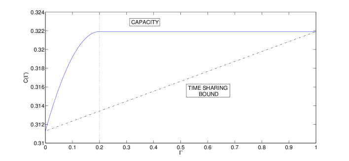
Figure 7: Cost-capacity trade off for Example 1. Time sharing is strictly sub-optimal.

Note 6 (Cut-off point $\approx 0.2$ in Fig. 7)

An observation from this example which is really surprising is that in order to achieve the maximum capacity (which is at $\Gamma=1)$ one needs to only observe a fraction of states $\approx 0.2$. This threshold however can also be theoretically derived. Essentially we find out the range of $\Gamma\in[0,1]$ for which the capacity achieving joint distribution in $C(\Gamma)$ induces exactly the same marginals, $P_{X|S}$ as when the cost is unity. Let $p^{\ast}_{1}$, $p^{\ast}_{2}$ and $p^{\ast}_{3}$ be optimal distributions for cost $\Gamma$ as in Eq. 82. The marginals are equal to

$$P(X=0|S=0)=(1-\Gamma)p^{\ast}_{1}+\Gamma p^{\ast}_{2}$$ (83)

$$P(X=0|S=1)=(1-\Gamma)p^{\ast}_{1}+\Gamma p^{\ast}_{3}.$$ (84)

For $\Gamma=1$, we can easily compute $P(X=0|S=0)=0.4$ and $P(X=0|S=1)=0.6$. Therefore for marginals to be same,

$$(1-\Gamma)p^{\ast}_{1}+\Gamma p^{\ast}_{2}=0.4$$ (85)

$$(1-\Gamma)p^{\ast}_{1}+\Gamma p^{\ast}_{3}=0.6,$$ (86)

or

$$\Gamma(p^{\ast}_{3}-p^{\ast}_{2})=0.2.$$ (87)

Since $p^{\ast}_{2},p^{\ast}_{3}\in[0,1]$, it is easy to see that if the cost $\Gamma\stackrel{{\scriptstyle>}}{{\sim}}0.2$, we can find $(p^{\ast}_{1},p^{\ast}_{2},p^{\ast}_{3})$ such that $C(\Gamma)=C(1)$. At $\Gamma=0.2$, optimal scheme is $X=S_{e}\oplus 1\mbox{ if }S_{e}\neq\ast$, and $Bern(0.5)$ otherwise.

V-A2 [Causal Probing] : To Observe or Not to Observe Channel State at Encoder , with no channel state at the Decoder.

Figure 8: Example 2

Example 2 (Binary States, $S(\alpha)$ channel and $BSC(\delta)$)

Consider the communication system shown in Fig. 8 with binary input and output with $\epsilon=0.5$, $\alpha=0.1$ and $\delta=0.3$. Here states are not known to the decoder and encoder uses partial state information causally to generate channel input symbols. Actions are binary with cost, $\Lambda(a)=a$. $A=1$ corresponds to an observation of the channel state while $A=0$ to a lack of an observation. The evaluation of capacity expression involves an auxiliary random variable. We compute its lower bound on capacity numerically using Theorem as shown in Fig. 9. Here also clearly time sharing is not optimal.

Note 7

Note the interesting phenomenon in this example too (as in Example 1), where we just need to observe roughly a fraction of state $\sim 0.5$ to obtain the capacity at unit cost. This can be reasoned in a similar manner as reasoned for Example 1.

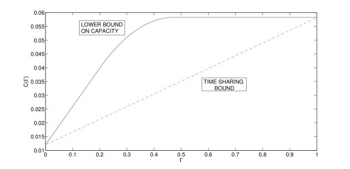
Figure 9: Cost-capacity trade off for Example 2. The dotted straight line is obtained by time sharing between zero cost and unit cost capacity (Scheme 1). Time sharing between a scheme for which $A=g(U)=U$ in Theorem 2 (call it Scheme 2) and Scheme 1 gives a lower bound on the capacity indicated by solid line. It is evident that naive Scheme 1 (time sharing scheme between extreme capacities at zero and unit cost) is strictly sub-optimal.

Example 3 (Binary States, Multiplier Channel with Power Constraints.)

Consider a multiplier channel with binary inputs, outputs and states, $Y=S\cdot X$ where $S\sim Bern(0.5)$. Again note that actions are binary with $\Lambda(a)=a$ and $A=1$ corresponds to an observation of the channel state while $A=0$ to a lack of an observation. Let

$$p_{\ast} = p(x=1|s_{e}=\ast)$$ (88)

$$p_{0} = p(x=1|s_{e}=0)$$ (89)

$$p_{1} = p(x=1|s_{e}=1).$$ (90)

We see that capacity under the power constraint,

$$p(x=1)\leq P_{0}\in[0,1],$$ (91)

is

$$C(\Gamma,P_{0}) = \max\frac{1}{2}h_{2}\left[(1-\Gamma)p_{\ast}+\Gamma p_{1}\right]$$ (93)

subject to

$$(1-\Gamma)p_{\ast}+\frac{\Gamma}{2}(p_{0}+p_{1})=P_{0}$$

For $P_{0}=0.25$, we have

$$C(\Gamma,P_{0}=0.25) = 0.5h_{2}\left[\frac{1+2\Gamma}{4}\right]\mbox{ if }\Gamma\in[0,0.5]$$ (94)

$$C(\Gamma,P_{0}=0.25) = 0.5\mbox{ if }\Gamma\in[0.5,1].$$ (95)

The plot for $P_{0}=0.25$ is shown in Fig. 10.

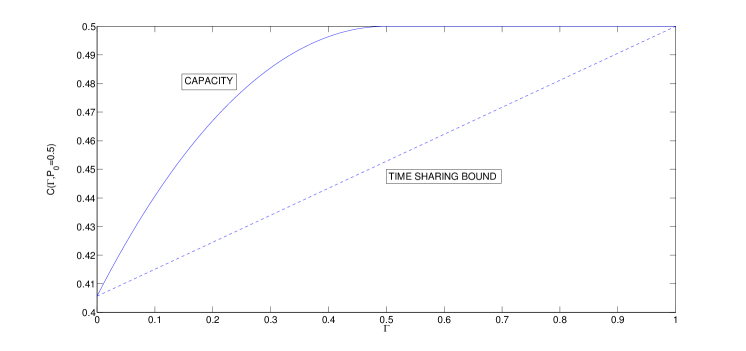
Figure 10: Cost-capacity trade off for Example 3 for $P_{0}=0.25$. The dotted straight line is obtained by time sharing between zero cost and unit cost capacity.

V-B Continuous Channels

V-B1 ‘Learning’ to Write on a Dirty Paper :

Using standard arguments, it can be shown that the capacity results carry over to the case of continuous channels with power constraints on input symbols. Let us recall the setting in Dirty Paper Coding. Costa in [17] considered the communication system as in Fig. 11.

Figure 11: Dirty Paper Coding as in [17]

The output of the channel is given as $Y^{n}=X(M,S^{n})+S^{n}+Z^{n}$, where

• Channel state or Interference $S^{n}$ is i.i.d. $S^{n}\sim\mathcal{N}(0,QI)$ independent of i.i.d. noise, $Z^{n}\sim\mathcal{N}(0,NI)$.

• Channel state or interference is known to the encoder non-causally. Encoder hence generates channel inputs $X^{n}(M,S^{n})$ which are cost constrained, i.e., $\frac{1}{n}\sum_{i=1}^{n}X_{i}^{2}\leq P$.

• Decoder has no knowledge of channel state or interference.

It was shown that the capacity of this channel is $C(P/N)=\frac{1}{2}\log_{2}(1+P/N)$ which is equal to the capacity of a standard gaussian channel with signal to noise ratio $P/N$. This is strictly larger than the capacity when $S^{n}$ is unknown to both encoder and decoder, i.e., $\frac{1}{2}\log_{2}(1+P/(Q+N))$.

We now consider the setting as in Fig. 12.

Figure 12: Learning to write on a Dirty Paper.

While in Writing on Dirty Paper, it was assumed that interference or channel state was completely available, but this might not be true in real systems one might have to pay a price to acquire this information. Hence in contrast to writing on a paper where intensity and positions of all dirt spots are known, we have to take action to learn where the paper is most dirty, hence the name Learning to Write on a Dirty Paper. Actions are binary, with cost function, $\Lambda(a)=a$. Here also $A=1$ corresponds to an observation of the channel state while $A=0$ to a lack of an observation. Also,

$$S_{e}=h(S,A) = \ast\mbox{ if }A=0$$ (96)

$$S_{e}=h(S,A) = S\mbox{ if }A=1,$$ (97)

where $\ast$ stands for erasure or no information.

Invoking Theorem 3, we have the capacity,

$$C(\Gamma,P)=\max[I(U;Y)-I(U;S_{e}|A)]=\max[I(A,U;Y)-I(U;S_{e}|A)],$$ (98)

where maximization is over joint distribution,

$$f_{A,U,S,S_{e},X,Y}=P_{A}f_{S}{\bf 1}_{\{S_{e}=h(S,A)\}}{\bf 1}_{\{X=f(U,S_{e})\}}f_{Y|X,S}$$ (99)

such that, $p(A=1)\leq\Gamma$ and $\mathsf{E}[X^{2}]\leq P$. We give a lower bound on this capacity by considering a simple power splitting achievable scheme. Let us assume $X|(A=0)\sim\mathcal{N}(0,P_{1})$ and $X|(A=1)\sim\mathcal{N}(0,P_{2})$. Clearly $C(\Gamma,P)$ is maximized when $p(A=1)=\Gamma$. Therefore we have from power constraints,

$$(1-\Gamma)P_{1}+\Gamma P_{2}\leq P.$$ (100)

Further we assume, given action $A$, channel input $X$ is independent of $U,S,Z$. Let

$$U|(A=0) = X|(A=0)$$ (101)

$$U|(A=1) = X|(A=1)+\alpha(P_{2})S,$$ (102)

where $\alpha(P_{2})=P_{2}/(P_{2}+1)$. Since $Y=X+S+Z$, we have,

$$Y|A=0\sim g_{0} = \mathcal{N}(0,P_{1}+Q+N)$$ (103)

$$Y|A=1\sim g_{1} = \mathcal{N}(0,P_{2}+Q+N)$$ (104)

$$Y\sim g = (1-\Gamma)\mathcal{N}(0,P_{1}+Q+N)+\Gamma\mathcal{N}(0,P_{2}+Q+N).$$ (105)

Considering this distribution gives the following lower bound on capacity,

$$C_{lower} = \max_{P_{1},P_{2}}[I(A,U;Y)-I(U;S_{e}|A)]$$ (106)

$$= \max_{P_{1},P_{2}}[I(A;Y)+I(U;Y|A)-I(U;S_{e}|A)]$$

$$\stackrel{{\scriptstyle(a)}}{{=}} \max_{P_{1},P_{2}}[h(g)-(1-\Gamma)h(g_{0})-\Gamma h(g_{1})+(1-\Gamma)I(X;Y|A=0)+\Gamma(I(U;Y|A=1)-I(U;S|A=1))]$$

$$\stackrel{{\scriptstyle(b)}}{{=}} \max_{P_{1},P_{2}}[h(g)-(1-\Gamma)h(g_{0})-\Gamma h(g_{1})+(1-\Gamma)C(P_{1}/(Q+N))+\Gamma C(P_{2}/N)],$$ (108)

where

• (a) follows from the fact that $S_{e}$ is just erasure for $A=0$, while for $A=1$ is equal to $S$. $h(g)$ denotes the differential entropy of a continuous random variable with distribution $g$.

• (b) follows from the fact that when $A=0$,

  $$I(X;Y|A=0) = h(Y|A=0)-h(Y|X,A=0)$$ (109)

  $$= h(\mathcal{N}(0,P_{1}+Q+N))-h(\mathcal{N}(0,Q+N)$$ (110)

  $$= \frac{1}{2}\log_{2}(1+P/(Q+N))=C(P/(Q+N)),$$ (111)

  while for $A=1$ following the similar steps as in [17][Eq. 3,4,5,6,7] we obtain,

  $$I(U;Y|A=1)-I(U;S|A=1)=\frac{1}{2}\log_{2}(1+P/N)=C(P/N).$$ (112)

  Fig. 13 shows the plot of $C_{lower}$ with $\Gamma$ for $P=Q=N=1$, which indeed performs better than naive time sharing between $C(P/N)$ and $C(P/(Q+N))$.

  

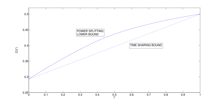
  Figure 13: Power Splitting lower bound on capacity for Learning to Write on Dirty Paper in Fig. 12.

V-B2 Fading Channels with Power Control

We revisit the setting of fading channels with encoder and decoder state information as in [11], but now the encoder takes actions to acquire the channel state from receiver state estimation, while decoder already knows the channel state. This is depicted in Fig. 14. Here $g[i]$ denotes the i.i.d. channel states which take value in a finite state, $\mathcal{S}=\{g_{1},g_{2}\}$ with equal probability. $n[i]$ is i.i.d. gaussian noise $\sim\mathcal{N}(0,N/2)$. Bandwidth for communication is $B$. $\gamma_{1}=\frac{Pg_{1}}{NB}$ and $\gamma_{2}=\frac{Pg_{2}}{NB}$ are signal to noise ratios, such that $\gamma_{1}<\frac{\gamma_{2}}{1+2\gamma_{2}}$. Actions are binary which correspond to observe or not to observe state at encoder with cost functions $\Lambda(a)=a$ and cost constraint $\Gamma$. $f$ is defined as in Theorem 1. From results in [11], we know that,

• Capacity when only decoder knows the state information

  $$C(0)=\frac{B}{2}\log_{2}(1+\gamma_{1})+\frac{B}{2}\log_{2}(1+\gamma_{2}).$$ (113)

• Capacity when encoder also knows the channel state (possibly through a noiseless feedback from decoder) in addition to decoder,

  $$C(1)=\frac{B}{2}\log_{2}(1+2\gamma_{2}).$$ (114)

The above capacities form the extreme cases of zero and unit cost respectively for the communication system in Fig. 14. Using Theorem 1, we have the capacity for the communication system in Fig. 14 with bandwidth $B$ as

$$C=\max_{P_{A}f_{X|S_{e}}}2BI(X;Y|S)=\max_{P_{A},f_{X|S_{e}}}2B[h(Y|S)-h(\mathcal{N}(0,NB))],$$ (115)

such that $\mathsf{E}[\Gamma(A)]\leq\Gamma$ and $\mathsf{E}[X^{2}]\leq P$. Clearly maximum is attained for $p(A=1)=\Gamma$. To obtain a lower bound we assume the following,

$$X|(S_{e}=\ast) \sim \mathcal{N}(0,P_{\ast})$$ (116)

$$X|(S_{e}=g_{1}) \sim \mathcal{N}(0,P_{1})$$ (117)

$$X|(S_{e}=g_{2}) \sim \mathcal{N}(0,P_{2}).$$ (118)

This implies,

$$Y|(S=g_{1}) \sim (1-\Gamma)\mathcal{N}(0,NB+P_{\ast}g_{1})+\Gamma\mathcal{N}(0,NB+P_{1}g_{1})$$ (119)

$$Y|(S=g_{1}) \sim (1-\Gamma)\mathcal{N}(0,NB+P_{\ast}g_{2})+\Gamma\mathcal{N}(0,NB+P_{2}g_{2}),$$ (120)

with power constraints,

$$\mathsf{E}[X^{2}]=(1-\Gamma)P_{\ast}+\frac{\Gamma}{2}(P_{1}+P_{2})\leq P.$$ (121)

Hence a lower bound on capacity is,

$$C_{lower}(\Gamma,P)=2B\max_{P_{\ast},P_{1},P_{2}}\left[\frac{h(f_{Y|S=g_{1}})+h(f_{Y|S=g_{2}})}{2}-h(\mathcal{N}(0,NB))\right],$$

$$\mbox{subject to }(1-\Gamma)P_{\ast}+\frac{\Gamma}{2}(P_{1}+P_{2})\leq P.$$ (122)

We plot $C_{lower}(\Gamma,P)$ as a function of $\Gamma$ for $P=N=1$, and $g_{1}=0.01,g_{2}=1$ in Fig. 15.

Figure 14: Fading channels with encoder taking actions to acquire channel state for adaptive power control.

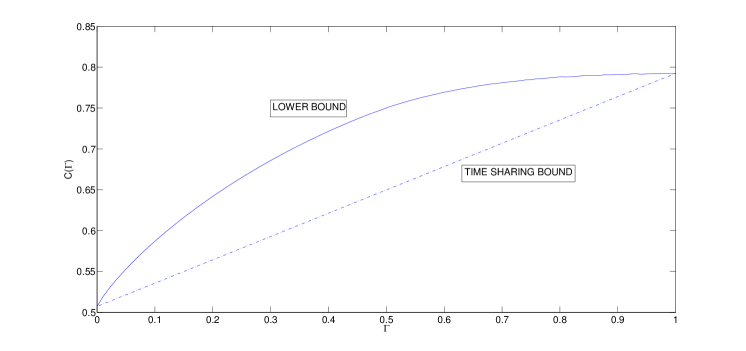
Figure 15: Lower bound on fading channel communication system in Fig. 14. Time sharing is evidently highly sub-optimal.

VI Conclusion

In this work, we obtain ‘Probing Capacity’ of systems which are characterized as follows :

• Channel is DMC with i.i.d states.

• Encoder takes costly actions and probes the channel for channel state information. This may be used causally or non-causally to generate channel input symbols.

• Decoder takes costly actions and probes the channel to obtain state information which is then used to construct message estimate.

We also worked out examples of discrete and continuous channels in cases where only encoder probed the channel for states. We not only showed that a naive time sharing scheme is strictly sub-optimal but also showed a pleasing phenomenon (see Example 1. in Section V) where one needs to observe only a fraction of states to obtain maximum rate of transmission i.e. rate when cost of state observation at encoder is not constrained.

As directions of future work, following are important questions/conjectures worth spending time and energy,

• What if encoder actions depend on past sampled state, i.e., $A_{e,i}=A_{e,i}(M,S_{e}^{i-1})$ for the case when partial state information is to be used non-causally ? Can capacity be increased ?

• What about probing capacity for channels with memory ?

• Does the Example 4 on ‘Learning to write on a dirty paper’ also support the pleasing phenomenon when we can observe only a fraction of states and still achieve Costa’s dirty paper coding capacity, $C(P/N)$ ?

• What if we take action to sample or not feedback at encoder or decoder for channels with memory ?

Some of the results concerning sampling or not the feedback for finite state channels (FSC) have been characterized in [18], while the rest are under investigation.

Appendix A Concavity of Capacity in Cost

We prove the concavity of cost constrained capacity in Theorem 4 by concavification argument. Consider ‘concavification’ of capacity in Theorem 4 as

$$C^{Q}(\Gamma)=\max[I(U;Y,S_{d}|A_{d},Q)],$$ (123)

where maximization is over all joint distributions of the form

$$P_{Q,S,A_{d},U,A_{e},S_{e},X,Y,S_{d}}(s,a_{d},u,a_{e},s_{e},x,y,s_{d})$$ (124)

$$= P_{Q}(q)P_{S}(s)P_{A_{d}|Q}(a_{d}|q)P_{U|A_{d},Q}(u|a_{d},q){\bf 1}_{\{a_{e}=g(u,a_{d},q)\}}$$

$$P_{S_{e}|S,A_{e}}(s_{e}|s,a_{e}){\bf 1}_{\{x=f(u,s_{e},a_{d},q)\}}P_{Y|X,S}P_{S_{d}|S,A_{d}}(s_{d}|s,a_{d}),$$

for some $P_{Q},P_{A_{d}|Q},P_{U|A_{d}|Q},g,f$ such that $\mathsf{E}[\Lambda(A_{e},A_{d})]\leq\Gamma$. Clearly $C^{Q}(\Gamma)\geq C(\Gamma)$. Left is to prove $C^{Q}(\Gamma)\leq C(\Gamma)$.

$$I(U;Y,S_{d}|A_{d},Q) = H(Y,S_{d}|A_{d},Q)-H(Y,S_{d}|U,A_{d},Q)$$ (125)

$$\leq H(Y,S_{d}|A_{d})-H(Y,S_{d}|U,A_{d},Q)$$ (126)

$$= I(U^{\prime};Y,S_{d}|A_{d}),$$ (127)

where last inequality follows from the defining $U^{\prime}=(U,Q)$. Proof is completed by noting that the joint distribution of $(S,A_{d},U^{\prime},A_{e},S_{e},X,Y,S_{d})$ is same as that of $(S,A_{d},U,A_{e},S_{e},X,Y,S_{d})$.

Appendix B Proof of Markov Chain $X_{i}-(S_{e,i},A_{i})-S_{i}$

Since $X_{i}=X_{i}(M,S_{e}^{n})$, it suffices to prove $(M,S_{e}^{n})-(S_{e,i},A_{i})-S_{i}$. We observe the joint distribution can be factorized as,

$$P(M,A^{n},S^{n},S^{n}_{e}) = P(M)\prod_{i=1}^{n}P(S_{i})P(A_{i}|M)P(S_{e,i}|S_{i},A_{i})$$ (128)

$$= \Phi_{1}(A^{n\backslash i},M,S_{e}^{n\backslash i},S^{n\backslash i},A_{i})\Phi_{2}(S_{i},S_{e,i},A_{i})$$ (129)

$$= \Phi^{{}^{\prime}}_{1}(A^{n\backslash i},M,S_{e}^{n},S^{n\backslash i},A_{i},S_{e,i})\Phi_{2}(S_{i},S_{e,i},A_{i})$$ (130)

which implies the Markov Chain $(A^{n\backslash i},M,S_{e}^{n},S^{n\backslash i})-(S_{e,i},A_{i})-S_{i}$, which in turn implies $(M,S_{e}^{n})-(S_{e,i},A_{i})-S_{i}$.

Appendix C Proof of Markov Chains in Theorem 4

We will prove the following markov chains,

1. $U_{i}-A_{d,i}-S_{i}$.

2. $A_{e,i}-(U_{i},A_{d,i})-S_{i}$.

3. $(S_{e,i},S_{d,i})-(S_{i},A_{e,i},A_{d,i})-U_{i}$.

4. $X_{i}-(U_{i},S_{e,i},A_{d,i})-(A_{e,i},S_{i},S_{d,i})$.

5. $Y_{i}-(X_{i},S_{i})-(U_{i},A_{d,i},A_{e,i},S_{e,i},S_{d,i})$.

MC3 and MC5 follow from the DMC assumption in problem definition. Now for the rest consider the induced probability distribution by the given encoding and decoding scheme,

$$P_{M,A_{e}^{n},S^{n},S^{n}_{e},X^{n},Y^{n},A_{d}^{n},S^{n}_{d}}(m,a_{e}^{n},s^{n},s^{n}_{e},x^{n},y^{n},a^{n}_{d},s^{n}_{d})$$ (131)

$$= \frac{1}{\mathcal{M}}{\bf 1}_{\{a_{e}^{n}=A_{e}^{n}(m)\}}\prod_{i=1}^{n}{\bf 1}_{\{a_{d,i}=A_{d,i}(y^{i-1})\}}P_{S}(s_{i})P_{S_{e},S_{d}|S,A_{e},A_{d}}(s_{e,i},s_{d,i}|s_{i},a_{e,i},a_{d,i})$$

$$\times\prod_{i=1}^{n}{\bf 1}_{\{x_{e,i}=X_{e,i}(m,s_{e}^{i})\}}P_{Y|X,S}(y_{i}|x_{i},s_{i}).$$

Averaging over $(S^{n}_{i+1},S_{e,i}^{n},X^{n}_{i},Y^{n}_{i},S_{d,i}^{n},A_{d,i+1}^{n})$, we get

$$P_{M,A_{e}^{n},S^{i},S^{i-1}_{e},X^{i-1},Y^{i-1},A_{d}^{i-1},S^{i-1}_{d}}(m,a_{e}^{n},s^{i},s^{i-1}_{e},x^{i-1},y^{i-1},a^{i-1}_{d},s^{i-1}_{d})$$ (132)

$$= P_{S}(s_{i})\times\frac{1}{\mathcal{M}}{\bf 1}_{\{a_{e}^{n}=A_{e}^{n}(m)\}}{\bf 1}_{\{a_{d,i}=A_{d,i}(y^{i-1})\}}\prod_{j=1}^{i-1}{\bf 1}_{\{a_{d,j}=A_{d,j}(y^{j-1})\}}P_{S}(s_{j})P_{S_{e},S_{d}|S,A_{e},A_{d}}(s_{e,j}s_{d,j}|s_{j},a_{e,j},a_{d,j})$$

$$\times\prod_{j=1}^{i-1}{\bf 1}_{\{x_{e,j}=X_{e,j}(m,s_{e}^{j})\}}P_{Y|X,S}(y_{j}|x_{j},s_{j}))$$

$$= \Phi_{1}(S_{i})\Phi_{2}(M,A_{e}^{n},S^{i-1},S^{i-1}_{e},X^{i-1},Y^{i-1},A_{d}^{i},S^{i-1}_{d})$$ (133)

$$= \Phi_{1}^{\prime}(S_{i},A_{d,i})\Phi_{2}(A_{d,i},U_{i},X^{i-1}).$$ (134)

Eq. (133) implies $A_{d,i}$ is independent of $S_{i}$ while Eq. (134) implies markov chain $(U_{i},X^{i-1})-A_{d,i}-S_{i}$ which in turn implies MC1. MC2 is straightforward as $U$ contains $A_{e}^{n}$.

Now averaging over $(S^{n}_{i+1},S_{e,i+1}^{n},X^{n}_{i+1},Y^{n}_{i},S_{d,i+1}^{n},A_{d,i+1}^{n})$ in Eq. (131) we obtain,

$$P_{M,A_{e}^{n},S^{i},S^{i}_{e},X^{i},Y^{i-1},A_{d}^{i-1},S^{i-1}_{d}}(m,a_{e}^{n},s^{i},s^{i}_{e},x^{i},y^{i-1},a^{i-1}_{d},s^{i-1}_{d})$$ (135)

$$= P_{S}(s_{i})P_{S_{e},S_{d}|S,A_{e},A_{d}}(s_{e,i},s_{d,i}|s_{i},a_{e,i},a_{d,i})$$

$$\times\frac{1}{\mathcal{M}}{\bf 1}_{\{a_{e}^{n}=A_{e}^{n}(m)\}}{\bf 1}_{\{x_{i}=X_{i}(m,s_{e}^{i})\}}{\bf 1}_{\{a_{d,i}=A_{d,i}(y^{i-1})\}}\prod_{j=1}^{i-1}P_{S}(s_{j})P_{S_{e},S_{d}|S,A_{e},A_{d}}(s_{e,j},s_{d,j}|s_{j},a_{e,j},a_{d,j})$$

$$\times\prod_{j=1}^{i-1}{\bf 1}_{\{x_{e,j}=X_{e,j}(m,s_{e}^{j})\}}P_{Y|X,S}(y_{j}|x_{j},s_{j}){\bf 1}_{\{a_{d,j}=A_{d,j}(y^{j-1})\}}$$

$$= \Phi_{1}(S_{i},S_{e,i},S_{d,i},A_{e,i},S_{e,i})\Phi_{2}(M,A_{e}^{n},S^{i-1},S^{i-1}_{e},X^{i},Y^{i-1},A_{d}^{i},S^{i-1}_{d})$$ (136)

$$= \Phi^{\prime}_{1}(S_{i},A_{e,i},S_{d,i},U_{i},S_{e,i},A_{d,i})\Phi^{\prime}_{2}(U_{i},S_{e,i},A_{d,i},X^{i},S^{i-1}).$$ (137)

This implies the Markov Chain, $(S^{i-1},X^{i})-(U_{i},S_{e,i},A_{d,i})-(S_{i},A_{e,i},S_{d,i})$ which implies MC4.

References

- [1] C. E. Shannon, “Channels with side information at the transmitter,” IBM J. Res. Dev., vol. 2, no. 4, pp. 289–293, 1958.
- [2] A. V. Kuznetsov and B. S. Tsybakov, “Coding in a memory with defective cells,” Probl. Contr. and Inform. Theory., vol. 10, no. 2, pp. 52–60, 1974.
- [3] S. I. Gel’fand and M. S. Pinsker, “Coding for channel with random parameters,” Problems of Control Theory, vol. 9, no. 1, pp. 19–31, 1980.
- [4] C. D. Heegard and A. A. El Gamal, “On the capacity of computer memory with defects,” IEEE Trans. Inf. Theor., vol. 29, no. 5, pp. 731–739, September 1983.
- [5] G. Keshet, Y. Steinberg, and N. Merhav, “Channel coding in the presence of side information,” Found. Trends Commun. Inf. Theory, vol. 4, no. 6, pp. 445–586, 2007.
- [6] H. H. Permuter and T. Weissman, “Source coding with a side information ’vending machine’ at the decoder,” in ISIT’09: Proceedings of the 2009 IEEE international conference on Symposium on Information Theory. Piscataway, NJ, USA: IEEE Press, 2009, pp. 1030–1034.
- [7] A. D. Wyner and J. Ziv, “The rate-distortion function for source coding with side information at the decoder,” IEEE Trans. Inform. Theory, vol. 22, pp. 1–10, 1976.
- [8] T. Weissman, “Capacity of channels with action-dependent states,” in ISIT’09: Proceedings of the 2009 IEEE international conference on Symposium on Information Theory. Piscataway, NJ, USA: IEEE Press, 2009, pp. 1794–1798.
- [9] K. Kittichokechai, T. Oechtering, M. Skoglund, and R. Thobaben, “Source and channel coding with action-dependent partially known two-sided state information,” in ISIT’10: Proceedings of the 2010 IEEE international conference on Symposium on Information Theory, June 2010, pp. 629 –633.
- [10] D. L. Donoho, “Compressed sensing,” IEEE Trans. Inform. Theory, vol. 52, pp. 1289–1306, 2006.
- [11] A. J. Goldsmith and P. P. Varaiya, “Capacity of fading channels with channel side information,” IEEE Trans. Inform. Theory, vol. 43, pp. 1986–1992, Nov. 1997.
- [12] I. Csiszar and J. Korner, Information Theory: Coding Theorems for Discrete Memoryless Systems. Orlando, FL, USA: Academic Press, Inc., 1982.
- [13] A. E. Gamal and Y. H. Kim, “Lecture notes on network information theory,” CoRR, vol. abs/1001.3404, 2010.
- [14] T. M. Cover and J. A. Thomas, Elements of information theory. New York, NY, USA: Wiley-Interscience, 1991.
- [15] M. Salehi, “Cardinality bounds on auxiliary variables in. multiple-user theory via the method of ahlswede and korner,” Department of Statistics, Stanford University, Stanford, CA, Tech. Rep. 33, August 1978.
- [16] A. Zaidi, L. Vandendorpe, and P. Duhamel, “Lower bounds on the capacity regions of the relay channel and the cooperative relay-broadcast channel with non-causal side information.” jun. 2007, pp. 6005 –6011.
- [17] M. Costa, “Writing on dirty paper (corresp.),” Information Theory, IEEE Transactions on, vol. 29, no. 3, pp. 439 – 441, may. 1983.
- [18] H. Asnani, H. H. Permuter, and T. Weissman, “To feed or not to feed back,” in preparation.