A new method for determining geometry of planetary images

Abstract

This paper presents a novel semi-automatic image processing technique to estimate accurately, and objectively, the disc parameters of a planetary body on an astronomical image. The method relies on the detection of the limb and/or the terminator of the planetary body with the VOronoi Image SEgmentation (VOISE) algorithm (Guio, P. and Achilleos, N., 2009). The resulting map of the segmentation is then used to identify the visible boundary of the planetary disc. The segments comprising this boundary are then used to perform a “best” fit to an algebraic expression for the limb and/or terminator of the body. We find that we are able to locate the centre of the planetary disc with an accuracy of a few tens of one pixel. The method thus represents a useful processing stage for auroral “imaging” based studies.

1 Introduction

During the last two decades, the Hubble Space Telescope (HST) has provided resolved images of both Jupiter and Saturn in the ultraviolet (UV) spectral region. Such images capture with high sensitivity and high resolution, the spectacular auroral phenomena occurring in the polar regions of the gas giants as a result of energetic magnetospheric particles raining down onto the planet’s upper atmosphere. Auroral images have become a particularly useful diagnostic tool for morphological characterisations of the aurora and its boundaries. This is a crucial prerequisite for identifying the aurora’s physical origin (e.g. Prangé et al., 1996, 1998; Grodent et al., 2003b, a; Clarke et al., 2005; Badman et al., 2008; Lamy et al., 2009).

Imaging is also complementary to in situ measurements of the plasma environment provided, e.g.  by the Cassini spacecraft, currently orbiting Saturn. Combining remote imaging with in situ data allows the study of magnetospheric processes and how they affect the planet’s upper atmosphere, and ionosphere via the planet’s magnetic field (Dougherty et al., 1998; Clarke et al., 2002; Bunce et al., 2008; Talboys et al., 2009), and the footprint auroral emission of satellites (Clarke et al., 2002; Bonfond et al., 2007; Wannawichian et al., 2008). Such studies require accurate projection of the geographic and geomagnetic coordinate systems of the planet onto the plane of the two-dimensional image. Auroral dynamics can be studied using time series of images. For these purposes, the location of the planet centre needs to be known accurately. Unfortunately, HST pointing parameters are not generally known with sufficient accuracy for such applications. The precision of the guide star catalogue together with the uncertainty in the start time of the tracking motion is on the order of [1]$\mathrm{arc\,sec}$ while it is desired to have an accuracy of the order of [1]pixel, i.e. [0.02–0.03]$\mathrm{arc\,sec}$ for the Space Telescope imaging spectrograph (STIS) and Advanced Camera for Surveys (ACS) instruments, in order to to locate any structure accurately or to build polar projections of the auroral emissions.

In addition, ground-based observations with telescopes such as the NASA Infrared Telescope Facility (IRTF) and United Kingdom Infra-Red Telescope (UKIRT), both located at Mauna Kea, Hawaii, have provided images of Jupiter and Saturn with resolved auroral structures in the infrared (IR) waveband. IR images and spectra also allow the study of the dynamics and morphology of the H_3^+ molecular ion, a principal component of giant ionospheres (Miller et al., 2006). Again, the location of the planet centre needs to be known accurately to make use of these images, but for similar reasons as the HST case, the pointing parameters are not known with sufficient accuracy for the images from IRTF and UKIRT telescopes. The resolution of the IRTF imaging facility and the UKIRT imager-spectrometer (UIST) are respectively of the order of [0.04]$\mathrm{arc\,sec}$ pixel^-1 and [0.12]$\mathrm{arc\,sec}$ pixel^-1 or better.

The problem of the location of the planet on auroral images has been addressed by various authors and studies (e.g. Bonfond et al., 2007; Nichols et al., 2008; Bonfond et al., 2009) but to our knowledge no published work provides any detailed description of the method used. Here we propose a novel semi-automatic method to estimate accurately and objectively the position, size and orientation of a planetary body. The method consists of three phases: (i) detection of the limb of the planet disc using our image segmentation algorithm VOronoi Image SEgmentation (VOISE) (see Guio, P. and Achilleos, N. (2009) for details), (ii) selection of points (Voronoi seeds) from the VOISE map that surround the limb, and (iii) nonlinear fit (Levenberg-Marquardt algorithm) of the selected set of data from VOISE to a disc model. Phase (i) is performed once while phases (ii) and (iii) can be repeated in order to improve the accuracy.

In section 2, we give analytic expressions for the projection of the limb and the terminator in the sky-plane. In section 3, the method is developed. In section 4 we illustrate our method on IR images of Jupiter collected with the IRTF and UKIRT telescopes. We discuss the performance of our method and summarise our conclusions in section 5.

2 Limb and terminator equations

A planet’s pressure surface can be modelled by an ellipsoid, more precisely an oblate spheroid, with equatorial radius (semi-major axis) $r_{e}$ and polar radius (semi-minor axis) $r_{p}$, where $r_{p}^{2}=r_{e}^{2}(1{-}e^{2})$, and $e$ is the eccentricity of the spheroid. The parameters are readily available, for instance, from the NASA Navigation and Ancillary Information Facility SPICE system (Acton, 1996).

Figure 1: Sketch of the geometry of the planet and the observer. The eccentricity of the planetary ellipsoid is exaggerated for clarity.

The planet rotation vector is assumed to be along the $z$-axis with positive angular velocity $\vec{\omega}$ as shown in Fig. 1. Without loss of generality, we can further assume that the observer is located in the $(x,z)$-plane, i.e. setting the longitude of the observer ${\lambda_{\oplus}}{=}0$, and the observing direction as the vector ${\vec{\delta}_{\oplus}}=(\cos{\beta_{\oplus}},0,\sin{\beta_{\oplus}})$ where ${\beta_{\oplus}}$ is the planetocentric latitude (sub-Earth latitude), the (negative) angle between the $x$-axis and ${\vec{\delta}_{\oplus}}$ in Fig. 1. The limb of the planet consists of the points on the planet surface where the local normal ${\hat{\vec{n}}_{S}}$ is perpendicular to the observing direction ${\vec{\delta}_{\oplus}}$, i.e. ${\hat{\vec{n}}_{S}}\cdot{\vec{\delta}_{\oplus}}=0$. The entire limb is contained in a single plane and is an ellipse, and the normal vector to the plane containing the limb ${\hat{\vec{n}}_{L}}$ has coordinates $(\cos{\beta_{{\hat{\vec{n}}_{L}}}},0,\sin{\beta_{{\hat{\vec{n}}_{L}}}})$ where

$$\cos{\beta_{{\hat{\vec{n}}_{L}}}} =\frac{(1{-}e^{2})\cos{\beta_{\oplus}}}{\sqrt{(1{-}e^{2})^{2}\cos^{2}{\beta_{\oplus}}+\sin^{2}{\beta_{\oplus}}}}$$ (1)

$$\sin{\beta_{{\hat{\vec{n}}_{L}}}} =\frac{\sin{\beta_{\oplus}}}{\sqrt{(1{-}e^{2})^{2}\cos^{2}{\beta_{\oplus}}+\sin^{2}{\beta_{\oplus}}}}$$ (2)

The ellipse of the limb can then be projected onto the plane of the sky $(x_{s},y_{s})$, i.e. on a plane perpendicular to the observing direction ${\vec{\delta}_{\oplus}}$ (see Fig. 1). The projection of the limb in the sky-plane is also an ellipse with the following algebraic equation in the sky plane coordinate system

$$\frac{x_{s}^{2}}{r_{e}^{2}}+\frac{y_{s}^{2}}{r_{e}^{2}(1{-}e^{2}\cos^{2}{\beta_{\oplus}})} =1.$$ (3)

where the $y_{s}$-axis is chosen to lie in the $(x,z)$-plane. It can be seen from Eq. (3) that the limb always appears with a semi-major axis equal to the equatorial radius of the planet and a semi-minor axis between the polar radius of the planet (in the case of an equatorial view ${\beta_{\oplus}}=0$) and the equatorial radius of the planet (in the case of a polar view ${\beta_{\oplus}}=\pm\pi/2$). Equivalently the eccentricity of the ellipse formed by the limb in the sky is $e_{L}=e\cos{\beta_{\oplus}}$.

The terminator (boundary between day and night side) can be visualised as the limb for the direction corresponding to the location of the Sun ${\vec{\delta}_{\odot}}$ (i.e. such that the local normal ${\hat{\vec{n}}_{T}}$ is perpendicular to ${\vec{\delta}_{\odot}}$) but projected onto the sky plane along the observing direction ${\vec{\delta}_{\oplus}}$, i.e. directed towards Earth. The Sun direction is defined by its planetocentric latitude ${\beta_{\odot}}$ (sub-solar latitude) and its relative longitude (solar phase angle) to the observing direction $\Delta\lambda={\lambda_{\odot}}{-}{\lambda_{\oplus}}$. In the coordinate system $(x^{\prime},y^{\prime},z^{\prime})$ where $z^{\prime}$ is also aligned to the rotation axis of the planet but the plane $(x^{\prime},z^{\prime})$ has been rotated about the planet rotation axis to contain the Sun direction, the vector ${\hat{\vec{n}}_{T}}$ has coordinates $(\cos{\beta_{{\hat{\vec{n}}_{T}}}},0,\sin{\beta_{{\hat{\vec{n}}_{T}}}})$ where

$$\cos{\beta_{{\hat{\vec{n}}_{T}}}} =\frac{(1{-}e^{2})\cos{\beta_{\odot}}}{\sqrt{(1{-}e^{2})^{2}\cos^{2}{\beta_{\odot}}+\sin^{2}{\beta_{\odot}}}},$$ (4)

$$\sin{\beta_{{\hat{\vec{n}}_{T}}}} =\frac{\sin{\beta_{\odot}}}{\sqrt{(1{-}e^{2})^{2}\cos^{2}{\beta_{\odot}}+\sin^{2}{\beta_{\odot}}}}$$ (5)

In the situation where ${\vec{\delta}_{\oplus}}\times{\hat{\vec{n}}_{T}}=\vec{0}$, the limb and the terminator are coincident. Otherwise the vector ${\vec{\delta}_{\oplus}}\times{\hat{\vec{n}}_{T}}$ is contained in the sky plane (since it is perpendicular to ${\vec{\delta}_{\oplus}}$) and in the plane of the terminator. Therefore the projections onto the sky-plane of the limb and the terminator intersect at two points called the cusps, and the line joining the two cusps has direction ${\vec{\delta}_{\oplus}}\times{\hat{\vec{n}}_{T}}$.

The two cusp points define the major axis of the ellipse formed by the sky projection of the terminator. This shape is a tilted ellipse with tilt angle $\theta_{T}$ with respect to the $x_{s}$-axis given by

$$\theta_{T}=\\ \tan^{-1}\left(\frac{(1{-}e^{2})\cos{\beta_{\odot}}\sin\Delta\lambda}{(1{-}e^{2})\cos{\beta_{\odot}}\cos\Delta\lambda\sin{\beta_{\oplus}}{-}\sin{\beta_{\odot}}\cos{\beta_{\oplus}}}\right).$$ (6)

The semi-major and semi-minor axes of the projection of the full terminator (i.e. its visible and invisible parts) onto the sky-plane are

$$a_{T}^{2} =(u^{2}{+}v^{2})t_{1}^{2}$$ (7)

$$b_{T}^{2} =(u^{2}{+}v^{2})t_{2}^{2}.$$ (8)

where the vector $\vec{u}=(u,v)$ lies in the direction defined by ${\vec{\delta}_{\oplus}}{\times}{\hat{\vec{n}}_{T}}$,

$$u =(1{-}e^{2})\cos{\beta_{\odot}}\cos\Delta\lambda\sin{\beta_{\oplus}}-\sin{\beta_{\odot}}\cos{\beta_{\oplus}},$$ (9)

$$v =(1{-}e^{2})\cos{\beta_{\odot}}\sin\Delta\lambda,$$ (10)

and $t_{1}$ and $t_{2}$ are scalars analytically derivable from $u$ and $v$

$$t_{1}^{2} =\frac{r_{e}^{2}(1{-}e^{2}\cos^{2}{\beta_{\oplus}})}{u^{2}(1{-}e^{2}\cos^{2}{\beta_{\oplus}})+v^{2}},$$ (11)

$$t_{2}^{2} =\frac{r_{e}^{2}(1{-}e_{\beta_{\odot}}^{2})(ad{-}bc)^{2}}{(dv{+}bu)^{2}(1{-}e_{\beta_{\odot}}^{2})+(cv{+}au)^{2}}$$ (12)

where $e_{\beta_{\odot}}$ is the eccentricity of the ellipse formed by the terminator in its own plane and can be expressed as function of the Sun planetocentric latitude ${\beta_{\odot}}$ and the eccentricity of the spheroid $e$

$$e_{\beta_{\odot}}^{2} =e^{2}\left(1-\frac{\sin^{2}{\beta_{\odot}}}{1-e^{2}\cos^{2}{\beta_{\odot}}}\right),$$ (13)

and where

$$a =\cos\Delta\lambda,$$ (14)

$$b =-\sin{\beta_{{\hat{\vec{n}}_{T}}}}\sin\Delta\lambda,$$ (15)

$$c =\sin\Delta\lambda\sin{\beta_{\oplus}},$$ (16)

$$d =\sin{\beta_{{\hat{\vec{n}}_{T}}}}\cos\Delta\lambda\sin{\beta_{\oplus}}{+}\cos{\beta_{{\hat{\vec{n}}_{T}}}}\cos{\beta_{\oplus}}$$ (17)

Finally the signed distance (as measured along ${\hat{\vec{n}}_{T}}$) between a point $(x_{T},y_{T})$ of the projection of the terminator onto the sky-plane, and the plane of the terminator itself is given by

$$D_{T}=(\cos{\beta_{{\hat{\vec{n}}_{T}}}}\sin\Delta\lambda)x_{T}+\\ ({-}\cos{\beta_{{\hat{\vec{n}}_{T}}}}\cos\Delta\lambda\sin{\beta_{\oplus}}{+}\sin{\beta_{{\hat{\vec{n}}_{T}}}}\cos{\beta_{\oplus}})y_{T},$$ (18)

and points with $D_{T}{>}0$ belong to the visible terminator (from the Earth observer’s point of view) while points with $D_{T}{<}0$ are hidden, and the case $D_{T}{=}0$ corresponds to cusp points. Similarly the signed distance (measured along ${\vec{\delta}_{\odot}}$) between a point of the limb’s projection onto the sky-plane $(x_{L},y_{L})$, and the plane perpendicular to the direction of the Sun ${\vec{\delta}_{\odot}}$ is given by

$$D_{L}=(\cos{\vec{\delta}_{\odot}}\sin\Delta\lambda)x_{L}+\\ \left({-}\cos{\vec{\delta}_{\odot}}\cos\Delta\lambda\sin{\beta_{\oplus}}{+}\sin{\vec{\delta}_{\odot}}\frac{\cos{\beta_{\oplus}}}{1{-}e^{2}}\right)y_{L},$$ (19)

and points such that $D_{L}{>}0$ belong to the illuminated limb while points such that $D_{L}{<}0$ are in the shade, and the case $D_{L}{=}0$ corresponds to cusp points.

3 Planetary disc extraction method

As pointed out the proposed method to extract the orientation and shape of the planetary disc from an image consists of three phases, described in the following sections.

3.1 Phase (i) VOISE image reduction

The first stage consists of partitioning the image into regions, i.e. simplify and/or change the representation of an image into something that is more physically meaningful and easier to analyse. VOISE is a dynamic algorithm for partitioning the underlying pixel grid of an image into regions according to a prescribed homogeneity criterion (Guio, P. and Achilleos, N., 2009). A VOISE segmentation returns a map of the image in the form of a Voronoi diagram (VD) where each Voronoi region (VR) is a polygon, within which the data are homogeneous with respect to prescribed criteria. When running the VOISE segmentation algorithm on an image of a planetary object we expect that the transition region between the illuminated planet and the sky (i.e. the limb or the terminator) consists of a ring of relatively small Voronoi polygons, indicating that at this region, the intensity is changing very quickly over small spatial scales. In this representation we can classify the “ring” of tiny Voronoi polygons surrounding the larger central polygons as a cluster in itself that can be used for fitting a terminator and/or a limb. The map generated at the end of the VOISE division phase provides the largest number of seeds and smallest Voronoi polygons (see Guio, P. and Achilleos, N. (2009) for more detail).

3.2 Phase (ii) points selection

The selection of seeds from the computed VOISE map requires “crude” estimates for the planet centre $(x_{c},y_{c})$, the equatorial radius (semi-major axis) $r_{e}$, the polar radius (semi-minor axis) $r_{p}$ and the tilt angle $\alpha$. The seeds from the segmentation are considered part of the neighbourhood of the limb and/or terminator if they lie inside a prescribed elliptic torus. A point belongs to the torus if its coordinates $(x,y)$ fulfil the following inequalities

$$\varepsilon_{m}^{2}\leq\frac{{x^{\prime}}^{2}}{a^{2}}+\frac{{y^{\prime}}^{2}}{b^{2}}\leq\varepsilon_{M}^{2},$$ (20)

where $\varepsilon_{m}$ and $\varepsilon_{M}$ (with $\varepsilon_{m}<1<\varepsilon_{M}$) represent the inner and outer ellipses of the torus, and where $(x^{\prime},y^{\prime})$ are obtained from $(x,y)$ by translation with ${-}(x_{c},y_{c})$ followed by rotation with ${-}\alpha$, i.e.

$$\begin{bmatrix}x^{\prime}\\ y^{\prime}\end{bmatrix}=\begin{bmatrix}\cos\alpha&\sin\alpha\\ {-}\sin\alpha&\cos\alpha\end{bmatrix}\begin{bmatrix}x{-}x_{c}\\ y{-}y_{c}\end{bmatrix}.$$ (21)

As well as satisfying the condition given by Eqs. (20–21), the polygons used in the fitting procedure must also have a surface area smaller than a prescribed value (equivalently a “length scale” $\mathcal{L}$ smaller than a maximum prescribed value $\mathcal{L}_{M}$). The maximum length scale $\mathcal{L}_{M}$ has to be larger than the minimum distance between seeds $d_{m}$ that is set for the VOISE division phase.

It is also possible to filter out “bands” of polar angle in order to remove those regions with auroral emission clearly outside the planetary limb as illustrated in section 4.

3.3 Phase (iii) fitting of points

Fitting of quadrics (such as circles and ellipses) to a given set of points in the plane is a problem that arises in many application areas, e.g. computer graphics, pattern recognition, coordinate meteorology. Many algorithms minimise a quantity in some least-square sense. Such fitting algorithms for quadrics can be separated into categories of “best fit” (“geometric fit”) and “algebraic fit” (Gander et al., 1994; Fitzgibbon et al., 1999). In addition the clustering technique is another technique to fit an ellipse, such as methods based on the Hough transform (Yuen et al., 1989).

In the “best fit”, the quantity to minimise is the geometric distance between the fitted curve and the given set of points. In this case, curves may be represented in parametric form, which is well suited for minimising the sum of the squares of the distances.

In the “algebraic fit” the curve is represented algebraically, i.e. in the plane by an equation of the form $F(x,y)=0$. If a point is on the curve, then its coordinates $(x,y)$ are a zero of the function $F$ and represent an algebraic distance. These methods are usually equivalent to solving a linear system of equations subject to some constraint on the quadric coefficients (Bookstein, 1979; Taubin, 1991; Fitzgibbon et al., 1999). The constraint may be such that the optimal solution is computed directly, and no iterations are needed. The disadvantage of the “algebraic fit” is that we are uncertain what we are minimising in a geometrical sense and in many cases those constraints lead to fits which are not invariant under Euclidean transformations such as translations and rotations, i.e. different coordinate systems produce different fitted curves. Another limitation is that these methods can fit only one primitive (or shape) at a time, therefore the data should be segmented into a set of basic shapes before fitting each shape independently. Nonetheless the algebraic solution is useful as an initial guess for the geometrical fit.

We have developed a “best fit” tool based on the the Levenberg-Marquardt method (Marquardt, 1963), for solving nonlinear least-square problems. This method performs a minimisation of the sum of the squares of the weighted distances between the $m$ selected seeds $\vec{s}_{i}$ ($i{=}1\ldots m$) from the Voronoi map, and the “best”-fitting curve with parametric representation $(x,y)=\vec{f}(\phi;\vec{p})$ (Bard, 1974; Gander et al., 1994). The minimisation consists in adjusting iteratively the set of curve parameters $\{\phi_{i}\}$ (that locate the “best” points on the curve), together with the vector of global parameters $\vec{p}$ (that describe the global shape of the curve). Mathematically the function to minimise is written

$$Q(\phi_{1},\phi_{2},\ldots,\phi_{m},\vec{p})=\sum_{i=1}^{m}\frac{\left\|\vec{s}_{i}-\vec{f}(\phi_{i};\vec{p})\right\|^{2}}{\sigma_{i}^{2}}.$$ (22)

The parametric representation $\vec{f}$ for a circle and an ellipse are given by Eq. (23) and Eq. (24) respectively. $\sigma_{i}^{2}$ represents the variance of the location of a given seed. An estimate for this uncertainty can be readily computed as the mean distance from the seed to all the points within the VR. Alternatively a length scale $\mathcal{L}_{i}$ of the polygon can be inferred from the square root of its surface area (Guio, P. and Achilleos, N., 2009), and can be thought of as the “average” section length through the polygon in all directions. Thus considering the disc with same surface area $\mathcal{A}$ as the polygon, the variance in distance of the disc points from its centre is given by $\sigma^{2}=\mathcal{A}/(2\pi)=\mathcal{L}^{2}/2$ (where surface area is used as the weighting factor for variance). This expression can thus be used as a reasonable approximation for the variance of the location of the seeds.

The Levenberg-Marquardt method is optimised to switch continuously from a method which quickly approaches the minimum (the steepest descent method), when far from the minimum, to a more precise but slower method (the Newton method), when approaching the minimum.

Finally we note that a priori knowledge about any of the parameters can be used to constrain the fitting, otherwise an appropriate number of free parameters may be simultaneously determined from the fitting procedure.

3.3.1 Fitting a circle

The parametric form used for the circle is given by

$$\vec{f}(\phi;[x_{c},y_{c},r])=\begin{bmatrix}x_{c}\\ y_{c}\end{bmatrix}{+}r\begin{bmatrix}\cos\phi\\ \sin\phi\end{bmatrix}.$$ (23)

where $x_{c}$, $y_{c}$ and $r$ are respectively the coordinates of the centre and the radius of the circle. Note that the values of $\phi$ for each data point $\vec{s}_{i}$ are updated along with the global parameters $\vec{p}=[x_{c},y_{c},r]$ at each iteration. The parameter $\phi$ represents the polar angle, measured from the $x$-axis, of the line joining the centre $(x_{c},y_{c})$ of the circle to the point on the circle which is associated with the relevant data point.

3.3.2 Fitting an ellipse

The parametric form used for the ellipse is given by

$$\vec{f}(\phi;[x_{c},y_{c},a,b,\alpha])=\\ \begin{bmatrix}x_{c}\\ y_{c}\end{bmatrix}{+}\begin{bmatrix}\cos\alpha&{-}\sin\alpha\\ \sin\alpha&\cos\alpha\end{bmatrix}\begin{bmatrix}a\cos\phi\\ b\sin\phi\end{bmatrix}$$ (24)

where $x_{c}$, $y_{c}$, $a$, $b$ and $\alpha$ are respectively the coordinates of the centre, the semi-major axis, semi-minor axis and the tilt angle of the ellipse (angle measured from the $x$-axis to the semi-major axis). In this case the parameter $\phi$ does not represent the polar angle, measured from the $x$-axis, of the line joining the centre $(x_{c},y_{c})$ of the ellipse to the point on the ellipse. The parameter $\phi$ is sometimes referred to as eccentric anomaly and is related to the polar angle $\theta$ by the following equation:

$$b\tan\phi=a\tan(\theta{-}\alpha).$$ (25)

3.3.3 Fitting the limb and the terminator

Note that the the limb and terminator can be represented in a single parametric form $[x_{LT}(\phi),y_{LT}(\phi)]=\vec{f}_{LT}(\phi)$ using the equations given in section 2. This shape can be fitted by considering the three following transformations: homothetic transformation with scale factor $c$, rotation with angle $\alpha$ and translation by $(x_{c},y_{c})$

$$\vec{f}(\phi;[x_{c},y_{c},c,\alpha])=\\ \begin{bmatrix}x_{c}\\ y_{c}\end{bmatrix}{+}c\begin{bmatrix}\cos\alpha&{-}\sin\alpha\\ \sin\alpha&\cos\alpha\end{bmatrix}\begin{bmatrix}x_{LT}(\phi)\\ y_{LT}(\phi)\end{bmatrix}$$ (26)

In this case the global parameters for $\vec{f}_{LT}(\phi)$ are the geometric parameters ${\beta_{\oplus}}$, ${\beta_{\odot}}$, $\Delta\lambda$, $r_{e}$, $r_{p}$ introduced in section 2 (as well as the distance from the observer to the planet to convert projected length into pixels units). These parameters may be determined by e.g. SPICE. The unknown global parameters to optimise for $\vec{f}(\phi)$ are the planet centre $(x_{c},y_{c})$, the scale factor $c$ and tilt angle $\alpha$.

3.4 Algorithm

Phase (i) is performed once while phases (ii) and (iii) can be iterated. The iteration process improves the selection of seeds for the fit and removes any “outliers” that might be included using the crude estimates for the parameters, therefore improving the accuracy of the fit. The tolerance on fractional improvement of $Q$ defined in Eq. (22) is set to $10^{-3}$. Such tolerance ensures convergence of the Levenberg-Marquardt algorithm in a few iterations leading to an accuracy of the estimate of the centre coordinates and the radii of the order of one pixel or better.

4 Application to planetary images

4.1 Ellipse for complete planet

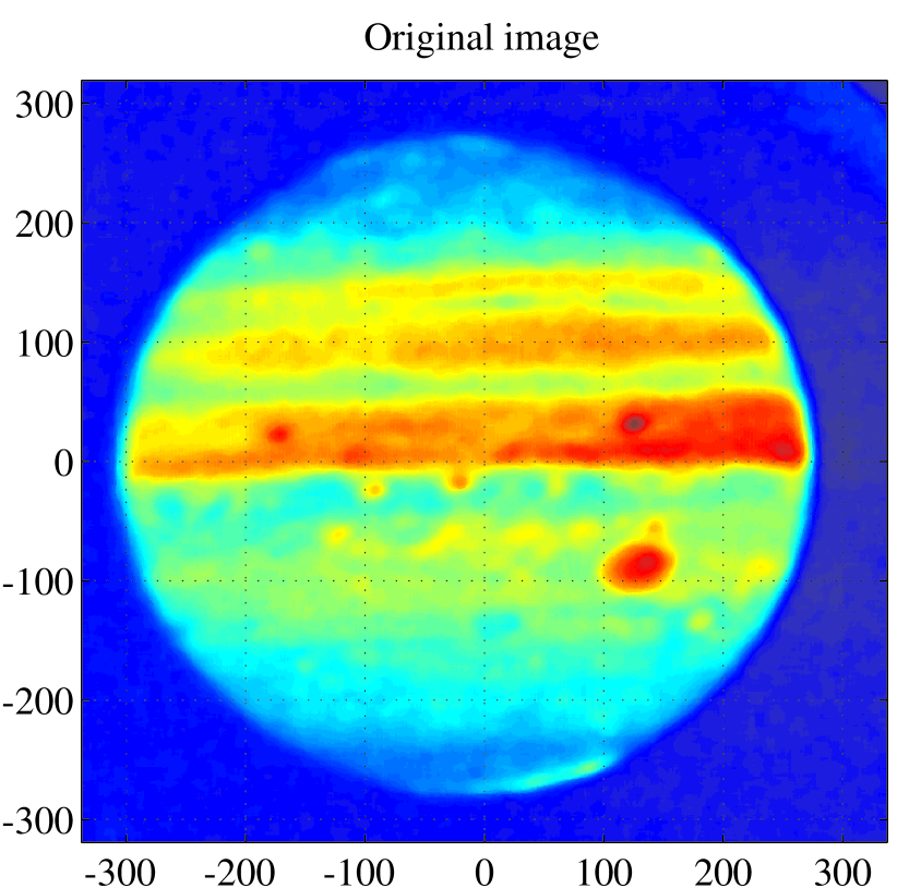
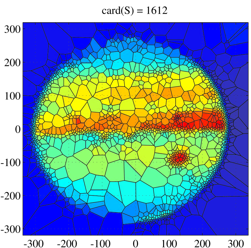
Figure 2: In the upper panel, median-filtered IR image collected by UKIRT (in arbitrary intensity unit) and in the lower panel the resulting Voronoi tessellation from the VOISE algorithm. The [1612]tiles of the tessellation are uniformly coloured using the median intensity of the pixels that are lying within each polygon. The axes are labelled in pixels unit and the point with coordinates $(0,0)$ is the centre of the image. The colour code for both images is shown in Fig. 4.

The image presented here (see upper panel of Fig. 2) to illustrate the location method of a complete planetary disc has been obtained using the [3.8]m UKIRT at Mauna Kea observatory, Hawaii, with the near-IR UIST guide camera (Ramsay Howat et al., 2004). This image has not been flux calibrated but the sky background noise has been subtracted, and the intensities are thus in arbitrary units.

UIST is a [1–5]μm imager-spectrometer with a [1024×1024]pixels InSb array. In imaging mode there are two plate scales available, with resolution [0.12]$\mathrm{arc\,sec}$/pixel and [0.06]$\mathrm{arc\,sec}$ pixel^-1, giving fields of view of [2×2]$\mathrm{arc\,min}$^2 and [1×1]$\mathrm{arc\,min}$^2 respectively.

UIST was used to observe Jupiter at a resolution of [0.12]$\mathrm{arc\,sec}$ pixel^-1, with the Brackett alpha filter ([50]per cent cut-on at [4.024]μm and [50]per cent cut-off at [4.078]μm) in exposures of [10]s. The Brackett line is an IR emission line of the H atom. Thus this emission should contribute many of the photons as well as H_3^+. In this part of the IR spectrum, the emission of the giant planets is dominated by several lines of H_3^+, and the spectral measurement of individual lines allows determination of H_3^+ temperatures and column densities of the planet (Miller et al., 2006). The UIST camera was used in conjunction with the dual-beam polarimeter module IRPOL2 for spectropolarimetry measurements under an observation campaign of Jupiter on August 4, 2008.

Fig. 2 illustrates phase (i) of detection of the limb using VOISE on an image collected by UKIRT at [10:13:00]UT. The size of the image is [679×639]pixels and it has been pre-processed by a nonlinear filter —a median filter— of size [11×11]pixels in order to lower noise in the image (Gonzalez & Woods, 2007). Whenever such noise filter is used as pre-processing to the VOISE segmentation, the size of the mask should be chosen to be larger than the minimum seed distance $d_{m}$ to be of any effect. The main idea of this filter is to slide a window with specified size and replace each centre pixel of the window by the median of the pixels lying in the window. The VOISE parameters (Guio, P. and Achilleos, N., 2009) are (i) division phase: $d^{2}_{m}=\unit[9]{pixels^{2}}$, $p_{\mathrm{D}}=\unit[97]{percent}$ (ii) merging phase: $p_{\mathrm{M}}=\unit[50]{percent}$, $\Delta\mu=\unit[20]{percent}$ and $\Delta\mathcal{H}=\unit[30]{percent}$ (iii) two iterations in the regularisation phase. The resulting segmentation contains [1612]polygons (lower panel in Fig. 2). Note the compactness of the polygons in regions with small length scales along the limb and near the equator.

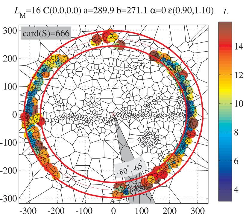
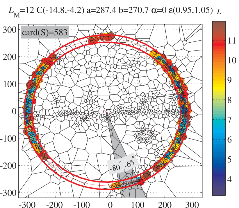
Figure 3: Selection of the seeds from the VOISE tessellation for two iterations of the phases (ii) and (iii). During the first iteration (upper plot) $\unit[666]{seeds}$ are selected as neighbours of the limb while for the second iteration the numbers of seeds considered for the fit is reduced to [583]seeds. The size of each coloured marker is proportional to the surface area of the selected polygon. The limits of the torus are shown in thick red lines while the nominal ellipse is shown as a thin red line and the red cross is the centre of the torus.

Table 1: Parameters of the fitted ellipse resulting from two iterations of phases (ii) and (iii). The ellipses are shown in Fig. 4. Note that the tilt angle has not been fitted and has been fixed to $\alpha=0$. # iter is the number of iterations performed in order to converge with the prescribed tolerance and the normalised $\chi^{2}$ provides an indication of the goodness of the fit. The “guess”, “fit 1” and “fit 2” ellipses are shown in Fig. 4.

$x_{c}$ $y_{c}$ $a$ $b$ $\alpha$ # iter $\chi^{2}$ guess $0.0$ $0.0$ $289.9$ $271.1$ $0$ fit 1 $-14.8{\pm}0.4$ $-4.2{\pm}0.7$ $287.4{\pm}0.4$ $270.7{\pm}1.2$ $0$ $3$ $4.10$ fit 2 $-15.5{\pm}0.3$ $-3.5{\pm}0.7$ $287.6{\pm}0.4$ $272.2{\pm}1.1$ $0$ $3$

Figure 4: Initial guess for the ellipse and the ellipses resulting from the two successive fits for the original image shown in Fig. 2. The points selected for each fit are as shown in Fig. 3.

Fig. 3 illustrates phase (ii) of selecting the set of points from the segmentation to be used as the neighbourhood of the planetary limb. The upper panel shows the first iteration, using crude estimates of the ellipse parameters to define the large torus with $\varepsilon_{m}=0.9$ and $\varepsilon_{M}=1.1$, and a relatively large scale length parameter $\mathcal{L}_{M}=\unit[16]{pixels}$. The lower panel shows the selection process for the second iteration with parameters provided by the result of the first fit. The torus has been re-centred and its thickness reduced by setting $\varepsilon_{m}=0.9$ and $\varepsilon_{M}=1.05$. The scale length parameter has also been reduced to $\mathcal{L}_{M}=\unit[12]{pixels}$ (to be compared to $d_{m}=\unit[3]{pixels}$). In both iterations, seeds in the neighbourhood of the faint emission outside the limb near the South pole have been rejected whenever the polar angle of the seed $\varphi$ with respect to the centre $C(x_{c},y_{c})$ is in the range $\unit[-80]{{}^{\circ}}{<}\varphi{<}\unit[-65]{{}^{\circ}}$, i.e. the seed lies inside the grey shaded sector depicted in Fig. 3.

Fig. 4 illustrates phase (iii) consisting of the nonlinear fitting of the selected points (shown in Fig. 3) to an ellipse in parametric form given by Eq. (24). The planetary disc modelled as a single ellipse is justified in the situation where the disc is nearly fully illuminated, as is the case here. The curve labelled “guess” corresponds to crude estimates of the ellipse parameters, i.e. the coordinates of the planet centre correspond to the centre of the image and the equatorial and polar radii are derived using SPICE. The curve “fit1” is the curve with parameters after first fit, i.e. with the seeds as seen in the upper panel of Fig. 3 and the the curve labelled “fit2” corresponds to seeds as seen in the lower panel of Fig. 3.

The parameters, error estimates and fitting parameters are given in Table 4.1. It is interesting to note that the estimated parameters related to the $x$-direction ($x_{c}$ and $a$) have smaller errors compared to the parameters relates to the $y$-direction ($y_{c}$ and $b$) which is a consequence of the large sampling of seeds around the equator. We have also checked, for consistency, that the curve parameters $\{\phi_{i}\}$ and the global parameters $\vec{p}$ together with their errors $\{\Delta\phi_{i}\}$ and $\Delta\vec{p}$ provide error in positioning of the points consistent with the values used for the weights $\sigma_{i}$ in Eq. (22).

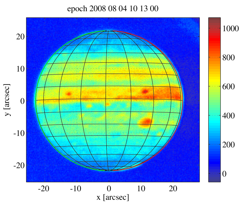
Figure 5: Image scaled in $\mathrm{arc\,sec}$ and the projection in the sky-plane of a latitude-longitude grid of Jupiter computed using data from SPICE and the fitted parameters of Jupiter’s disc.

Fig. 5 presents the image with a (planetocentric) latitude-longitude grid (with [10]^∘ step in latitude and [20]^∘ in longitude) computed using the coordinates of the centre of Jupiter’s disc obtained from the nonlinear fitting and the projection geometry computed using SPICE. The Central Meridian Longitude (CML) of Jupiter at the time of the observation is [157.5]deg. The limb is shown on the right side of the planet (red solid line) while the terminator is shown on the left side (green solid line). The parameters are ${\beta_{\oplus}}=\unit[-1.5]{{}^{\circ}}$, ${\beta_{\odot}}=\unit[-1.4]{{}^{\circ}}$ and $\Delta\lambda=\unit[5.3]{{}^{\circ}}$. The equatorial radius for the final fit is $r_{e}=\unit[70958]{km}$ with an eccentricity $e=0.32$ while the values provided by SPICE are $r_{e}=\unit[71492]{km}$ and $e=0.35$. The illuminated limb in the considered near-IR waveband is thus slightly smaller than Jupiter’s [1]Bar pressure surface as given by SPICE.

4.2 Circle for partial planet

Figure 6: In the top panel, IRTF image processed by a median filter followed by histogram equalisation (in arbitrary intensity unit). In the lower panel the result of the segmentation by VOISE. The colour code for the [494]tiles is the same as for the segmentation presented in the lower panel in Fig. 2. The axes are labelled in pixels unit and coordinates $(0,0)$ correspond to the centre of the planet provided by the original Image Reduction and Analysis Facility (IRAF) data reduction, taking into account an estimate based on the telescope pointing (Satoh & Connerney, 1999). The colour code for both images is shown in Fig. 8.

The image presented in this section (upper panel in Fig. 4.1) has been chosen to illustrate the case with partial occlusion of the planetary disc. It was collected with NASA’s [3.8]m IRTF at Mauna Kea observatory, Hawaii using the imaging facility (Shure et al., 1994) at wavelength [3.43]μm (a wavelength sensitive to H_3+). The image was collected during a campaign on June 28, 1995 at [11:14:52]UT. This image has not been flux calibrated but the sky background noise has been subtracted, and the intensities are thus in arbitrary units.

The NSFCAM is a [1–5]μm imager with a [256×256]pixels InSb detector. Three different magnifications are available: [0.3]$\mathrm{arc\,sec}$ pixel^-1, [0.15]$\mathrm{arc\,sec}$ pixel^-1 and [0.06]$\mathrm{arc\,sec}$ pixel^-1 corresponding to a field of view of [76.8]$\mathrm{arc\,sec}$, [37.9]$\mathrm{arc\,sec}$ and [14.1]$\mathrm{arc\,sec}$ respectively. The NSFCam has been upgraded (NSFCam 2) with a [2048×2048]pixels Hawaii-2RG detector. The image scale will be [0.04]$\mathrm{arc\,sec}$ pixel^-1 with field of view [80×80]$\mathrm{arc\,sec}$^2.

Fig. 4.1 shows the results of phase (i) of the method using VOISE on an image collected by UKIRT at [0721]UT. The image has size [256×256]pixels. Note that the image has been pre-processed by a median filter of size [7×7]pixels to lower noise level, followed by a histogram equalisation (Gonzalez & Woods, 2007). The histogram equalisation is performed in order to increase the global contrast of the original image (which is shown in Fig. 9). It consists of a nonlinear adjustment of the intensities in order to better distribute the image intensity histogram and accomplishes this by effectively “spreading out” the most frequent intensity values. Alternatively, the contrast in the low intensity range can also be enhanced by taking the logarithm of the ratio of the image pixels relative to the estimated noise level, if available. Note that we haven’t pre-processed the UKIRT image for the first example as the limb boundary was already substantially more intense than the background. The VOISE parameters have been set to (i) division phase: $d^{2}_{m}=\unit[4]{pixels^{2}}$, $p_{\mathrm{D}}=\unit[98]{percent}$ (ii) merging phase: $p_{\mathrm{M}}=\unit[50]{percent}$, $\Delta\mu=\unit[20]{percent}$ and $\Delta\mathcal{H}=\unit[30]{percent}$ (iii) two iterations in the regularisation phase.

Figure 7: Seeds selection for two iterations of phase (ii). For details see Fig. 3.

Fig. 4.1 illustrates phase (ii) of selecting the set of points from the Voronoi map to be used as within the limb neighbourhood. Note that the points with polar angle $\varphi$ with respect to the centre estimate $C(x_{c},y_{c})$ such that $\unit[-115]{{}^{\circ}}{<}\varphi{<}\unit[-65]{{}^{\circ}}$ (inside the grey shaded sector in Fig. 4.1) are filtered out to avoid bias from the seeds corresponding to the the emission outside the limb which has been highlighted by the histogram equalisation.

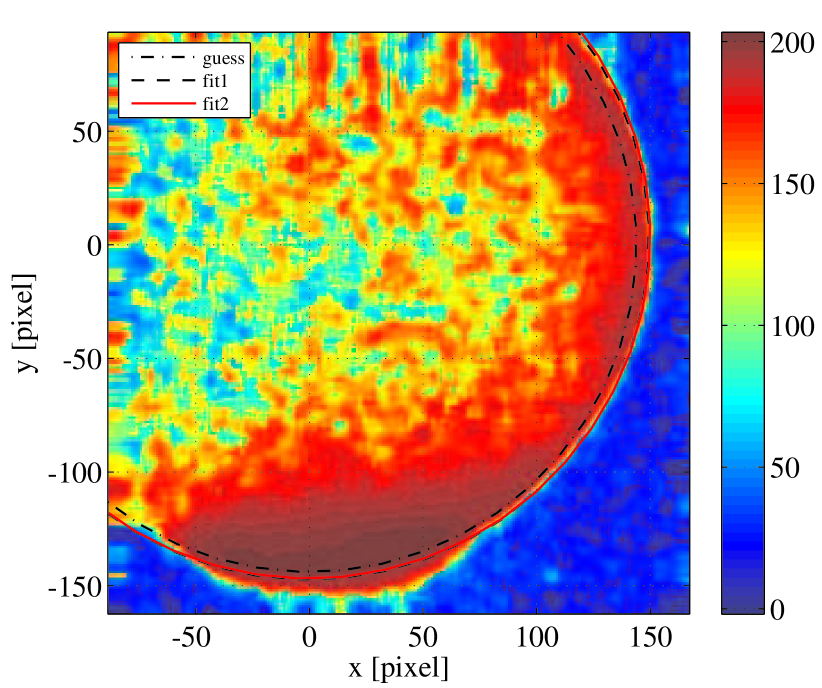
Figure 8: Initial guess for the circle and the circles “fit 1” and “fit 2” resulting from two iterations of the phases (ii) and (iii). The selected points for each iteration are shown in Fig. 4.1.

Fig. 8 illustrates phase (iii) consisting of the nonlinear fitting of the selected points (shown in Fig. 4.1) to a circle in parametric form Eq. (23). The global parameters of the circle fitted together with estimates for the error are given in Table 4.1. The circle as a model for the disc is justified in situations where only a portion of the planetary disc is in the field of view, as it is the case in the present image. Note also that in this case the distribution of the seeds is uniform from the equator to the South pole and therefore the estimated parameters related to the $x$-direction have similar errors as those related to the $y$-direction.

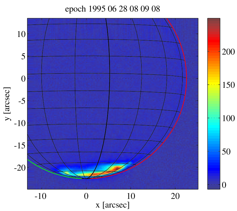
Figure 9: Original image scaled in $\mathrm{arc\,sec}$ together with the sky-plane projection of a latitude-longitude grid computed using data from SPICE and the fitted parameters of Jupiter’s disc, i.e. the circle parameters.

Table 2: Resulting parameters for the circle during the two iterations of fit. The number of iterations and the resulting normalised $\chi^{2}$ are also given. The corresponding “guess”, “fit 1” and “fit 2” circles are shown in Fig. 8.

$x_{c}$ $y_{c}$ $R$ # iter $\chi^{2}$ guess $0.0$ $0.0$ $143.9$ fit 1 $-0.3{\pm}0.9$ $2.5{\pm}0.9$ $149.8{\pm}0.9$ $3$ $2.87$ fit 2 $-0.3{\pm}0.8$ $3.5{\pm}0.8$ $150.3{\pm}0.8$ $3$

Fig. 9 presents the image with the same (planetocentric) latitude-longitude grid resolution as in Fig. 5 calculated with the coordinates of the centre and radius of Jupiter’s disc obtained from the nonlinear fitting, and the projection geometry from SPICE. The CML of Jupiter at the time of the observation is [13.5]deg. The limb and terminator are shown as red and green solid lines respectively, and the thick black line is the noon-meridian. The parameters provided by SPICE are ${\beta_{\oplus}}=\unit[-2.9]{{}^{\circ}}$, ${\beta_{\odot}}=\unit[-2.8]{{}^{\circ}}$ and $\Delta\lambda=\unit[5.3]{{}^{\circ}}$. The radius for the final fit (“fit 2”) is $r_{e}=\unit[72466]{km}$. The illuminated limb in this waveband is slightly larger than Jupiter’s [1]bar pressure surface. We also tried to fit an ellipse and it leads to a similar estimate for the centre coordinates but with larger error bars due to the increased degrees of freedom.

5 Discussion

We have presented a novel semi-automatic method to estimate accurately, and objectively, the disc parameters in an image of an illuminated planetary disc. The method is based on the “best” fit of a set of points selected from a segmentation map generated by VOISE to a curve described in a parametric form.

The segmentation phase can be improved by pre-processing the image using different techniques such as noise filtering and contrast adjustment.

Basic shapes to describe the boundary of a planetary disc include the circle and the ellipse. We also provide analytic expressions for the projection in the sky-plane of the limb and terminator of a planet modelled as ellipsoid. These expressions can easily be used to describe both limb and terminator as single curve in parametric form.

Note that the VOISE algorithm generates “intermediate” tessellations, one at the end of the division phase and one at the end of the merging phase. It is worth noting that fitting an ellipse gives the best result (smallest $\chi^{2}$) for the regularised tessellation (i.e. after merging), but errors in the fitted parameters are smaller when considering the map at the end of the division phase. The largest $\chi^{2}$ is obtained for the map generated at the end of the merging phase. This confirms that the tessellation obtained after division is optimum for our purposes. The reason for this is that VOISE merging generates more regular polygons, but very slightly degrades the position information from the division phase.

We have shown that our novel objective method to locate the planetary disc on images provides improved estimates of the centre position (as compared to the guide star catalogue) as well as the altitude when the disc is illuminated for the corresponding observational waveband.

We also showed that the use of histogram equalisation enhances the auroral emission outside the limb and therefore allows a better and unbiased estimate of the limb by allowing removal of points from this auroral emission region.

The software implementing this method is written in Matlab^® and can be made available by request to the authors.

Acknowledgements

We would like to thank M. Lystrup who kindly provided the UKIRT images.

The United Kingdom Infrared Telescope is operated by the Joint Astronomy Centre on behalf of the Science and Technology Facilities Council of the U.K.

We also like to thank J.E.P. Connerney and T. Satoh for making the IRTF data available.

This work uses data acquired at the NASA IRTF, which is operated by the University of Hawaii under Cooperative Agreement no. NNX-08AE38A with the National Aeronautics and Space Administration, Science Mission Directorate, Planetary Astronomy Program.

References

- Acton (1996) Acton C. H., 1996, Planet. Space Sci., 44, 65
- Badman et al. (2008) Badman S. V., Cowley S. W. H., Lamy L., Cecconi B., Zarka P., 2008, Ann. Geophysicæ, 26, 3641
- Bard (1974) Bard Y., 1974, Non linear parameter estimation. Academic Press, New York, iSBN 0-12-078250-2
- Bonfond et al. (2007) Bonfond B., Gérard J.-C., Grodent D., Saur J., 2007, Geophys. Res. Lett., 34, 6201
- Bonfond et al. (2009) Bonfond B., Grodent D., Gérard J., Radioti A., Dols V., Delamere P. A., Clarke J. T., 2009, J. Geophys. Res., 114, 7224
- Bookstein (1979) Bookstein F. L., 1979, Comput. Graph. Image Process., 9, 56
- Bunce et al. (2008) Bunce E. J., Arridge C. S., Clarke J. T., Coates A. J., Cowley S. W. H., Dougherty M. K., Gérard J., Grodent D., Hansen K. C., Nichols J. D., Southwood D. J., Talboys D. L., 2008, J. Geophys. Res., 113, 9209
- Clarke et al. (2002) Clarke J. T., Ajello J., Ballester G., Ben Jaffel L., Connerney J., Gérard J.-C., Gladstone G. R., Grodent D., Pryor W., Trauger J., Waite J. H., 2002, Nature, 415, 997
- Clarke et al. (2005) Clarke J. T., Gérard J., Grodent D., Wannawichian S., Gustin J., Connerney J., Crary F., Dougherty M., Kurth W., Cowley S. W. H., Bunce E. J., Hill T., Kim J., 2005, Nature, 433, 717
- Dougherty et al. (1998) Dougherty M. K., Dunlop M. W., Prange R., Rego D., 1998, Planet. Space Sci., 46, 531
- Fitzgibbon et al. (1999) Fitzgibbon A., Pilu M., Fisher R., 1999, IEEE Trans. Pattern Anal. Mach. Intell., 21, 476
- Gander et al. (1994) Gander W., Golub G. H., Strebel R., 1994, BIT Num. Math., 34, 558
- Gonzalez & Woods (2007) Gonzalez R. C., Woods R. E., 2007, Digital image processing, 3rd edn. Prenctice Hall, Upper Saddle River, NJ, iSBN 0240515749
- Grodent et al. (2003a) Grodent D., Clarke J. T., Kim J., Waite J. H., Cowley S. W. H., 2003a, J. Geophys. Res., 108, 1389
- Grodent et al. (2003b) Grodent D., Clarke J. T., Waite J. H., Cowley S. W. H., Gérard J.-C., Kim J., 2003b, J. Geophys. Res., 108, 1366
- Guio, P. and Achilleos, N. (2009) Guio, P. and Achilleos, N., 2009, Mon. Not. R. Astron. Soc., 1051
- Lamy et al. (2009) Lamy L., Cecconi B., Prangé R., Zarka P., Nichols J. D., Clarke J. T., 2009, J. Geophys. Res., 114, 10212
- Marquardt (1963) Marquardt D. W., 1963, SIAM J. Appl. Math., 11, 431
- Miller et al. (2006) Miller S., Stallard T., Smith C., Millward G., Mellin H., Lystrup M., Aylward A., 2006, Phil. Trans. Roy. Soc. London A, 364, 3121
- Nichols et al. (2008) Nichols J. D., Clarke J. T., Cowley S. W. H., Duval J., Farmer A. J., Gérard J.-C., Grodent D., Wannawichian S., 2008, J. Geophys. Res., 113, 11205
- Prangé et al. (1998) Prangé R., Rego D., Pallier L., Connerney J., Zarka P., Queinnec J., 1998, J. Geophys. Res., 103, 20195
- Prangé et al. (1996) Prangé R., Rego D., Southwood D., Zarka P., Miller S., Ip W., 1996, Nature, 379, 323
- Ramsay Howat et al. (2004) Ramsay Howat S. K., Todd S., Leggett S., Davis C., Strachan M., Borrowman A., Ellis M., Elliot J., Gostick D., Kackley R., Rippa M., 2004, in Presented at the Society of Photo-Optical Instrumentation Engineers (SPIE) Conference, Vol. 5492, Society of Photo-Optical Instrumentation Engineers (SPIE) Conference Series, A. F. M. Moorwood & M. Iye, ed., pp. 1160–1171
- Satoh & Connerney (1999) Satoh T., Connerney J. E. P., 1999, Icarus, 141, 236
- Shure et al. (1994) Shure M. A., Toomey D. W., Rayner J. T., Onaka P. M., Denault A. J., 1994, in Society of Photo-Optical Instrumentation Engineers (SPIE) Conference Series, Vol. 2198, Society of Photo-Optical Instrumentation Engineers (SPIE) Conference Series, D. L. Crawford & E. R. Craine, ed., pp. 614–622
- Talboys et al. (2009) Talboys D. L., Arridge C. S., Bunce E. J., Coates A. J., Cowley S. W. H., Dougherty M. K., 2009, J. Geophys. Res., 114, 6220
- Taubin (1991) Taubin G., 1991, IEEE Trans. Pattern Anal. Mach. Intell., 13, 1115
- Wannawichian et al. (2008) Wannawichian S., Clarke J. T., Pontius D. H., 2008, J. Geophys. Res., 113, 7217
- Yuen et al. (1989) Yuen H. K., Illingworth J., Kittler J., 1989, Image Vis. Comput., 7, 31