Magnetic field amplification and electron acceleration to near-energy equipartition with ions by a mildly relativistic quasi-parallel plasma protoshock.

Abstract

Context. The prompt emissions of gamma-ray bursts (GRBs) are seeded by radiating ultrarelativistic electrons. Kinetic energy dominated internal shocks propagating through a jet launched by a stellar implosion, are expected to dually amplify the magnetic field and accelerate electrons.

Aims. We explore the effects of density asymmetry and of a quasi-parallel magnetic field on the collision of two plasma clouds.

Methods. A two-dimensional relativistic particle-in-cell (PIC) simulation models the collision with 0.9c of two plasma clouds, in the presence of a quasi-parallel magnetic field. The cloud density ratio is 10. The densities of ions and electrons and the temperature of 131 keV are equal in each cloud, and the mass ratio is 250. The peak Lorentz factor of the electrons is determined, along with the orientation and the strength of the magnetic field at the cloud collision boundary.

Results. The magnetic field component orthogonal to the initial plasma flow direction is amplified to values that exceed those expected from the shock compression by over an order of magnitude. The forming shock is quasi-perpendicular due to this amplification, caused by a current sheet which develops in response to the differing deflection of the upstream electrons and ions incident on the magnetised shock transition layer. The electron deflection implies a charge separation of the upstream electrons and ions; the resulting electric field drags the electrons through the magnetic field, whereupon they acquire a relativistic mass comparable to that of the ions. We demonstrate how a magnetic field structure resembling the cross section of a flux tube grows self-consistently in the current sheet of the shock transition layer. Plasma filamentation develops behind the shock front, as well as signatures of orthogonal magnetic field striping, indicative of the filamentation instability. These magnetic fields convect away from the shock boundary and their energy density exceeds by far the thermal pressure of the plasma. Localized magnetic bubbles form.

Conclusions. Energy equipartition between the ion, electron and magnetic energy is obtained at the shock transition layer. The electronic radiation can provide a seed photon population that can be energized by secondary processes (e.g. inverse Compton).

1 Introduction

1.1 Observations and Context

Gamma ray bursts (GRBs) are eruptions of electromagnetic radiation at cosmological distances. One group of GRBs, those with a long duration, is attributed to the implosion of supermassive stars. This is supported by observations, where GRBs precede supernovae (Hjorth et al. 2003) and of particularly violent stellar explosions that show some resemblances with GRBs (Kulkarni et al. 1998). GRBs are thought to be signatures of plasma ejection from a forming compact object, such as a neutron star or a black hole.

The fireball model due to Meszaros & Rees (1992) and Rees & Meszaros (1994) assumes that the plasma is ejected in form of a highly relativistic collimated jet by extreme supernovae (hypernovae) and that the jet dynamics is kinematically driven. It has been used to explain the anisotropic radiation bursts. In this model, plasma clouds collide due to the nonuniform flow speed and density of the jet, which is a consequence of the nonstationarity of the jet source. The clouds can collide within the jet with Lorentz factors of a few and the cloud densities can probably vary by about an order of magnitude. The resulting internal shocks move with Lorentz factors of a few through the jet. They are thought to be responsible for the observed prompt phase of GRBs (Piran 1999; Fox & Mészáros 2006). The prompt emissions due to the jet thermalization precede the longlasting afterglow, which has its origin in the interaction of the jet plasma with the ambient medium.

The underlying mechanisms causing the observed electromagnetic radiation are still not fully understood. Highly polarized gamma-ray emission suggests the presence of an ordered magnetic field in the emitting zone (Steele et al. 2009). These primordial magnetic fields, which can be amplified further by the internal shocks, together with ultrarelativistic electrons give rise to electromagnetic emissions. The resulting photon seed can be upscattered to higher energies by secondary processes (Kirk & Reville 2010). It is not yet clear if, and to what extent, stable and large-scale magnetic fields are generated or amplified by instabilities close to internal shocks (Medvedev & Loeb 1999; Brainerd 2000; Waxman 2006). The presence of ultrarelativistic electrons in the jet also cannot be taken for granted. The dominant blackbody radiation component of GRB jets suggests a plasma temperature of $\sim$100 keV (Ryde 2005). The majority of jet electrons are thus only moderately relativistic. The energetic electrons responsible for the nonthermal radiation component of the prompt emissions (Ryde 2005) must consequently be accelerated within the jet, probably by the internal shocks.

The likely involvement of plasma collisions for both magnetic field generation/amplification and for electron acceleration and the possible presence of a guiding magnetic field, motivates our simulation study of the early stages of plasma cloud collision and shock formation.

1.2 General Plasma behaviour

The single-fluid magnetohydrodynamic (MHD) approximation can be used to model the ejection of relativistic jets by compact objects and to examine their time evolution (Nishikawa et al. 2005). However, it can not adequately describe the plasma dynamics within the shock transition layer, in which the ultrarelativistic electrons and the strong magnetic fields are generated. Many different wave-modes (e.g. upper hybrid waves, whistler waves and Bernstein mode waves) and instabilities (Bret 2009) not captured by a MHD model are present and they interplay. The wave and instability spectrum depends critically on multiple parameters of the bulk plasma, among others the electric and magnetic field orientation and strength, the plasma composition, the pre- and post shock density ratio and the temperature. In order to model the acceleration of particles, the generation of magnetic fields by internal shocks in GRB jets and their small scale structure, it is necessary to use a kinetic particle-in-cell (PIC) simulation code.

1.3 Modelling and PIC simulations

The theory of collisionless magnetised shocks divides naturally into shocks with a quasi-parallel magnetic field (treated in this work) and those with a quasi-perpendicular shock. Quasi-perpendicular shocks have been well studied in the past and in the context of SNR or Solar system shocks using both analytical and numerical approaches. Single-fluid analytical models have been unable to describe successfully the TeV emission from SNRs but hybrid or PIC simulations may provide better insight (Kirk & Dendy 2001). Nonrelativistic numerical models of perpendicular and parallel electrostatic shocks have been devised using hybrid methods, for example by (Leroy et al. 1981; Quest 1988). Perpendicular shocks have been modelled by Lee et al. (2004); Scholer & Matsukiyo (2004); Amano & Hoshino (2007); Umeda et al. (2009); Lembège et al. (2009) and many more authors with PIC simulations, while Sorasio et al. (2006) addressed fast unmagnetized shocks. Oblique, strongly magnetised shocks have been studied by Lembège & Dawson (1989); Bessho & Ohsawa (1999); Dieckmann et al. (2008); Sironi & Spitkovsky (2009); Shikii & Toida (2010); Murphy et al. (2010a).

Considerable work has been done modelling interpenetrating and colliding plasma streams in the context of GRB jets, with their attendant wave modes and instabilities. Frederiksen et al. (2004) studied using 3D PIC simulations two initially unmagnetized plasma clouds colliding with a density ratio of 3, both composed of electrons and ions. The Lorentz factor of the collision speed was 2-3. Computational constraints demanded a reduced ion-to-electron mass ratio of 16. The effects of a guiding magnetic field have been considered by Nishikawa et al. (2003); Hededal & Nishikawa (2005); Dieckmann et al. (2006) with 2D and 3D PIC simulations.

GRB jets may carry with them a significant fraction of positrons (Piran 1999). Kazimura et al. (1998); Jaroschek et al. (2004); Spitkovsky (2008) modelled with 2D and 3D PIC simulations the collision of two unmagnetized clouds, each consisting of electrons and positrons. Hoshino et al. (1992) introduced heavier ions in 1D simulations. Magnetic field effects on such collisions were taken into account by Spitkovsky (2005); Sironi & Spitkovsky (2009). Interpenetrating leptonic plasmas have been investigated by Silva et al. (2003).

The simulation results typically show the generation of magnetic fields by a filamentation of the plasma that implies a separation of the currents, provided that the guiding magnetic field is not too strong and that the flow speeds are relativistic (Cary et al. 1981). The energy density of the magnetic field reaches typically about 10% of the leptonic flow energy. However, most simulation studies could not observe a suprathermal population, as long as the plasma cloud collision speeds or the beam speeds are mildly relativistic. Such an acceleration of electrons on short spatiotemporal scales is conditional on both the presence of ions in the plasma flow and a mechanism that can transfer a significant fraction of the ion flow energy to the electrons.

Initial conditions that result in a substantial magnetic field amplification and in the electron acceleration to ultrarelativistic energies have been proposed by Bessho & Ohsawa (1999), who studied in one spatial dimension the collision of magnetized plasmas at the speed 0.9c and with a magnetic field direction tilted by 45 degrees relative to the flow velocity vector. An ion-to-electron mass ratio of 100 was used. The acceleration of electrons up to Lorentz factors of $\sim$130 has been found.

Here we consider the collision of two plasma clouds with a density ratio of 10, with a speed of 0.9c, and in the presence of a strong magnetic field. The initial magnetic field would correspond to a primordial jet magnetic field (Lyutikov et al. 2003; Granot 2003). These initial conditions are similar to those used by Bessho & Ohsawa (1999). Our magnetic field direction is, however, tilted at 0.1 radians relative to the flow direction and, most importantly, the two-dimensional simulation permits a more complex array of physical processes at a higher mass ratio. A 1D study using almost the same parameters (Dieckmann et al. 2008) suggests that the magnetic and electron energy density will increase drastically in the forming shock transition layer. This expectation is confirmed here, but we will demonstrate that the actual plasma dynamics in our 2D simulation differs notably from that in the previous 1D studies.

We demonstrate that the coherency of the circularly polarized electromagnetic wave ahead of the shock is reduced compared to what was assumed for the 1D simulations, which can be partially attributed to the failure of the guiding magnetic field to suppress the filamentation. The shock planarity, which is enforced by a 1D simulation, is destroyed here by the development of a flux tube. This flux tube is the focus of the research letter Murphy et al. (2010b), hereafter MDD. Here we examine in more detail this flux tube and the plasma conditions in the PIC simulation that result in its growth.

In this paper we perform a numerical simulation of two plasma clouds colliding, using conditions that are probably appropriate for GRBs. In Section 2 we describe the method used, in Section 3 we present some results and finally in Section 4 we discuss the results obtained.

2 The Numerical Experiments

The particle-in-cell (PIC) simulation method has been described in detail elsewhere (Dawson 1983). The plasma is represented by an ensemble of computational particles (CPs). These CPs correspond to phase space blocks rather than physical particles. Consequently, the charge $q_{i}$ and the mass $m_{i}$ of a CP of the species $i$ do not have to correspond to the equivalent of the physical particles it represents. However, the charge to mass ratio $q_{i}/m_{i}$ must equal that of the physical particle. Then the ensemble properties of all CPs representing the species $i$ are an approximation to the ensemble properties of the corresponding plasma species, e.g. an electron species or an ion species.

PIC codes approximate the Klimontovich-Dupree equations (Dupree 1963), which correspond to the solution of the Vlasov-Maxwell equations by the method of characteristics. PIC codes can capture all kinetic wave modes and instabilities found in collisionless plasma, if the simulation box size and the resolution, as well as the statistical plasma representation, are adequate.

We consider the collision of a dense plasma cloud with a tenuous one. The electrons with mass $m_{e}$ and the ions with mass $m_{i}=250m_{e}$ of the dense cloud are the species 1 and 2, respectively. The electrons of the tenuous cloud are species 3 and species 4 denotes the ions of the tenuous cloud. We normalise our variables with the plasma frequency of the species 2, with the density $n_{2}$, the charge $q_{2}$ and the mass $m_{2}$. The normalization is useful, in that it renders the simulation results independent of the plasma density, which is unknown for GRB jets. The skin depth of species 2 is $\lambda_{2}=c/\omega_{p2}$. The elementary charge is $e$. The quantities in SI units (subscript $p$) can be obtained by the substitutions $\mathbf{E}_{p}=\omega_{p2}cm_{i}\mathbf{E}/e$, $\mathbf{B}_{p}=\omega_{p2}m_{i}\mathbf{B}/e$, $\rho_{p}=en_{2}\rho$, $\mathbf{J}_{p}=ecn_{2}\mathbf{J}$, $\mathbf{x}_{p}=\lambda_{2}\mathbf{x}$ and $t_{p}=t/\omega_{p2}$. The solved equations are

$$\nabla\times\mathbf{E}=-\partial_{t}\mathbf{B},\,\nabla\times\mathbf{B}=\partial_{t}\mathbf{E}+\mathbf{J},$$ (1)

$$\nabla\cdot\mathbf{B}=0,\nabla\cdot\mathbf{E}=\rho,$$ (2)

$$d_{t}\mathbf{p}_{j}=q_{j}\left(\mathbf{E}+\mathbf{v}_{j}\times\mathbf{B}\right),\,\mathbf{p}_{j}=m_{j}\Gamma\mathbf{v}_{j},\,d_{t}\mathbf{x}_{j}=\mathbf{v}_{j}.$$ (3)

Here the subscript $j$ refers to the $j^{th}$ CP with the mass $m_{j}$ and the charge $q_{j}$. We use the Plasma Simulation Code PSC for our simulations, which is a relativistic 3d MPI parallel domain decomposed PIC code. It has been extensively used in the laser plasma community (Roth et al. 2001; Cowan et al. 2004).

2.1 Simulation Initial Conditions

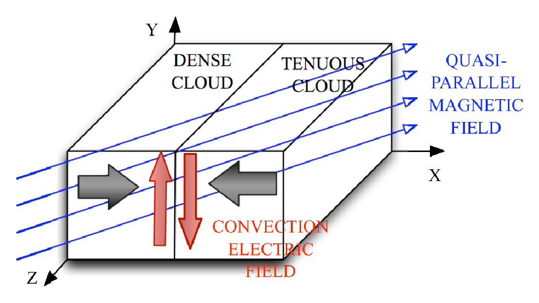
Figure 1: Sketch of simulation initial conditions

We begin the simulation with two colliding plasma clouds. Figure 1 illustrates the flow and field geometry. The inclination angle relative to the flow velocity vector of the initial magnetic field $\mathbf{B}_{0}$ is 0.1 radians and its magnitude $|\mathbf{B}_{0}|=R^{1/2}$ in our normalization, where $R=m_{i}/m_{e}=250$ is the reduced ion/electron mass ratio. The magnitude $|\mathbf{B}_{0}|$ is thus such, that the electron cyclotron frequency equals the electron plasma frequency of the dense plasma cloud. Both beams (high and low density) travel initially at $0.63c$ but in opposite directions, giving a relative speed of $0.9c$. This speed jump will be distributed over the forward and reverse shocks. The temperature of all species is $T=131$keV. The thermal velocity of the electrons is $v_{th,e}=\sqrt{kT/m_{e}}=0.83v_{b}=0.52c$. The thermal velocity is such that it is not greatly smaller than the collision speed, as expected to be for internal shocks in GRB jets. The thermal velocity of the ions is $v_{th,i}=v_{th,e}/{\sqrt{R}}=0.033c$. The initial distribution of the particles is a relativistic Maxwellian or Maxwell-Jüttner distribution. The initial density ratio is chosen to be 10. We cannot use here the piston method of Forslund & Shonk (1970). In this piston method, the plasma is reflected at a conducting wall. The plasma symmetry across the wall is exploited and only one cloud has to be modelled. This cloud is reflected onto itself by the wall and a shock develops at the collision boundary. It is a computationally efficient method. However, only a limited number of field geometries should be modeled with it. The electric fields at a conducting wall must point along the surface normal and the magnetic field orthogonal to it. We can also model with it unmagnetized plasma as in Forslund & Shonk (1970). It is furthermore not possible to let an oblique magnetic field stream with the plasma into the simulation box through an open boundary and let the electromagnetic field distribution at the conducting wall develop self-consistently when the plasma reaches it. The oblique geometry implies a flow-aligned magnetic field component, which would have to end at the front of the inflowing plasma cloud. A magnetic monopole would be the consequence. While the particular choice of the boundary condition may not affect the long term evolution of the shock far from the boundary, a representation of both colliding plasma clouds will be more realistic. In our case study, we collide two plasma clouds with different densities and, in fact, this asymmetry rules out the piston method altogether due to an absent mirror symmetry at the wall. This is physically motivated by the expectation that plasma clouds of similar but unequal density will collide in the GRB jet, although we have to point out that the collision boundary is unlikely to be as abrupt as the computationally convenient one, which we implement here. However, we do not expect a strong dependence of the key simulation results on the boundary shape. The smooth boundary used by Bessho & Ohsawa (1999) and the sharp one used by Dieckmann et al. (2008) did not result in qualitatively different simulation results. The simulation will furthermore show that the important structures form well after the initial time, when the boundary has been smeared out. The transport of the magnetic field $\mathbf{B}$ at velocity $\mathbf{u}\parallel\mathbf{x}$ gives a convection electric field $\mathbf{E}_{c}=\mathbf{u}\times\mathbf{B}$ (Baumjohann & Treumann 1996). It changes its direction at the cloud collision boundary.

2.2 Linear instability

The original motivation to pick the high initial plasma temperature, the strong guiding magnetic field $\mathbf{B}_{0}$ and the asymmetric beam density has been to suppress the filamentation instability and, thus, to enforce a planar shock (Dieckmann et al. 2008). We can test this assumption by computing the approximate linear dispersion relation under the following assumptions. An early time is considered, when both clouds overlap in a small interval along $x$. The interval is large enough to ensure that the electrons of both clouds have mixed and form a single, spatially uniform and hot distribution. The interval is small enough so that firstly the ion distribution is unchanged and secondly the magnetic field component orthogonal to the beam velocity vector has not yet been compressed to a significant amplitude. Then we can approximate the plasma in the cloud overlap layer by two counter-propagating ion beams, which move through a hot electron background along a guiding magnetic field with an amplitude that equals $250^{1/2}$. The relative speed between both ion beams is 0.9c and their density ratio is 10.

Figure 2 displays the linear dispersion relation calculated for the ion-to-electron mass ratio of $R=250$ in the simulation.

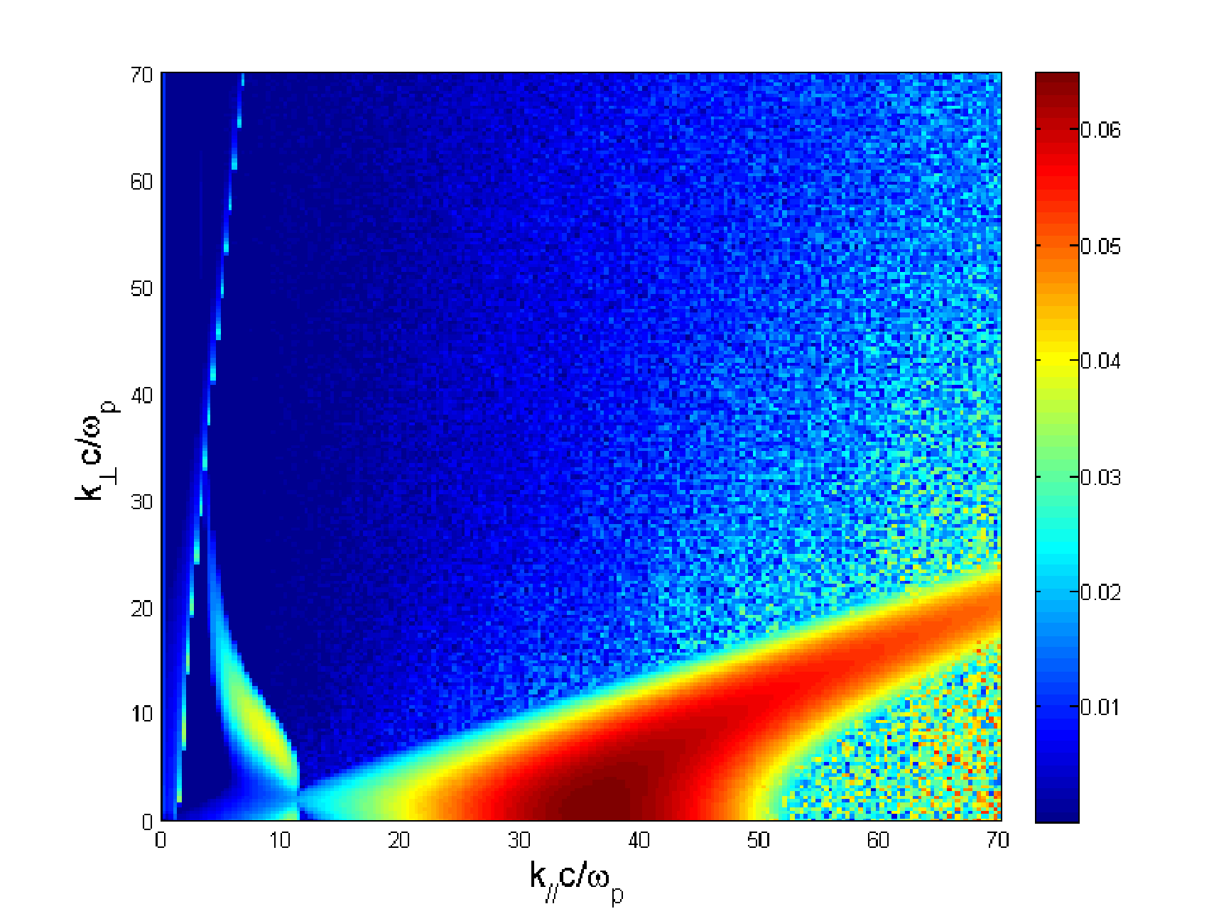
Figure 2: The exponential growth rate of the linear instability in units of $\omega_{p2}$ for the ion-to-electron mass ratio $R=250$ used in the simulation. The wavenumbers are normalized to the skin depth $\lambda_{2}$ of the dense ion species.

The exponential growth rates peak in the field-aligned direction, which is characterized by a wavenumber component along the beam velocity vector $k_{\parallel}\lambda_{2}\neq 0$ and a perpendicular component $k_{\perp}\lambda_{2}=0$. These modes could be observed in a 2D simulation of an oblique shock, which employed a lower collision speed (Dieckmann et al. 2010). However, the modes with $k_{\perp}\lambda_{2}\neq 0$ are not suppressed. Bands of unstable waves reach out to $k_{\perp}\lambda_{2}\gg 1$. The shock and its downstream region may thus not be planar. According to this solution of an idealized linear dispersion relation, the structuring of the shock along its boundary is captured well by a simulation box that spans a few ion skin depths into this direction and resolves the electron skin depth. Our simulation will represent the wavenumber band $1\sim k_{\perp}\lambda_{2}<134$. The growth rate map for the mass ratio $R$ is qualitatively similar to that obtained for the correct proton-to-electron mass ratio (not shown), which suggests that the spectrum of unstable waves in the PIC simulation will be realistic, at least during the initial time. This is not always the case for reduced mass ratios (Bret & Dieckmann 2010).

2.3 Numerical resolution and computational details

For the 2D simulation, the box measured in ion skin depths is of width $L_{x}=656\lambda_{2}$ and of height $L_{y}=6\lambda_{2}$ resolved in $2.8\times 10^{4}$ cells in the propagation direction and 256 cells in the perpendicular direction. The total plasma Debye length $L_{T}$, where $\frac{1}{L_{T}}^{2}=\frac{1}{L_{D,ion}^{2}}+\frac{1}{L_{D,electron}^{2}}$ is resolved in 1 cell in the simulation. The electron skin depth is resolved in 2.7 cells. We use 200 computational particles per cell (100 ions, 100 electrons) in the dense plasma and 100 particle per cell (50 ions, 50 electrons) in the tenuous plasma, which is possible by assigning different numerical weights to the CPs. No new particles are introduced at the periodic boundaries during the simulation. The two plasma clouds rapidly detach from the boundaries. The high thermal speed of the electrons implies, that they leave the plasma clouds at their rear ends to leave behind a positive net charge. This charge separation induces an electric field, which accelerates the ions. This process has been researched in the context of a plasma expansion into a vacuum (Mora & Grismayer 2009). While such an expansion clearly is an artifact of our initial conditions, it does not visibly influence the plasma dynamics at the collision boundary. This will be demonstrated below by the supplementary movies, which do not show waves or plasma structures that propagate from the simulation box boundaries to the cloud collision boundary in the center of the simulation box. The x-boundaries are intentionally placed sufficiently far from the shock forming region that no signal can reach the shock forming region traveling from the boundaries within the simulation time.

The number of processors used was 256 Intel Xeon E5462 2.8GHz on an ICHEC SGI ICE machine (Stokes). Total wall clock time was $156$ hours, giving a cumulative CPU time of $\sim 40,000$ hours for the 2D simulation.

3 The simulation results

In this section we elucidate the consequences of two plasma clouds colliding. Although the plasma dynamics in the cloud overlap layer is determined by both clouds simultaneously, we will analyse them separately. This is made possible by tagging the CPs initially belonging to the species under consideration. Henceforth we shall refer with dense ions/electrons to the corresponding species of the dense cloud that moves to the right, while the tenuous ions/electrons are those of the diluted plasma cloud that moves to the left. In order to gain insight into the growth of structures due to the interaction of the clouds, we present results of a numerical simulation at the early time of $T1=62$ and the later time of $T2=182$. The static images are supported by animated MPEGs available in the online edition, which show the time-evolution of the fields.

3.1 Early stage at time T1

At the time T1, the beams have counterstreamed for tens of ion skin depths. We look first at the electron phase space distribution integrated over $y$. The dynamics of the electron beams show that the electrons at position x=30 are already accelerated to $\Gamma=60$ from the initial $\Gamma\leq 8$ (Figure 3). The strongest electron acceleration occurs for $30<x<33$. The relativistic inertia of these electrons is already comparable to that of the ions and we expect a detectable reaction from them. From the ion phase space plot in Fig. 4, which is also integrated over $y$, it can be seen that little interaction has taken place in between the colliding clouds of ions over most of the displayed $x$-interval. However modulations of the specific x-momentum of both clouds are highly evident at $30<x<40$. All ions are decelerated at $30<x<33$ in the simulation frame, which provides a reservoir of energy for the acceleration of electrons and dense ions to $\Gamma v_{x}\approx 1.2$ at $x\approx 32$. The dense ions are decelerated also at $x>35$.

The large-scale distribution of the ion densities is shown in Fig. 5 for the tenuous ions and dense ions. The tenuous ions undergo a rapid filamentation, as they reach the cloud overlap layer at $x\approx 40$. The tenuous ions initially form filaments with a thickness of $\approx 0.1$ that are almost aligned with the flow velocity vector. Assuming the current channels are engendered by a filamentation instability between the ions of both clouds without electron involvement, one should see such structures also in the dense ions. This is because both clouds have approximately the same density and temperature for $30<x<40$ and both should thus behave similarly. Filamentary structures resembling those in the tenuous ions are, however, not visible in the dense ions on this scale. This filamentation instability must thus involve all plasma species. The electrons in this interval still carry a substantial directed flow energy, which can be released and further modify the instability. At this advanced simulation time, the linear dispersion relation discussed above would no longer be a good approximation. However, the key conclusion we draw from it, namely that the filamentation instability is not suppressed, is supported by the ion distribution.

The current channels in the tenuous ions are then rapidly deflected and thermalized, as they enter the interval $30<x<33$ in Fig. 5, where the electron acceleration and, thus, the electromagnetic fields are strongest. A structured and beamed distribution is present for $x<30$. The ions in these channels have not decreased significantly their $p_{x}$ momentum (Fig. 4). A two-dimensional density modulation is also visible in the dense ions for $-20<x<30$. Its density peaks at $x=30$, which is the interval where the dense ions are slowed down most in Fig. 4. The planar front of the dense cloud is surrounded by filamentary distributions, as it has also been observed for a reduced collision speed (Dieckmann et al. 2010).

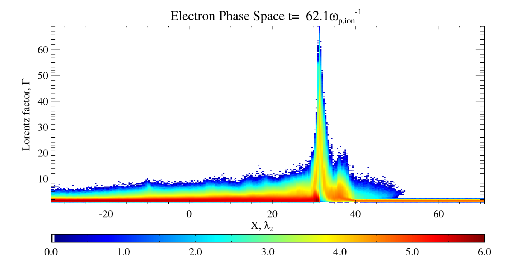
Figure 3: Electron phase space: Log of electron density as a function of Lorentz factor $\Gamma$ and x at time $t=T_{1}$.

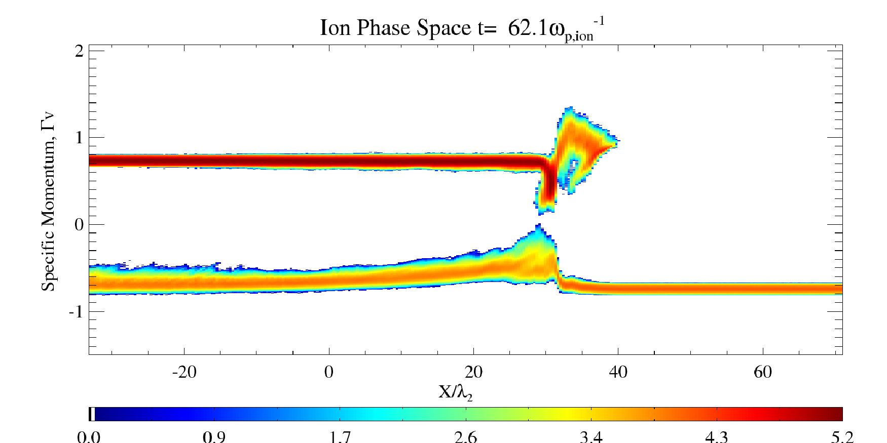
Figure 4: Ion phase space: Log of ion density as a function of specific x-momentum $\Gamma v_{x}$ and x at time $t=T_{1}$

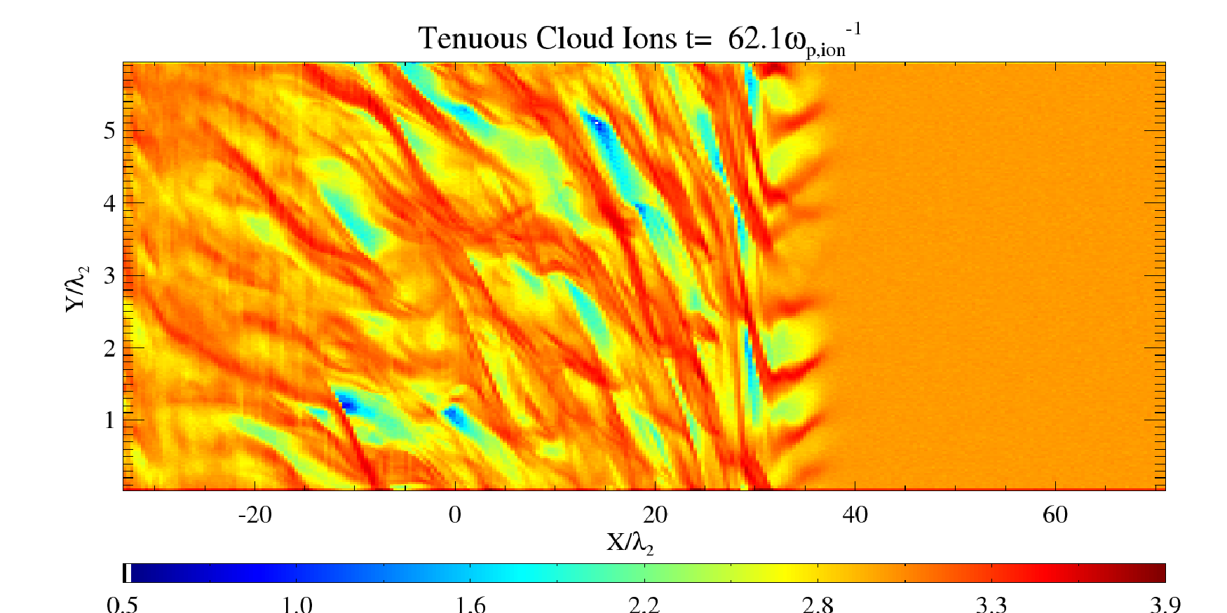
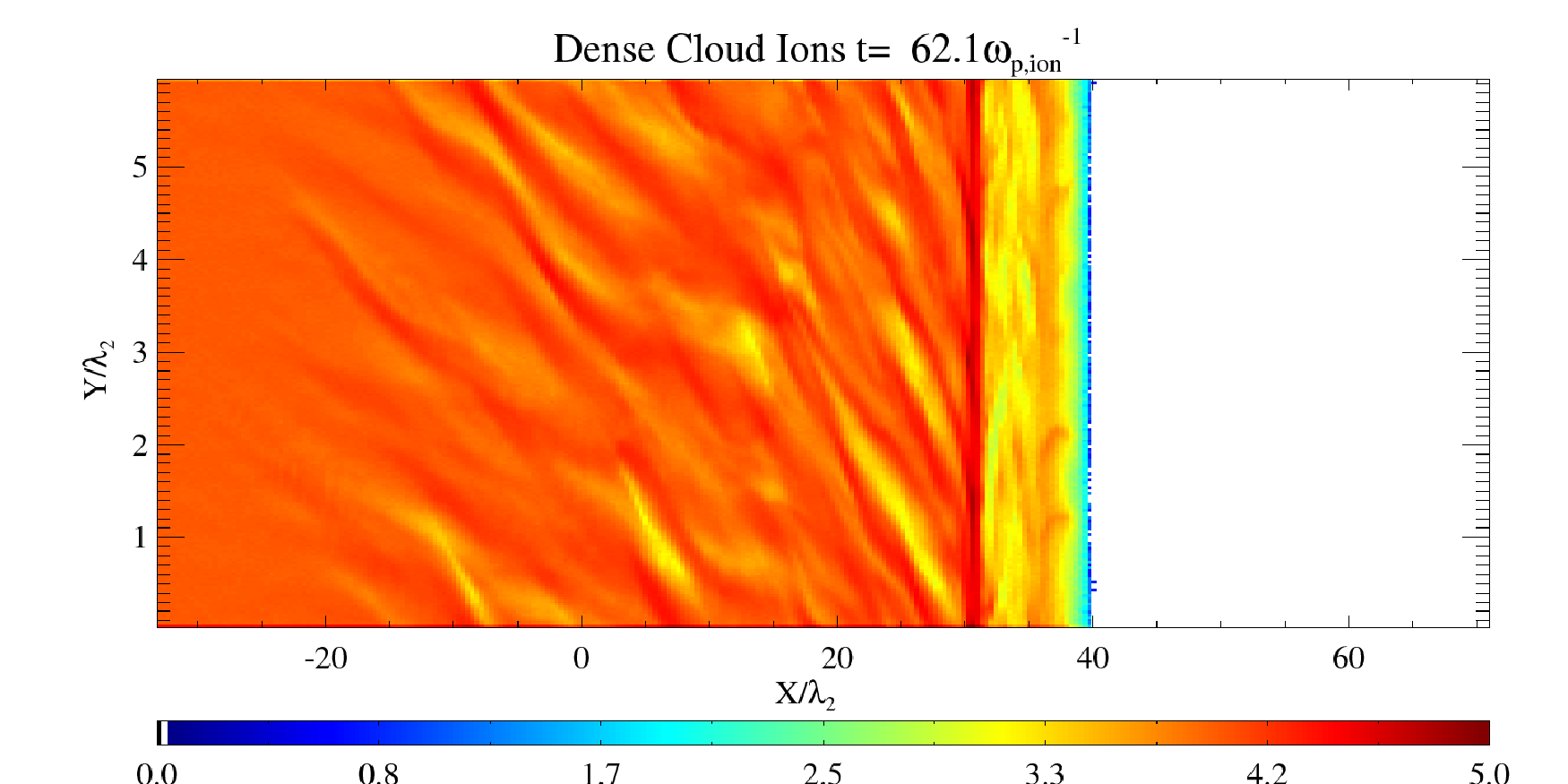
Figure 5: Two dimensional logarithm of the ion density as a function of X and Y at the time $t=T_{1}$. The upper panel shows the left moving tenuous ions and the lower one the right-moving dense ones.

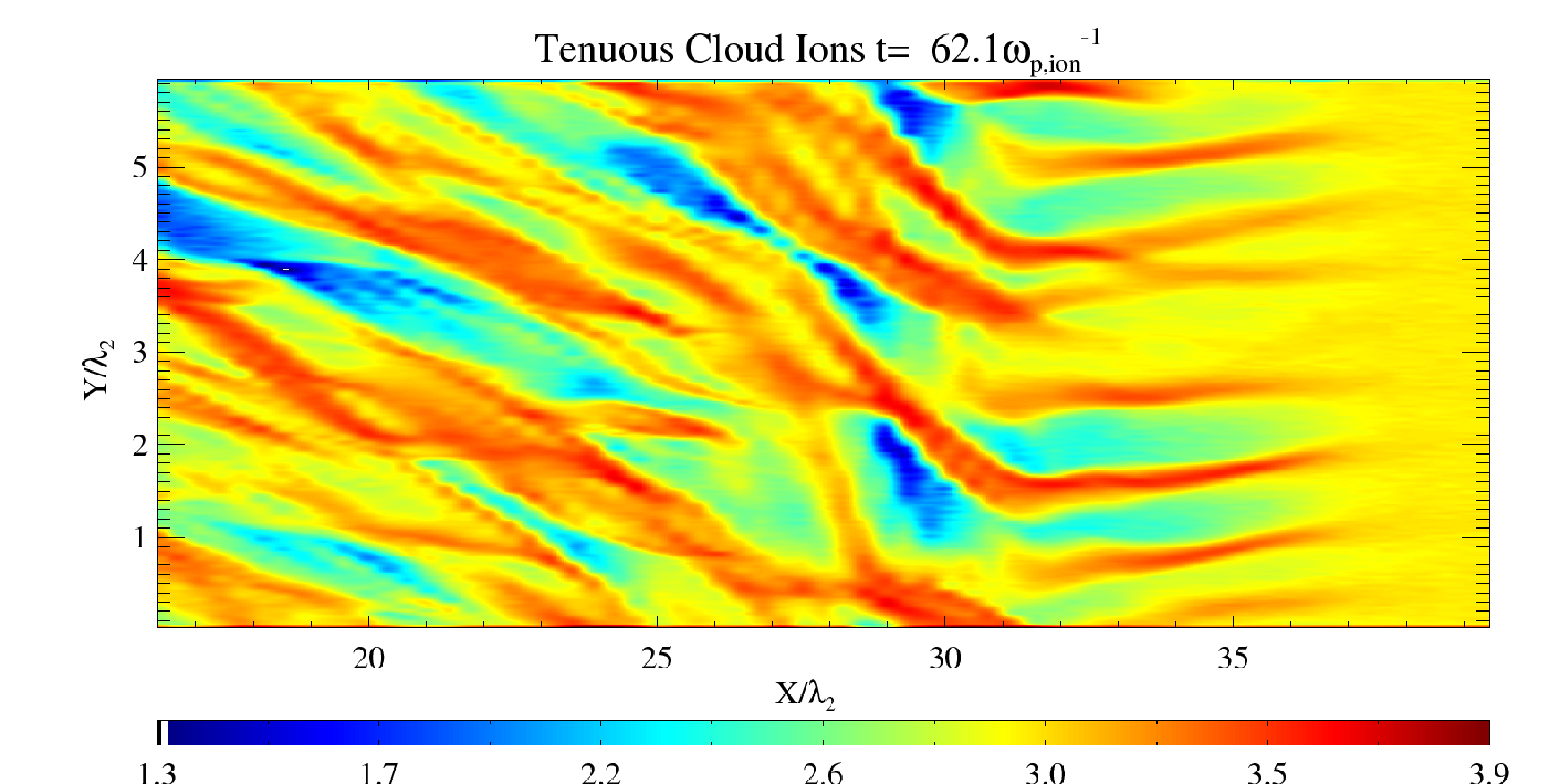
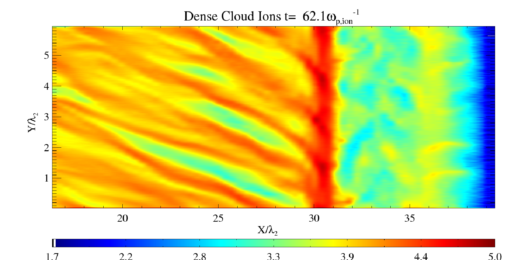
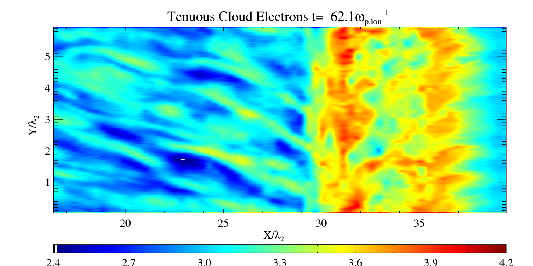
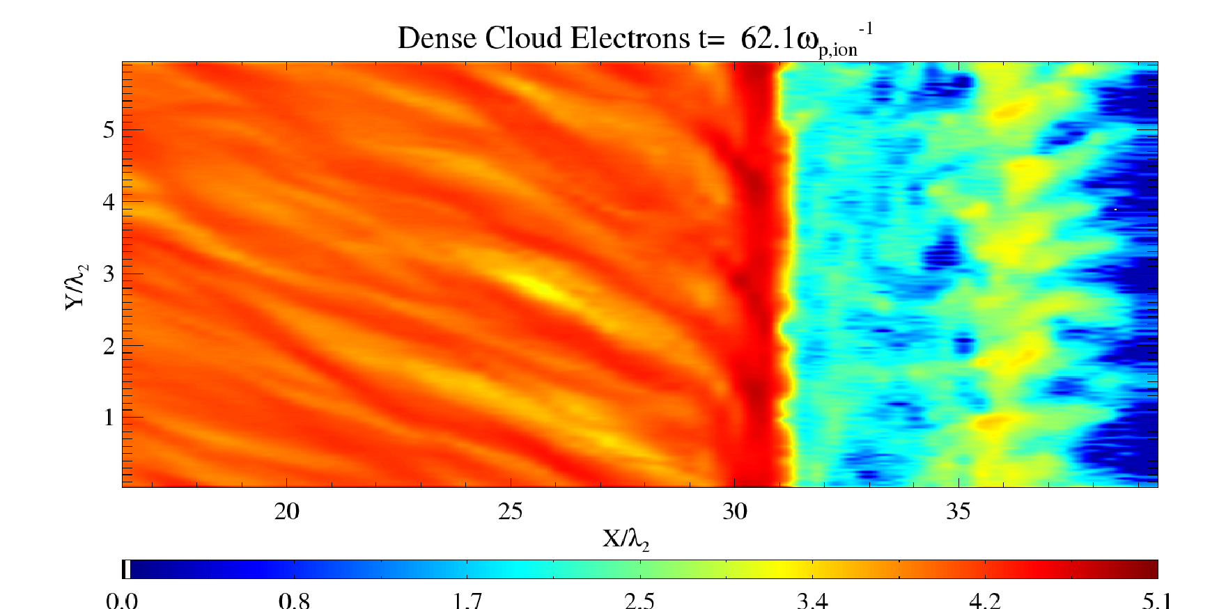
Figure 6: Two dimensional plots of logarithm of dense and tenuous ion and electron clouds at time T1, for the zone close to the collision boundary.

A zoom of the zone around the collision boundary (Figure 6) shows the spatial density distribution of each of the four species. The current channels in the tenuous ions start to form at $x\approx 38$. The current density increases as we go from this position to $x\approx 34$ and the space between the channels is progressively depleted of ions. The current channels merge, e.g. at $x\approx 33$ and $y\approx 4$. Only 4 major current channels eventually cross the electron acceleration region and reach $x\approx 30$, where they are deflected to increasing values of $y$ and scattered at $x\approx 27$. Remarkable density modulations of the tenuous ions are visible at $x\approx 30$, where we find a minimum density of $\exp{(1.3)}\approx 4$ at $y\approx 1.7$ and a maximum density of $\exp{(3.9)}\approx 50$ at $y\approx 2.5$. Their density minima at $(x,y)=(29.5,1.7)$, $(30,3)$ and $(30,5.5)$ are correlated with local maxima of the density of the dense ions. Some correlations between the filaments of the tenuous and the dense ions are visible, e.g. at $x\approx 37$ and $y\approx 1$ and $y\approx 2$, where the current channels both have a density of $\approx\exp{(3.5)}$.

The dense ions show a quasi-planar front at $30<x<31$ with an enhanced density as well as a less pronounced second front at $x\approx 36$. In particular the front at $x\approx 31$ is sharp and the densities of the dense ions and electrons decrease by a factor $\approx 5$ and $\approx 20$, respectively, as we cross its boundary to the upstream (larger $x$). The lower density of the dense electrons ahead of the front is probably caused by their rapid expansion upstream. Figure 3 reveals that hot electrons leak out of the acceleration region and reach a $x\approx 50$. Their current induces a return current in the tenuous electrons, which accelerates the latter towards the density peak at $x=31$ and results in their accumulation at $30<x<33$ and at $35<x<38$. The dense electrons also accumulate in $35<x<38$. The density maxima of the tenuous electrons correlate well with the locations, where the electron acceleration in Fig. 3 and the ion deceleration in Fig. 4 is strongest. The ion deceleration in the interval $35<x<38$ causes their accumulation and also that of the electrons, which must cancel the ion charge. Furthermore, a strong filamentation along $y$ is visible for $20<x<30$ for all four species in Fig. 6.

The mechanisms that accelerate the electrons at the expense of the ion energy can be identified with the help of the electromagnetic fields. The magnetic and electric components in the location of the collision boundary (Figures. 7 and 8) reveal a large electromagnetic pulse in the interval $30<x<33$, which is the interval with the strongest electron acceleration and ion deceleration in Figs. 3 and 4. The electromagnetic fields orthogonal to the collision (x) direction reveal bipolar pulses, which are shifted in space. This is most evident for $B_{y}$, where the negative and positive magnetic field is separated at $x\approx 31.5$. This zero crossing of $B_{y}$ is approximately where $B_{z}$ reaches its maximum positive value, evidencing a phase shift of $90^{\circ}$ along $x$ between $B_{y}$ and $B_{z}$. A negative $B_{z}$ is then visible at $x\approx 33$, just ahead of the positive interval of $B_{y}$. The $B_{y}$ and $B_{z}$ reach moduli $\approx 100$ each, which is about 6 times larger than $|\mathbf{B}_{0}|=250^{1/2}$.

The bipolar pulse of $E_{y}$ is in phase with that of $B_{z}$, while the pulse in $E_{z}$ is in antiphase with that in $B_{y}$. The electric field pulse is to some degree the consequence of the rapidly moving magnetic field pulse (convection electric field) and this contribution would vanish in the rest frame of the magnetic field structure moving with the speed $\approx v_{b}$. The $B_{y}$ and $E_{z}$ show a further oscillation at $x\approx 35$, suggesting that it is the same circularly polarized energetic electromagnetic structure that was observed previously by Dieckmann et al. (2008, 2010), although here its coherency along $y$ is low and it does not extend far upstream. The low coherency can at least in parts be attributed to the strong spatially varying $B_{x}$. The presence of a strong nonplanar $B_{x}$ implies spatially varying strong currents in the z-direction.

A single circularly polarized purely electromagnetic wave cannot by itself accelerate electrons to ultrarelativistic speeds. Its combination with the electric $E_{x}\gg 0$ in Fig. 8 is necessary for this purpose. In our normalization the ratio of the values for $\mathbf{E}$ and $\mathbf{B}$ is almost equal to the force ratio for a particle, which moves with $v\approx c$. The electric and magnetic forces on relativistic particles are thus comparable. The $E_{x}>0$ can be explained as follows. As the upstream plasma impacts on the strong magnetic field at $x\approx 33$, the electrons are deflected away from their original flow direction, while the ion reaction is much weaker. A current develops in the y-z plane, which amplifies locally the magnetic field. The electrons fall behind the ions, because their velocity along $x$ is reduced. An $E_{x}>0$ builds up, which tries to restore the quasi-neutrality. The tenuous electrons are dragged by it across the magnetic field. This cross-field transport accelerates the electrons to relativistic speeds, as it is confirmed in Fig. 3. This acceleration acts in the y-z plane, which partially explains the spatial confinement along $x$ of the accelerated electrons. This spatial confinement of the strong electromagnetic fields and of the electron acceleration also implies a localized fast decrease of the ion flow speed, explaining the ion reaction within $31<x<35$ in Fig. 4. The electric field, which drags the electrons to the left in this interval, causes the slowdown of the tenuous ions as they move to the left and the speedup of the dense ions, which move to the right. The consequent ion accumulation further confines with its massive positive charge the electrons. This electron acceleration mechanism ceases to work, when the $E_{x}$ is strong enough to stop the ions.

We can also observe filaments in particular in $B_{z}$ for $x<30$, which results out of the filamentary strucures observed in all plasma species in this interval. We expect this magnetic component to show the strongest modulation if the currents are approximately aligned with the $x$-direction and are modulated along $y$. Magnetic field stripes aligned with $x$ are also observed for $x>35$. These filaments are driven by the upstream electrons and the electrons that leak to higher $x$, reaching $x\approx 50$ in Fig. 3. This upstream filamentation has also been observed at the faster shock modelled by Martins et al. (2009).

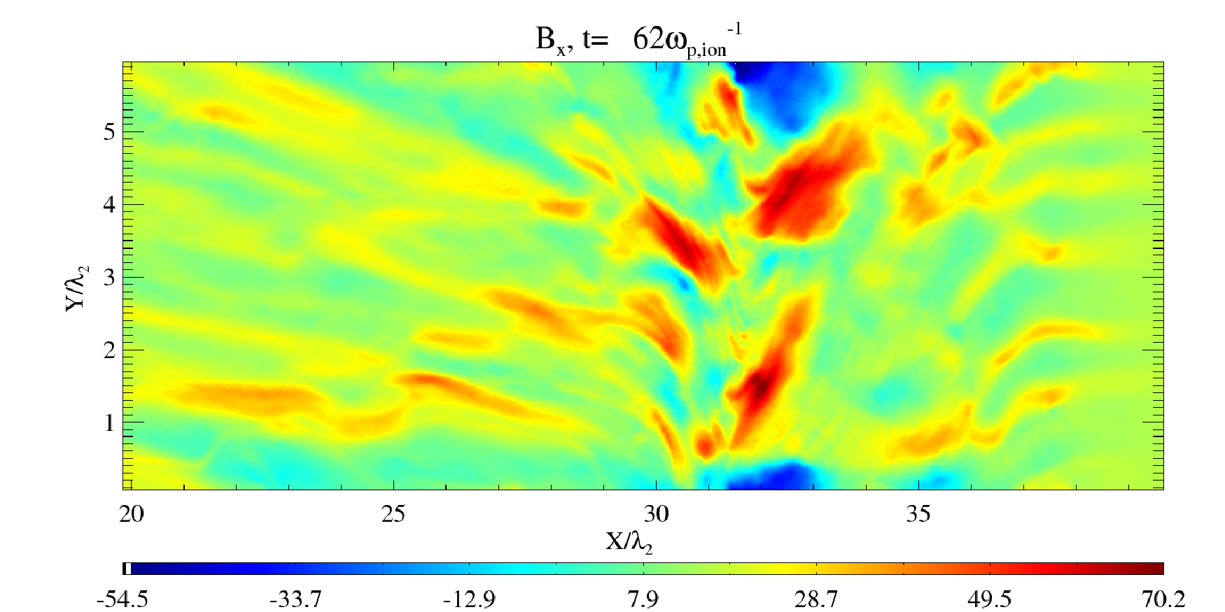
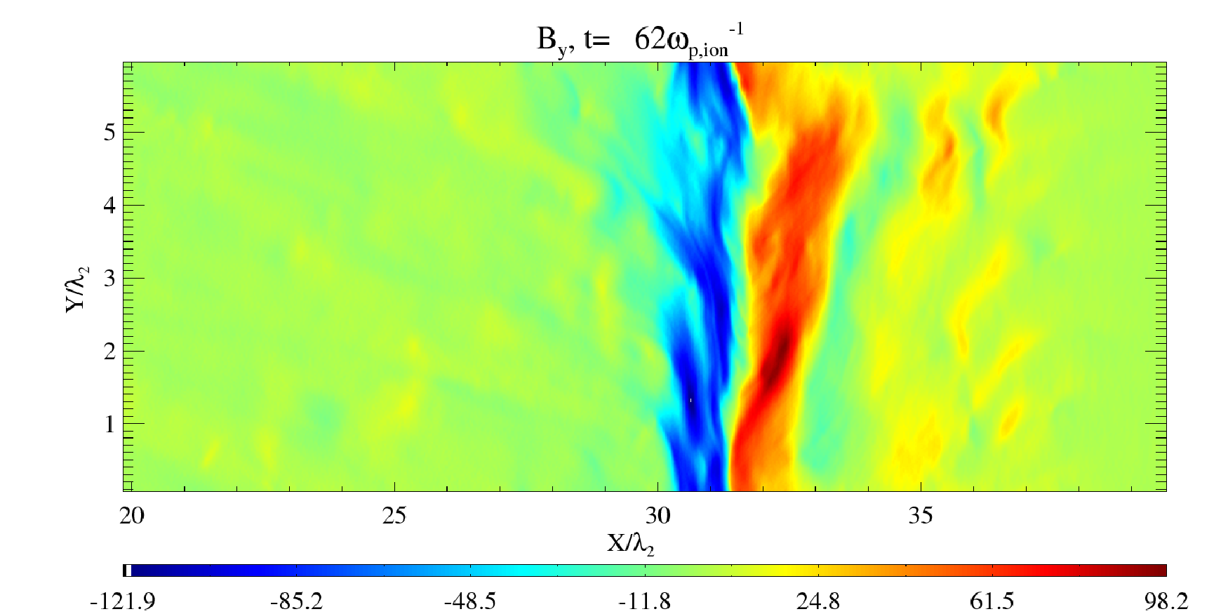
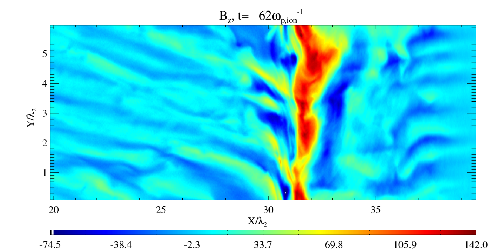
Figure 7: Magnetic field components: Zoom of 2D linear colourscale plot of spatial distribution of $B_{x}$ (upper plot), $B_{y}$ (middle plot) and $B_{z}$ (lower plot) at $t=T_{1}$.

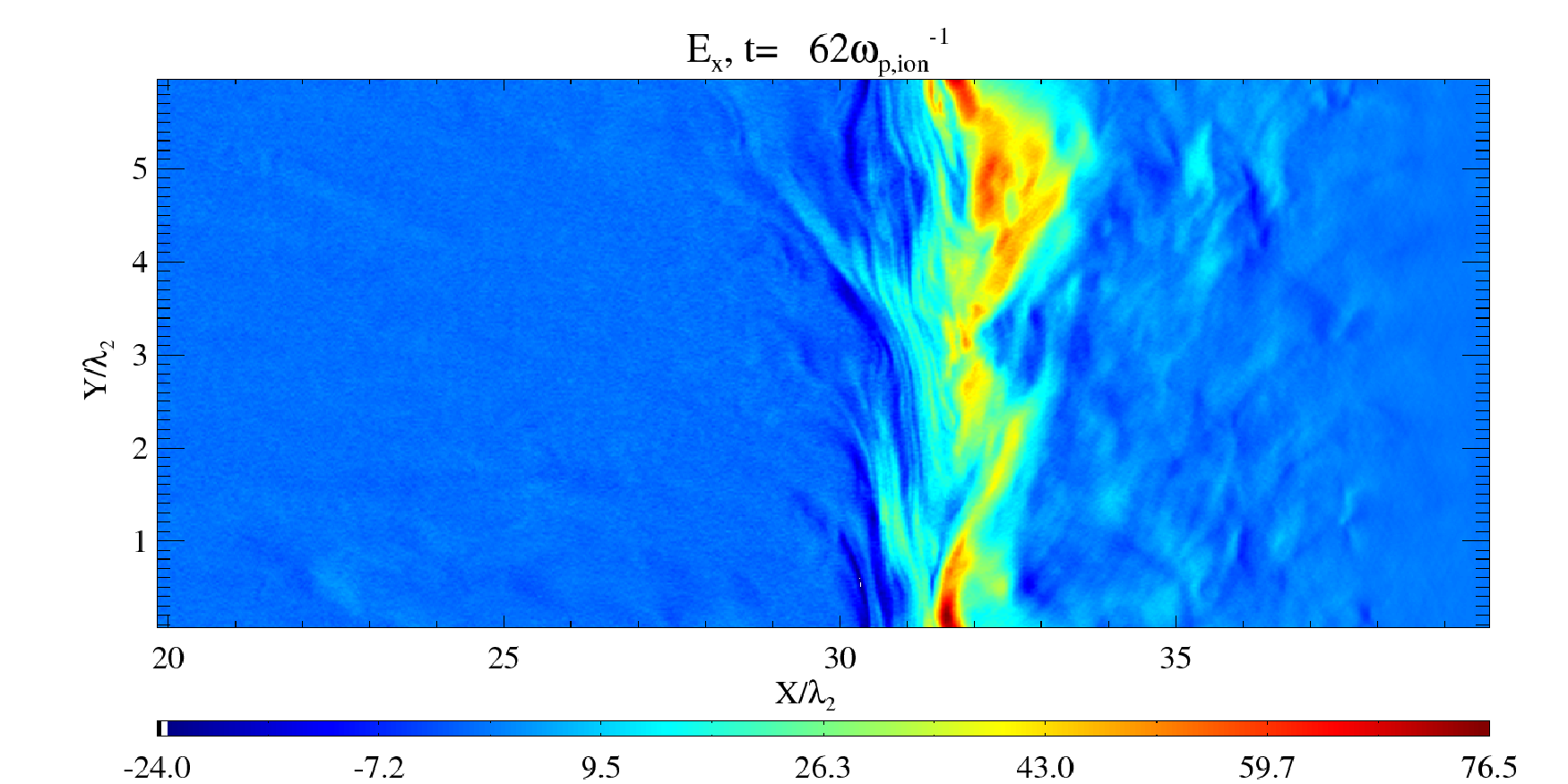
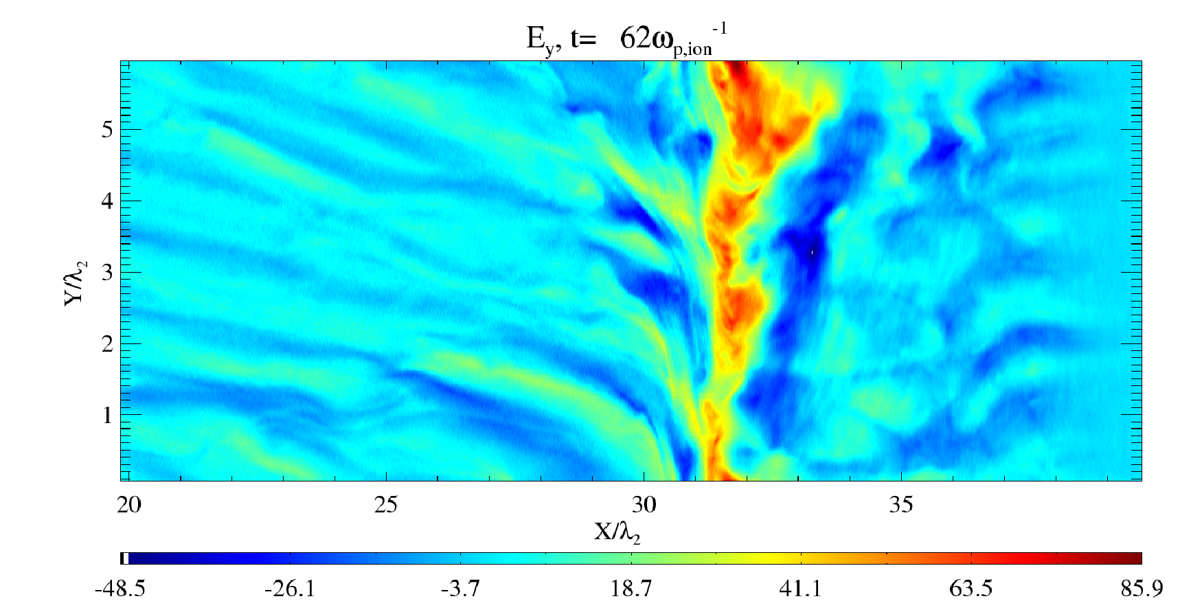
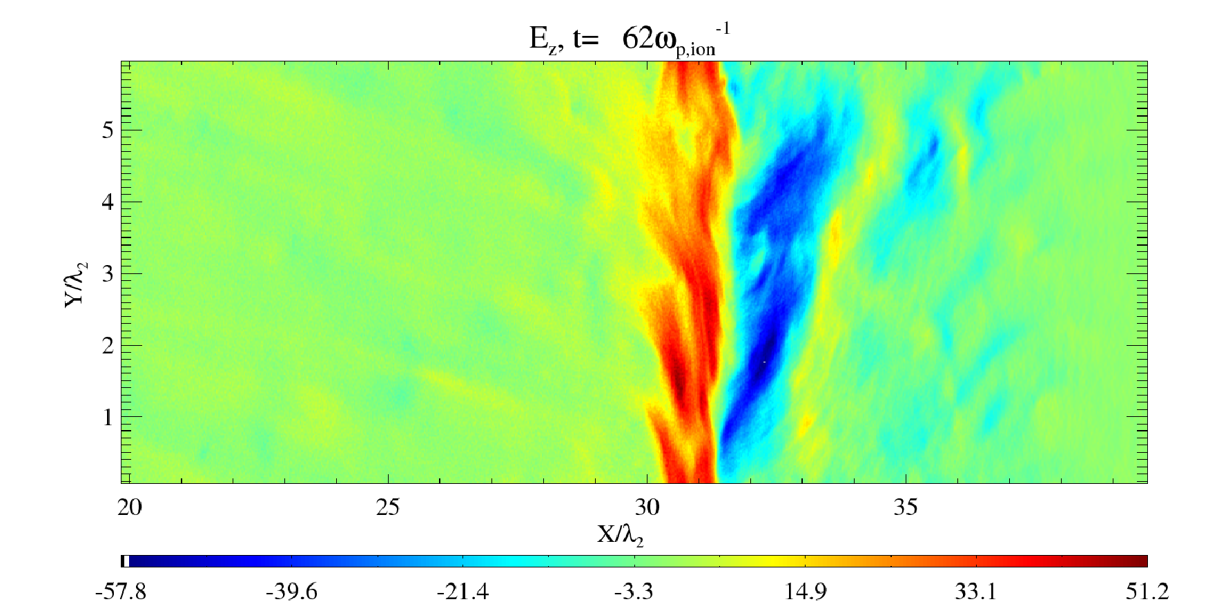
Figure 8: Electric field components: Zoom of 2D linear colourscale plot of spatial distribution of $E_{x}$ (upper plot), $E_{y}$ (middle plot) and $E_{z}$ (lower plot) at $t=T_{1}$.

3.2 Late stage

The physics at time T1 has given us insight into the plasma processes that take place initially and precondition the plasma such that the vortex forms, which is discussed in detail in MDD. We now consider the simulation time T2, which is approximately that investigated in MDD. Here we discuss in more detail the electromagnetic fields at the shock front, which have not been shown in MDD. The fields may not provide more information related to the vortex than the current, but they are essential to understand the particle acceleration, which is the focus of this paper.

To aid the analysis, in the simulation three distinct zones are identifiable at T2. These zones are most easily distinguished in Fig. 9, which displays (as in Fig. 4) the ion phase space density integrated over $y$ as a function of $x$ and $p_{x}$, but now at the time $T_{2}$. The displayed x-interval can be subdivided into the interpenetrating ion beam zone (IIBZ) with $-35<x<60$, the downstream region with $60<x<80$ and the foreshock region of the strong forward shock with $80<x<130$. Fig. 4 and Fig. 11 are show a similar time slice to Fig. 2 in MDD.

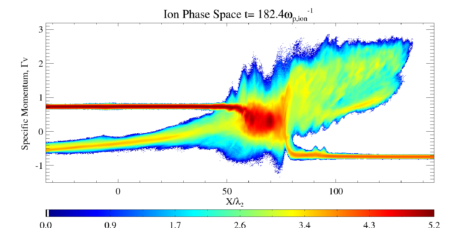
Figure 9: Ion phase space: Logarithm of electron density as a function of specific x-momentum $\Gamma v_{x}$ and x at $t=T_{2}$.

First we note that the strongest interaction takes place at $x\gg 0$ and that it is tied to the front end of the dense cloud. No energetic structure is visible at the front end of the tenuous cloud (not shown). The incoming plasma from the upstream, here the tenuous cloud, is reflected at $x\approx 80$, forming a shock-reflected ion beam. This shock reflected ion beam is hot and the reflection is not specular. A bunch of ions with values of $p_{x}$, which are comparable to the initial ones of the dense ions, is visible in the interval $100<x<120$. These are the dense ions, which were located ahead of the strong interaction region found at $x\approx 33$ in Fig. 4, and they have not been accelerated by it. The downstream region is characterized by a single, almost spatially uniform and hot ion population. The kinetic energy stored in the relative speed between the upstream and the downstream plasma has been converted into heat. The momentum conservation, together with the asymmetric cloud densities, implies that the downstream region cannot be stationary in the box frame. Indeed, the normalized mean speed along $x$ of the downstream ions is $\approx 0.33$ according to Fig. 10, while the speed modulus of both incoming clouds is the same in the simulation frame of reference. The speeds of the observed forward shock that is moving to the right and the reverse shock that is still developing, which are given by the relative speed between the downstream plasma and the respective upstream plasma, must differ.

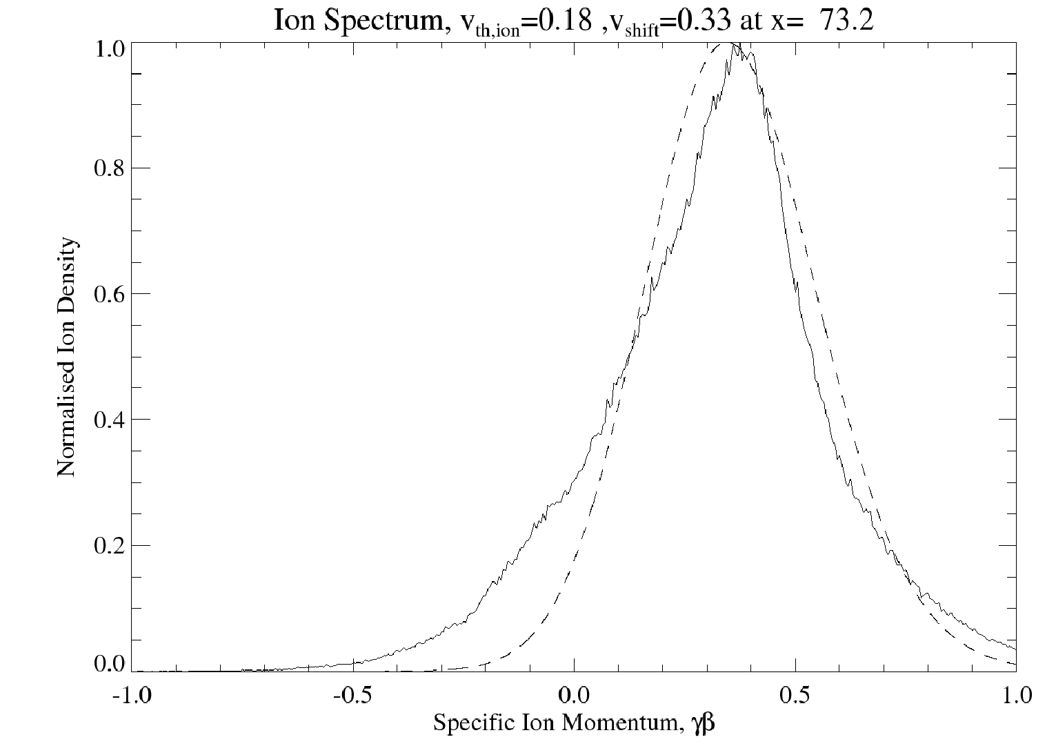
Figure 10: Ion momentum distribution at $x=73.2$, normalized to its peak value, at $t=T_{2}$. A fit to a Maxwell-Jüttner distribution with the thermal speed 0.18c and the mean speed 0.33c is overplotted.

The IIBZ to the left is characterized by the co-existence of the dense ions and the tenuous ions, which have crossed the front of the dense cloud prior to the formation of the shock. The mean speed modulus of the tenuous ions increases as we go to lower $x$ and it is close to the initial one at $x\approx-35$. This spatially varying mean momentum is a consequence of the shock formation. The mean speed modulus of the tenuous ions in the strong interaction region decreased steadily in time, as the electron acceleration became more efficient. The later in time the tenuous ions traversed this strong interaction region, the more energy they lost to the electrons. Once the downstream region has been formed, the tenuous ions can no longer cross this obstacle. The tenuous ion beam in the IIBZ is thus a transient effect. Eventually, a reverse shock will form between the IIBZ and the downstream, giving rise to a shock-reflected ion beam.

Movie 1 shows a zoom of the time evolution of the ion distribution in $(p_{x},x)$ space. We note that no signal, either wave or plasma structure is detected propagating into the box either from left or right boundaries. The early stage shows two beams colliding. The beams interpenetrate and then decelerate and a forward shock begins to form. The tenuous beam is partially reflected to high velocities by the dense beam. Left of the collision boundary, the structure is clearly heated and takes on a thermal distribution (fitted to a Maxwellian in Fig. 10). The lower panel shows the left moving cloud ion distribution in $(x,y)$ space. The most significant structures at early times are the distinctive filaments, which dominate both the foreshock and the downstream region. The filaments are sheared in the negative y direction and circular structures are seen to form which increase in size at the later stage of the simulation, to eventually fill the simulation box, at which point we stop the simulation.

Figure 11 displays the electron phase space density distribution as a function of $x$ and $\Gamma$ at $T2$.

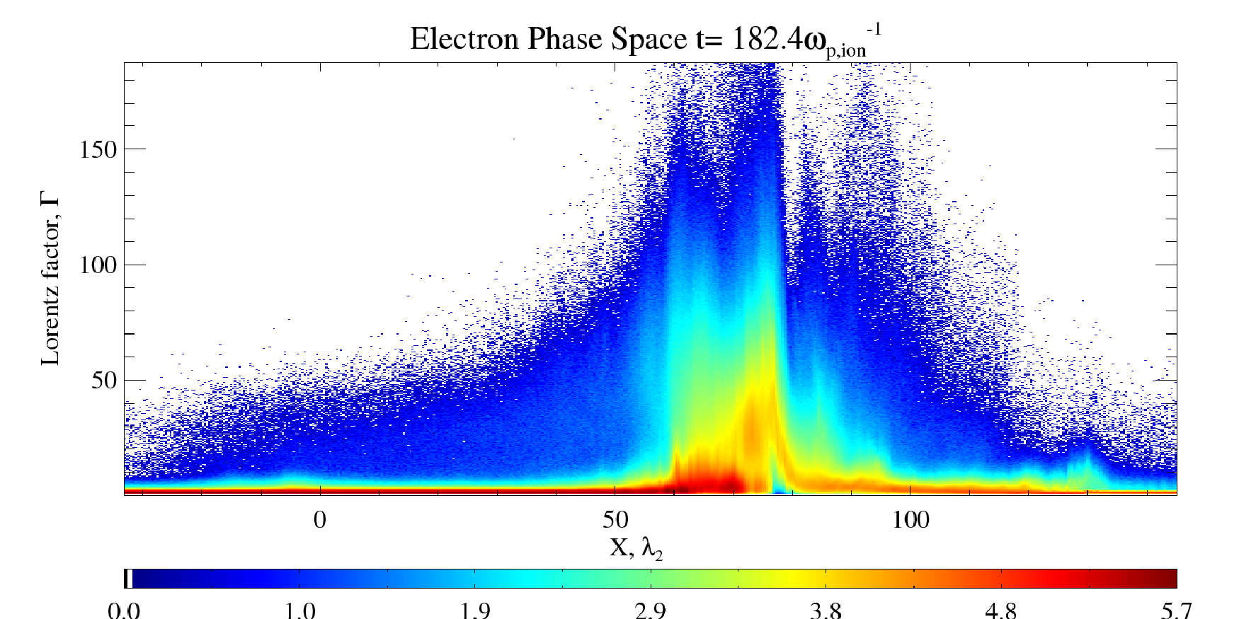
Figure 11: Electron phase space distribution at $t=T_{2}$: Logarithm of electron density as a function of the Lorentz factor $\Gamma$ and x.

The downstream region hosts a hot and dense electron population. The strongest electron acceleration takes place at the boundary between the downstream region and the foreshock at $x\approx 80$. The most energetic electrons reach $\Gamma>180$. Their relativistic energies are well above that of an ion with 250 electron masses and the speed $v_{b}$. The latter would have a kinetic energy, which would equal that of an electron with $\Gamma\approx 70$. A dilute cloud of ultrarelativistic electrons is leaking out from the downstream region into the foreshock region and into the IIBZ region. The distribution of the dense electrons in the IIBZ is practically unchanged and clearly separated from the hot population, indicating that they are not interacting strongly through beam instabilities. The turbulent tenuous electrons in the foreshock with $x>80$ have probably been heated by the shock-reflected ions, since they are perturbed in the spatial interval up to $x\approx 130$, which coincides with the cut-off of the ion beam. Some interaction may have taken place in form of a filamentation instability between the leaking hot electrons and the incoming tenuous electrons, as it was observed at the time T1.

Movie 2 shows a zoom of the time evolution of the electron $(\Gamma,x)$ phase space in the upper panel, and the distribution of the left moving cloud in the lower panel. We note that no plasma structure enters the box from the left or right x- boundaries. The acceleration to ultrarelativistic Lorentz factors occurs in a confined region close to the collision boundary. Filamentation dominates but to a lesser extent than found in the ion clouds, due to the higher thermal velocities of the electrons in the foreshock. At later times, the same circular structure is seen as in the ion clouds.

The magnetic energy density at the time T2 is displayed in Fig. 12.

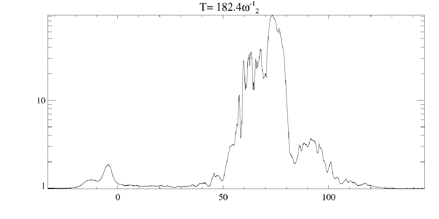
Figure 12: The total magnetic energy density B² at time T2 averaged over $y$ and normalised with respect to $|{\mathbf{B}_{0}}|^{2}$ plotted against x. The field is amplified to above 50 times its initial value in a thin layer, far above the value expected from a shock compression.

Elevated magnetic energy densities are observed in the IIBZ up to $x\approx 50$. Then the magnetic fields strengthen and reach a magnetic energy density plateau with $20{|\mathbf{B}_{0}|}^{2}$ at $x\approx 60$, which spans the downstream region up to $x\approx 70$. Then a massive peak is observed, reaching a peak value of $10^{2}{|\mathbf{B}_{0}|}^{2}$ at $x\approx 73$. The magnetic energy density decreases rapidly as we go from this position to increasing $x$ and it reaches a local minimum at $x\approx 85$ with the value $\approx 2{|\mathbf{B}_{0}|}^{2}$. The second weak maximum at $x\approx 90$ is followed by an apparently exponentially decreasing magnetic energy density that cannot be distinguished from ${|\mathbf{B}_{0}|}^{2}$ at $x\approx 125$. The absolute maximum of the magnetic energy density is found a few ion skin depths to the left of the $x\approx 77$, in which the upstream ions are reflected in Fig. 9 and where the electrons experience their strongest acceleration in Fig. 11. It is thus the magnetic ramp in Fig. 12 that is responsible for the particle acceleration, but the plasma structure responsible for the extreme magnetic energy density is located behind it. The position $x\approx 125$, beyond which the magnetic field is not visibly amplified, is approximately colocated with the front of the shock-reflected ion beam in Fig. 9.

The large magnetic energy density observed in Fig. 12 suggests, that the underlying currents must be due to the ions and we analyse their density distribution in Fig. 13.

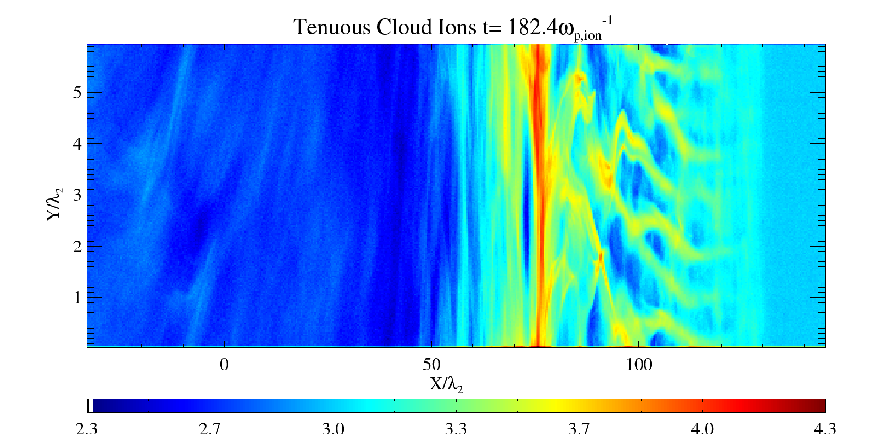
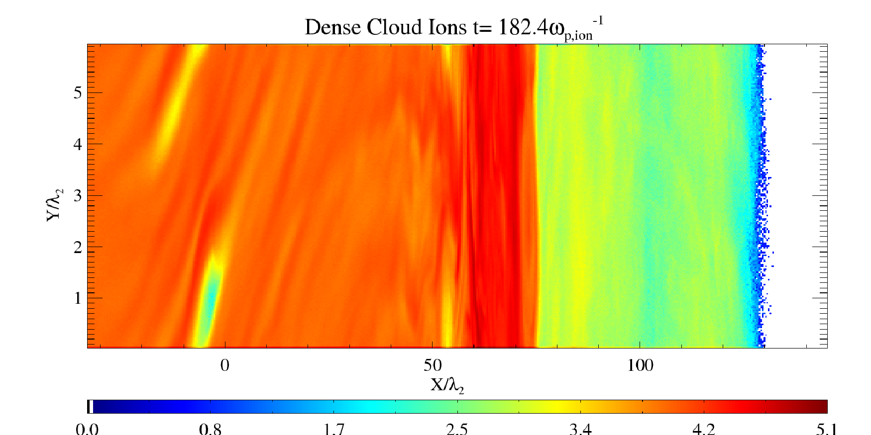
Figure 13: Two dimensional logarithm of the ion densities. The upper panel shows the left-moving tenuous ions and the lower panel the right-moving dense ions at $t=T_{2}$.

A structure is observed at $-10<x<0$ and $y<2$, which is periodically wrapped around at the boundary $y=0$. At the same position, we find a weak magnetic energy density peak in Fig. 12. A strong density depletion is only seen in the dense ions. The movie shows that this structure can be interpreted as the two-dimensional equivalent of a magnetic bubble. The interplay of the current filaments results in the accumulation of magnetic energy in a localized pocket, which is convected with the dense ions. The pressure gradient force of this magnetic bubble expels the dense ions. The tenuous ions move with a relativistic speed in the rest frame of this bubble and they and their density distribution are practically unaffected by the magnetic pressure gradient force.

The interval $50<x<73$ with the extreme magnetic energy is characterized by the increased ion density, which we expect to find in the downstream region of shocks. Note that the shock compression is not unusually high. The ratio between the downstream ion density $\approx\exp{(5)}$ and the upstream ion density $\approx\exp{(4)}$ (summed over both ion species) at the forming reverse shock at $x\approx 40$ is 3 in Fig. 13. The ratio between the downstream density and the upstream ion density at the forward shock at $x\approx 75$ is about 4. No current filaments are observed in this interval and it is unclear from this plot what is behind this immense magnetic energy density.

The tenuous ions show filamentary structures in the interval $80<x<130$, in which we find the weaker peak in the magnetic energy density in Fig. 12. This peak is thus due to the ion beam filamentation instability. The narrow well-separated filaments, which are stretched out over tens of ion skin depths, can be explained with a quasi-equilibrium similar to that derived for relativistic electron beams by Hammer & Rostocker (1970). No filaments can be found in the dense ions in this interval. The dense ions contribute to the fast beam, which outruns the forward shock, and this beam is too hot to react to the magnetic fields. The seemingly exponential growth in space of the magnetic energy density in Fig. 12 as we go from $x\approx 130$ to $x\approx 95$ may result from the combination of the exponential growth in time of the ion current in response of the filamentation instability with the convection to the left of the tenuous cloud.

Now we turn to a more thorough examination of the structure, which is responsible for the extremely strong magnetic field. It has previously been identified in MDD as a flux tube. Figure 14 displays the three magnetic field components at the time T2.

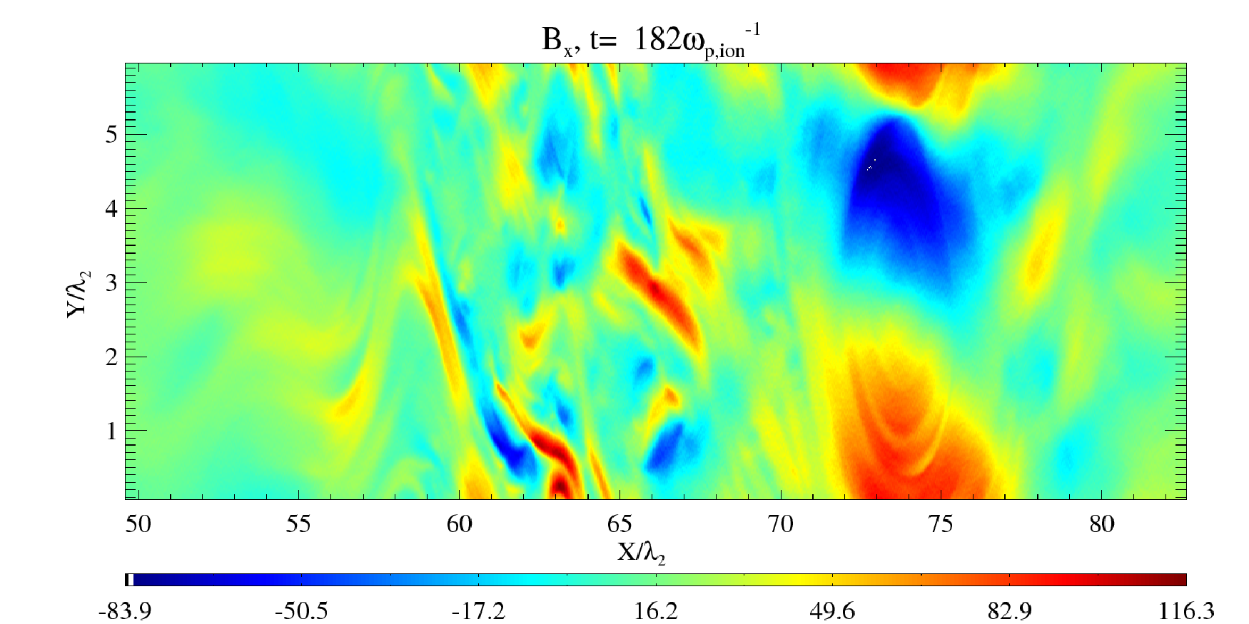
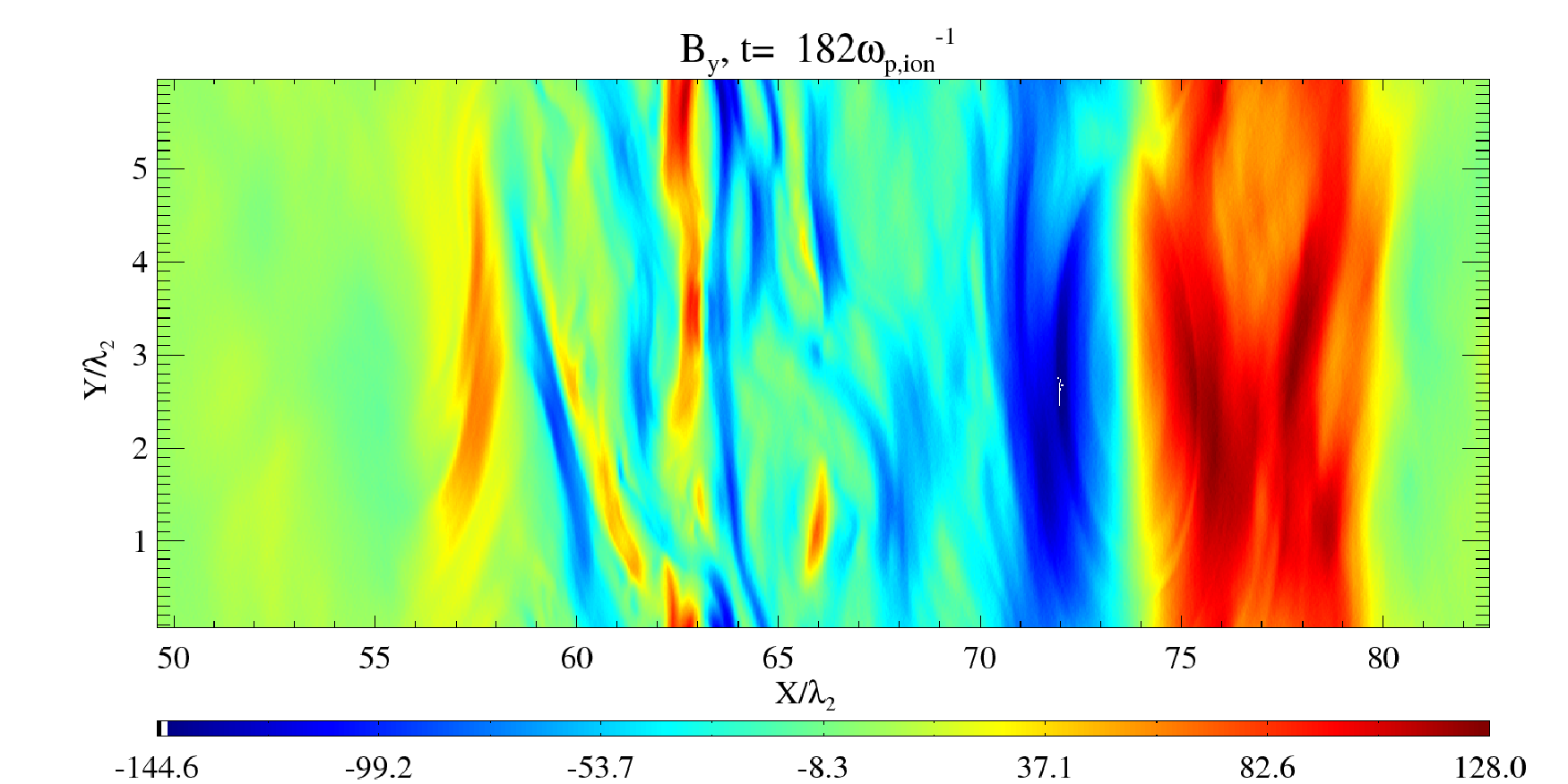
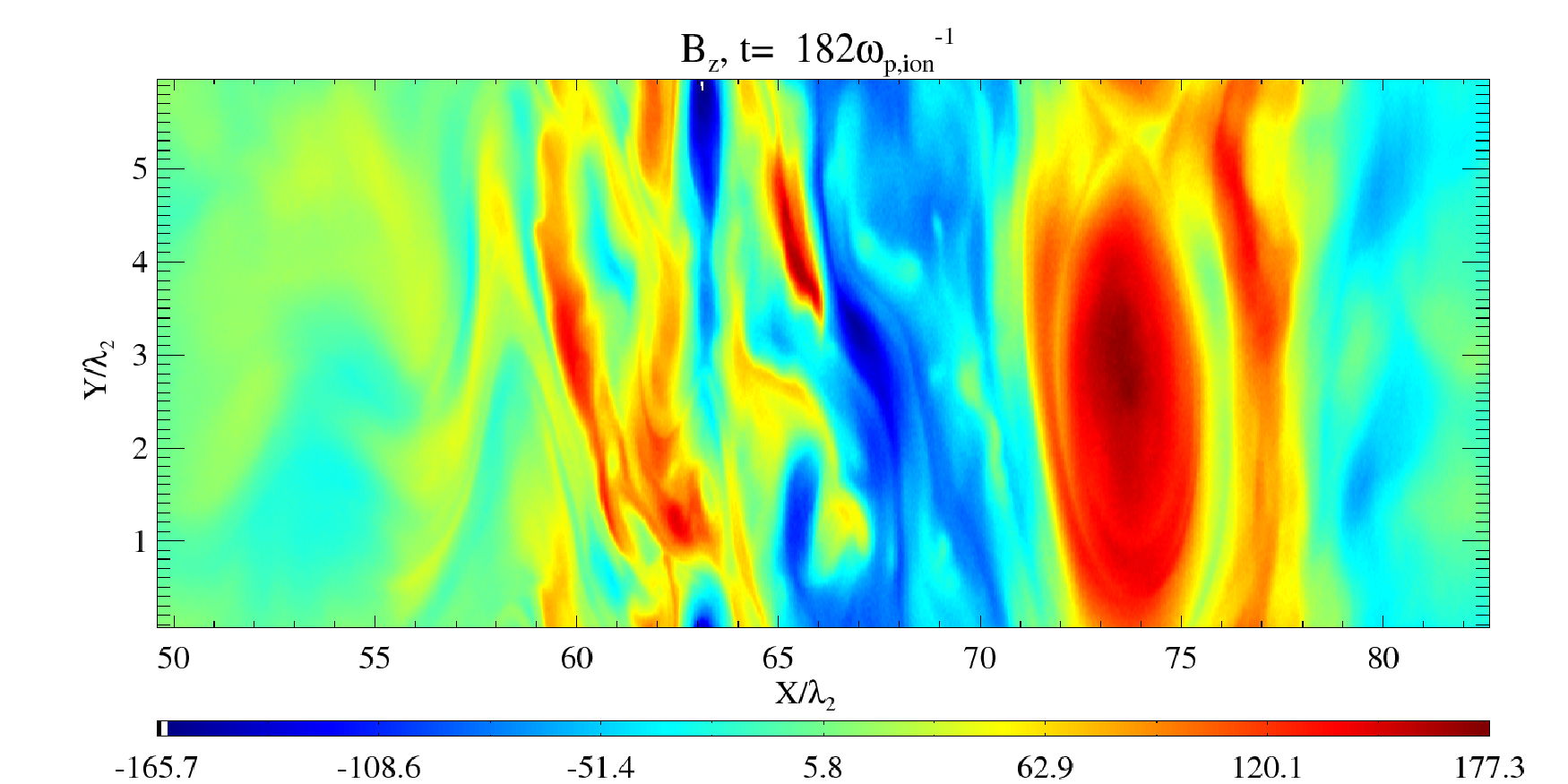
Figure 14: Magnetic field components at the time T2: Zoom of a 2D linear colorscale plot of the spatial distribution of $B_{x}$ (upper panel), $B_{y}$ (middle panel) and $B_{z}$ (lower panel).

The $B_{x}$ and the $B_{y}$ magnetic fields form a magnetic loop in the x-y plane for $70<x<77$, while the $B_{z}$ component reveals an elliptical structure within $71<x<76$. The simulation geometry implies that we can understand this magnetic field geometry as the combination of the axial magnetic field of a coil with an infinite extent along z and a magnetic ring that is surrounding it. Such flux tube distributions can be force-free, as they fullfill $\nabla\times\mathbf{B}=\alpha\mathbf{B}$ with a constant $\alpha$. If such a structure were to form in an astrophysical jet far from any magnetic source object, like what remains from the progenitor star, the magnetic field lines in the z-direction would have to be closed. A simple geometry that fullfills this necessary closure is a spheromak that resembles a smoke ring.

Apart from the dominant flux tube distribution, the magnetic field shows further elongated structures in the interval $55<x<70$. The geometry of these structures is reminiscent of the end product of the filamentation instability, which is apparently thermalizing the downstream distribution while maintaining the strong magnetic fields in this domain in Fig. 12. However, once the plasma has thermalized, these magnetic fields can no longer be upheld by plasma currents (Waxman 2006).

The strongest electron acceleration and the ion reflection by the forward shock takes place at $x\approx 77$, where we find magnetic stripes in the $B_{y}$ and $B_{z}$ components. These structures are not closed and resemble the bipolar pulse we have observed at the earlier time T1. If this bipolar pulse is responsible for the particle acceleration also at this late time, we expect to find a strong positive electric $E_{x}$ component at $x\approx 77$. Figure 15 confirms this. While the bipolar pulse is responsible for the electron acceleration and for the current sheet, out of which the flux tube has grown, the flux tube itself scatters through its magnetic field the electrons, as we can see from Fig. 11.

The separation of the flux tube from the current sheet driving it may have an important consequence. Figure 14 demonstrates that the periodic boundary conditions limit the growth of the flux tube. Selecting a simulation box that is much larger in the $y$-direction may result in a larger flux tube, but only if the further growth is not limited by the thickness of the current sheet along $x$. We would expect such a size limitation, if the flux tube could only exist in the current sheet. The current sheet would, of course, widen, if the simulation would model protons rather than the lighter ions. The thickness of the current sheet would, however, still be limited by the distance, over which the ion energy is depleted by the accelerating electrons. Here the simulation suggests that a current sheet ahead of the flux tube suffices to drive it. The flux tube can thus grow to a large MHD size and be a reservoir of magnetic energy that may not be dissipated away as quickly as that due to current filaments.

The electric field furthermore demonstrates strong electric fields, which are partially correlated with the magnetic fields of the large flux tube and of the downstream filaments. The $E_{x}$ and $E_{y}$ components show, for example, the same topology as the flux tube’s $B_{z}$ component, while the $E_{z}$ component resembles the flux tube’s $B_{y}$ distribution.

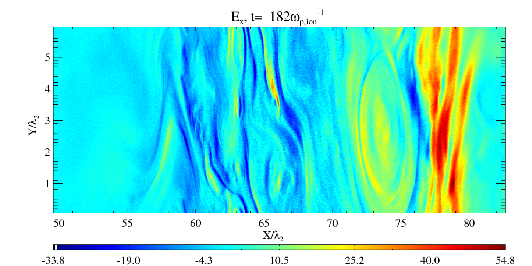
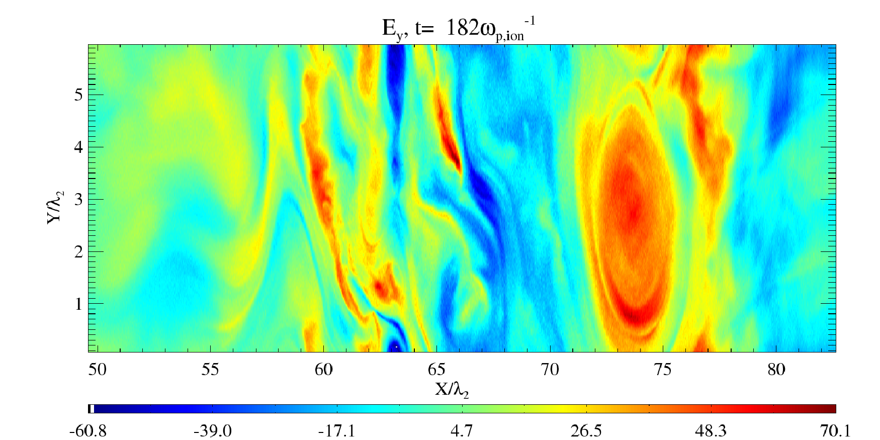
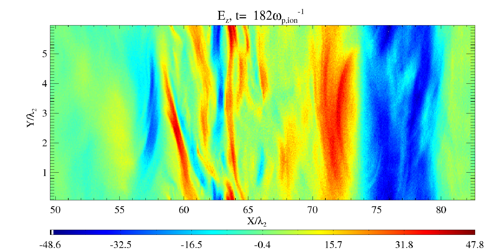
Figure 15: Electric field components at the time T2: Zoom of a 2D linear colorscale plot of the spatial distribution of $E_{x}$ (upper panel), $E_{y}$ (middle panel) and $E_{z}$ (lower panel).

The electric field amplitude is well below that of the magnetic field. Those of $E_{x}$ and $E_{y}$ are about half that of their magnetic counterparts, while that of $E_{z}$ amounts to a third of $B_{z}$. The electric energy density will thus be about 20% of the magnetic one.

Movie 3 shows a zoom of the time evolution of all six components of the electric and magnetic fields. We note that no signal, either wave or plasma structure, can be seen entering the simulation box on the left or right x-boundaries. In the lower four panels, $E_{y},E_{z}$ are clearly seen to be in phase and antiphase, respectively with the $B_{z},B_{y}$ components. Initially a strong dipolar field dominates, and filaments are clearly visible in the $E_{y},B_{z}$ components. The components parallel to the shock normal ($B_{x},E_{x}$) are considerably more fragmented than their perpendicular counterparts.

3.3 Generation of Mid-Infrared Synchrotron emission

The relativistic electrons are expected to emit synchrotron emission in the presence of a magnetic field. The synchrotron roll-off frequency is at $\nu_{rolloff}=\omega_{c}\gamma^{2}$, where $\omega_{c}$ is the electron cyclotron frequency. In the simulation we have found that for a mass ratio of $R=250$ the electrons are accelerated to Lorentz factors of $\sim 200$. We may assume from a comparison of the 1D PIC simulations with a mass ratio 100 and 400 in Refs. Bessho & Ohsawa (1999) and Dieckmann et al. (2008) that the peak electron Lorentz factor is proportional to the mass ratio. In this case and for a full mass ratio many electrons would reach Lorentz factors of 1500, this gives $1500^{2}\omega_{c}$. The magnetic field strength within a GRB jet is unknown and we have to resort to a guess. For an $\omega_{c}=\omega_{p,electron}=10^{5}$Hz this gives $\approx$ 200 GHz in the rest frame of the jet. There is a relativistic Doppler shift ($\delta=\sqrt{(1+\beta)/(1-\beta)}$) from the moving frame in the jet into the observer’s (Earth) frame. Assuming a $\beta=0.99999$ for GRB jets, giving $\delta=$ 450, we derive a frequency of 100 THz in the infrared frequency range. Secondary processes such as inverse Compton scattering from the population of $\Gamma\sim 400$ electrons are expected to upscatter the photons to gamma ray energies.

4 Discussion

In this paper we have examined the collision of two plasma clouds at a shock speed of 0.9c. The aim of the study is to gain insight into the behaviour of mildly relativistic shocks, and the associated phenomena of electron acceleration, magnetic field amplification, filament formation. The shock speed is at the lower end of the interval proposed for internal GRB shocks (Piran 1999). We add a quasi-parallel guiding magnetic field to the simulation, in order to probe the effects of a strong magnetization expected to be present. The mass ratio has been reduced to 250 to make the simulation more computationally tractable, while retaining the physical mass asymmetry which ensures a reservoir of ion energy is available to contribute to particle acceleration (Amato & Arons 2006). The density ratio of 10 has been chosen to emphasize the effects of asymmetry in GRB shocks. This paper extends MDD discussing in more detail the conditions that result in vortex formation also examining the electromagnetic field distribution at the shock front. While MDD only considered the currents, in this paper we focus on the particle acceleration mechanisms, not covered in the previous publication.

The magnetized background together with the colliding clouds ensures a jump in the convection electric field will be present. The initial jump in the convection electric field triggers the growth of a ramp in the magnetic field from which particles can be accelerated. This electromagnetic reaction to the plasma cloud collision is the first and most rapid response by the system. This ramp is initially planar as found by Dieckmann et al. (2010), but later evolves through plasma instabilities into a non-planar structure. Previous studies have shown that magnetized shocks have little particle acceleration unless ions are present (Hoshino et al. 1992; Amato & Arons 2006). Equally studies of weakly magnetized collisions have shown little or no difference to unmagnetized plasma (Nishikawa et al. 2003). The simultaneous presence of ions and of a strong guiding magnetic field show the rapid formation of a shock, which accelerates electrons to highly relativistic speeds and amplifies substantially the initial magnetic field.

The results shown here - in the context of the observations of polarisation in GRBs (Coburn & Boggs 2003; Steele et al. 2009) provide a compelling argument for the role of a dynamically significant primordial magnetic field from the jet. Such fields, in oblique collisions, provide a mechanism to transfer energy down the mass scales from ions to electrons, allowing electrons to increase their relativistic mass until they can be injected into the Fermi acceleration mechanism.

Based on the linear dispersion relation, we hypothesise that the filamentation instability is not suppressed in this regime of parameter space. The nonlinear simulation supports this hypothesis, but goes further to demonstrate a possible solution to the longstanding problem of filament lifetimes. Evidence for vortex formation is found, possibly a stable solution to offset rapid filament decay mechanisms (Waxman 2006). Such vortices are observed in nonrelativistic plasma flows (Alexandrova et al. 2006) and may thus not be unlikely structures in the more energetic astrophysical flows. The oblique shock considered here, also not unlikely in the context of GRB jets with helical background fields, allows sufficient transverse motion and transverse currents for a stable vortex structure to form through secondary instabilities. The simulation study reveals that the vortex has an internal structure akin to that of the cross-section of a flux tube that can be twisted into a spheromak in a 3D geometry (see MDD). The flux tube structure has a large inertia and is bound together by magnetic tension, possibly making it more resistant to dissipation on kinetic scales than the smaller-scale current filaments. During the simulation the flux tube continuously gains mass and magnetic field until its further growth is limited by the periodic boundary conditions along the shock boundary.

Comparing our work with the earlier 1D simulations by Bessho & Ohsawa (1999) and the 1D and 2D simulations (Dieckmann et al. 2008, 2010), we find that the near-equipartition energy acceleration predicted by these authors is confirmed. Martins et al. (2009) in their 2D piston simulations found that the upstream ions ahead of the shock were filamented, extending the region of magnetic field growth. We find that the magnetic field growth is exponential in the foreshock region.

Dieckmann et al. (2010) showed that the structures for a lower speed simulation and smaller magnetic-field-to-shock-normal angle are planar and 1D. The simulations presented here show a greater departure from one-dimensional behaviour. The greater field angle and flow speed in our work allows more motion transverse to the shock plane, which apparently triggers different processes in the shock transition layer.

The results shown here carry several important implications. Firstly, the filament generated magnetic field can be stored in magnetic vortices. We consider here a magnetic field that is relatively strong in that it yields an electron cyclotron frequency that is comparable to the electron plasma frequency. Secondly, oblique shocks have good acceleration properties, increasing electrons to near equipartition with ions. Thirdly, primordial fields are becoming increasingly accepted in GRBs and will have a decisive affect on the dynamics of plasma internal shock, acceleration of electrons and their injection into the Fermi mechanism. Fourthly, as is becoming evident (Lemoine & Pelletier 2010; Bret & Dieckmann 2010) a reduced mass ratio has an important effect on the results of PIC simulations and this approximation needs to be validated by linear theory if used. More specifically in the context considered here, heavier ions can undermine the magnetic suppression of the filamentation instability that may work for ions with a low mass.

Radiative losses can be non-negligible for shocked collisionless plasmas (Fleishman & Toptygin 2007; Schlickeiser & Lerche 2007, 2008). Although the PIC framework does not take into account radiative processes, we can infer that at least the radiative cooling by synchrotron-type emissions should not affect the conclusions propounded in this paper. The ions do not radiate significant energy and only a fraction of the electrons will convert some energy to low-energy photons through synchrotron cooling, in particular because the individual particles only spend a short amount of time in the high magnetic field region. The interaction between the relativistic electrons and the photon seed that is not captured by PIC simulations may, however, result in stronger energy losses.