Massless correlators of vector, scalar and tensor currents in position space at orders $\alpha_{s}^{3}$ and $\alpha_{s}^{4}$ : explicit analytical results

Abstract

We present analytical results both in momentum and position space for the massless correlators of the vector and scalar currents to order $\alpha_{s}^{4}$ as well as for the tensor currents to order $\alpha_{s}^{3}$. The evolution equations for the correlators together with all relevant anomalous dimensions are discussed in detail. As an application we present explicit conversion formulas relating the $\overline{\text{MS}}$-renormalized vector, scalar and tensor currents to their counterparts renormalized in the X-space renormalization scheme more appropriate for lattice calculations.

, ,

1 Introduction

Correlators of gauge invariant quark currents are important objects in QCD. It is enough to mention that the correlator of two vector currents is directly related to the famous ratio $R(s)={\sigma(e^{+}e^{-}\to{\rm hadrons})\over\sigma(e^{+}e^{-}\to\mu^{+}\mu^{-})}\,$, the Adler function and the decay widths of the Z-boson and the $\tau$-lepton (for a review see, e.g. [1]).

To be specific, let us consider a correlator:

$$\Pi(q)=i\int\text{d}x\ e^{iqx}\langle Tj(x)j^{\dagger}(0)\rangle{},$$ (1)

with $j$ being a gauge invariant local operator. The polarization operator $\Pi(q)$ satisfies the standard dispersion relation

$$\Pi(q)=\int_{0}^{\infty}\text{d}s\frac{\rho(s)}{s-q^{2}}-\mbox{subtractions}{},$$ (2)

The subtractions on the right-hand side of Eq. (2) are necessary as they remove an additional divergence coming from the vicinity of the region $x\sim 0$ in the $x$-integration in (1). The structure of the correlator (1) is significantly simplified if the momentum $q$ is considered as large compared to (active) quark masses. Setting then all quark masses to zero one can describe the general structure of the correlator in pQCD as follows:

$$\Pi(q)=(Q^{2})^{d-2}\sum_{i=1}^{\infty}\sum_{i\geq k\geq 0}\Pi_{ik}\,a_{s}^{i-1}(\mu)\,\left(\ln\frac{\mu^{2}}{Q^{2}}\right)^{k}{}.$$

Here $Q^{2}\equiv-q^{2}$, $a_{s}=\frac{\alpha_{s}}{\pi}$, $\mu$ stands for the renormalization scale and $d$ is the (mass) dimension of the current $j$.

In some applications it is useful to deal with the correlators in position space (see, e.g. [2, 3, 4, 5, 6] and below). Using a text-book formula for the massive scalar propagator in position space:

$$\Delta(x,s)\equiv\frac{1}{i(2\pi)^{4}}\int_{0}^{\infty}\text{d}q\,\frac{e^{iqx}}{s-q^{2}}=\frac{1}{-4\,\pi^{2}x^{2}}\,z\,K_{1}(z),\ \ z=\sqrt{-x^{2}\,s},$$ (3)

(with $K_{1}$ being a modified Bessel function) we arrive at a well-known representation for $\Pi$:

$$\Pi(x)=\int_{0}^{\infty}\text{d}s\,\Delta(x,s)\,\rho(s){}.$$ (4)

It should be stressed that the spectral density $\rho(s)$ does not depend on the non-logarithmical contributions to the sum in (1) (that is those proportional to the coefficients $\Pi_{ik}$ with $k\equiv 0$). Thus, the full correlator in position space considered as a function of $x$ (defined for all $x$ with $x^{2}\not=0$ ) also does not depend on non-logarithmical contributions to $\Pi(q)$.

In general, the operator $j$ is not scale-invariant (equivalently, has a non-zero anomalous dimension). The renormalization of the operator and the position space correlator look as follows

$$j=Z_{j}\,j_{0},\ \ \ \Pi(x)=Z^{2}_{j}\,\Pi_{0}(x){},$$ (5)

where $j_{0}$ and $\Pi_{0}$ stand for the corresponding bare quantities.

An important feature of the position space correlators is that they can be directly computed non-perturbatively on the lattice by Monte Carlo simulations (see, e.g. [7, 8, 9, 10]). Their long-distance behavior is governed by the non-perturbative features of the underlying field theory, QCD. On the other hand, due to asymptotic freedom, their short-distance behavior can be described by perturbation theory and operator product expansion (OPE). A meaningful comparison of perturbative results at short distances with their lattice counterparts requires, obviously, the use of one and the same renormalization prescription in the common case of scale-dependent operators. While minimal subtraction schemes ($\overline{\text{MS}}$ and its relatives [11, 12, 13]) are certainly preferable for perturbative calculations, they, clearly, can not be implemented on lattice.

A solution of the problem is based on the use of an intermediate renormalization scheme, with the renormalization conditions imposed directly on quark and gluon Green functions computed in a fixed gauge and for a particular configuration of external momenta [14].

A convenient intermediate scheme for the renormalization of the quark current operators has been developed in [9]. It is based on the study of the corresponding position space correlators and is called the X-space scheme. The conversion formulas between the $\overline{\text{MS}}$ and the X-space scheme have been elaborated in [9] to the next-to-leading order.

Recently there has been a lot of progress in computing higher order corrections to the vector and scalar correlators within perturbative QCD both in the massless limit as well as for the general case of massive quarks. Both correlators are now known in momentum space to order $\alpha_{s}^{3}$ [15, 16, 17, 18] (the real and absorptive parts) and even, partially, to order $\alpha_{s}^{4}$ [19, 20] (only the absorptive part in the massless limit). The situation is not so good for the tensor correlator, which is known completely to order $\alpha_{s}^{2}$ in the massless limit only [21].

In addition, the anomalous dimensions of the scalar and tensor currents are known to order $\alpha_{s}^{4}$ [22, 23, 24] (vector and axial-vector currents have identically vanishing anomalous dimension due to the corresponding Ward identity).

The aims of the present paper are:

• To compute the order $\alpha_{s}^{3}$ contribution to the tensor correlator (only absorptive part in the massless limit).

• To summarize available momentum space results for the scalar, vector and tensor (all massless) correlators and corresponding anomalous dimensions.

• To discuss in detail the evolution equations for all three correlators.

• To present full results for the correlators in position space, namely: scalar and vector to (and including) order $\alpha_{s}^{4}$ and tensor to (and including) order $\alpha_{s}^{3}$ computed within massless QCD.

• To construct the $N^{4}LO$ conversion formulas between $\overline{\text{MS}}$ and X-space renormalized scalar and vector currents as well as the $N^{3}LO$ ones for the tensor current.

• To study the stability of the conversion formulas with respect to higher order (not yet computed) perturbative corrections.

The plan of the paper is as follows. In the next section we discuss our conventions and the definition of the X-space renormalization scheme as well as a version of the $\overline{\text{MS}}$-scheme — the $\widetilde{\mbox{MS}}$-one which seems to be more convenient for renormalization of the position space correlators. Sections 3 and 4 list all available results for (massless) quark currents correlators in momentum and position space respectively. In Section 5 we try to provide the reader with the concise bibliographical information about the origin of the results collected in the two previous Sections as well as about the main technical tools employed in the corresponding calculations. Conversion formulas between the X-scheme and $\widetilde{\text{MS}}$/$\overline{\text{MS}}$ schemes are discussed in Section 6. In the last section 7 we summarize the content of the paper.

In addition, there are three appendixes. In Appendix A we spell out the rules which we use to construct the Euclidean correlator from its Minkowskian counterpart. Appendix B provides the reader with necessary information on the Fourier transformation. Appendix C lists various anomalous dimensions relevant for the RG evolution of the quark current correlators.

2 Quark current correlators in momentum and position space

In this section we outline our conventions and recall the definition of the X-space scheme as presented in Ref. [9]. Our discussion will focus on the correlator of scalar currents first. The generalization to other Lorentz structures is straightforward, we will comment on it towards the end of the section.

The scalar correlator in momentum space is defined as

$$\Pi^{S}(q)=i\int\text{d}x\ e^{iqx}\langle Tj(x)j(0)\rangle$$ (6)

with $j=\bar{\psi}\mathds{1}\psi$. For space-like momenta we can express the correlator in terms of the Euclidean momentum $Q$. In what follows we will work exclusively with Euclidean correlators. Our procedure of obtaining Euclidean correlators from Minkowskian ones is described in Appendix A. The correlator considered in position space reads

$$\Pi^{S}(X)=\langle j(X)j(0)\rangle$$ (7)

with a Euclidean separation $X$. We work in the chiral limit with $m_{\psi}=0$. Note that diagrams with purely gluonic cuts do not contribute to the scalar correlator (in the assumed massless limit) .

2.1 Momentum space

We denote the $\overline{\text{MS}}$ renormalized momentum space correlator at the scale $\mu$ by

$$\Pi^{S}(Q,\mu)=(Z^{S})^{2}\Pi_{0}^{S}(Q)+Z^{SS}(\mu^{2})^{-\epsilon}Q^{2}\,,$$ (8)

where $\Pi_{0}^{S}(Q)$ is the bare scalar correlator. Note that in addition to the multiplicative renormalization with $Z^{S}$ there is a subtractive counterterm $Z^{SS}$. The corresponding renormalization group equation reads

$$\mu^{2}\frac{\text{d}}{\text{d}\mu^{2}}\Pi^{S}(Q,\mu)=2\gamma^{S}\Pi^{S}(Q,\mu)+\gamma^{SS}Q^{2}$$ (9)

with the anomalous dimensions

$$\gamma^{S}=\mu^{2}\frac{\text{d}\log Z^{S}}{\text{d}\mu^{2}}\,,\qquad\gamma^{SS}=\mu^{2}\frac{\text{d}Z^{SS}}{\text{d}\mu^{2}}-(2\gamma^{S}+\epsilon)Z^{SS}\,.$$ (10)

Using the solution to the renormalization group equation (9), we can evolve the correlator from one scale $\mu_{0}$ to a different scale $\mu_{1}$:

$$\Pi^{S}(Q,\mu_{1})= \exp\left(\;\int\limits_{a_{s}(\mu_{0})}^{a_{s}(\mu_{1})}\frac{\text{d}z}{z}\frac{2\gamma^{S}(z)}{\beta(z)}\right)\big{(}\Pi^{S}(Q,\mu_{0})+Q^{2}\Delta(\mu_{1},\mu_{0})\big{)}\,,$$

$$\Delta(\mu_{1},\mu_{0})= \int\limits_{a_{s}(\mu_{0})}^{a_{s}(\mu_{1})}\frac{\text{d}z}{z}\frac{\gamma^{SS}(z)}{\beta(z)}\exp\left(-\int\limits^{z}_{a_{s}(\mu 0)}\frac{\text{d}z^{\prime}}{z^{\prime}}\frac{2\gamma^{S}(z^{\prime})}{\beta(z^{\prime})}\right)\,,$$ (11)

where $a_{s}=\alpha_{s}/\pi=g^{2}/(4\pi^{2})$, $g$ is the strong coupling constant and the $\beta$-function $\beta(a_{s})$ is defined as

$$\mu^{2}\frac{\text{d}}{\text{d}\mu^{2}}a_{s}=a_{s}\beta(a_{s})\equiv-\sum_{i\geq 0}\beta_{i}a_{s}^{i+2}{}.$$ (12)

While it is of course possible to recover logarithms explicitly using this solution, it is more convenient to rewrite the renormalization group equation into a differential equation in $l_{\mu Q}=\log(\mu^{2}/Q^{2})$ for this purpose:

$$\frac{\partial}{\partial l_{\mu Q}}\Pi^{S}(Q)=2\gamma^{S}\Pi^{S}(Q)+\gamma^{SS}Q^{2}-\beta\,a_{s}\frac{\partial}{\partial a_{s}}\Pi^{S}(Q)\,,$$ (13)

This equation can be used to iteratively reconstruct the logarithmic parts of $\Pi^{S}(Q)$. Explicit formulas for the anomalous dimensions and the QCD $\beta$ function are given in Appendix C.

2.2 Position space

In principle, the discussion of the preceding paragraph can be directly translated to the position space correlator. It is, however, convenient to use a modification of the MS scheme that is a bit different from the traditional $\overline{\text{MS}}$ convention. The reason for this is that in the $\overline{\text{MS}}$ scheme logarithms in position space naturally appear in the form

$$\log\left(\frac{\mu^{2}X^{2}}{4}\right)+2\*\gamma_{E}\,.$$ (14)

We can transform these to the simpler form $\log(\mu^{2}X^{2})$ with a shift in the renormalization scale:

$$\mu\to 2e^{-\gamma_{E}}\mu\approx 1.12\,\mu\,.$$ (15)

The shifted $\mu$ defines a new modified MS scheme which we call $\widetilde{\text{MS}}$. The relation between $\widetilde{\text{MS}}$ quantities and their $\overline{\text{MS}}$ counterparts is of course very simple:

$$\widetilde{\Pi}^{S}(X,\mu)=\Pi^{S}\Big{(}X,2e^{-\gamma_{E}}\mu\Big{)}\,,\qquad\widetilde{a}_{s}(\mu)=a_{s}\Big{(}2e^{-\gamma_{E}}\mu\Big{)}\,,$$ (16)

Using the evolution of the strong coupling constant we can also relate the $\widetilde{\text{MS}}$ coupling to the $\overline{\text{MS}}$ coupling at the same scale:

$$\begin{split}\tilde{a}_{s}(\mu)=&a_{s}(\mu)\bigg{\{}1-a_{s}(\mu)l\beta_{0}+a_{s}^{2}(\mu)l(\beta_{0}^{2}l-\beta_{1})+a_{s}^{3}(\mu)l\left(-\beta_{0}^{3}l^{2}+\frac{5}{2}\beta_{0}\beta_{1}l-\beta_{2}\right)\\ &+a_{s}^{4}(\mu)l\left[\beta_{0}^{4}l^{3}-\frac{13}{3}\beta_{0}^{2}\beta_{1}l^{2}+3\left(\frac{\beta_{1}^{2}}{2}+\beta_{0}\beta_{2}\right)l-\beta_{3}\right]+{\cal O}(a_{s}^{5}l^{5})\bigg{\}}\,,\end{split}$$ (17)

where $l=2\,(\log(2)-\gamma_{E})$.

In position space there is no additional subtractive renormalization. Hence, the renormalization group evolution simplifies to

$$\widetilde{\Pi}^{S}(X,\mu_{1})=\exp\left(\;\int\limits_{\tilde{a}_{s}(\mu_{0})}^{\tilde{a}_{s}(\mu_{1})}\frac{\text{d}z}{z}\frac{2\gamma^{S}(z)}{\beta(z)}\right)\tilde{\Pi}^{S}(X,\mu_{0})\,.$$ (18)

The evolution equation for the $\overline{\text{MS}}$ scheme is obtained from Eq. (18) by simply replacing $\widetilde{\text{MS}}$ quantities by their $\overline{\text{MS}}$ counterparts.

2.3 The X-space scheme

The X-space renormalization scheme is defined by fixing the correlator of the normalized current $j_{X}=Z^{S}_{X}j$ at a separation $X_{0}$ to its value in the free continuum theory [9]:

$$\Pi^{S}_{X}(X_{0})=(Z^{S}_{X})^{2}\,\Pi^{S}_{0}(X_{0})=\Pi^{S}(X_{0})\big{|}_{\text{free}}\,.$$ (19)

This prescription can be readily implemented both in lattice and perturbative QCD. In perturbation theory the free theory value of a correlator is obviously just the leading order contribution.

2.4 Other correlators

In addition to scalar correlators, we also consider correlators of vector, tensor, pseudo-scalar and axial-vector quark currents. In position space these are defined as

$$\Pi^{V}_{\mu\nu}(X)= \langle j_{\mu}(X)j_{\nu}(0)\rangle\,, \Pi^{T}_{\mu\nu\rho\sigma}(X)= \langle j_{\mu\nu}(X)j_{\rho\sigma}(0)\rangle\,,$$

$$\Pi^{P}(X)= \langle j_{5}(X)j_{5}(0)\rangle\,, \Pi^{A}_{\mu\nu}(X)= \langle j_{\mu 5}(X)j_{\nu 5}(0)\rangle$$ (20)

with

$$j_{5}=i\bar{\psi}\gamma_{5}\psi,\quad j_{\mu}=\bar{\psi}\gamma_{\mu}\psi,\quad j_{\mu 5}=\bar{\psi}\gamma_{\mu}\gamma_{5}\psi,\quad j_{\mu\nu}=\bar{\psi}\sigma_{\mu\nu}\psi\,.$$ (21)

Since we work with $m_{\psi}=0$, the results for the pseudo-scalar correlator will be the same as for the scalar correlator.

Except for two small points, the entire discussion for the scalar case also holds for the more complicated Lorentz structures. First, in contrast to all other correlators, the vector and the axial-vector correlators do receive contributions from diagrams with purely gluonic cuts. We choose to neglect them in this work. This implies that also vector- and axial-vector correlators coincide. Second, it is not possible to naïvely renormalise the vector correlator according to the X-space condition (Eq. (19)). The reason for this is that in position space its tensor structure varies between different orders of perturbation theory. We choose to renormalise the trace of the vector correlator instead.

3 Momentum space correlators: results

In the following two sections we present the results for the correlators both in momentum and position space. All results with their explicit renormalization scale dependence can also be retrieved from
http://www-ttp.particle.uni-karlsruhe.de/Progdata/ttp10/ttp10-42/

We list the correlators in momentum space at the scale $\mu^{2}=Q^{2}$, where all logarithms vanish. Results for arbitrary values of $\mu$ can be recovered by solving the renormalization group equation (i.e. by using Eq. (2.1) or (13)). Note that the anomalous dimensions listed in Appendix C allow the reconstruction of all logarithms at one order higher, i.e. at order $\alpha_{s}^{4}$ for the vector and scalar correlators and at order $\alpha_{s}^{3}$ for the tensor correlator.

$$\Pi^{S}(Q)=-\frac{3}{4\pi^{2}}\,\*Q^{2}\*\left(1+\sum_{n=1}^{\infty}C^{(n),s}a_{s}^{n}\right)\,,$$

$$C^{(1),s}=\frac{131}{24}-2\,\*\zeta_{3}\,,$$

$$C^{(2),s}=\frac{17645}{288}-\frac{353}{12}\*\zeta_{3}-\frac{1}{8}\*\zeta_{4}+\frac{25}{6}\*\zeta_{5}+n_{f}\*\Big{(}-\frac{511}{216}+\frac{2}{3}\*\zeta_{3}\Big{)}\,,$$

$$C^{(3),s}=\frac{215626549}{248832}-\frac{1789009}{3456}\*\zeta_{3}+\frac{1639}{32}\*\zeta_{3}^{2}-\frac{1645}{1152}\*\zeta_{4}+\frac{73565}{1728}\*\zeta_{5}$$

$$\phantom{C^{(3),s}=}+\frac{325}{192}\*\zeta_{6}-\frac{665}{72}\*\zeta_{7}+n_{f}\*\Big{(}-\frac{26364175}{373248}+\frac{22769}{864}\*\zeta_{3}-\frac{5}{6}\*\zeta_{3}^{2}-\frac{53}{48}\*\zeta_{4}$$

$$\phantom{C^{(3),s}=}+\frac{1889}{432}\*\zeta_{5}\Big{)}+n_{f}^{2}\*\Big{(}\frac{499069}{559872}-\frac{157}{1296}\*\zeta_{3}+\frac{1}{48}\*\zeta_{4}-\frac{5}{18}\*\zeta_{5}\Big{)}\,,$$ (22)

$$\Pi^{V}_{\mu\nu}(Q)=\frac{5}{12\pi^{2}}(-Q^{2}\delta_{\mu\nu}+Q_{\mu}Q_{\nu})\left(1+\sum_{n=1}^{\infty}C^{(n),v}a_{s}^{n}\right)\,,$$

$$C^{(1),v}=\frac{11}{4}-\frac{12}{5}\*\zeta_{3}\,,$$

$$C^{(2),v}=\frac{41927}{1440}-\frac{829}{30}\*\zeta_{3}+5\*\zeta_{5}+n_{f}\*\Big{(}-\frac{3701}{2160}+\frac{19}{15}\*\zeta_{3}\Big{)}\,,$$

$$C^{(3),v}=\frac{31431599}{69120}-\frac{624799}{1440}\*\zeta_{3}+\frac{99}{2}\*\zeta_{3}^{2}+\frac{11}{16}\*\zeta_{4}+\frac{349}{32}\*\zeta_{5}-\frac{133}{12}\*\zeta_{7}$$

$$\phantom{C^{(3),v}=}+n_{f}\*\Big{(}-\frac{1863319}{34560}+\frac{174421}{4320}\*\zeta_{3}-\zeta_{3}^{2}-\frac{11}{48}\*\zeta_{4}+\frac{109}{18}\*\zeta_{5}\Big{)}$$

$$\phantom{C^{(3),v}=}+n_{f}^{2}\*\Big{(}\frac{196513}{155520}-\frac{809}{1080}\*\zeta_{3}-\frac{1}{3}\*\zeta_{5}\Big{)}\,,$$ (23)

$$\Pi^{T}_{\mu\nu\rho\sigma}(Q)=Q^{2}\big{(}C^{t}\,T^{(1)}_{\mu\nu\rho\sigma}+D^{t}\,T^{(2)}_{\mu\nu\rho\sigma}(Q)\big{)}\,,$$

$$C^{t}=\frac{1}{12\pi^{2}}\Big{(}1+\sum_{n=1}^{\infty}C^{(n),t}a_{s}^{n}\Big{)}\,,\qquad D^{t}=-\frac{5}{12\pi^{2}}\Big{(}1+\sum_{n=1}^{\infty}D^{(n),t}a_{s}^{n}\Big{)}\,,$$

$$C^{(1),t}=\frac{491}{72}-6\*\zeta_{3}\,,$$

$$C^{(2),t}=\frac{556475}{7776}-\frac{2657}{36}\*\zeta_{3}+\frac{7}{24}\*\zeta_{4}+\frac{25}{2}\*\zeta_{5}+n_{f}\*\Big{(}-\frac{667}{162}+\frac{32}{9}\*\zeta_{3}\Big{)}\,,$$

$$D^{(1),t}=\frac{593}{180}-\frac{12}{5}\*\zeta_{3}\,,$$

$$D^{(2),t}=\frac{566777}{19440}-\frac{265}{9}\*\zeta_{3}+\frac{7}{60}\*\zeta_{4}+5\*\zeta_{5}+n_{f}\*\Big{(}-\frac{1333}{810}+\frac{64}{45}\*\zeta_{3}\Big{)}$$ (24)

with

$$a_{s}=\frac{\alpha_{s}\big{(}\sqrt{Q^{2}}\big{)}}{\pi}\,,\qquad\zeta_{n}=\sum_{k=1}^{\infty}\frac{1}{k^{n}}\,,$$

$$T^{(1)}_{\mu\nu\rho\sigma}=\delta_{\mu\rho}\delta_{\nu\sigma}-\delta_{\mu\sigma}\delta_{\nu\rho}\,,$$

$$T^{(2)}_{\mu\nu\rho\sigma}(Q)=\frac{Q_{\mu}Q_{\rho}}{Q^{2}}\delta_{\nu\sigma}-\frac{Q_{\mu}Q_{\sigma}}{Q^{2}}\delta_{\nu\rho}-\frac{Q_{\nu}Q_{\rho}}{Q^{2}}\delta_{\mu\sigma}+\frac{Q_{\nu}Q_{\sigma}}{Q^{2}}\delta_{\mu\rho}\,,$$ (25)

and $n_{f}$ active quark flavours.

4 Position space correlators: results

The position space results are obtained by four-dimensional Fourier transformation (see Appendix B) of their momentum space counterparts. As it was discussed in Section 1 the position space correlators are not sensitive (at $x^{2}\not=0$) to the constant (non-logarithmic) contributions to the momentum-space ones. Thus, the knowledge of the full vector and scalar momentum space correlators at order $\alpha_{s}^{3}$ plus the ${\cal O}(\alpha_{s}^{4})$ anomalous dimensions $\gamma^{SS}$ and $\gamma^{VV}$ from Appendix C allows us to present below the vector and scalar correlators in the position space at order $\alpha_{s}^{4}$. Similarly, the use of Eq. (13) and the ${\cal O}(\alpha_{s}^{3})$ anomalous dimensions $\gamma^{(1),TT}$ and $\gamma^{(2),TT}$ computed by us (see eqs. in Appendix C ) result to the full ${\cal O}(\alpha_{s}^{3})$ results for the position space tensor correlator.

We present the results in the $\widetilde{\text{MS}}$ scheme (see Eq. (16)) at the scale $\mu^{2}=\frac{1}{X^{2}}$ which correspond to $\overline{\text{MS}}$ results at the scale $\mu^{2}=\frac{4}{X^{2}}e^{-2\gamma_{E}}$. Results at an arbitrary scale $\mu$ can again be obtained with the use of the renormalization group evolution (Eq. (18)). The correlators in position space read

$$\widetilde{\Pi}^{S}(X)=\frac{3}{\pi^{4}\big{(}X^{2}\big{)}^{3}}\left(1+\sum_{n=1}^{\infty}\widetilde{C}^{(n),s}\tilde{a}_{s}^{n}\right)\,,$$

$$\widetilde{C}^{(1),s}=\frac{2}{3}\,,$$

$$\widetilde{C}^{(2),s}=\frac{817}{144}-\frac{39}{2}\*\zeta_{3}+n_{f}\*\Big{(}-\frac{23}{72}+\frac{2}{3}\*\zeta_{3}\Big{)}\,,$$

$$\widetilde{C}^{(3),s}=\frac{150353}{5184}-\frac{5125}{54}\*\zeta_{3}+\frac{815}{12}\*\zeta_{5}+n_{f}\*\Big{(}-\frac{13361}{3888}+\frac{3}{4}\*\zeta_{3}-\frac{5}{6}\*\zeta_{4}-\frac{25}{9}\*\zeta_{5}\Big{)}$$

$$\phantom{\widetilde{C}^{(3),s}=}+n_{f}^{2}\*\Big{(}-\frac{383}{11664}+\frac{8}{27}\*\zeta_{3}\Big{)}\,,$$

$$\widetilde{C}^{(4),s}=+\frac{22254833}{497664}-\frac{592067}{5184}\*\zeta_{3}+\frac{458425}{432}\*\zeta_{3}^{2}+\frac{265}{18}\*\zeta_{4}-\frac{607225}{864}\*\zeta_{5}$$

$$\phantom{\widetilde{C}^{(4),s}=}-\frac{1375}{32}\*\zeta_{6}-\frac{178045}{768}\*\zeta_{7}+n_{f}\*\Big{(}-\frac{8775605}{373248}-\frac{392129}{5184}\*\zeta_{3}$$

$$\phantom{\widetilde{C}^{(4),s}=}-\frac{955}{16}\*\zeta_{3}^{2}-\frac{6731}{576}\*\zeta_{4}+\frac{45695}{216}\*\zeta_{5}+\frac{2875}{288}\*\zeta_{6}+\frac{665}{72}\*\zeta_{7}\Big{)}$$

$$\phantom{\widetilde{C}^{(4),s}=}+n_{f}^{2}\*\Big{(}-\frac{224695}{2239488}+\frac{11263}{1296}\*\zeta_{3}+\frac{5}{6}\*\zeta_{3}^{2}+\frac{25}{96}\*\zeta_{4}-\frac{6515}{432}\*\zeta_{5}\Big{)}$$

$$\phantom{\widetilde{C}^{(4),s}=}+n_{f}^{3}\*\Big{(}\frac{6653}{559872}-\frac{173}{1296}\*\zeta_{3}+\frac{1}{144}\*\zeta_{4}+\frac{5}{18}\*\zeta_{5}\Big{)}\,,$$ (26)

$$\widetilde{\Pi}^{V}_{\mu\nu}(X)=\frac{6}{\pi^{4}\big{(}X^{2}\big{)}^{3}}\Bigg{[}\left(\frac{\delta_{\mu\nu}}{2}-\frac{X_{\mu}X_{\nu}}{X^{2}}\right)\*\widetilde{C}^{v}+\delta_{\mu\nu}\*\widetilde{D}^{v}\Bigg{]}\,,$$

$$\widetilde{C}^{v}=1+\sum_{n=1}^{\infty}\widetilde{C}^{(n),v}\tilde{a}_{s}^{n}\,,\qquad\widetilde{D}^{v}=\sum_{n=0}^{\infty}\widetilde{D}^{(n),v}\tilde{a}_{s}^{n}\,,$$

$$\widetilde{C}^{(1),v}=1\,,$$

$$\widetilde{C}^{(2),v}=\frac{61}{6}-11\*\zeta_{3}+n_{f}\*\Big{(}-\frac{11}{18}+\frac{2}{3}\*\zeta_{3}\Big{)}\,,$$

$$\widetilde{C}^{(3),v}=\frac{7309}{48}-\frac{989}{6}\*\zeta_{3}+\frac{275}{6}\*\zeta_{5}+n_{f}\*\Big{(}-\frac{2617}{144}+\frac{47}{3}\*\zeta_{3}-\frac{25}{9}\*\zeta_{5}\Big{)}$$

$$\phantom{\widetilde{C}^{(3),v}=}+n_{f}^{2}\*\Big{(}\frac{277}{648}-\frac{8}{27}\*\zeta_{3}\Big{)}\,,$$

$$\widetilde{C}^{(4),v}=\frac{57640705}{20736}-\frac{278401}{108}\*\zeta_{3}+\frac{5445}{8}\*\zeta_{3}^{2}-\frac{133705}{288}\*\zeta_{5}-\frac{7315}{48}\*\zeta_{7}$$

$$\phantom{\widetilde{C}^{(4),v}=}+n_{f}\*\Big{(}-\frac{10278875}{20736}+\frac{50705}{144}\*\zeta_{3}-55\*\zeta_{3}^{2}+\frac{65975}{432}\*\zeta_{5}+\frac{665}{72}\*\zeta_{7}\Big{)}$$

$$\phantom{\widetilde{C}^{(4),v}=}+n_{f}^{2}\*\Big{(}\frac{1554751}{62208}-\frac{10691}{864}\*\zeta_{3}+\frac{5}{6}\*\zeta_{3}^{2}-\frac{1315}{108}\*\zeta_{5}\Big{)}$$

$$\phantom{\widetilde{C}^{(4),v}=}+n_{f}^{3}\*\Big{(}-\frac{503}{1458}+\frac{2}{27}\*\zeta_{3}+\frac{5}{18}\*\zeta_{5}\Big{)}\,,$$

$$\widetilde{D}^{(0),v}=\widetilde{D}^{(1),v}=0\,,$$

$$\widetilde{D}^{(2),v}=-\frac{11}{24}+\frac{n_{f}}{36}\,,$$

$$\widetilde{D}^{(3),v}=-\frac{101}{9}+\frac{121}{12}\*\zeta_{3}+n_{f}\*\Big{(}\frac{587}{432}-\frac{11}{9}\*\zeta_{3}\Big{)}+n_{f}^{2}\*\Big{(}-\frac{1}{27}+\frac{1}{27}\*\zeta_{3}\Big{)}\,,$$

$$\widetilde{D}^{(4),v}=-\frac{616333}{2304}+\frac{1111}{4}\*\zeta_{3}-\frac{3025}{48}\*\zeta_{5}+n_{f}\*\Big{(}\frac{111409}{2304}-\frac{1607}{36}\*\zeta_{3}+\frac{275}{36}\*\zeta_{5}\Big{)}$$

$$\phantom{\widetilde{D}^{(4),v}=}+n_{f}^{2}\*\Big{(}-\frac{54373}{20736}+\frac{79}{36}\*\zeta_{3}-\frac{25}{108}\*\zeta_{5}\Big{)}+n_{f}^{3}\*\Big{(}\frac{325}{7776}-\frac{5}{162}\*\zeta_{3}\Big{)}\,,$$

$$\widetilde{\Pi}^{T}_{\mu\nu\rho\sigma}(X)=-\frac{6}{\pi^{4}\big{(}X^{2}\big{)}^{3}}\left(\frac{1}{2}T^{(1)}_{\mu\nu\rho\sigma}-T^{(2)}_{\mu\nu\rho\sigma}(X)\right)\left(1+\sum_{n=1}^{\infty}\widetilde{C}^{(n),t}\tilde{a}_{s}^{n}\right)\,,$$

$$\widetilde{C}^{(1),t}=2\,,$$

$$\widetilde{C}^{(2),t}=\frac{5303}{432}-\frac{143}{18}\*\zeta_{3}+n_{f}\*\Big{(}-\frac{443}{648}+\frac{2}{3}\*\zeta_{3}\Big{)}\,,$$

$$\widetilde{C}^{(3),t}=+\frac{8439437}{46656}-\frac{77977}{486}\*\zeta_{3}+\frac{29}{54}\*\zeta_{4}+\frac{2395}{108}\*\zeta_{5}$$

$$\phantom{\widetilde{C}^{(3),t}=}+n_{f}\*\Big{(}-\frac{246515}{11664}+\frac{1985}{108}\*\zeta_{3}+\frac{5}{18}\*\zeta_{4}-\frac{25}{9}\*\zeta_{5}\Big{)}$$

$$\phantom{\widetilde{C}^{(3),t}=}+n_{f}^{2}\*\Big{(}\frac{18287}{34992}-\frac{4}{9}\*\zeta_{3}\Big{)}\,,$$ (28)

with

$$\tilde{a}_{s}=\frac{\tilde{\alpha}_{s}\big{(}1/\sqrt{X^{2}}\big{)}}{\pi}\,,\qquad\zeta_{n}=\sum_{k=1}^{\infty}\frac{1}{k^{n}}\,,$$

$$T^{(1)}_{\mu\nu\rho\sigma}=\delta_{\mu\rho}\delta_{\nu\sigma}-\delta_{\mu\sigma}\delta_{\nu\rho}\,,$$

$$T^{(2)}_{\mu\nu\rho\sigma}(X)=\frac{X_{\mu}X_{\rho}}{X^{2}}\delta_{\nu\sigma}-\frac{X_{\mu}X_{\sigma}}{X^{2}}\delta_{\nu\rho}-\frac{X_{\nu}X_{\rho}}{X^{2}}\delta_{\mu\sigma}+\frac{X_{\nu}X_{\sigma}}{X^{2}}\delta_{\mu\rho}\,,$$ (29)

and $n_{f}$ active quark flavours.

In numerical form for $n_{f}=3$ the results read

$$\widetilde{\Pi}^{S}(X)=\frac{3}{\pi^{4}\big{(}X^{2}\big{)}^{3}}\big{(}1+0.67\,\tilde{a}_{s}-16.3\,\tilde{a}_{s}^{2}-31\,\tilde{a}_{s}^{3}+497\,\tilde{a}_{s}^{4}\big{)}\,,$$ (30)

$$\widetilde{\Pi}_{\mu\nu}^{V}(X)=\frac{6}{\pi^{4}\big{(}X^{2}\big{)}^{3}}\left(\frac{\delta_{\mu\nu}}{2}-\frac{X_{\mu}X_{\nu}}{X^{2}}\right)\big{(}1+\tilde{a}_{s}-2.5\,\tilde{a}_{s}^{2}-4.4\,\tilde{a}_{s}^{3}+66\,\tilde{a}_{s}^{4}\big{)}$$

$$\phantom{\widetilde{\Pi}_{\mu\nu}^{V}(X)=}-\delta_{\mu\nu}\big{(}-0.375\,\tilde{a}_{s}^{2}+0.63\,\tilde{a}_{s}^{3}+7.0\,\tilde{a}_{s}^{4}\big{)}\,,$$ (31)

$$\widetilde{\Pi}_{\mu\nu\rho\sigma}^{T}(X)=-\frac{6}{\pi^{4}\big{(}X^{2}\big{)}^{3}}\left(\frac{1}{2}T^{(1)}_{\mu\nu\rho\sigma}-T^{(2)}_{\mu\nu\rho\sigma}(X)\right)\big{(}1+2\,\tilde{a}_{s}+3.1\,\tilde{a}_{s}^{2}+6.6\,\tilde{a}_{s}^{3}\big{)}\,.$$ (32)

This can be compared to the $\overline{\text{MS}}$ results at the same scale $\mu^{2}=1/X^{2}$:

$$\Pi^{S}(X)=\frac{3}{\pi^{4}\big{(}X^{2}\big{)}^{3}}\big{(}1+0.20\,a_{s}-18.5\,a_{s}^{2}-11\,a_{s}^{3}+579\,a_{s}^{4}\big{)}\,,$$ (33)

$$\Pi_{\mu\nu}^{V}(X)=\frac{6}{\pi^{4}\big{(}X^{2}\big{)}^{3}}\left(\frac{\delta_{\mu\nu}}{2}-\frac{X_{\mu}X_{\nu}}{X^{2}}\right)\big{(}1+a_{s}-3.0\,a_{s}^{2}-2.4\,a_{s}^{3}+74\,a_{s}^{4}\big{)}$$

$$\phantom{\Pi_{\mu\nu}^{V}(X)=}-\delta_{\mu\nu}\big{(}-0.375\,a_{s}^{2}+1.0\,a_{s}^{3}+6.4\,a_{s}^{4}\big{)}\,,$$ (34)

$$\Pi_{\mu\nu\rho\sigma}^{T}(X)=-\frac{6}{\pi^{4}\big{(}X^{2}\big{)}^{3}}\left(\frac{1}{2}T^{(1)}_{\mu\nu\rho\sigma}-T^{(2)}_{\mu\nu\rho\sigma}(X)\right)\big{(}1.+2.15\,a_{s}+3.3\,a_{s}^{2}+6.4\,a_{s}^{3}\big{)}\,,$$ (35)

where we use the abbreviation $a_{s}=\alpha_{s}\big{(}1/\sqrt{X^{2}}\big{)}/\pi$. In both schemes the $\alpha_{s}^{4}$ coefficients of the vector and the scalar correlator are quite large. In the $\widetilde{\text{MS}}$ scheme we observe a slightly smaller $\alpha_{s}^{4}$ contribution; furthermore the coefficients are a bit more uniform between different orders. This indicates a better behavior of the perturbative series in this scheme.

It is remarkable that the Lorentz structure of the tensor correlator remains the same at each order while it begins to vary at order $\alpha_{s}^{2}$ in the vector correlator result. This change can be easily understood by considering the transversality condition

$$\partial_{\mu}\langle j_{\mu}(X)j_{\nu}(0)\rangle=0\,.$$ (36)

Together with the appearance of terms which are logarithmic in $X$ also the Lorentz structure has to change so that the vector correlator remains transversal (see Eq. (51) in Appendix B).

As a consequence of this, it is not possible to renormalise the vector correlator in the X-space scheme according to the prescription Eq. (19). There are many possible generalizations leading to a well-defined renormalization prescription for the vector correlator. Among them, we choose to renormalise the trace of the correlator. For the other correlators the renormalization is straightforward. We refrain from presenting the somewhat lengthy explicit results here. They can be easily constructed from the $\widetilde{\text{MS}}$ results (Eq. (4)-(4)) and the conversion formulas listed in Section 6 (Eq. (6)-(6)).

5 Bibliographical and technical comments

We start with some generic notes. First, the non-logarithmic part of a quark current correlator in momentum space is not physical within QCD as it requires additional UV subtractions beyond the ones associated to the coupling constant renormalization.

Still, the constant part is important because it provides us with a very convenient way to compute the $Q$-dependent (that is physical) contribution. Indeed, suppose that we want to get the $Q$-dependent contribution at order $\alpha_{s}^{n}$ to, say, the scalar correlator (the discussion below is general and applicable to every massless correlator). A direct calculation would require to deal with (n+1)-loop massless propagator-like diagrams contributing to $\Pi^{S}$. A better way is to use the evolution equation (13). Indeed, after a (trivial) integration of the right-hand side of the equation with respect to $l_{\mu Q}$ we arrive at the conclusion that the $Q$-dependent part of $\Pi^{S}$ is completely determined by the knowledge of three ingredients:

1. the very correlator $\Pi^{S}$ (including its constant, $Q$-independent part) and the beta-function to order $\alpha_{s}^{n}$ (both are contributed by $n$-loop diagrams);

2. the anomalous dimension $\gamma^{S}$ to order $\alpha_{s}^{n}$ ( $n$-loop diagrams);

3. the anomalous dimension $\gamma^{SS}$ to order $\alpha_{s}^{n+1}$ ($(n+1)$-loop diagrams).

	$\alpha_{s}^{2}$	$\alpha_{s}^{3}$	$\alpha_{s}^{4}$
$\Pi^{S}$	[17, 21], MINCER	[19, 26], $1/D$ expansion
$\gamma^{SS}$	[27, 17], MINCER	[17], MINCER, IRR	[19, 26], $1/D$ expansion,
			$R^{*}$-operation
$\text{Im}\,\Pi^{S}$	[27], MINCER	[17], MINCER, $R^{*}$-operation	[19], $1/D$ expansion,
			$R^{*}$-operation
$\Pi^{V}$	[15, 16, 21], MINCER	[20, 28], $1/D$ expansion
$\gamma^{VV}$	[25], MINCER	[15, 16], MINCER, IRR	[20, 28], $1/D$ expansion,
			$R^{*}$-operation
$\text{Im}\,\Pi^{V}$	[25], IRR	[17], MINCER, $R^{*}$-operation	[28], $1/D$ expansion,
			$R^{*}$-operation
$\Pi^{T}$	[21], MINCER
$\gamma^{TT}$	[21], MINCER	present work, MINCER, $R^{*}$-operation
$\text{Im}\,\Pi^{T}$	[21], MINCER	present work, MINCER, $R^{*}$-operation

Table 1: Calculations of massless quark correlators in QCD: references and main theoretical tools.

Moreover, it is a well-known fact that the methods of Infrared Rearrangements (IRR) [29] and $R^{*}$-operation [30] allow to reduce the problem of evaluation of a (n+1) loop contribution to an (arbitrary) anomalous dimension to the computation of some properly constructed set of n-loop massless propagator-like diagrams.

Up to and including three loops the massless propagator-like diagrams can be computed easily with the FORM [31] package MINCER [32, 33]. The package implements the algorithm developed in [34] and is based on the use of the traditional method of integration by parts. Another powerful approach — the method of the Gegenbauer Polynomials in x-space (GPTx) [13] — is less automated, but, sometimes, is applicable in cases with loop number exceeding three (see, e.g. [35] for recent spectacular examples).

The only systematical way to compute massless propagators at four loops is based on the so-called $1/D$-expansion elaborated in [36, 37] and on the use of a special parametric representation of Feynman integrals [38, 39, 40]. Here by computation we mean the reduction to the corresponding master integrals, the latter have been computed analytically [41] and numerically [42].

In Table 1 we display the bibliographic information about results listed in Sections 3,4, and in Appendix B. In addition we also mention the main theoretical tools used in obtaining these results.

We want also to stress, that literally all ${\cal O}(\alpha_{s}^{4})$ calculations listed in the Table would be not possible to perform without a heavy use of the parallel versions of FORM, PARFORM [43, 44, 45] and TFORM [46]. Last, but not least, the generation of thousands of four-and five-loop input QCD diagrams have been conveniently done with the help of the (FORTRAN) program QGRAF [47].

6 Conversion between X-space scheme and $\widetilde{\text{MS}}$ or $\overline{\text{MS}}$

The natural scale for a transition between the $\widetilde{\text{MS}}$ and the X-space scheme is

$$\tilde{\mu}_{0}^{2}=\frac{1}{X_{0}^{2}}\,.$$ (37)

This is obviously equivalent to a transition between $\overline{\text{MS}}$ and X-space scheme at a scale $\mu_{0}^{2}=\frac{4}{X_{0}^{2}}e^{-2\gamma_{E}}$. Imposing the X-space renormalization condition (Eq. (19)) on

$$\Pi^{\delta}_{X}(X_{0})=\left(\frac{Z^{\delta}_{X}}{\widetilde{Z}^{\delta}(\tilde{\mu}_{0})}\right)^{2}\widetilde{\Pi}^{\delta}(X_{0},\tilde{\mu}_{0})=\left(\frac{Z^{\delta}_{X}}{Z^{\delta}(\mu_{0})}\right)^{2}\Pi^{\delta}(X_{0},\mu_{0})$$ (38)

with $\delta\in\{V,\,S,\,T\}$ directly yields the desired ratios [9]

$$\frac{Z^{\delta}(\mu_{0})}{Z_{X}^{\delta}}=\frac{\widetilde{Z}^{\delta}(\tilde{\mu}_{0})}{Z_{X}^{\delta}}=\sqrt{\frac{\widetilde{\Pi}^{\delta}(X_{0},\tilde{\mu}_{0})}{\Pi^{\delta}(X_{0})\big{|}_{\text{free}}}}$$ (39)

between the renormalization constants in the different schemes. We obtain

$$\frac{\widetilde{Z}^{S}(\tilde{\mu}_{0})}{Z_{X}^{S}}=1+\sum_{n=1}^{\infty}\delta^{(n),s}\,\tilde{a}_{s}(\tilde{\mu}_{0})^{n}\,,$$

$$\delta^{(1),s}=\frac{1}{3}\,,$$

$$\delta^{(2),s}=\frac{89}{32}-\frac{39}{4}\*\zeta_{3}+n_{f}\*\Big{(}-\frac{23}{144}+\frac{1}{3}\*\zeta_{3}\Big{)}\,,$$

$$\delta^{(3),s}=\frac{140741}{10368}-\frac{2387}{54}\*\zeta_{3}+\frac{815}{24}\*\zeta_{5}+n_{f}\*\Big{(}-\frac{12947}{7776}+\frac{19}{72}\*\zeta_{3}-\frac{5}{12}\*\zeta_{4}-\frac{25}{18}\*\zeta_{5}\Big{)}$$

$$\phantom{\delta^{(3),s}=}+n_{f}^{2}\*\Big{(}-\frac{383}{23328}+\frac{4}{27}\*\zeta_{3}\Big{)}\,,$$

$$\delta^{(4),s}=\frac{13901515}{995328}-\frac{4393}{288}\*\zeta_{3}+\frac{208679}{432}\*\zeta_{3}^{2}+\frac{265}{36}\*\zeta_{4}-\frac{626785}{1728}\*\zeta_{5}$$

$$\phantom{\delta^{(4),s}=}-\frac{1375}{64}\*\zeta_{6}-\frac{178045}{1536}\*\zeta_{7}+n_{f}\*\Big{(}-\frac{8029687}{746496}-\frac{418799}{10368}\*\zeta_{3}$$

$$\phantom{\delta^{(4),s}=}-\frac{851}{32}\*\zeta_{3}^{2}-\frac{6571}{1152}\*\zeta_{4}+\frac{45895}{432}\*\zeta_{5}+\frac{2875}{576}\*\zeta_{6}+\frac{665}{144}\*\zeta_{7}\Big{)}$$

$$\phantom{\delta^{(4),s}=}+n_{f}^{2}\*\Big{(}-\frac{257315}{4478976}+\frac{11273}{2592}\*\zeta_{3}+\frac{13}{36}\*\zeta_{3}^{2}+\frac{25}{192}\*\zeta_{4}-\frac{6515}{864}\*\zeta_{5}\Big{)}$$

$$\phantom{\delta^{(4),s}=}+n_{f}^{3}\*\Big{(}\frac{6653}{1119744}-\frac{173}{2592}\*\zeta_{3}+\frac{1}{288}\*\zeta_{4}+\frac{5}{36}\*\zeta_{5}\Big{)}\,,$$ (40)

$$\frac{\widetilde{Z}^{V}(\tilde{\mu}_{0})}{Z_{X}^{V}}=(Z_{X}^{V})^{-1}=1+\sum_{n=1}^{\infty}\delta^{(n),v}\,\tilde{a}_{s}(\tilde{\mu}_{0})^{n}\,,$$

$$\delta^{(1),v}=\frac{1}{2}\,,$$

$$\delta^{(2),v}=\frac{97}{24}-\frac{11}{2}\*\zeta_{3}+n_{f}\*\Big{(}-\frac{1}{4}+\frac{1}{3}\*\zeta_{3}\Big{)}\,,$$

$$\delta^{(3),v}=\frac{14881}{288}-\frac{119}{2}\*\zeta_{3}+\frac{275}{12}\*\zeta_{5}+n_{f}\*\Big{(}-\frac{5395}{864}+\frac{47}{9}\*\zeta_{3}-\frac{25}{18}\*\zeta_{5}\Big{)}$$

$$\phantom{\delta^{(3),v}=}+n_{f}^{2}\*\Big{(}\frac{181}{1296}-\frac{2}{27}\*\zeta_{3}\Big{)}\,,$$

$$\delta^{(4),v}=\frac{34042561}{41472}-\frac{294371}{432}\*\zeta_{3}+\frac{5203}{16}\*\zeta_{3}^{2}-\frac{212905}{576}\*\zeta_{5}-\frac{7315}{96}\*\zeta_{7}$$

$$\phantom{\delta^{(4),v}=}+n_{f}\*\Big{(}-\frac{6096767}{41472}+\frac{7819}{96}\*\zeta_{3}-\frac{77}{3}\*\zeta_{3}^{2}+\frac{79775}{864}\*\zeta_{5}+\frac{665}{144}\*\zeta_{7}\Big{)}$$

$$\phantom{\delta^{(4),v}=}+n_{f}^{2}\*\Big{(}\frac{889699}{124416}-\frac{2899}{1728}\*\zeta_{3}+\frac{13}{36}\*\zeta_{3}^{2}-\frac{1415}{216}\*\zeta_{5}\Big{)}$$

$$\phantom{\delta^{(4),v}=}+n_{f}^{3}\*\Big{(}-\frac{1037}{11664}-\frac{2}{81}\*\zeta_{3}+\frac{5}{36}\*\zeta_{5}\Big{)}\,,$$ (41)

$$\frac{\widetilde{Z}^{T}(\tilde{\mu}_{0})}{Z_{X}^{T}}=1+\sum_{n=1}^{\infty}\delta^{(n),t}\,\tilde{a}_{s}(\tilde{\mu}_{0})^{n}\,,$$

$$\delta^{(1),t}=1\,,$$

$$\delta^{(2),t}=\frac{4871}{864}-\frac{143}{36}\*\zeta_{3}+n_{f}\*\Big{(}-\frac{443}{1296}+\frac{1}{3}\*\zeta_{3}\Big{)}\,,$$

$$\delta^{(3),t}=\frac{7913369}{93312}-\frac{18529}{243}\*\zeta_{3}+\frac{29}{108}\*\zeta_{4}+\frac{2395}{216}\*\zeta_{5}$$

$$\phantom{\delta^{(3),t}=}+n_{f}\*\Big{(}-\frac{238541}{23328}+\frac{1913}{216}\*\zeta_{3}+\frac{5}{36}\*\zeta_{4}-\frac{25}{18}\*\zeta_{5}\Big{)}+n_{f}^{2}\*\Big{(}\frac{18287}{69984}-\frac{2}{9}\*\zeta_{3}\Big{)}\,.$$ (42)

The conversion can of course be performed for an arbitrary scale $\mu$ with the help of the renormalization group evolution (Eq. (18)).

scalar correlator

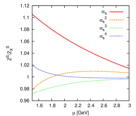
vector correlator

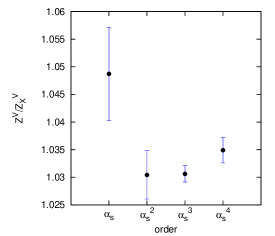
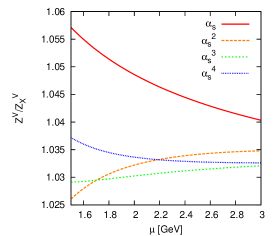
tensor correlator

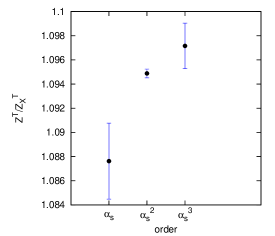
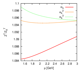
Figure 1: Values of $Z^{\delta}(2\,\text{GeV})/Z_{X}^{\delta}(X_{0}^{2})$ for vector, scalar and tensor currents with $X_{0}^{2}=(1.5\,\text{GeV})^{-2}$ and $n_{f}=3$ quark flavours at different orders in perturbation theory. The error bars on the left-hand side are obtained by running the ratio of renormalization constants from an intermediate scale $\mu$ with $1/X_{0}^{2}\leq\mu^{2}\leq 4/X_{0}^{2}$ to $2\,\text{GeV}$. On the right-hand side, the dependence on the choice of $\mu$ is shown.

scalar correlator

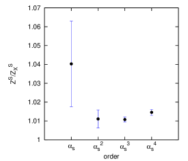
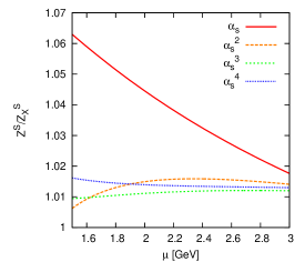
vector correlator

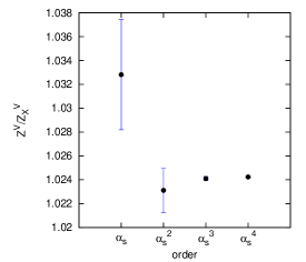
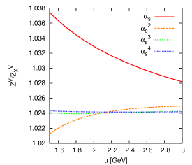
tensor correlator

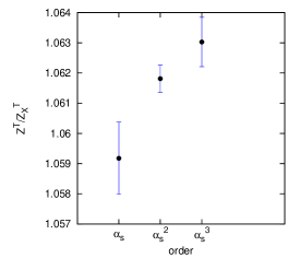
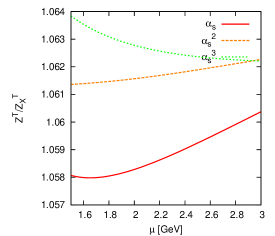
Figure 2: Values of $Z^{\delta}(2\,\text{GeV})/Z_{X}^{\delta}(X_{0}^{2})$ for vector, scalar and tensor currents with $X_{0}^{2}=(1.5\,\text{GeV})^{-2}$ and $n_{f}=0$ quark flavours at different orders in perturbation theory.

The new higher order results reduce the theoretical error significantly compared to the old NLO conversion formulas of Ref. [9]. As an example we show the values of $Z^{\delta}(2\,\text{GeV})/Z_{X}^{\delta}(X_{0}^{2})$ with $\delta\in\{V,\,S,\,T\}$, $X_{0}^{2}=(1.5\,\text{GeV})^{-2}$ at different orders in perturbation theory. We estimate the theory error from higher orders by performing the transition between the two schemes at some varying intermediate scale $\mu$ and evolving the result to the final scale of $2\,\text{GeV}$:

$$\frac{Z^{\delta}(2\,\text{GeV})}{Z_{X}^{\delta}(X_{0}^{2})}=\exp\left(\int\limits_{a_{s}(\mu)}^{a_{s}(2\,\text{GeV})}\frac{\text{d}z}{z}\frac{\gamma^{\delta}(z)}{\beta(z)}\right)\frac{Z^{\delta}(\mu)}{Z_{X}^{\delta}(X_{0}^{2})}\,.$$ (43)

For the evolution, we use anomalous dimensions at one order higher than $Z^{\delta}(2\,\text{GeV})/Z_{X}^{\delta}(X_{0}^{2})$, up to the highest available order of $\alpha_{s}^{4}$. In Figure 1 the values for this transition factor are plotted for a varying intermediate scale $\mu^{2}$ between $1/X_{0}^{2}$ and $4/X_{0}^{2}$ and $n_{f}=3$ quark flavours. Figure 2 shows the same ratios of renormalization constants for $n_{f}=0$. As expected from the numerical formulas Eqs. (33)-(35) the vector and scalar correlators receive large contributions at order $\alpha_{s}^{2}$ and $\alpha_{s}^{4}$ for $n_{f}=3$.

7 Conclusion

In this work we have presented presently available information on three basic quark currents correlators — the scalar, vector and the tensor ones — considered within the massless QCD. The correlators and the corresponding RG evolution equations have been studied both in the momentum and position space. Explicit conversion formulas relating the $\overline{\text{MS}}$ renormalized vector, scalar and tensor currents to their counterparts renormalized in the X-space renormalization scheme are constructed. It is demonstrated that the new higher order results reduce the theoretical error significantly compared to the old NLO conversion formulas of Ref. [9].

Appendix A Euclidean correlators from Minkowskian ones

Let us consider a generic correlator defined originally in the Minkowskian space:

$$\Pi_{{\mu_{1}\mu_{2}\dots}{\nu_{1}\nu_{2}\dots}}(q)= \,i\int_{M}\text{d}x\ e^{iqx}\langle Tj_{\nu_{1}\nu_{2}\dots}(x)\,\,j^{\dagger}_{\mu_{1}\mu_{2}\dots}(0)\rangle$$ (44)

$$= \,\sum_{k}T^{k}_{{\mu_{1}\mu_{2}\dots}(q){\nu_{1}\nu_{2}\dots}}(q)\,\Pi_{k}(-q^{2}){},$$ (45)

where the tensors $T^{k}_{{\mu_{1}\mu_{2}\dots}{\nu_{1}\nu_{2}\dots}}$ are made from the metric tensor $g_{\mu\nu}$, the vector $q$ and the indexes ${\mu_{1}\mu_{2}\dots}{\nu_{1}\nu_{2}\dots}$.

The corresponding Euclidean correlator in the momentum space is constructed as follows:

$$\Pi_{{\mu_{1}\mu_{2}\dots}{\nu_{1}\nu_{2}\dots}}(Q)\equiv\sum_{k}T^{k}_{{\mu_{1}\mu_{2}\dots}{\nu_{1}\nu_{2}\dots}}(Q)\,\,\Pi_{k}(Q^{2}){},$$ (46)

with $T^{k}_{{\mu_{1}\mu_{2}\dots}{\nu_{1}\nu_{2}\dots}}(Q)$ being made from $T^{k}_{{\mu_{1}\mu_{2}\dots}{\nu_{1}\nu_{2}\dots}}(q)$ with the help of the replacements $q_{\mu_{i}}\to-Q_{\mu_{i}},q_{\nu_{i}}\to-Q_{\nu_{i}},g_{\mu\nu}\to-\delta_{\mu\nu}$.

At last, the Euclidean correlator in the position space is defined with the help of the Fourier transformation, viz.

$$\Pi_{{\mu_{1}\mu_{2}\dots}{\nu_{1}\nu_{2}\dots}}(Q)\equiv\int_{E}\text{d}X\ e^{iQX}\langle Tj_{\nu_{1}\nu_{2}\dots}(X)\,\,j^{\dagger}_{\mu_{1}\mu_{2}\dots}(0)\rangle$$ (47)

Appendix B Fourier transformation in $\mathbf{d}$ dimensions

Perturbative calculations are in most cases quite cumbersome in position space. A more convenient alternative is to perform the calculation in momentum space, where exploiting invariance under translations (implying momentum conservation) leads to great simplifications. In the end, the result in position space can be recovered by means of Fourier transformation.

B.1 Fourier transformation of bare functions

In the current work, all bare Green functions have a power-like dependence on the momentum. For the transformation from euclidean momentum space to euclidean position space we use the following formula:

$$\operatorname{FT}\big{(}(Q^{2})^{-r}\big{)}\equiv\int\frac{\text{d}^{d}Q}{(2\pi)^{d}}\frac{e^{iQX}}{(Q^{2})^{r}}=\frac{1}{(4\pi)^{\frac{d}{2}}}\frac{\Gamma(\frac{d}{2}-r)}{\Gamma(r)}\left(\frac{X^{2}}{4}\right)^{r-\frac{d}{2}}\,.$$ (48)

It is straightforward to derive this formula by using Schwinger parametrization and Gauss integration.

For Green functions with a non-trivial Lorentz structure it is convenient to use momentum operators, i.e.

$$Q_{\mu}\to -i\frac{\partial}{\partial X_{\mu}}\,,$$ (49)

$$\operatorname{FT}\big{(}Q_{\mu}Q_{\nu}(Q^{2})^{-(r+1)}\big{)}= \frac{1}{(4\pi)^{\frac{d}{2}}}\frac{\Gamma(\frac{d}{2}-r)}{\Gamma(r)}\left(\frac{X^{2}}{4}\right)^{r-\frac{d}{2}}\left[\frac{\delta_{\mu\nu}}{2r}-\left(\frac{d}{2r}-1\right)\frac{X_{\mu}X_{\nu}}{X^{2}}\right]\,.$$ (50)

Note that forming the trace of the right-hand side of Eq. (50) again yields the simpler result from Eq. (48).

We also see explicitly that the Fourier transformation preserves transversality. Combining Eqs. (48) and (50) we obtain

$$\operatorname{FT}\left[\left(\delta_{\mu\nu}-\frac{Q_{\mu}Q_{\nu}}{Q^{2}}\right)(Q^{2})^{-r}\right]= \frac{1}{(4\pi)^{\frac{d}{2}}}\frac{\Gamma(\frac{d}{2}-r)}{\Gamma(r)}\left(\frac{X^{2}}{4}\right)^{r-\frac{d}{2}}$$ (51)

$$\quad\times\left[\left(1-\frac{1}{2r}\right)\delta_{\mu\nu}-\left(1-\frac{d}{2r}\right)\frac{X_{\mu}X_{\nu}}{X^{2}}\right]\,,$$

$$\partial_{\mu}\operatorname{FT}\left[\left(\delta_{\mu\nu}-\frac{Q_{\mu}Q_{\nu}}{Q^{2}}\right)(Q^{2})^{-r}\right]= \partial_{\nu}\operatorname{FT}\left[\left(\delta_{\mu\nu}-\frac{Q_{\mu}Q_{\nu}}{Q^{2}}\right)(Q^{2})^{-r}\right]=0\,.$$ (52)

B.2 Fourier transformation in four dimensions

The Fourier transformation for the correlators we consider is regular at $d=4$. This means that there are two ways of obtaining the renormalized correlators in position space. On the one hand, we can transform the bare Green functions in $d$ dimensions and perform the renormalization afterwards. On the other hand, we can start from the renormalized correlator in momentum space and transform it in four dimensions. In the latter case we have to transform terms which are logarithmic in $Q^{2}$ in addition to simple powers of $Q^{2}$. Rewriting the logarithms with the help of derivatives leads to

$$\operatorname{FT}\big{[}\left(Q^{2}\right)^{r}\log^{s}\left(Q^{2}\right)\big{]}=\lim_{\delta\to 0}\bigg{(}\frac{\partial}{\partial\delta}\bigg{)}^{s}\operatorname{FT}\big{[}\left(Q^{2}\right)^{r+\delta}\big{]}\,.$$ (53)

In Table 2 the resulting expressions are listed for all powers of $Q^{2}$ and $\log\left(Q^{2}\right)$ which appear in the momentum space correlators up to order $\alpha_{s}^{4}$.

Momentum space	Position space
$\log(\mu^{2}/Q^{2})$	$\frac{1}{\pi^{2}\*(X^{2})^{2}}$
$\log^{2}(\mu^{2}/Q^{2})$	$\frac{2}{\pi^{2}\*(X^{2})^{2}}\*(-1+l_{\mu X})$
$\log^{3}(\mu^{2}/Q^{2})$	$\frac{3}{\pi^{2}\*(X^{2})^{2}}\*(-2\*l_{\mu X}+l_{\mu X}^{2})$
$\log^{4}(\mu^{2}/Q^{2})$	$\frac{4}{\pi^{2}\*(X^{2})^{2}}\*(4\*\zeta_{3}-3\*l_{\mu X}^{2}+l_{\mu X}^{3})$
$\log^{5}(\mu^{2}/Q^{2})$	$\frac{5}{\pi^{2}\*(X^{2})^{2}}\*(-16\*\zeta_{3}+16\*l_{\mu X}\*\zeta_{3}-4\*l_{\mu X}^{3}+l_{\mu X}^{4})$
$Q^{2}\*\log(\mu^{2}/Q^{2})$	$-\frac{8}{\pi^{2}\*(X^{2})^{3}}$
$Q^{2}\*\log^{2}(\mu^{2}/Q^{2})$	$\frac{8}{\pi^{2}\*(X^{2})^{3}}\*(5-2\*l_{\mu X})$
$Q^{2}\*\log^{3}(\mu^{2}/Q^{2})$	$\frac{24}{\pi^{2}\*(X^{2})^{3}}\*(-4+5\*l_{\mu X}-l_{\mu X}^{2})$
$Q^{2}\*\log^{4}(\mu^{2}/Q^{2})$	$\frac{16}{\pi^{2}\*(X^{2})^{3}}\*(6-8\*\zeta_{3}-24\*l_{\mu X}+15\*l_{\mu X}^{2}-2\*l_{\mu X}^{3})$
$Q^{2}\*\log^{5}(\mu^{2}/Q^{2})$	$\frac{40}{\pi^{2}\*(X^{2})^{3}}\*(40\*\zeta_{3}+12\*l_{\mu X}-16\*l_{\mu X}\*\zeta_{3}-24\*l_{\mu X}^{2}+10\*l_{\mu X}^{3}-l_{\mu X}^{4})$

Table 2: Fourier transformation of logarithmic terms for various powers of $Q^{2}$ and $\log Q^{2}$. Terms that do not contain logarithms vanish for non-negative integer powers of $Q^{2}$. We use the abbreviation $l_{\mu X}=\log(\mu^{2}X^{2}/4)+2\gamma_{E}$.

B.3 Logarithmic structure

One-scale problems, like the correlators considered in this work, exhibit a very special structure of their logarithmic terms both in momentum and in position space.

In momentum space in the $\overline{\text{MS}}$ scheme, logarithms have the form $\log(\mu^{2}/Q^{2})$. They originate from terms of the form

$$\left(\frac{\mu^{2}}{Q^{2}}\right)^{l\epsilon}=1+l\epsilon\log\left(\frac{\mu^{2}}{Q^{2}}\right)+{\cal O}\big{(}\epsilon^{2}\big{)}\,,$$ (54)

where $l$ denotes the number of loops in the corresponding diagram. In order to obtain the logarithmic structure in position space we can again extract terms of the form $y^{l\epsilon}$ from the Fourier transform of the left-hand side of Eq. (54). Expressing the Gamma functions in the Fourier transform in terms of exponential functions and polynomials in $\epsilon$ we find

$$\left(\frac{\mu^{2}X^{2}}{4}e^{2\gamma_{E}}\right)^{l\epsilon}=1+l\epsilon\Bigg{[}\log\left(\frac{\mu^{2}X^{2}}{4}\right)+2\gamma_{E}\Bigg{]}+{\cal O}\big{(}\epsilon^{2}\big{)}\,,$$ (55)

for the general structure of position space logarithms.

Appendix C Anomalous dimensions

In our conventions the momentum space renormalization group equations of the scalar, vector and tensor correlators read

$$\mu^{2}\frac{\text{d}}{\text{d}\mu^{2}}\Pi^{S}(Q,\mu)=2\gamma^{S}\Pi^{S}(Q,\mu)+\gamma^{SS}Q^{2}\,,$$ (56)

$$\mu^{2}\frac{\text{d}}{\text{d}\mu^{2}}\Pi^{V}_{\mu\nu}(Q,\mu)=2\gamma^{V}\Pi^{V}_{\mu\nu}(Q,\mu)+\gamma^{VV}(-Q^{2}\delta_{\mu\nu}+Q_{\mu}Q_{\nu})\,,$$ (57)

$$\mu^{2}\frac{\text{d}}{\text{d}\mu^{2}}\Pi^{T}_{\mu\nu\rho\sigma}(Q,\mu)=2\gamma^{T}\Pi^{T}_{\mu\nu\rho\sigma}(Q,\mu)+\big{(}\gamma^{(1),TT}T^{(1)}_{\mu\nu\rho\sigma}+\gamma^{(2),TT}T^{(2)}_{\mu\nu\rho\sigma}(Q)\big{)}Q^{2}$$ (58)

with the tensor structures

$$T^{(1)}_{\mu\nu\rho\sigma}=\delta_{\mu\rho}\delta_{\nu\sigma}-\delta_{\mu\sigma}\delta_{\nu\rho}\,,$$

$$T^{(2)}_{\mu\nu\rho\sigma}(Q)=\frac{Q_{\mu}Q_{\rho}}{Q^{2}}\delta_{\nu\sigma}-\frac{Q_{\mu}Q_{\sigma}}{Q^{2}}\delta_{\nu\rho}-\frac{Q_{\nu}Q_{\rho}}{Q^{2}}\delta_{\mu\sigma}+\frac{Q_{\nu}Q_{\sigma}}{Q^{2}}\delta_{\mu\rho}\,.$$ (59)

The corresponding evolution equations in position space are analogous, but contain no subtractive anomalous dimensions. The anomalous dimensions are given by

$$\gamma^{V}(a_{s})=\,0\,,$$ (60)

$$\gamma^{VV}(a_{s})=\frac{1}{16\pi^{2}}\sum_{n=0}^{\infty}\gamma^{VV}_{n}a_{s}^{n}\,,$$

$$\gamma^{VV}_{0}=4\,,$$

$$\gamma^{VV}_{1}=4\,,$$

$$\gamma^{VV}_{2}=\frac{125}{12}-\frac{11}{18}n_{f}\,,$$

$$\gamma^{VV}_{3}=\frac{10487}{432}+\frac{110}{9}\zeta_{3}+n_{f}\Big{(}-\frac{707}{216}-\frac{110}{27}\,\zeta_{3}\Big{)}-\frac{77}{972}n_{f}^{2}\,,$$

$$\gamma^{VV}_{4}=\frac{2665349}{41472}+\frac{182335}{864}\zeta_{3}-\frac{605}{16}\zeta_{4}-\frac{31375}{288}\zeta_{5}$$

$$\phantom{\gamma^{VV}_{4}=}+n_{f}\Big{(}-\frac{11785}{648}-\frac{58625}{864}\zeta_{3}+\frac{715}{48}\zeta_{4}+\frac{13325}{432}\zeta_{5}\Big{)}$$

$$\phantom{\gamma^{VV}_{4}=}+n_{f}^{2}\Big{(}-\frac{4729}{31104}+\frac{3163}{1296}\zeta_{3}-\frac{55}{72}\zeta_{4}\Big{)}+n_{f}^{3}\Big{(}\frac{107}{15552}+\frac{1}{108}\zeta_{3}\Big{)}\,,$$ (61)

$$\gamma^{S}(a_{s})=-\gamma_{m}=\sum_{n=0}^{\infty}\gamma^{S}_{n}a_{s}^{n+1}\,,$$

$$\gamma^{S}_{0}=1\,,$$

$$\gamma^{S}_{1}=\frac{101}{24}-\frac{5}{36}\*n_{f}\,,$$

$$\gamma^{S}_{2}=\frac{1249}{64}+n_{f}\*\Big{(}-\frac{277}{216}-\frac{5}{6}\*\zeta_{3}\Big{)}-\frac{35}{1296}\*n_{f}^{2}\,,$$

$$\gamma^{S}_{3}=\frac{4603055}{41472}+\frac{530}{27}\*\zeta_{3}-\frac{275}{8}\*\zeta_{5}+n_{f}\*\Big{(}-\frac{91723}{6912}-\frac{2137}{144}\*\zeta_{3}+\frac{55}{16}\*\zeta_{4}+\frac{575}{72}\*\zeta_{5}\Big{)}$$

$$\phantom{\gamma^{S}_{3}=}+n_{f}^{2}\*\Big{(}\frac{2621}{31104}+\frac{25}{72}\*\zeta_{3}-\frac{5}{24}\*\zeta_{4}\Big{)}+n_{f}^{3}\*\Big{(}-\frac{83}{15552}+\frac{1}{108}\*\zeta_{3}\Big{)}\,,$$ (62)

$$\gamma^{SS}(a_{s})=\frac{1}{16\pi^{2}}\sum_{n=0}^{\infty}\gamma^{SS}_{n}a_{s}^{n}\,,$$

$$\gamma^{SS}_{0}=-6\,,$$

$$\gamma^{SS}_{1}=-10\,,$$

$$\gamma^{SS}_{2}=-\frac{455}{12}+3\*\zeta_{3}-2\,n_{f}\,,$$

$$\gamma^{SS}_{3}=-\frac{157697}{864}+\frac{1645}{36}\*\zeta_{3}-\frac{45}{4}\*\zeta_{4}-\frac{65}{2}\*\zeta_{5}+n_{f}\*\Big{(}\frac{14131}{1296}+\frac{26}{3}\*\zeta_{3}+\frac{11}{2}\*\zeta_{4}\Big{)}$$

$$\phantom{\gamma^{SS}_{3}=}+n_{f}^{2}\*\Big{(}\frac{1625}{1944}-\frac{2}{3}\*\zeta_{3}\Big{)}\,,$$

$$\gamma^{SS}_{4}=-\frac{1305623}{864}-\frac{540883}{3456}\*\zeta_{3}-\frac{19327}{288}\*\zeta_{3}^{2}-\frac{113557}{384}\*\zeta_{4}+\frac{158765}{576}\*\zeta_{5}+\frac{29825}{64}\*\zeta_{6}$$

$$\phantom{\gamma^{SS}_{4}=}+\frac{97895}{384}\*\zeta_{7}+n_{f}\*\Big{(}\frac{11341807}{62208}+\frac{385147}{1728}\*\zeta_{3}-\frac{187}{16}\*\zeta_{3}^{2}+\frac{10207}{192}\*\zeta_{4}$$

$$\phantom{\gamma^{SS}_{4}=}-\frac{55127}{288}\*\zeta_{5}-\frac{6725}{96}\*\zeta_{6}\Big{)}+n_{f}^{2}\*\Big{(}\frac{249113}{373248}-\frac{749}{48}\*\zeta_{3}+\frac{21}{8}\*\zeta_{4}+\frac{37}{4}\*\zeta_{5}\Big{)}$$

$$\phantom{\gamma^{SS}_{4}=}+n_{f}^{3}\*\Big{(}\frac{1625}{15552}+\frac{5}{108}\*\zeta_{3}-\frac{1}{6}\*\zeta_{4}\Big{)}\,,$$ (63)

$$\gamma^{T}(a_{s})=\sum_{n=0}^{\infty}\gamma^{T}_{n}a_{s}^{n+1}\,,$$

$$\gamma^{T}_{0}=-\frac{1}{3}\,,$$

$$\gamma^{T}_{1}=-\frac{181}{72}+\frac{13}{108}\*n_{f}\,,$$

$$\gamma^{T}_{2}=-\frac{52555}{5184}+\frac{29}{54}\*\zeta_{3}+n_{f}\*\Big{(}\frac{655}{648}+\frac{5}{18}\*\zeta_{3}\Big{)}+\frac{n_{f}^{2}}{144}\,,$$

$$\gamma^{T}_{3}=-\frac{2208517}{41472}+\frac{7733}{3888}\*\zeta_{3}-\frac{319}{144}\*\zeta_{4}+\frac{10465}{972}\*\zeta_{5}$$

$$\phantom{\gamma^{T}_{3}=}+n_{f}\*\Big{(}\frac{1537379}{186624}+\frac{18979}{3888}\*\zeta_{3}-\frac{437}{432}\*\zeta_{4}-\frac{575}{216}\*\zeta_{5}\Big{)}$$

$$\phantom{\gamma^{T}_{3}=}+n_{f}^{2}\*\Big{(}-\frac{9961}{93312}-\frac{115}{648}\*\zeta_{3}+\frac{5}{72}\*\zeta_{4}\Big{)}+n_{f}^{3}\*\Big{(}-\frac{7}{15552}-\frac{1}{324}\*\zeta_{3}\Big{)}\,,$$ (64)

$$\gamma^{(1),TT}(a_{s})=\frac{1}{16\pi^{2}}\sum_{n=0}^{\infty}\gamma^{(1),TT}_{n}a_{s}^{n}\,,$$

$$\gamma^{(1),TT}_{0}=2\,,$$

$$\gamma^{(1),TT}_{1}=\frac{22}{9}\,,$$

$$\gamma^{(1),TT}_{2}=\frac{841}{324}+\frac{7}{9}\*\zeta_{3}+\frac{n_{f}}{81}\,,$$

$$\gamma^{(1),TT}_{3}=\frac{617299}{69984}+\frac{35171}{972}\*\zeta_{3}-\frac{29}{36}\*\zeta_{4}-\frac{1955}{54}\*\zeta_{5}$$

$$\phantom{\gamma^{(1),TT}_{3}=}+n_{f}\*\Big{(}\frac{32821}{34992}-\frac{152}{81}\*\zeta_{3}+\frac{37}{54}\*\zeta_{4}\Big{)}+n_{f}^{2}\*\Big{(}\frac{557}{17496}-\frac{2}{27}\*\zeta_{3}\Big{)}\,,$$ (65)

$$\gamma^{(2),TT}(a_{s})=\frac{1}{16\pi^{2}}\sum_{n=0}^{\infty}\gamma^{(2),TT}_{n}a_{s}^{n}\,,$$

$$\gamma^{(2),TT}_{0}=-4\,,$$

$$\gamma^{(2),TT}_{1}=-\frac{68}{9}\,,$$

$$\gamma^{(2),TT}_{2}=-\frac{1412}{81}-\frac{14}{9}\*\zeta_{3}+\frac{25}{81}\*n_{f}\,,$$

$$\gamma^{(2),TT}_{3}=-\frac{2679661}{34992}-\frac{31865}{486}\*\zeta_{3}+\frac{29}{18}\*\zeta_{4}+\frac{1955}{27}\*\zeta_{5}$$

$$\phantom{\gamma^{(2),TT}_{3}=}+n_{f}\*\Big{(}\frac{52337}{17496}+\frac{470}{81}\*\zeta_{3}-\frac{37}{27}\*\zeta_{4}\Big{)}+n_{f}^{2}\*\Big{(}-\frac{95}{8748}+\frac{4}{27}\*\zeta_{3}\Big{)}\,.$$ (66)

Additionally, the four loop QCD $\beta$ function is required for the renormalisation group evolution (Eqs. (2.1), (18)). In our convention it reads

$$\beta(a_{s})=-\sum_{n=0}^{\infty}\beta_{n}a_{s}^{n+1}\,,$$

$$\beta_{0}=\frac{11}{4}-\frac{n_{f}}{6}\,,$$

$$\beta_{1}=\frac{51}{8}-\frac{19}{24}n_{f}\,,$$

$$\beta_{2}=\frac{2857}{128}-\frac{5033}{1152}\*n_{f}+\frac{325}{3456}\*n_{f}^{2}\,,$$

$$\beta_{3}=\frac{149753}{1536}+\frac{891}{64}\*\zeta_{3}+n_{f}\*\Big{(}-\frac{1078361}{41472}-\frac{1627}{1728}\*\zeta_{3}\Big{)}$$

$$\phantom{\beta_{3}=}+n_{f}^{2}\*\Big{(}\frac{50065}{41472}+\frac{809}{2592}\*\zeta_{3}\Big{)}+\frac{1093}{186624}\*n_{f}^{3}\,.$$ (67)

The $\beta$ function and the mass anomalous dimension $\gamma_{m}$ were computed at four loop order in Refs. [48, 49, 22, 23].

References

• [1] K. G. Chetyrkin, J. H. Kühn, A. Kwiatkowski. QCD corrections to the $e^{+}e^{-}$ cross-section and the $Z$ boson decay rate: Concepts and results. Phys. Rept., 277:189–281, 1996.
• [2] K. G. Chetyrkin, A. A. Pivovarov. Vacuum saturation hypothesis and qcd sum rules. Nuovo Cim., A100:899–906, 1988. hep-ph/0105093.
• [3] E. V. Shuryak. Correlation functions in the QCD vacuum. Rev. Mod. Phys., 65:1–46, 1993.
• [4] T. Schafer, E. V. Shuryak. Instantons in QCD. Rev. Mod. Phys., 70:323–426, 1998. hep-ph/9610451.
• [5] T. Schafer, E. V. Shuryak. Implications of the ALEPH tau lepton decay data for perturbative and non-perturbative QCD. Phys. Rev. Lett., 86:3973–3976, 2001. hep-ph/0010116.
• [6] S. Narison, V. I. Zakharov. Hints on the power corrections from current correlators in x-space. Phys. Lett., B522:266–272, 2001. hep-ph/0110141.
• [7] M. C. Chu, J. M. Grandy, S. Huang, J. W. Negele. Correlation functions of hadron currents in the QCD vacuum calculated in lattice QCD. Phys. Rev., D48:3340–3353, 1993. hep-lat/9306002.
• [8] T. A. DeGrand. Short distance current correlators: Comparing lattice simulations to the instanton liquid. Phys. Rev., D64:094508, 2001. hep-lat/0106001.
• [9] V. Gimenez, et al. Non-perturbative renormalization of lattice operators in coordinate space. Phys. Lett., B598:227–236, 2004. hep-lat/0406019.
• [10] V. Gimenez, V. Lubicz, F. Mescia, V. Porretti, J. Reyes. Operator product expansion and quark condensate from lattice QCD in coordinate space. Eur. Phys. J., C41:535–544, 2005. hep-lat/0503001.
• [11] G. ’t Hooft. Dimensional regularization and the renormalization group. Nucl. Phys., B61:455–468, 1973.
• [12] W. A. Bardeen, A. J. Buras, D. W. Duke, T. Muta. Deep Inelastic Scattering Beyond the Leading Order in Asymptotically Free Gauge Theories. Phys. Rev., D18:3998, 1978.
• [13] K. G. Chetyrkin, A. L. Kataev, F. V. Tkachov. New Approach to Evaluation of Multiloop Feynman Integrals: The Gegenbauer Polynomial x Space Technique. Nucl. Phys., B174:345–377, 1980.
• [14] G. Martinelli, C. Pittori, C. T. Sachrajda, M. Testa, A. Vladikas. A General method for nonperturbative renormalization of lattice operators. Nucl. Phys., B445:81–108, 1995. hep-lat/9411010.
• [15] S. G. Gorishny, A. L. Kataev, S. A. Larin. The ${\cal O}(\alpha_{s}^{3})$ corrections to $\sigma_{\rm tot}(e^{+}e^{-}\to{\rm hadrons})$ and $\Gamma(\tau^{-}\to\nu_{\tau}+{\rm hadrons})$ in qcd. Phys. Lett., B259:144–150, 1991.
• [16] L. R. Surguladze, M. A. Samuel. Total hadronic cross-section in $e^{+}e^{-}$ annihilation at the four loop level of perturbative QCD. Phys. Rev. Lett., 66:560–563, 1991.
• [17] K. G. Chetyrkin. Correlator of the quark scalar currents and $\Gamma_{\rm tot}(H\to{\rm hadrons})$ at ${\cal O}(\alpha_{s}^{3})$ in pQCD. Phys. Lett., B390:309–317, 1997. hep-ph/9608318.
• [18] Y. Kiyo, A. Maier, P. Maierhöfer, P. Marquard. Reconstruction of heavy quark current correlators at ${\cal O}(\alpha_{s}^{3})$. Nucl. Phys., B823:269–287, 2009. arXiv:0907.2120.
• [19] P. A. Baikov, K. G. Chetyrkin, J. H. Kühn. Scalar correlator at ${\cal O}(\alpha_{s}^{4})$, Higgs decay into b- quarks and bounds on the light quark masses. Phys. Rev. Lett., 96:012003, 2006. hep-ph/0511063.
• [20] P. A. Baikov, K. G. Chetyrkin, J. H. Kühn. Order $\alpha^{4}_{s}$ QCD Corrections to $Z$ and $\tau$ Decays. Phys. Rev. Lett., 101:012002, 2008. arXiv:0801.1821.
• [21] J. A. Gracey. Three loop MSbar operator correlation functions for deep inelastic scattering in the chiral limit. JHEP, 04:127, 2009. arXiv:0903.4623.
• [22] K. G. Chetyrkin. Quark mass anomalous dimension to ${\cal O}(\alpha_{s}^{4})$. Phys. Lett., B404:161–165, 1997. hep-ph/9703278.
• [23] J. A. M. Vermaseren, S. A. Larin, T. van Ritbergen. The 4-loop quark mass anomalous dimension and the invariant quark mass. Phys. Lett., B405:327–333, 1997. hep-ph/9703284.
• [24] P. A. Baikov, K. G. Chetyrkin. New four loop results in QCD. Nucl. Phys. Proc. Suppl., 160:76–79, 2006.
• [25] K. G. Chetyrkin, A. L. Kataev, F. V. Tkachov. Higher Order Corrections to $\sigma_{tot}(e^{+}e^{-}\to\mbox{Hadrons})$ in Quantum Chromodynamics. Phys. Lett., B85:277, 1979.
• [26] P. Baikov, K. Chetyrkin, J. Kühn. unpublished.
• [27] S. G. Gorishny, A. L. Kataev, S. A. Larin, L. R. Surguladze. CORRECTED THREE LOOP QCD CORRECTION TO THE CORRELATOR OF THE QUARK SCALAR CURRENTS AND GAMMA (tot) (H0 $\to$ HADRONS). Mod. Phys. Lett., A5:2703–2712, 1990.
• [28] P. A. Baikov, K. G. Chetyrkin, J. H. Kühn. R(s) and hadronic tau-Decays in Order $\alpha_{s}^{4}$: technical aspects. 2009. arXiv:0906.2987.
• [29] A. A. Vladimirov. Method for computing renormalization group functions in dimensional renormalization scheme. Theor. Math. Phys., 43:417, 1980.
• [30] K. G. Chetyrkin, V. A. Smirnov. $R^{*}$ Operation Corrected. Phys. Lett., B144:419–424, 1984.
• [31] J.A.M.Vermaseren. New features of FORM.
• [32] S. G. Gorishny, S. A. Larin, L. R. Surguladze, F. V. Tkachov. MINCER: PROGRAM FOR MULTILOOP CALCULATIONS IN QUANTUM FIELD THEORY FOR THE SCHOONSCHIP SYSTEM. Comput. Phys. Commun., 55:381–408, 1989.
• [33] S. A. Larin, F. V. Tkachov, J. A. M. Vermaseren. The FORM version of MINCER. NIKHEF-H-91-18.
• [34] K. G. Chetyrkin, F. V. Tkachov. Integration by parts: The algorithm to calculate beta functions in 4 loops. Nucl. Phys., B192:159–204, 1981.
• [35] F. Fiamberti, A. Santambrogio, C. Sieg. Five-loop anomalous dimension at critical wrapping order in N=4 SYM. JHEP, 03:103, 2010. arXiv:0908.0234.
• [36] P. A. Baikov. A practical criterion of irreducibility of multi-loop feynman integrals. Phys. Lett., B634:325–329, 2006. hep-ph/0507053.
• [37] P. A. Baikov. Recurrence relations in the large space-time dimension limit. PoS, RADCOR2007:022, 2007.
• [38] P. A. Baikov. Explicit solutions of the 3–loop vacuum integral recurrence relations. Phys. Lett., B385:404–410, 1996. hep-ph/9603267.
• [39] P. A. Baikov. Explicit solutions of the n–loop vacuum integral recurrence relations. 1996. hep-ph/9604254.
• [40] P. A. Baikov. Explicit solutions of the multi-loop integral recurrence relations and its application. Nucl. Instrum. Meth., A389:347–349, 1997. hep-ph/9611449.
• [41] P. A. Baikov, K. G. Chetyrkin. Four Loop Massless Propagators: an Algebraic Evaluation of All Master Integrals. Nucl. Phys., B837:186–220, 2010. arXiv:1004.1153.
• [42] A. V. Smirnov, M. Tentyukov. Four Loop Massless Propagators: a Numerical Evaluation of All Master Integrals. Nucl. Phys., B837:40–49, 2010. arXiv:1004.1149.
• [43] D. Fliegner, A. Retey, J. A. M. Vermaseren. Parallelizing the symbolic manipulation program form. i: Workstation clusters and message passing. 2000. hep-ph/0007221.
• [44] M. Tentyukov, et al. ParFORM: Parallel Version of the Symbolic Manipulation Program FORM. 2004. cs/0407066.
• [45] M. Tentyukov, H. M. Staudenmaier, J. A. M. Vermaseren. ParFORM: Recent development. Nucl. Instrum. Meth., A559:224–228, 2006.
• [46] M. Tentyukov, J. A. M. Vermaseren. The multithreaded version of FORM. 2007. hep-ph/0702279.
• [47] P. Nogueira. Automatic feynman graph generation. J. Comput. Phys., 105:279–289, 1993.
• [48] T. van Ritbergen, J. A. M. Vermaseren, S. A. Larin. The four-loop beta function in quantum chromodynamics. Phys. Lett., B400:379–384, 1997. hep-ph/9701390.
• [49] M. Czakon. The four-loop qcd beta-function and anomalous dimensions. Nucl. Phys., B710:485–498, 2005. hep-ph/0411261.