Quantum-like representation algorithm for trichotomous observables

Abstract

We study the problem of representation of statistical data (of any origin) by a complex probability amplitude. This paper is devoted to representation of data collected from measurements of two trichotomous observables. The complexity of the problem eventually increased comparing to with the case of dichotomous observables. We see that only special statistical data (satisfying s number of nonlinear constraints) have the quantum–like representation.

1 Introduction

The problem of inter-relation between classical and quantum probabilistic data was discussed in numerous papers (from various points of view), see, e.g., [1, 2, 3, 4, 6, 5, 7, 8, 14, 15]. We are interested in the problem of representation of probabilistic data of any origin by complex probability amplitude, so to say a “wave function”. This problem was discussed in very detail in [17]. It has two sources. One is purely mathematical: to describe a class of data which permits the quantum-like (QL) representation. Another reason to create the QL-representation of data is not so straightforward as the first one. In [18] A. Khrennikov presented a hypothesis that biological systems might use complex probabilistic amplitudes (“mental wave functions”) in processing of statistical data. If this hypothesis is correct, then these amplitudes can be reconstructed on the basis of collected experimental data. In psychology this approach got the name “constructive wave function approach”.

A general QL-representation algorithm (QLRA) was presented in [17]. This algorithm is based on the formula of total probability with interference term – a disturbance of the standard formula of total probability. Starting with experimental probabilistic data, QLRA produces a complex probability amplitude such that probability can be reconstructed by using Born’s rule.

Although the formal scheme of QLRA works for multi-valued observables of an arbitrary dimension, the description of the class of probabilistic data which can be transfered into QL-amplitudes (the domain of application of QLRA) depends very much on the dimension. In [19] the simplest case of data generated by dichotomous observables was studied. In this paper we study trichotomous observables. The complexity of the problem increases incredibly comparing with the two dimensional case.

Finally, we remark that our study is closely related to the triple slit interference experiment and Sorkin’s equality [16]. This experiment provides an important test of foundations of QM.

The scheme of presentation is the following one. We start with observables given by QM and derive constraints on phases which are necessary and sufficient for the QL-representation. Then we use these constraints to produce complex amplitudes from data (of any origin); some examples, including numerical, are given.

2 Trichotomous incompatible quantum observables

2.1 Probabilities

Let $\hat{a}$ and $\hat{b}$ be two self-adjoint operators in three dimensional complex Hilbert space representing two trichotomous incompatible observables $a$ and $b$. They take values $a=\alpha_{i},\;i=1,2,3$ and $b=\beta_{l},l=1,2,3$ – spectra of operators. We assume that the operators have nondegenerate spectra, i.e., $\alpha_{i}\not=\alpha_{j},\beta_{i}\not=\beta_{j},i\not=j.$ Consider corresponding eigenvectors:

$$\hat{a}e^{a}_{\alpha_{i}}={\alpha_{i}}e^{a}_{\alpha_{i}},\>\hat{b}e^{b}_{\beta_{l}}={\beta_{l}}e^{b}_{\beta_{l}}.$$

Denote by $\hat{P}^{a}_{\alpha_{i}}=\left|{e^{a}_{\alpha_{i}}}\right\rangle\left\langle{e^{a}_{\alpha_{i}}}\right|$ and $\hat{P}^{b}_{\beta_{l}}=|{e^{b}_{\beta_{l}}}\rangle\langle{e^{b}_{\beta_{l}}}|$ one dimensional projection operators and by ${P}^{a}_{\alpha}$ and ${P}^{b}_{\beta}$ the observables repressed by there projections. Consider also projections

$${\hat{P}^{a\bot}_{\alpha_{1}}} =\hat{P}^{a}_{\alpha_{2}}+\hat{P}^{a}_{\alpha_{3}},$$ (1)

$${\hat{P}^{a\bot}_{\alpha_{2}}} =\hat{P}^{a}_{\alpha_{1}}+\hat{P}^{a}_{\alpha_{3}},$$

$${\hat{P}^{a\bot}_{\alpha_{3}}} =\hat{P}^{a}_{\alpha_{1}}+\hat{P}^{a}_{\alpha_{2}}.$$

Here the observable ${P}^{a}_{\alpha_{i}}=1$ if the result of the $a$-measurement is $a=\alpha_{i}$ and ${P}^{a}_{\alpha_{i}}=0$ if $a\not=\alpha_{i}.$ The observables ${P}^{b}_{\beta}$ are defined in the same way. We have the following relation between events corresponding to measurements $[{P}^{a}_{\alpha_{1}}=0]=[{P}^{a}_{\alpha_{2}}=1]\vee[{P}^{a}_{\alpha_{3}}=1],\;[{P}^{a}_{\alpha_{2}}=0]=[{P}^{a}_{\alpha_{1}}=1]\vee[{P}^{a}_{\alpha_{3}}=1],[{P}^{a}_{\alpha_{3}}=0]=[{P}^{a}_{\alpha_{1}}=1]\vee[{P}^{a}_{\alpha_{2}}=1].$ There are given (by the QM-formalism) the probabilities

$$p^{b}_{\beta}\equiv P_{\psi}(b=\beta)=||\hat{P}^{b}_{\beta}\psi||^{2}=|\langle{\psi}|{e^{b}_{\beta}}\rangle|^{2},$$ (2)

$$p^{a}_{\alpha}\equiv P_{\psi}(a=\alpha)=||\hat{P}^{a}_{\alpha}\psi||^{2}=|\langle{\psi}|{e^{a}_{\alpha}}\rangle|^{2}.$$

There are also given (by the QM-formalism) conditional (transition) probabilities

$$p^{b|a}_{\beta\alpha}\equiv P_{\psi}(b=\beta|{P}^{a}_{\alpha}=1)=||\hat{P}^{b}_{\beta}\hat{P}^{a}_{\alpha}\psi||^{2}/||\hat{P}^{a}_{\alpha}\psi||^{2}=|\langle e^{a}_{\alpha}|e^{b}_{\beta}\rangle|^{2}.$$ (3)

We remark that non degeneration of the spectra implies that they do not depend on $\psi.$ Moreover, the matrix of transition probabilities is doubly stochastic. There are also given ($\psi$-depend) probabilities

$$p_{\beta_{l}\alpha_{kj}}^{b|a}\equiv P_{\psi}(b=\beta_{l}|{P}^{a}_{\alpha_{k}}=1\vee{P}^{a}_{\alpha_{j}}=1)=P_{\psi}(b=\beta_{l}|{P}^{a}_{\alpha_{i}}=0)=\frac{\left|\right|\hat{P}^{b}_{\beta_{l}}(\hat{P}^{a}_{\alpha_{j}}+\hat{P}^{a}_{\alpha_{k}})\psi\left|\right|^{2}}{\left|\right|(\hat{P}^{a}_{\alpha_{j}}+\hat{P}^{a}_{\alpha_{k}})\psi\left|\right|^{2}},$$

where $\;ij,k\in\{1,2,3\},\;j,k\neq i.$ We have

$$\frac{\left|\right|\hat{P}^{b}_{\beta}(\hat{P}^{a}_{\alpha_{j}}+\hat{P}^{a}_{\alpha_{k}})\psi\left|\right|^{2}}{\left|\right|(\hat{P}^{a}_{\alpha_{j}}+\hat{P}^{a}_{\alpha_{k}})\psi\left|\right|^{2}}=\frac{\left|\right||{e^{b}_{\beta}}\rangle\langle e^{b}_{\beta}|{e^{a}_{\alpha_{j}}}\rangle\langle{e^{a}_{\alpha_{j}}}|\psi\rangle+|{e^{b}_{\beta}}\rangle\langle e^{b}_{\beta}|{e^{a}_{\alpha_{k}}}\rangle\langle{e^{a}_{\alpha_{k}}}|\psi\rangle\left|\right|^{2}}{\left|\right||{e^{a}_{\alpha_{j}}}\rangle\langle{e^{a}_{\alpha_{j}}}|\psi\rangle+|{e^{a}_{\alpha_{k}}}\rangle\langle{e^{a}_{\alpha_{k}}}|\psi\rangle\left|\right|^{2}}$$

$$=\frac{\left|\right||{e^{b}_{\beta}}\rangle\left|\right|^{2}|\langle e^{b}_{\beta}|{e^{a}_{\alpha_{j}}}\rangle\langle{e^{a}_{\alpha_{j}}}|\psi\rangle+\langle e^{b}_{\beta}|{e^{a}_{\alpha_{k}}}\rangle\langle{e^{a}_{\alpha_{k}}}|\psi\rangle|^{2}}{|\langle{e^{a}_{\alpha_{j}}}|\psi\rangle|^{2}+|\langle{e^{a}_{\alpha_{k}}}|\psi\rangle|^{2}}=\frac{|\langle e^{b}_{\beta}|{e^{a}_{\alpha_{j}}}\rangle\langle{e^{a}_{\alpha_{j}}}|\psi\rangle+\langle e^{b}_{\beta}|{e^{a}_{\alpha_{k}}}\rangle\langle{e^{a}_{\alpha_{k}}}|\psi\rangle|^{2}}{|\langle{e^{a}_{\alpha_{j}}}|\psi\rangle|^{2}+|\langle{e^{a}_{\alpha_{k}}}|\psi\rangle|^{2}}.$$

Note that $p_{\beta_{l}\alpha_{kj}}^{b|a}=p_{\beta_{l}\alpha_{jk}}^{b|a}$.

2.2 Probability amplitudes

Set $\psi_{\beta}=\langle\psi|e^{b}_{\beta}\rangle.$ Then by Born’s rule

$$p_{\beta}^{b}=|\psi_{\beta}|^{2}.$$ (4)

We have

$$\psi=\sum_{\beta}\psi_{\beta}e^{b}_{\beta}.$$ (5)

Thus these amplitudes give a possibility to reconstruct the state. We remark that $\psi=\sum_{\alpha}\hat{P}^{a}_{\alpha}\psi,$ and, hence,

$$\psi_{\beta}=\sum_{\alpha}\langle\hat{P}^{a}_{\alpha}\psi|e^{b}_{\beta}\rangle.$$ (6)

Each amplitude $\psi_{\beta}$ can be represented as the sum of three subamplitudes

$$\psi_{\beta}=\sum_{\alpha}\psi_{\beta\alpha}$$ (7)

given by

$$\psi_{\beta\alpha}=\langle\hat{P}^{a}_{\alpha}\psi|e^{b}_{\beta}\rangle=\langle\psi|e^{a}_{\alpha}\rangle\langle e^{a}_{\alpha}|e^{b}_{\beta}\rangle.$$ (8)

Hence, one can reconstruct the state $\psi$ on the basis of nine amplitudes $\psi_{\beta\alpha}.$ We remark that $|\psi_{\beta_{l}\alpha_{i}}|^{2}=|\langle\psi|e^{a}_{\alpha_{i}}\rangle\langle e^{a}_{\alpha_{i}}|e^{b}_{\beta_{l}}\rangle|^{2}=p^{a}_{\alpha_{i}}p_{\beta_{l}\alpha_{i}}^{b|a}.$ In this notations

$$p_{\beta_{l}\alpha_{kj}}^{b|a}=|\psi_{\beta_{l}\alpha_{k}}+\psi_{\beta_{l}\alpha_{j}}|^{2}/(p^{a}_{\alpha_{j}}+p^{a}_{\alpha_{k}}).$$ (9)

Here $|\psi_{\beta_{l}\alpha_{i}}|=\sqrt{p^{a}_{\alpha_{i}}p^{b|a}_{\beta_{l},\alpha_{i}}}$ and therefore

$$\psi_{\beta_{l}\alpha_{i}}=\sqrt{p^{a}_{\alpha_{i}}p^{b|a}_{\beta_{l},\alpha_{i}}}e^{i\varphi_{\beta_{l}\alpha_{i}}},$$

where $\varphi_{\beta_{l}\alpha_{i}}=\arg\psi_{\beta_{l}\alpha_{i}}.$ Moreover,

$$\langle\psi|e^{a}_{\alpha_{m}}\rangle=\sqrt{p_{\alpha_{m}}^{a}}e^{i\xi_{\alpha_{i}}},\;\langle e^{a}_{\alpha_{m}}|e^{b}_{\beta_{l}}\rangle=\sqrt{p_{\beta_{l}\alpha_{m}}^{ab}}e^{i\theta_{\beta_{l}\alpha_{m}}}.$$ (10)

Hence,

$$\varphi_{\beta_{l}\alpha_{m}}=\theta_{\beta_{l}\alpha_{m}}+\xi_{\alpha_{i}}.$$ (11)

We have a system of equations for phases $\psi_{\beta_{l}\alpha_{i}}$ for $i,j,k,l\in\{1,2,3\}$,

$$|\psi_{\beta_{l}\alpha_{i}}+\psi_{\beta_{l}\alpha_{j}}|^{2} = |\sqrt{p^{a}_{\alpha_{i}}p^{b|a}_{\beta_{l},\alpha_{i}}}e^{i\varphi_{\beta_{l}\alpha_{i}}}+\sqrt{p^{a}_{\alpha_{i}}p^{b|a}_{\beta_{l},\alpha_{j}}}e^{i\varphi_{\beta_{l}\alpha_{j}}}|^{2}$$

$$= p^{a}_{\alpha_{i}}p^{b|a}_{\beta_{l},\alpha_{i}}+p^{a}_{\alpha_{j}}p^{b|a}_{\beta_{l},\alpha_{j}}$$

$$+ 2\cos(\varphi_{\beta_{l}\alpha_{i}}-\varphi_{\beta_{l}\alpha_{j}})\sqrt{p^{a}_{\alpha_{i}}p^{b|a}_{\beta_{l},\alpha_{i}}p^{a}_{\alpha_{j}}p^{b|a}_{\beta_{l},\alpha_{j}}}.$$

We set

$$\lambda_{l,ij}\equiv\cos(\varphi_{\beta_{l}\alpha_{i}}-\varphi_{\beta_{l}\alpha_{j}})$$ (13)

and we have

$$\lambda_{l,ij}=\frac{({p}^{a}_{\alpha_{i}}+{p}^{a}_{\alpha_{j}})p_{\beta_{l}\alpha_{ij}}^{b|a}-({p}^{a}_{\alpha_{i}}p_{\beta_{l}\alpha_{i}}^{b|a}+{p}^{a}_{\alpha_{j}}p_{\beta_{l}\alpha_{j}}^{b|a})}{2\sqrt{{p}^{a}_{\alpha_{i}}p_{\beta_{l}\alpha_{i}}^{b|a}{p}^{a}_{\alpha_{j}}p_{\beta_{l}\alpha_{j}}^{b|a}}}.$$ (14)

We call $\lambda_{l,ij}$ for the coefficients of interference.

2.3 Formula of total probability with interference term

By using the definition of the amplitude $\psi_{\beta_{l}\alpha_{i}}=\langle\psi|e^{a}_{\alpha}\rangle\langle e^{a}_{\alpha}|e^{b}_{\beta}\rangle$ we obtain

$$p_{\beta_{l}}^{b}=|\psi_{\beta_{l}\alpha_{i}}+\psi_{\beta_{l}\alpha_{j}}+\psi_{\beta_{l}\alpha_{k}}|^{2}=|\langle\psi|e^{a}_{\alpha_{i}}\rangle\langle e^{a}_{\alpha_{i}}|e^{b}_{\beta_{l}}\rangle+\langle\psi|e^{a}_{\alpha_{j}}\rangle\langle e^{a}_{\alpha_{j}}|e^{b}_{\beta_{l}}\rangle+\langle\psi|e^{a}_{\alpha_{k}}\rangle\langle e^{a}_{\alpha_{k}}|e^{b}_{\beta_{l}}\rangle|^{2}.$$ (15)

$$=|\langle\psi|e^{a}_{\alpha_{i}}\rangle\langle e^{a}_{\alpha_{i}}|e^{b}_{\beta_{l}}\rangle|^{2}+|\langle\psi|e^{a}_{\alpha_{j}}\rangle\langle e^{a}_{\alpha_{j}}|e^{b}_{\beta_{l}}\rangle|^{2}+|\langle\psi|e^{a}_{\alpha_{k}}\rangle\langle e^{a}_{\alpha_{k}}|e^{b}_{\beta_{l}}\rangle|^{2}+$$

$$+\langle\psi|e^{a}_{\alpha_{i}}\rangle\langle e^{a}_{\alpha_{i}}|e^{b}_{\beta_{l}}\rangle\langle e^{b}_{\beta_{l}}|e^{a}_{\alpha_{j}}\rangle\langle e^{a}_{\alpha_{j}}|\psi\rangle+\langle\psi|e^{a}_{\alpha_{i}}\rangle\langle e^{a}_{\alpha_{i}}|e^{b}_{\beta_{l}}\rangle\langle e^{b}_{\beta_{l}}|e^{a}_{\alpha_{k}}\rangle\langle e^{a}_{\alpha_{k}}|\psi\rangle$$

$$+\langle\psi|e^{a}_{\alpha_{j}}\rangle\langle e^{a}_{\alpha_{j}}|e^{b}_{\beta_{l}}\rangle\langle e^{b}_{\beta_{l}}|e^{a}_{\alpha_{k}}\rangle\langle e^{a}_{\alpha_{k}}|\psi\rangle+\langle e^{a}_{\alpha_{i}}|\psi\rangle\langle e^{b}_{\beta_{l}}|e^{a}_{\alpha_{i}}\rangle\langle\psi|e^{a}_{\alpha_{j}}\rangle\langle e^{a}_{\alpha_{j}}|e^{b}_{\beta_{l}}\rangle$$

$$+\langle e^{a}_{\alpha_{i}}|\psi\rangle\langle e^{b}_{\beta_{l}}|e^{a}_{\alpha_{i}}\rangle\langle\psi|e^{a}_{\alpha_{k}}\rangle\langle e^{a}_{\alpha_{k}}|e^{b}_{\beta_{l}}\rangle+\langle e^{a}_{\alpha_{j}}|\psi\rangle\langle e^{b}_{\beta_{l}}|e^{a}_{\alpha_{j}}\rangle\langle\psi|e^{a}_{\alpha_{k}}\rangle\langle e^{a}_{\alpha_{k}}|e^{b}_{\beta_{l}}\rangle.$$

Finally, we obtain

$$p_{\beta_{l}}^{b} =p_{\alpha_{i}}^{a}p_{\beta_{l}\alpha_{i}}^{b|a}+p_{\alpha_{j}}^{a}p_{\beta_{l}\alpha_{j}}^{b|a}+p_{\alpha_{k}}^{a}p_{\beta_{l}\alpha_{k}}^{b|a}$$ (16)

$$+2\cos(\varphi_{\beta_{l}\alpha_{i}}-\varphi_{\beta_{l}\alpha_{j}})\sqrt{p_{\alpha_{i}}p_{\alpha_{j}}p_{\beta_{l}\alpha_{i}}^{b|a}p_{\beta_{l}\alpha_{j}}^{b|a}}+2\cos(\varphi_{\beta_{l}\alpha_{i}}-\varphi_{\beta_{l}\alpha_{k}})\sqrt{p_{\alpha_{i}}p_{\alpha_{k}}p_{\beta_{l}\alpha_{i}}^{b|a}p_{\beta_{l}\alpha_{k}}^{b|a}}$$

$$+2\cos(\varphi_{\beta_{l}\alpha_{j}}-\varphi_{\beta_{l}\alpha_{k}})\sqrt{p_{\alpha_{j}}p_{\alpha_{k}}p_{\beta_{l}\alpha_{j}}^{b|a}p_{\beta_{l}\alpha_{k}}^{b|a}}.$$

This is nothing else than the formula of total probability with the interference term. It can be considered [21] as a perturbation of the classical formula of total probability

$$p_{\beta_{l}}^{b}=p_{\alpha_{i}}^{a}p_{\beta_{l}\alpha_{i}}^{b|a}+p_{\alpha_{j}}^{a}p_{\beta_{l}\alpha_{j}}^{b|a}+p_{\alpha_{k}}^{a}p_{\beta_{l}\alpha_{k}}^{b|a}.$$ (17)

If all coefficients of interferes $\lambda_{l.ij}=0$, then (16) coincides with (17).

2.4 Sorkin’s equality in conditional probabilistic form

We will derive Sorkin’s equality by putting (13) in (16),

$$p_{\beta_{l}}^{b} =p^{a}_{\alpha_{i}}p^{b|a}_{\beta_{l}\alpha_{i}}+p^{a}_{\alpha_{j}}p^{b|a}_{\beta_{l}\alpha_{j}}+p^{a}_{\alpha_{k}}p^{b|a}_{\beta_{l}\alpha_{k}}+\left(({p}^{a}_{\alpha_{i}}+{p}^{a}_{\alpha_{j}})p^{b|a}_{\beta_{l}\alpha_{i\vee j}}-({p}^{a}_{\alpha_{i}}p^{b|a}_{\beta_{l}\alpha_{i}}+{p}^{a}_{\alpha_{j}}p^{b|a}_{\beta_{l}\alpha_{j}})\right)$$ (18)

$$+\left(({p}^{a}_{\alpha_{i}}+{p}^{a}_{\alpha_{k}})p^{b|a}_{\beta_{l}\alpha_{i\vee k}}-({p}^{a}_{\alpha_{i}}p^{b|a}_{\beta_{l}\alpha_{i}}+{p}^{a}_{\alpha_{k}}p^{b|a}_{\beta_{l}\alpha_{k}})\right)$$

$$+\left(({p}^{a}_{\alpha_{j}}+{p}^{a}_{\alpha_{k}})p^{b|a}_{\beta_{l}\alpha_{j\vee k}}-({p}^{a}_{\alpha_{j}}p^{b|a}_{\beta_{l}\alpha_{j}}+{p}^{a}_{\alpha_{k}}p^{b|a}_{\beta_{l}\alpha_{k}})\right)$$

$$=({p}^{a}_{\alpha_{i}}+{p}^{a}_{\alpha_{j}})p^{b|a}_{\beta_{l}\alpha_{i\vee j}}+({p}^{a}_{\alpha_{i}}+{p}^{a}_{\alpha_{k}})p^{b|a}_{\beta_{l}\alpha_{i\vee k}}+({p}^{a}_{\alpha_{j}}+{p}^{a}_{\alpha_{k}})p^{b|a}_{\beta_{l}\alpha_{j\vee k}}$$

$$-\left({p}^{a}_{\alpha_{i}}p^{b|a}_{\beta_{l}\alpha_{i}}+{p}^{a}_{\alpha_{j}}p^{b|a}_{\beta_{l}\alpha_{j}}+{p}^{a}_{\alpha_{k}}p^{b|a}_{\beta_{l}\alpha_{k}}\right)$$

$$={p}^{a}_{\alpha_{i}}(p^{b|a}_{\beta_{l}\alpha_{i\vee j}}+p^{b|a}_{\beta_{l}\alpha_{i\vee k}}-p^{b|a}_{\beta_{l}\alpha_{i}})+{p}^{a}_{\alpha_{j}}(p^{b|a}_{\beta_{l}\alpha_{i\vee j}}+p^{b|a}_{\beta_{l}\alpha_{j\vee k}}-p^{b|a}_{\beta_{l}\alpha_{j}})$$

$$+{p}^{a}_{\alpha_{k}}(p^{b|a}_{\beta_{l}\alpha_{i\vee k}}+p^{b|a}_{\beta_{l}\alpha_{j\vee k}}-p^{b|a}_{\beta_{l}\alpha_{k}}).$$

This gives us the following constraint on the probabilities

$$p^{b}_{\beta_{l}}={p}^{a}_{\alpha_{i}}(p^{b|a}_{\beta_{l}\alpha_{ij}}+p^{b|a}_{\beta_{l}\alpha_{ik}}-p^{b|a}_{\beta_{l}\alpha_{i}})$$ (19)

$$+{p}^{a}_{\alpha_{j}}(p^{b|a}_{\beta_{l}\alpha_{ij}}+p^{b|a}_{\beta_{l}\alpha_{jk}}-p^{b|a}_{\beta_{l}\alpha_{j}})+{p}^{a}_{\alpha_{k}}(p^{b|a}_{\beta_{l}\alpha_{ik}}+p^{b|a}_{\beta_{l}\alpha_{jk}}-p^{b|a}_{\beta_{l}\alpha_{k}}).$$

This equation coupling various quantum probabilities can be considered as incrypting of Born’s rule by using the language of probabilities. This is the discrete version of famous Sorkin equality [22, 23].

2.5 Unitarity of transition operator

We now remark that bases consisting of $\hat{a}$- and $\hat{b}$-eigenvectors are orthogonal; hence the operator of transition from one basis to another is unitarity. We can always select the $b$-basis in the canonical way

$$e^{b}_{\beta_{1}}=\left(\begin{array}[]{ll}1\\ 0\\ 0\end{array}\right),\;e^{b}_{\beta_{2}}=\left(\begin{array}[]{ll}0\\ 1\\ 0\end{array}\right),\;e^{b}_{\beta_{3}}=\left(\begin{array}[]{ll}0\\ 0\\ 1\end{array}\right).$$ (20)

In this system of coordinates the $a$-basis has the form

$$e^{a}_{\alpha_{1}}=\left(\begin{array}[]{ll}\sqrt{p_{\beta_{1}\alpha_{1}}}e^{i\theta_{\beta_{1}\alpha_{1}}}\\ \sqrt{p_{\beta_{2}\alpha_{1}}}e^{i\theta_{\beta_{2}\alpha_{1}}}\\ \sqrt{p_{\beta_{3}\alpha_{1}}}e^{i\theta_{\beta_{3}\alpha_{1}}}\end{array}\right),\;e^{a}_{\alpha_{2}}=\left(\begin{array}[]{ll}\sqrt{p_{\beta_{1}\alpha_{2}}}e^{i\theta_{\beta_{1}\alpha_{2}}}\\ \sqrt{p_{\beta_{2}\alpha_{2}}}e^{i\theta_{\beta_{2}\alpha_{2}}}\\ \sqrt{p_{\beta_{3}\alpha_{2}}}e^{i\theta_{\beta_{3}\alpha_{2}}}\end{array}\right),\;e^{a}_{\alpha_{3}}=\left(\begin{array}[]{ll}\sqrt{p_{\beta_{1}\alpha_{3}}}e^{i\theta_{\beta_{1}\alpha_{3}}}\\ \sqrt{p_{\beta_{3}\alpha_{2}}}e^{i\theta_{\beta_{3}\alpha_{2}}}\\ \sqrt{p_{\beta_{3}\alpha_{3}}}e^{i\theta_{\beta_{3}\alpha_{3}}}\end{array}\right)$$ (21)

The matrix

$$U=\left(\begin{array}[]{ll}\sqrt{p_{\beta_{1}\alpha_{1}}}e^{i\theta_{\beta_{1}\alpha_{1}}}\;\sqrt{p_{\beta_{1}\alpha_{2}}}e^{i\theta_{\beta_{1}\alpha_{2}}}\;\sqrt{p_{\beta_{1}\alpha_{3}}}e^{i\theta_{\beta_{1}\alpha_{3}}}\\ \sqrt{p_{\beta_{2}\alpha_{1}}}e^{i\theta_{\beta_{2}\alpha_{1}}}\;\sqrt{p_{\beta_{2}\alpha_{2}}}e^{i\theta_{\beta_{2}\alpha_{2}}}\;\sqrt{p_{\beta_{2}\alpha_{3}}}e^{i\theta_{\beta_{2}\alpha_{3}}}\\ \sqrt{p_{\beta_{3}\alpha_{1}}}e^{i\theta_{\beta_{3}\alpha_{1}}}\;\sqrt{p_{\beta_{3}\alpha_{2}}}e^{i\theta_{\beta_{3}\alpha_{2}}}\;\sqrt{p_{\beta_{3}\alpha_{3}}}e^{i\theta_{\beta_{3}\alpha_{3}}}\end{array}\right)$$

is unitary. Hence, we have the system of equations

$$\sum_{m}\sqrt{p_{\beta_{m}\alpha_{i}}p_{\beta_{m}\alpha_{j}}}e^{i(\theta_{\beta_{m}\alpha_{i}}-\theta_{\beta_{m}\alpha_{j})}}=0$$ (22)

or

$$\sum_{m}\sqrt{p_{\beta_{m}\alpha_{i}}p_{\beta_{m}\alpha_{j}}}\cos(\theta_{\beta_{m}\alpha_{i}}-\theta_{\beta_{m}\alpha_{j}})=0,$$ (23)

$$\sum_{m}\sqrt{p_{\beta_{m}\alpha_{i}}p_{\beta_{m}\alpha_{j}}}\sin(\theta_{\beta_{m}\alpha_{i}}-\theta_{\beta_{m}\alpha_{j}})=0,$$ (24)

where $(i\not=j)$ (For $i=j,$ the unitarity condition is equivalent to normalization of the sum of probabilities by one) +. We now recall that the phases of the basis vectors $e_{\alpha}^{a}$ are coupled with the phases of the amplitudes $\psi_{\beta\alpha}$ by (11). Hence, we obtain a system of constraints on the later phases

$$\sum_{m}\sqrt{p_{\beta_{m}\alpha_{i}}p_{\beta_{m}\alpha_{j}}}\cos[(\phi_{\beta_{m}\alpha_{i}}-\phi_{\beta_{m}\alpha_{j}})+(\xi_{\alpha_{j}}-\xi_{\alpha_{i}})]=0,$$ (25)

$$\sum_{m}\sqrt{p_{\beta_{m}\alpha_{i}}p_{\beta_{m}\alpha_{j}}}\sin[(\phi_{\beta_{m}\alpha_{i}}-\phi_{\beta_{m}\alpha_{j}})+(\xi_{\alpha_{j}}-\xi_{\alpha_{i}})]=0.$$ (26)

Thus

$$\cos(\xi_{\alpha_{j}}-\xi_{\alpha_{i}})\sum_{m}\sqrt{p_{\beta_{m}\alpha_{i}}p_{\beta_{m}\alpha_{j}}}\cos(\phi_{\beta_{m}\alpha_{i}}-\phi_{\beta_{m}\alpha_{j}})$$ (27)

$$-\sin(\xi_{\alpha_{j}}-\xi_{\alpha_{i}})\sum_{m}\sqrt{p_{\beta_{m}\alpha_{i}}p_{\beta_{m}\alpha_{j}}}\sin(\phi_{\beta_{m}\alpha_{i}}-\phi_{\beta_{m}\alpha_{j}})=0;$$

$$\cos(\xi_{\alpha_{j}}-\xi_{\alpha_{i}})\sum_{m}\sqrt{p_{\beta_{m}\alpha_{i}}p_{\beta_{m}\alpha_{j}}}\sin(\phi_{\beta_{m}\alpha_{i}}-\phi_{\beta_{m}\alpha_{j}})$$ (28)

$$+\sin(\xi_{\alpha_{j}}-\xi_{\alpha_{i}})\sum_{m}\sqrt{p_{\beta_{m}\alpha_{i}}p_{\beta_{m}\alpha_{j}}}\cos(\phi_{\beta_{m}\alpha_{i}}-\phi_{\beta_{m}\alpha_{j}})=0.$$

Suppose now the following equalities hold

$$\sum_{m}\sqrt{p_{\beta_{m}\alpha_{i}}p_{\beta_{m}\alpha_{j}}}\cos(\phi_{\beta_{m}\alpha_{i}}-\phi_{\beta_{m}\alpha_{j}})=0,$$ (29)

$$\sum_{m}\sqrt{p_{\beta_{m}\alpha_{i}}p_{\beta_{m}\alpha_{j}}}\sin(\phi_{\beta_{m}\alpha_{i}}-\phi_{\beta_{m}\alpha_{j}})=0.$$ (30)

Then by (27), (28) the equalities (23), (24) and, hence, (22) hold. Thus conditions (29), (30) imply unitarity of $U.$ It is clear that in turn (23), (24) imply (29), (30) for arbitrary $\xi_{\alpha}.$ Thus the later conditions are equivalent to unitarity of $U.$

3 Mutually unbiased bases

In previous considerations we introduced the coefficients of interference $\lambda_{l,ij}$ on the basis of the phases $\varphi_{\beta_{l}\alpha_{i}},\;\varphi_{\beta_{l}\alpha_{j}}$ by $\lambda_{l,ij}=\cos(\varphi_{\beta_{l}\alpha_{i}}-\varphi_{\beta_{l}\alpha_{j}})$. However, we see that they also could be defined by using only probabilistic data, see (14). Can we the go other way around and to find phases $\varphi_{\beta_{l}\alpha_{i}},\;\varphi_{\beta_{l}\alpha_{j}}$ on the basis of the interference coefficients given by (14)? We will study this general problem in section 5. Now we would like consider an example. To be sure that the problem has a solution, we start with data and the corresponding interference coefficients generated by QM. In section 5 we shall operate with statistical data an arbitrary origin. First we show that there exist probabilistic data such that (29) and (30) hold, therefore consider the following situation. Let $p_{\beta_{i}\alpha_{j}}=1/3$ where $i,j=1,2,3$. We will also put

$$\theta_{\beta_{2}\alpha_{1}}=\theta_{\beta_{3}\alpha_{3}}=-\theta_{\beta_{2}\alpha_{2}}=-\theta_{\beta_{3}\alpha_{2}}=2\pi/3,$$ (31)

where all the other $\theta_{\beta_{i}\alpha_{j}}=0,\quad i,j=1,2,3$. We insert this in the basis in (21) and obtain the orthonormal basis

$$e^{a}_{\alpha_{1}}=\frac{1}{\sqrt{3}}\left(\begin{array}[]{l}1\\ w\\ 1\end{array}\right),\;e^{a}_{\alpha_{2}}=\frac{1}{\sqrt{3}}\left(\begin{array}[]{l}1\\ \overline{w}\\ \overline{w}\end{array}\right),\;e^{a}_{\alpha_{3}}=\frac{1}{\sqrt{3}}\left(\begin{array}[]{l}1\\ 1\\ w\end{array}\right),$$ (32)

where $w=e^{i2\pi/3}$. Bases (20) and (32) are mutually unbiased, i.e. ,$|\langle e^{b}_{\beta_{j}}|e^{a}_{\alpha_{i}}\rangle|=1/3.$ Then let

$$\psi=\frac{1}{\sqrt{3}}(e_{\beta_{1}}+e^{i\gamma_{1}}e_{\beta_{2}}+e^{i\gamma_{2}}e_{\beta_{3}}).$$

Note that $|\psi|^{2}=1$. Then by equation (2) and after some calculations this gives that,

$$p_{\alpha_{1}}=|\langle{e^{b}_{\beta_{1}}}|{\psi}\rangle|^{2}=\frac{1}{9}\left(3-\cos\left(\gamma_{1}\right)-\cos\left(\gamma_{1}-\gamma_{2}\right)+2\cos\left(\gamma_{2}\right)+\sqrt{3}\sin\left(\gamma_{1}\right)+\sqrt{3}\sin\left(\gamma_{1}-\gamma_{2}\right)\right),$$ (33)

$$p_{\alpha_{2}}=|\langle{e^{b}_{\beta_{2}}}|{\psi}\rangle|^{2}=\frac{1}{9}\left(3-\cos\left(\gamma_{1}\right)+2\cos\left(\gamma_{1}-\gamma_{2}\right)-\cos\left(\gamma_{2}\right)-\sqrt{3}\sin\left(\gamma_{1}\right)-\sqrt{3}\sin\left(\gamma_{2}\right)\right),$$ (34)

$$p_{\alpha_{3}}=|\langle{e^{b}_{\beta_{3}}}|{\psi}\rangle|^{2}=\frac{1}{9}\left(3+2\cos\left(\gamma_{1}\right)-\cos\left(\gamma_{1}-\gamma_{2}\right)-\cos\left(\gamma_{2}\right)-\sqrt{3}\sin\left(\gamma_{1}-\gamma_{2}\right)+\sqrt{3}\sin\left(\gamma_{2}\right)\right).$$ (35)

It is straightforward to see that $p_{\alpha_{1}}+p_{\alpha_{2}}+p_{\alpha_{3}}=1$. The conditional probabilities $p_{\beta_{l}\alpha_{kj}}$ for $l,k,j=1,2,3,\;\;k\neq j$ are calculated by (9)

$$p_{\beta_{1}\alpha_{12}} =-\frac{4\cos\left(\gamma_{1}\right)+\cos\left(\gamma_{1}-\gamma_{2}\right)-2\cos\left(\gamma_{2}\right)+\sqrt{3}\sin\left(\gamma_{1}-\gamma_{2}\right)+2\sqrt{3}\sin\left(\gamma_{2}\right)-6}{3\left(-2\cos\left(\gamma_{1}\right)+\cos\left(\gamma_{1}-\gamma_{2}\right)+\cos\left(\gamma_{2}\right)+\sqrt{3}\sin\left(\gamma_{1}-\gamma_{2}\right)-\sqrt{3}\sin\left(\gamma_{2}\right)+6\right)}$$ (36)

$$p_{\beta_{1}\alpha_{13}} =\frac{2\left(\cos\left(\gamma_{1}\right)+\cos\left(\gamma_{1}-\gamma_{2}\right)+\cos\left(\gamma_{2}\right)+\sqrt{3}\sin\left(\gamma_{1}\right)+\sqrt{3}\sin\left(\gamma_{2}\right)+3\right)}{3\left(\cos\left(\gamma_{1}\right)-2\cos\left(\gamma_{1}-\gamma_{2}\right)+\cos\left(\gamma_{2}\right)+\sqrt{3}\sin\left(\gamma_{1}\right)+\sqrt{3}\sin\left(\gamma_{2}\right)+6\right)}$$

$$p_{\beta_{1}\alpha_{23}} =-\frac{-2\cos\left(\gamma_{1}\right)+\cos\left(\gamma_{1}-\gamma_{2}\right)+4\cos\left(\gamma_{2}\right)+2\sqrt{3}\sin\left(\gamma_{1}\right)-\sqrt{3}\sin\left(\gamma_{1}-\gamma_{2}\right)-6}{3\left(\cos\left(\gamma_{1}\right)+\cos\left(\gamma_{1}-\gamma_{2}\right)-2\cos\left(\gamma_{2}\right)-\sqrt{3}\sin\left(\gamma_{1}\right)-\sqrt{3}\sin\left(\gamma_{1}-\gamma_{2}\right)+6\right)}$$

$$p_{\beta_{2}\alpha_{12}} =\frac{-4\cos\left(\gamma_{1}\right)+2\cos\left(\gamma_{1}-\gamma_{2}\right)-\cos\left(\gamma_{2}\right)+2\sqrt{3}\sin\left(\gamma_{1}-\gamma_{2}\right)+\sqrt{3}\sin\left(\gamma_{2}\right)+6}{3\left(-2\cos\left(\gamma_{1}\right)+\cos\left(\gamma_{1}-\gamma_{2}\right)+\cos\left(\gamma_{2}\right)+\sqrt{3}\sin\left(\gamma_{1}-\gamma_{2}\right)-\sqrt{3}\sin\left(\gamma_{2}\right)+6\right)}$$

$$p_{\beta_{2}\alpha_{13}} =-\frac{-2\cos\left(\gamma_{1}\right)+4\cos\left(\gamma_{1}-\gamma_{2}\right)+\cos\left(\gamma_{2}\right)-2\sqrt{3}\sin\left(\gamma_{1}\right)+\sqrt{3}\sin\left(\gamma_{2}\right)-6}{3\left(\cos\left(\gamma_{1}\right)-2\cos\left(\gamma_{1}-\gamma_{2}\right)+\cos\left(\gamma_{2}\right)+\sqrt{3}\sin\left(\gamma_{1}\right)+\sqrt{3}\sin\left(\gamma_{2}\right)+6\right)}$$

$$p_{\beta_{2}\alpha_{23}} =\frac{2\left(\cos\left(\gamma_{1}\right)+\cos\left(\gamma_{1}-\gamma_{2}\right)+\cos\left(\gamma_{2}\right)-\sqrt{3}\sin\left(\gamma_{1}\right)-\sqrt{3}\sin\left(\gamma_{1}-\gamma_{2}\right)+3\right)}{3\left(\cos\left(\gamma_{1}\right)+\cos\left(\gamma_{1}-\gamma_{2}\right)-2\cos\left(\gamma_{2}\right)-\sqrt{3}\sin\left(\gamma_{1}\right)-\sqrt{3}\sin\left(\gamma_{1}-\gamma_{2}\right)+6\right)}$$

$$p_{\beta_{3}\alpha_{12}} =\frac{2\left(\cos\left(\gamma_{1}\right)+\cos\left(\gamma_{1}-\gamma_{2}\right)+\cos\left(\gamma_{2}\right)+\sqrt{3}\sin\left(\gamma_{1}-\gamma_{2}\right)-\sqrt{3}\sin\left(\gamma_{2}\right)+3\right)}{3\left(-2\cos\left(\gamma_{1}\right)+\cos\left(\gamma_{1}-\gamma_{2}\right)+\cos\left(\gamma_{2}\right)+\sqrt{3}\sin\left(\gamma_{1}-\gamma_{2}\right)-\sqrt{3}\sin\left(\gamma_{2}\right)+6\right)}$$

$$p_{\beta_{3}\alpha_{13}} =-\frac{\cos\left(\gamma_{1}\right)+4\cos\left(\gamma_{1}-\gamma_{2}\right)+\sqrt{3}\sin\left(\gamma_{1}\right)-2\left(\cos\left(\gamma_{2}\right)+\sqrt{3}\sin\left(\gamma_{2}\right)+3\right)}{3\left(\cos\left(\gamma_{1}\right)-2\cos\left(\gamma_{1}-\gamma_{2}\right)+\cos\left(\gamma_{2}\right)+\sqrt{3}\sin\left(\gamma_{1}\right)+\sqrt{3}\sin\left(\gamma_{2}\right)+6\right)}$$

$$p_{\beta_{3}\alpha_{23}} =-\frac{\cos\left(\gamma_{1}\right)-2\cos\left(\gamma_{1}-\gamma_{2}\right)+4\cos\left(\gamma_{2}\right)-\sqrt{3}\sin\left(\gamma_{1}\right)+2\sqrt{3}\sin\left(\gamma_{1}-\gamma_{2}\right)-6}{3\left(\cos\left(\gamma_{1}\right)+\cos\left(\gamma_{1}-\gamma_{2}\right)-2\cos\left(\gamma_{2}\right)-\sqrt{3}\sin\left(\gamma_{1}\right)-\sqrt{3}\sin\left(\gamma_{1}-\gamma_{2}\right)+6\right)}.$$

All probabilities are found. Moreover we find that $p^{b}_{\beta_{l}}=1/3,\;l=1,2,3$ by inserting (13) in (16) or directly by (19). We let $\gamma_{1}=\gamma_{2}$ in order to get more compact expressions. This leads to

$$p_{\beta_{1}\alpha_{12}} =\frac{4\sin\left(\gamma_{2}+\frac{\pi}{6}\right)-5}{3\left(2\sin\left(\gamma_{2}+\frac{\pi}{6}\right)-7\right)},\;p_{\beta_{1}\alpha_{13}}=\frac{2}{3},\;p_{\beta_{1}\alpha_{23}}=\frac{4\sin\left(\gamma_{2}+\frac{\pi}{6}\right)-5}{3\left(2\sin\left(\gamma_{2}+\frac{\pi}{6}\right)-7\right)}$$ (37)

$$p_{\beta_{2}\alpha_{12}} =-\frac{-5\cos\left(\gamma_{2}\right)+\sqrt{3}\sin\left(\gamma_{2}\right)+8}{3\left(2\sin\left(\gamma_{2}+\frac{\pi}{6}\right)-7\right)},\;p_{\beta_{2}\alpha_{13}}=\frac{1}{6},\;p_{\beta_{2}\alpha_{23}}=\frac{2\left(-2\cos\left(\gamma_{2}\right)+\sqrt{3}\sin\left(\gamma_{2}\right)-4\right)}{3\left(2\sin\left(\gamma_{2}+\frac{\pi}{6}\right)-7\right)}$$

$$p_{\beta_{3}\alpha_{12}} =\frac{2\left(-2\cos\left(\gamma_{2}\right)+\sqrt{3}\sin\left(\gamma_{2}\right)-4\right)}{3\left(2\sin\left(\gamma_{2}+\frac{\pi}{6}\right)-7\right)},\;p_{\beta_{3}\alpha_{13}}=\frac{1}{6},\;p_{\beta_{3}\alpha_{23}}=-\frac{-5\cos\left(\gamma_{2}\right)+\sqrt{3}\sin\left(\gamma_{2}\right)+8}{3\left(2\sin\left(\gamma_{2}+\frac{\pi}{6}\right)-7\right)}.$$

Here we calculate $\lambda_{i,jk}$ when $\gamma_{2}=\gamma_{1}$

$$\lambda_{1,12}=\lambda_{1,23}=-\frac{\sqrt{1+\sin\left(\gamma_{2}+\frac{\pi}{6}\right)}}{\sqrt{10-8\sin\left(\gamma_{2}+\frac{\pi}{6}\right)}},\;\lambda_{1,13}=1$$

$$\lambda_{2,12}=\lambda_{3,23}=\frac{-4\cos\left(\gamma_{2}\right)+2\sqrt{3}\sin\left(\gamma_{2}\right)+1}{2\sqrt{4\sin\left(\frac{\pi}{6}-2\gamma_{2}\right)+2\sin\left(\gamma_{2}+\frac{\pi}{6}\right)+6}},\;\lambda_{2,13}=\lambda_{3,12}=-\frac{1}{2}$$

$$\lambda_{2,23}=\lambda_{3,12}=-\frac{-5\cos\left(\gamma_{2}\right)+\sqrt{3}\sin\left(\gamma_{2}\right)-1}{2\sqrt{4\sin\left(\frac{\pi}{6}-2\gamma_{2}\right)+2\sin\left(\gamma_{2}+\frac{\pi}{6}\right)+6}}$$

We calculate numerically the extreme values for all $\lambda$ to prove the existence of angles between $0$ and $2\pi$ for $\arccos\lambda$. Thus, calculate $\frac{d}{d\gamma_{2}}\lambda=0$ and the limits when ${\gamma_{2}\rightarrow\pm 4\pi/3}$,

$$\frac{d}{d\gamma_{2}}\lambda_{1,12}=\frac{d}{d\gamma_{2}}\lambda_{1,23}=0\Rightarrow\gamma_{2}=\frac{\pi}{3}+2\pi C,\;C\in\mathbf{Z}$$

and $\lambda_{1,12}=\lambda_{1,23}=-1,\gamma_{2}=\frac{\pi}{3}+2\pi C$. The problems arise when $\gamma_{2}\rightarrow 4\pi/3$ for $\lambda_{1,12}$ and $\lambda_{1,23}$, since $\lim_{\gamma_{2}\rightarrow\pm 4\pi/3}=0$. Let $\lambda_{1,12}=\lambda_{1,23}=0$ when $\gamma_{2}=4\pi/3$. Moreover there exist angles

$$\pi/2\leq\varphi_{\beta_{1},\alpha_{1}}-\varphi_{\beta_{1},\alpha_{2}}\leq\pi,$$ (38)

$$\pi/2\leq\varphi_{\beta_{1},\alpha_{2}}-\varphi_{\beta_{1},\alpha_{3}}\leq\pi,$$

where $\arccos{\lambda_{1,12}}=\varphi_{\beta_{1},\alpha_{1}}-\varphi_{\beta_{1},\alpha_{2}}$. We see that the denominator of $\lambda_{2,23},\;\lambda_{3,23},\;\lambda_{3,12},\;\lambda_{2,12}$ goes to zero when $\gamma_{2}\to 4\pi/3\pm$. We therefore examine the limits

$$\lim_{\gamma_{2}\to 4\pi/3\pm}\,\lambda_{3,23}=\lim_{\gamma_{2}\to 4\pi/3\pm}\,\lambda_{2,12}=\lim_{\gamma_{2}\to 4\pi/3\mp}\,\lambda_{2,23}=\lim_{\gamma_{2}\to 4\pi/3\mp}\,\lambda_{3,12}=\pm\frac{\sqrt{3}}{2}.$$ (39)

Analysis of extreme values provides us with the following

$$\frac{d}{d\gamma_{2}}\lambda_{2,23}=\frac{d}{d\gamma_{2}}\lambda_{3,12}=0\Rightarrow\gamma_{2}=2\pi C,\;C\in\mathbf{Z},$$ (40)

and

$$\frac{d}{d\gamma_{2}}\lambda_{3,23}=\frac{d}{d\gamma_{2}}\lambda_{2,12}=0\Rightarrow\gamma_{2}=\frac{2\pi}{3}+2\pi C,\;C\in\mathbf{Z}.$$ (41)

The minimum values are given by (39), $\min\lambda_{3,23}=\min\lambda_{3,23}=\min\lambda_{3,23}=\min\lambda_{3,23}=-\frac{\sqrt{3}}{2},\;\gamma_{2}\to 4\pi/3\text{ or }\gamma_{2}\to-4\pi/3$. The maximum values are given by (40) and (41), $\max\lambda_{2,23}=\max\lambda_{3,12}=1,\;\gamma_{2}=2\pi C,\;C\in\mathbf{Z}$. $\max\lambda_{3,23}=\max\lambda_{2,12}=1,\;\gamma_{2}=\frac{2\pi}{3}+2\pi C;C\in\mathbf{Z}$. This prove that there exist angles such that

$$0\leq\varphi_{\beta_{2},\alpha_{2}}-\varphi_{\beta_{2},\alpha_{3}}\leq\frac{5\pi}{6},$$ (42)

$$0\leq\varphi_{\beta_{3},\alpha_{2}}-\varphi_{\beta_{3},\alpha_{3}}\leq\frac{5\pi}{6},$$

$$0\leq\varphi_{\beta_{2},\alpha_{1}}-\varphi_{\beta_{2},\alpha_{2}}\leq\frac{5\pi}{6},$$

$$0\leq\varphi_{\beta_{3},\alpha_{1}}-\varphi_{\beta_{3},\alpha_{2}}\leq\frac{5\pi}{6}.$$

and

$$\varphi_{\beta_{1},\alpha_{1}}-\varphi_{\beta_{1},\alpha_{3}}=0,$$ (43)

$$\varphi_{\beta_{2},\alpha_{1}}-\varphi_{\beta_{2},\alpha_{3}}=\frac{2\pi}{3},$$

$$\varphi_{\beta_{3},\alpha_{1}}-\varphi_{\beta_{3},\alpha_{2}}=\frac{2\pi}{3}$$

4 Triple slit experiment

An interesting example of interplay of two incompatible trichotomous observables is given by the triple slit experiment – a natural generalization of the well know two slit experiment. There are given: a) a source of quantum systems which has very low intensity (so it might be interpreted as single-particle source); 2) a screen with three slits $\alpha=1,2,3$ and each of them can be open or close on the demand; c) registration screen; typically it is covered by photo-emulsion; this produces the continuous interefrence picture; we shall consider discrete experiment. The $a$-observable gives slit’s which is so to say is passed by a particle on the way from the source to the registration screen. To measure $a,$ an experimenter puts three detectors directly behind slits. We set $a=\alpha_{i},$ if the detector behind the $i$th slit produces a click. By the assumption the source has so low intensity that one can neglect by double clicks (e.g., the detectors never click simultaneously). We can find probabilities $p_{\alpha}^{a},\alpha=1,2,3.$ This is the first experiments producing $a$-probabilities. Now we consider basic experiments.

To make the second variable discrete, we put detectors in three fixed places of the registration slit. It gives us the observable $b=\beta,\beta=1,2,3.$ Thus $\beta=1$ if the first detector clicks and so on. The experiment is repeated at a few incompatible contexts, see [17] for general presentation

$C_{123}:$ all slits are open; probabilities of $b$ detection collected in this context are probabilities $p_{\beta}^{b}=P_{\psi}(b=\beta)$ from section 2.1. In the QM-formalism context $C_{123}$ is represented by a quantum state $\psi.$

$C_{\alpha},\alpha=1,2,3:$ only the slit $\alpha$ is open; corresponding probabilities are $p_{\beta\alpha}^{b|a},$ transition probabilities. In the QM-formalism context $C_{\alpha}$ is represented by the quantum state $e_{\alpha}^{a}.$

$C_{\alpha_{ij}},i\not=j:$ only slits $\alpha_{i}$ and $\alpha_{j}$ are open (so the slit $\alpha_{k},k\not=i,j,$ is closed); corresponding probabilities are ${p}^{a}_{\alpha_{j}}p^{b|a}_{\beta_{l}\alpha_{ij}}.$ In the QM-formalism context $C_{\alpha_{ij}},i\not=j$ is represented by the quantum state $\psi_{\alpha_{ij}}=\frac{(\hat{P}^{a}_{\alpha_{i}}+\hat{P}^{a}_{\alpha_{j}})\psi}{\left|\right|(\hat{P}^{a}_{\alpha_{i}}+\hat{P}^{a}_{\alpha_{j}})\psi\left|\right|}.$

Thus all probabilities discussed in section 2.1 can be collected in this experiment. It is possible to check whether these experimental probabilities match the predictions of QM. The easiest way for experimenters is to check Sorkin equality (19).

Recently the group of Gregor Weihs performed the triple slit experiment, see [16]. They cliam that Sorkin’s equality and Born’s rule are violated by their experimental statistical data.

5 Construction of a complex probability amplitude satisfying Born’s rule

Now we have a pair of trichotomous observables $a$ and $b$ taking values $a=\alpha_{i},\;i=1,2,3$ and $b=\beta_{l},l=1,2,3.$ We do not assume that they have any relation to quantum physics; e.g., these are some random variables observed in biology or finances. It is assumed that there are given probability distributions of these variables

$$p_{\beta_{l}}^{b}=P(b=\beta_{l}),\;p_{\alpha_{i}}^{a}=P(a=\alpha_{i}).$$

Thus

$$\sum_{l=1}^{3}p_{\beta_{l}}^{b}=1,\;\sum_{i=1}^{3}p_{\alpha_{i}}^{a}=1.$$ (44)

It is also assumed that there are given conditional probabilities $p_{\beta_{l}\alpha_{j}}^{b|a}=P(b=\beta_{l}|a=\alpha_{i}).$ We know that for any sort of data the matrix of transition probabilities is stochastic, i.e., for each $\alpha_{i}$

$$\sum_{l=1}^{3}p_{\beta_{l}\alpha_{i}}^{b|a}=1.$$ (45)

Finally, we assume a possibility to collect the data on measurements of observables ${P}^{a}_{\alpha_{i}},i=1,2,3,$ probabilities $p_{\beta_{l}\alpha_{kj}}^{b|a}\equiv P(b=\beta_{l}|{P}^{a}_{\alpha_{i}}=0).$ “The detector corresponding to the value $a=\alpha_{i}$ does not click, so the value of $a$ is either $a=\alpha_{j}$ or $a=\alpha_{k},$ where $j,k\not=i.$ However, we do not know the value of $a.$ In this context we measure the $b$-variable.” Fo any sort of data, we have

$$\sum_{l=1}^{3}p_{\beta_{l}\alpha_{kj}}^{b|a}=1.$$ (46)

5.1 Complex amplitude matching Born’s rule for one observable

Now we want to find a complex probability amplitude $\psi_{\beta_{l}}$ such that Born’s rule (for the $b$-variable) holds: $|\psi_{\beta_{l}}|^{2}=p_{\beta_{l}}^{b}.$ We copy the QM-scheme, so we represent $\psi_{\beta_{l}}=\psi_{\beta_{l}\alpha_{1}}+\psi_{\beta_{l}\alpha_{2}}+\psi_{\beta_{l}\alpha_{3}},$ where the sub-amplitudes $\psi_{\beta_{l}\alpha_{i}}=\sqrt{p^{a}_{\alpha_{i}}p^{b|a}_{\beta_{l},\alpha_{i}}}e^{i\varphi_{\beta_{l}\alpha_{i}}}$ and phases are determined by the system of equations (13). It is convenient to work with the interference coefficients, see [17], given by right-hand sides of these equations

$$\lambda_{l,ij}=\lambda_{l,ji}=\frac{({p}^{a}_{\alpha_{i}}+{p}^{a}_{\alpha_{j}})p_{\beta_{l}\alpha_{ij}}^{b|a}-({p}^{a}_{\alpha_{i}}p_{\beta_{l}\alpha_{i}}^{b|a}+{p}^{a}_{\alpha_{j}}p_{\beta_{l}\alpha_{j}}^{b|a})}{2\sqrt{{p}^{a}_{\alpha_{i}}p_{\beta_{l}\alpha_{i}}^{b|a}{p}^{a}_{\alpha_{j}}p_{\beta_{l}\alpha_{j}}^{b|a}}}.$$ (47)

Interference coefficients obtained in quantum physics are always bounded by 1:

$$|\lambda_{l,ij}|\leq 1.$$ (48)

However, since we start with data of any origin, the condition (48) has to be checked to proceed to representation of data by complex amplitudes. If the system of equations, $m=1,2,3,$

$$\cos(\varphi_{\beta_{m}\alpha_{1}}-\varphi_{\beta_{m}\alpha_{2}})=\lambda_{m,12},$$ (49)

$$\cos(\varphi_{\beta_{m}\alpha_{2}}-\varphi_{\beta_{m}\alpha_{3}})=\lambda_{m,23},$$

$$\cos(\varphi_{\beta_{m}\alpha_{1}}-\varphi_{\beta_{m}\alpha_{3}})=\lambda_{m,13}.$$

has a solution (three phases) then we can construct the probability amplitudes $\psi_{\beta_{l}\alpha_{i}}$ and, hence, the probability amplitudes $\psi_{\beta_{l}}$ and the corresponding vector $\psi.$

However, in general such amplitudes will not provide a solution of the “inverse Born problem”, namely, Born’s rule can be violated. To obtain the real solution one should solve the system (49) under the constriant (19). Thus, to proceed toward a proper complex amplitude, one should first check the validity of (19) and then to solve the system (49). It is convenient to express “triple probabilities” $p_{\beta_{m},\alpha_{ij}}$ through coefficients of interference

$$p_{\beta_{m}\alpha_{ij}}=\frac{1}{p_{\alpha_{i}}+p_{\alpha_{j}}}(p_{\alpha_{i}}p_{\beta_{m}\alpha_{i}}+p_{\alpha_{j}}p_{\beta_{m}\alpha_{j}}-2\lambda_{\beta_{m}\alpha_{ij}}\sqrt{p_{\alpha_{i}}p_{\beta_{m}\alpha_{i}}p_{\alpha_{j}}p_{\beta_{m}\alpha_{j}}}).$$ (50)

We remark that if (48) holds, then triple probabilities given by (50) are always nonnegative. By using the $\lambda$-variables normalization equations (46) can be written as $(j,k=1,2,3)$

$$\sum_{l=1}^{3}\lambda_{l,jk}\sqrt{p_{\beta_{l}\alpha_{j}}p_{\beta_{l}\alpha_{k}}}=0.$$ (51)

We also can write Sorkin’s equality (in fact, the formula of total probability with interference terms) as

$$p_{\beta_{l}}^{b}=p_{\alpha_{i}}^{a}p_{\beta_{l}\alpha_{i}}^{b|a}+p_{\alpha_{j}}^{a}p_{\beta_{l}\alpha_{j}}^{b|a}+p_{\alpha_{k}}^{a}p_{\beta_{l}\alpha_{k}}^{b|a}+2\lambda_{l,ij}\sqrt{p_{\alpha_{i}}p_{\alpha_{j}}p_{\beta_{l}\alpha_{i}}^{b|a}p_{\beta_{l}\alpha_{j}}^{b|a}}$$ (52)

$$+2\lambda_{l,ik}\sqrt{p_{\alpha_{i}}p_{\alpha_{k}}p_{\beta_{l}\alpha_{i}}^{b|a}p_{\beta_{l}\alpha_{k}}^{b|a}}+2\lambda_{l,jk}\sqrt{p_{\alpha_{j}}p_{\alpha_{k}}p_{\beta_{l}\alpha_{j}}^{b|a}p_{\beta_{l}\alpha_{k}}^{b|a}}.$$

Hence, to obtain Born’s rule for the $b$-variable which matches the intereference formula of total probability, we have to find $\lambda$ satisfying equations (51) and (52) and put such $\lambda$ into equations (49), then solve this system of equations. In general, it is a complex problem.

Thus, finally, we can write the complete system of equations:

$$\sum_{l=1}^{3}\lambda_{l,jk}\sqrt{p_{\beta_{l}\alpha_{j}}p_{\beta_{l}\alpha_{k}}}=0,\;j,k=1,2,3;$$ (53)

$$p_{\beta_{l}}^{b}=p_{\alpha_{i}}^{a}p_{\beta_{l}\alpha_{i}}^{b|a}+p_{\alpha_{j}}^{a}p_{\beta_{l}\alpha_{j}}^{b|a}+p_{\alpha_{k}}^{a}p_{\beta_{l}\alpha_{k}}^{b|a}+2\lambda_{l,ij}\sqrt{p_{\alpha_{i}}p_{\alpha_{j}}p_{\beta_{l}\alpha_{i}}^{b|a}p_{\beta_{l}\alpha_{j}}^{b|a}};$$ (54)

$$+2\lambda_{l,ik}\sqrt{p_{\alpha_{i}}p_{\alpha_{k}}p_{\beta_{l}\alpha_{i}}^{b|a}p_{\beta_{l}\alpha_{k}}^{b|a}}+2\lambda_{l,jk}\sqrt{p_{\alpha_{j}}p_{\alpha_{k}}p_{\beta_{l}\alpha_{j}}^{b|a}p_{\beta_{l}\alpha_{k}}^{b|a}}.$$

$$\cos(\varphi_{\beta_{m}\alpha_{1}}-\varphi_{\beta_{m}\alpha_{2}})=\lambda_{m,12},$$ (55)

$$\cos(\varphi_{\beta_{m}\alpha_{2}}-\varphi_{\beta_{m}\alpha_{3}})=\lambda_{m,23},$$ (56)

$$\cos(\varphi_{\beta_{m}\alpha_{1}}-\varphi_{\beta_{m}\alpha_{3}})=\lambda_{m,13}.$$ (57)

Solution of this system will provide us a complex probability amplitude $\psi$ such that $|\langle\psi|e_{\beta}^{b}\rangle|^{2}=p_{\beta}^{b}.$

Let us consider the case of maximally unbiased matrix of transition probabilities;

$$p^{a|b}_{\beta_{l}\alpha_{j}}=1/3,\;\forall\;l,j=1,2,3$$ (58)

Moreover, to simplify the task by the factor of three, we will put all

$$p^{b}_{\beta_{l}}=1/3,\;\forall\;l=1,2,3$$ (59)

Now, let us introduce new variables $x>0$ and $y>0$:

$$\sqrt{p^{a}_{\alpha_{l}}/p^{a}_{\alpha_{2}}}=x,\;\sqrt{p^{a}_{\alpha_{l}}/p^{a}_{\alpha_{3}}}=y,\;\sqrt{p^{a}_{\alpha_{2}}/p^{a}_{\alpha_{3}}}=y/x,$$ (60)

That means that

$$p^{a}_{\alpha_{l}}=\frac{x^{2}y^{2}}{y^{2}x^{2}+x^{2}+y^{2}},\;p^{a}_{\alpha_{2}}=\frac{y^{2}}{y^{2}x^{2}+x^{2}+y^{2}},\;p^{a}_{\alpha_{3}}=\frac{x^{2}}{y^{2}x^{2}+x^{2}+y^{2}},$$ (61)

and the condition $p^{a}_{\alpha_{l}}+p^{a}_{\alpha_{2}}+p^{a}_{\alpha_{3}}=1$ always holds. Let proceed for a particular choice of interference coefficients (ansatz) $\lambda_{l,12}=\mu,\;\lambda_{l,13}=-\mu,$, thus $\lambda_{l,23}=1-2\mu^{2}$ by

$$\lambda_{l,23}=\lambda_{l,12}\lambda_{l,13}\pm\sqrt{(1-\lambda_{l,12}^{2})(1-\lambda_{l,13}^{2})}.$$ (62)

The system of equations (47) for $\lambda$ under conditions (58) and (59) have the form:

$$\lambda_{l,12}=\frac{3}{2}\left(x+\frac{1}{x}\right)\left(p_{\beta_{l}\alpha_{12}}^{b|a}-\frac{1}{3}\right)$$ (63)

$$\lambda_{l,13}=\frac{3}{2}\left(y+\frac{1}{y}\right)\left(p_{\beta_{l}\alpha_{13}}^{b|a}-\frac{1}{3}\right)$$

$$\lambda_{l,23}=\frac{3}{2}\left(\frac{y}{x}+\frac{x}{y}\right)\left(p_{\beta_{l}\alpha_{23}}^{b|a}-\frac{1}{3}\right).$$

We write this as:

$$p^{b|a}_{\beta_{l}\alpha_{12}}=\frac{1}{3}+\frac{2\mu}{3\left(x+\frac{1}{x}\right)},\;p^{b|a}_{\beta_{l}\alpha_{13}}=\frac{1}{3}-\frac{2\mu}{3\left(y+\frac{1}{y}\right)},\;p^{b|a}_{\beta_{l}\alpha_{23}}=\frac{1}{3}+\frac{2\left(1-2\mu^{2}\right)}{3\left(\frac{x}{y}+\frac{y}{x}\right)},$$ (64)

where $\mu$ is a parameter.

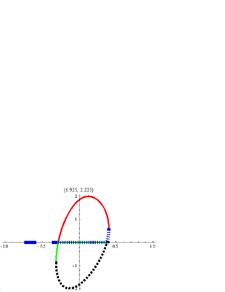
Figure 1: Left side of the expression (68) is plotted versus parameter $v=\lambda_{l,13}$ for the fixed values of $x=6.925,y=2.225$ and different signs before square roots in expressions for $\lambda_{l,23},$ see (69), and $\lambda_{l,12},$ see (70). We can see, that we can often satisfy (68) by properly choosing signs in expressions (69) and (70).

The probabilities given by (64) satisfy the relation in (19) which in this case looks as:

$$(x^{2}+1)y^{2}p_{\beta_{l}\alpha_{12}}+(y^{2}+1)x^{2}p_{\beta_{l}\alpha_{13}}+(x^{2}+y^{2})p_{\beta_{l}\alpha_{23}}=\frac{2}{3}(x^{2}y^{2}+y^{2}+x^{2})$$ (65)

Putting (64) into (65), we get an equation for $\mu$:

$$2\mu^{2}+(x-y)\mu-1=0\Rightarrow\mu=\frac{(y-x)\pm\sqrt{(x-y)^{2}+8}}{4}$$ (66)

We are interested in the case then all absolute value of lambdas are less than one

$$|\lambda_{l,{ij}}|<1,\forall\;ij=12,13,23.$$ (67)

It is satisfied when $|\mu|<1$. So, for the case of $|x-y|<1$ , for both roots of (66) conditions $|\lambda_{l,{ij}}|<1$ are valid, if $x-y>1$, then (66) with the plus sign suits $|\lambda_{l,{ij}}|<1$, otherwise $y-x>1$, then (66) with the minus sign is valid.
Now we proceed in a general case, i.e. without ansatz $\lambda_{l,12}=\mu,\;\lambda_{l,13}=-\mu,\;\lambda_{l,23}=1-2\mu^{2}$. Conditions (58) and (59) equation (19), which is equivalent to Born’s rule, comes down to:

$$y\lambda_{l,12}+x\lambda_{l,13}+\lambda_{l,23}=0$$ (68)

We should combine it with the constraint, see (62) for $\lambda_{l,12},\lambda_{l,13},\lambda_{l,23}$ to have simultaneous solution

$$\lambda_{l,23}=\lambda_{l,12}\lambda_{l,13}\pm\sqrt{(1-\lambda_{l,12}^{2})(1-\lambda_{l,13}^{2})}$$ (69)

We have two equations for three variables, thus we can express the solution as a one-parametric family. Let us choose $v=\lambda_{l,13}$ as a parameter. Then

$$\lambda_{l,12}=\frac{-xv(y+v)\pm\sqrt{(v^{2}-1)(v^{2}x^{2}-y^{2}-1-2yv)}}{y^{2}+1+2yv},$$ (70)

and $\lambda_{l,23}$ can be obtained from equation (62). We have to make sure that $\lambda_{l,12},\lambda_{l,13},\lambda_{l,23}$ exist, are real and satisfy (67), given real and positive x and y. In this, more general, case

$$p^{b|a}_{\beta_{l}\alpha_{1}}=\frac{1}{3}+\frac{2\lambda_{l,12}}{3\left(x+\frac{1}{x}\right)},\;p^{b|a}_{\beta_{l}\alpha_{1}}=\frac{1}{3}+\frac{2\lambda_{l,13}}{3\left(y+\frac{1}{y}\right)},\;p^{b|a}_{\beta_{l}\alpha_{1}}=\frac{1}{3}+\frac{2\lambda_{l,23}}{3\left(\frac{x}{y}+\frac{y}{x}\right)},$$ (71)

Seeing that all values in the parentheses in (64) are greater than 2, each of the this probabilities non-negative and smaller than 2/3, if $\lambda_{l,12},\lambda_{l,13},\lambda_{l,23}$ are smaller than 1. The main problem is to describe possible rangers of parameters in (70) which give us $|\lambda_{l,ij}|\leq 1$, see figure 1–3. W e remark that $\lambda_{l,13}$ is a a parameter, $|v|\leq 1$.

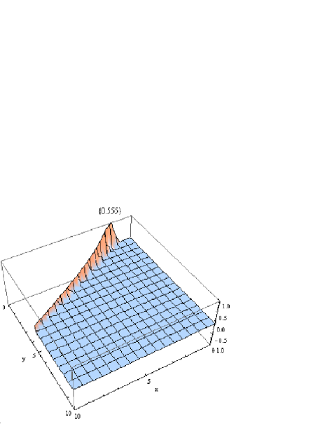
Figure 2: Left side of the expression (68) is plotted versus parameters $x,y,$ for the fixed $v=\lambda_{l,13}=0,555.$ Minus sign is taken before square root in (70), plus sign is taken in (69) when obtaining $\lambda_{l,13}$ values. We can see that it is equal to zero as (68) demands on a large scope of $x,y$ parameters values.

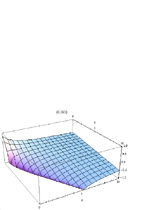
Figure 3: Value of $\lambda_{l,12}$ as function (70) of parameters $x,y,$ for the fixed $v=\lambda_{l,13}=0.585.$ Plus sign is taken before square root in 70). One may see that value $\lambda_{l,12}$ is within $(-1,1)$ limits for the most part of the values $x$ and $y.$

5.2 Complex amplitude matching Born’s rule for two observables

We now want to select an orthonormal basis $e_{\alpha}^{a}$ such that, for the state $\psi$ constructed in the previous section, $|\langle\psi|e_{\alpha}^{a}\rangle|^{2}=p_{\alpha}^{a}.$ We turn to considerations of section 2.5. Since vectors of this basis can be selected up to $e^{i\xi_{\alpha}}.$ We can select $\theta_{\beta_{1}\alpha_{k}}=\phi_{\beta_{1}\alpha_{k}},$ i.e., set $\xi_{\alpha}=0.$ Of course, to guarantee orthogonality of this basis, constraints (29), (30) should be taken into account:

$$\sum_{m}\sqrt{p_{\beta_{m}\alpha_{i}}p_{\beta_{m}\alpha_{j}}}\lambda_{m,ij}=0,$$ (72)

$$\sum_{m}\epsilon_{m,ij}\sqrt{p_{\beta_{m}\alpha_{i}}p_{\beta_{m}\alpha_{j}}}\sqrt{1-\lambda_{m,ij}^{2}}=0,$$ (73)

where $\epsilon_{m,ij}$ are signs which are selected in a proper way.

Moreover, the matrix of transition probabilities has to be doubly stochastic, i.e., besides (45), we should have

$$\sum_{l=j}^{3}p_{\beta_{l}\alpha_{j}}^{b|a}=1$$ (74)

for each $l=1,2,3.$

Under these conditions the complex amplitude $\psi$ produced by our algorithm matches with Born’s rule for both obsrevables, $a$ and $b.$

Example 1. We can take

$$\lambda_{1,12}=\mu,\;\lambda_{1,23}=-\mu,\lambda_{1,13}=0;$$

$$\lambda_{2,12}=-\mu,\lambda_{2,23}=0,\;\lambda_{2,13}=\mu;$$

$$\lambda_{3,12}=0,\;\lambda_{3,23}=\mu,\;\lambda_{3,13}=-\mu.$$

This gives us the solution $\mu=\frac{1}{\sqrt{2}}.$ First take the plus-case(e.i. $\mu=\pm\frac{1}{\sqrt{2}}$). We select $\phi_{m1}=\nu_{m},m=1,2,3.$ For $\beta_{1},$ we obtain the system of equations: $\cos(\nu_{1}-\phi_{12})=\frac{1}{\sqrt{2}},\cos(\phi_{12}-\phi_{13})=-\frac{1}{\sqrt{2}},\cos(\nu_{1}-\phi_{13})=0.$ Hence, $\phi_{11}=\nu_{1},$ and $\phi_{12}=\nu_{1}-\pi/4,\phi_{13}=\nu_{1}+\pi/2$ or $\phi_{12}=\nu_{1}+\pi/4,\phi_{13}=\nu_{1}-\pi/2.$

Then, for $\beta_{2},$ $\cos(\nu_{2}-\phi_{22})=-\frac{1}{\sqrt{2}},\cos(\phi_{22}-\phi_{23})=0,\cos(\nu_{2}-\phi_{23})=\frac{1}{\sqrt{2}}.$ Hence, $\phi_{21}=\nu_{2},$ and $\phi_{22}=\nu_{2}+3\pi/4,\phi_{23}=\nu_{2}+\pi/4$ or $\phi_{22}=\nu_{2}-3\pi/4,\phi_{23}=\nu_{2}-\pi/4.$ Finally, for $\beta_{3},$ $\cos(\nu_{3}-\phi_{32})=0,\cos(\phi_{32}-\phi_{33})=\frac{1}{\sqrt{2}},\cos(\nu_{3}-\phi_{33})=-\frac{1}{\sqrt{2}}.$ Hence, $\phi_{31}=\nu_{3},$ and $\phi_{32}=\nu_{3}+\pi/2,\phi_{33}=\nu_{3}+3\pi/4$ or $\phi_{32}=\nu_{3}-\pi/2,\phi_{33}=\nu_{3}-3\pi/4.$ We have from equation (7),(8) and (10) that

$$\psi_{\beta_{1}}=\sum_{i}\sqrt{p_{\alpha_{m}}^{a}p_{\beta_{l}\alpha_{m}}}e^{i(\xi_{\alpha_{i}}+\theta_{\beta_{l}\alpha_{m}})},$$

where $\xi_{\alpha_{i}}=0$ and $\sqrt{p_{\alpha_{m}}^{a}p_{\beta_{l}\alpha_{m}}}=\frac{1}{3}.$ Thus

$$\psi_{\beta_{1}}=\frac{1}{3}(e^{i\nu_{1}}+e^{i\nu_{1}\mp\pi/4}+e^{i\nu_{1}\pm\pi/2})=\frac{e^{i\nu_{1}}}{3}(1+e^{\mp i\pi/4}+e^{\pm i\pi/2})=\frac{e^{i\nu_{1}}}{3}((1+\frac{\sqrt{2}}{2})\pm i(1-\frac{\sqrt{2}}{2}));$$

$\psi_{\beta_{2}}=\frac{e^{i\nu_{2}}}{3}(1\pm i\sqrt{2})$ and, finally, $\psi_{\beta_{3}}=\frac{e^{i\nu_{3}}}{3}((1-\frac{1}{\sqrt{2}})\pm i(1+\frac{1}{\sqrt{2}})).$ We remark that $|\psi_{\beta_{j}}|^{2}=1/3,j=1,2,3.$

QLRA produces following possible realizations of the “wave function”:

$$\psi=\frac{1}{3}[((1+\frac{1}{\sqrt{2}})\pm i(1-\frac{1}{\sqrt{2}}))e_{\beta_{1}}^{b*}+(1\pm i\sqrt{2})e_{\beta_{2}}^{b}+((1-\frac{1}{\sqrt{2}})\pm i(1+\frac{1}{\sqrt{2}}))e_{\beta_{3}}^{b*}],$$ (75)

where $e_{\beta}^{b}$ are the orthonormal basis

$$e^{b}_{\beta_{1}}=\left(\begin{array}[]{ll}e^{i\nu_{1}}\\ 0\\ 0\end{array}\right),\;e^{b}_{\beta_{2}}=\left(\begin{array}[]{ll}0\\ e^{i\nu_{2}}\\ 0\end{array}\right),\;e^{b}_{\beta_{3}}=\left(\begin{array}[]{ll}0\\ 0\\ e^{i\nu_{3}}\end{array}\right).$$ (76)

For the minus-case (e.i. $\mu=-\frac{1}{\sqrt{2}}$) QLRA produces following “wave function”:

$$\psi=\frac{1}{3}[((1-\frac{1}{\sqrt{2}})\pm i(1+\frac{1}{\sqrt{2}}))e_{\beta_{1}}^{b}+(1\pm i\sqrt{2})e_{\beta_{2}}^{b}+((1+\frac{1}{\sqrt{2}})\pm i(1-\frac{1}{\sqrt{2}}))e_{\beta_{3}}^{b}].$$ (77)

Acknowledgments

One of the authors, Irina Basieva, is supported by Swedish Institute, post–doc fellowship. We would like to thank professor Andrei Khrennikov for fruitful discussions about quantum formalism and probability theory.

References

- [1] Neumann J. von, Mathematical foundations of quantum mechanics, Princeton Univ. Press, Princeton, N.J., 1955.
- [2] Gudder, S. P., Special methods for a generalized probability theory. Trans. AMS 119, 428 (1965).
- [3] Gudder, S. P., Axiomatic quantum mechanics and generalized probability theory, Academic Press, New York, 1970.
- [4] Gudder, S. P., An approach to quantum probability, Quantum Prob. White Noise Anal. 13, (147) (2001).
- [5] Ballentine, L. E., Interpretations of probability and quantum theory, Q. Prob. White Noise Anal. 13, 71 (2001).
- [6] Dvurecenskij A. and Pulmanova, O., New trends in quantum structures. Kluwer Academic Publ., Dordrecht, 2000.
- [7] Nánásiová, O., Map for simultaneous measurements for a quantum logic. International Journal of Theoretical Physics, 42 (2003), pp. 1889–1903.
- [8] Nánásiová, O. and Khrennikov, A. Yu., Representation theorem of observables on a quantum system. International Journal of Theoretical Physics 45 (2006), pp. 469–482.
- [9] A. Khrennikov, On the representation of contextual probabilistic dynamics in the complex Hilbert space: linear and nonlinear evolutions, Schrödinger dynamics, Il Nuovo Cimento, 120, N. 4, 353-366 (2005).
- [10] A. Khrennikov, A pre-quantum classical statistical model with infinite-dimensional phase space. J. Phys. A: Math. Gen., 38, 9051-9073 (2005).
- [11] A. Khrennikov, The Einstein-Podolsky-Rosen paradox and the -adic probability theory. Dokl. Mathematics, 54, N. 2, 790-795.
- [12] A. Khrennikov, Ja. I. Volovich, Discrete time dynamical models and their quantum-like context-dependent properties. J. Modern Optics, 51, N. 6/7, 113-114 (2004).
- [13] A. Khrennikov, Representation of probabilistic data by quantum-like hyperbolic amplitudes. Advances in Applied Clifford Algebras, 20 (1), 43-56 (2010).
- [14] Allahverdyan, A., Khrennikov, A. Yu. and Nieuwenhuizen, Th. M., Brownian entanglement, Phys. Rev. A, 71, (2005),032102-1 –032102-14.
- [15] Khrennikov, A. Yu., Interpretations of Probability. VSP International Science Publishers, Utrecht 1999; second addition (completed) De Gruyter, Berlin 2009.
- [16] Sinha, U. and Couteau, C. and Medendorp, Z. and Sollner, I. and Laflamme, R. and Sorkin, R. and Weihs, G., Testing Born’s Rule in Quantum Mechanics with a Triple Slit Experiment, Foundations of Probability and Physics- 5, 1101, 2009, pp. 200–207
- [17] Khrennikov, A. Yu., Contextual approach to quantum formalism. Fundamental theories of Physics 160, Springer Verlag, New York 2009
- [18] Khrennikov, A. Yu.,Quantum-like model of cognitive decision making and information processing, Biosystems, 95, 3, pp. 179–187, 2009, Elsevier
- [19] Nyman, P., On Consistency of the Quantum-Like Representation Algorithm, International Journal of Theoretical Physics, 49, 1, pp. 1–9, 2010, Springer
- [20] Nyman, P., On Consistency of the Quantum-Like Representation Algorithm for Hyperbolic Interference, Arxiv preprint quant-ph/1009.1744, 2010
- [21] Khrennikov, A. Yu., Reconstruction of quantum theory on the basis of the formula of total probability, Arxiv preprint quant-ph/0302194, 2003
- [22] Sorkin, R. D., Quantum Mechanics as Quantum Measure Theory, Modern Physics Letters A 9, pp. 3119–3127 (1994), arXiv:gr-qc/9401003.
- [23] Sorkin, R.D., Quantum Measure Theory and its Interpretation, in D.H. Feng and B-L Hu (eds.), Quantum Classical Correspondence: Proceedings of the 4th Drexel Symposium on Quantum Nonintegrability, International Press, Cambridge, pp. 229–251, 1997, arXiv:gr-qc/9507057v2